Robot Variable Impedance Control and Generalizing from Human–Robot Interaction Demonstrations

Abstract

The purpose of this study was to ensure the compliance and safety of a robot’s movements during interactions with the external environment. This paper proposes a control strategy for learning variable impedance characteristics from multiple sets of demonstration trajectories. This strategy can adapt to the control of different joints by adjusting the parameters of the variable impedance control policy. Firstly, multiple sets of demonstration trajectories are aligned on the time axis using Dynamic Time Warping. Subsequently, the variance obtained through Gaussian Mixture Regression and a variable impedance strategy based on an improved Softplus function are employed to represent the variance as the variable impedance characteristic of the robotic arm, thereby enabling variable impedance control for the robotic arm. The experiments conducted on a self-designed robotic arm demonstrate that, compared to other variable impedance methods, the motion accuracy of the trajectories of joints 1 to 4 improved by 57.23%, 3.66%, 5.36%, and 20.16%, respectively. Additionally, a stiffness-variable segmented generalization method based on Dynamic Movement Primitive is proposed to achieve variable impedance control in various task environments. This strategy fulfills the requirements for compliance and safety during robot interactions.

1. Introduction

An increasing number of robots of various forms have entered people’s daily lives, and people’s demands for their compliance, safety, and adaptability are constantly growing. Traditional position control can no longer meet people’s needs, leading to the increasingly widespread application of impedance control in human–robot interactions [1]. Learning from Demonstration (LfD) is a simple, efficient, and easy-to-master method for trajectory planning in position control [2]. However, it poses a challenge to learn variable impedance characteristics from demonstrated trajectories and transfer variable impedance control to different task trajectories and loading conditions in robot learning.

Variable impedance control adjusts impedance parameters dynamically based on the task requirements and environmental conditions to modify operational compliance and ensure a safe interaction and accurate task completion [3]. Estimating the variable impedance parameters from human demonstrations is a more effective approach. Yu [4] utilized the MYO device to collect electromyography (EMG) signals from the upper limb of the teacher to estimate its stiffness characteristics. Simultaneously, the joint motion trajectories of the JACO2 robotic arm were recorded. Dynamic Movement Primitive (DMP) was then employed to generalize and propagate the joint motion trajectories and variable stiffness profiles. Finally, the effectiveness of the trajectory generalization and stiffness profile generalization was validated through a pumping experiment using the JACO2 robotic arm. This approach not only enhanced safety but also improved the interactive capabilities of the robotic arm with its environment. Saveriano [5] performed Gaussian Mixture Regression (GMR) on the demonstrated trajectories and estimated the variable stiffness. By comparing it with a constant high stiffness, it was found that variable stiffness impedance control better demonstrates smoothness and safety during an interaction with the external environment. Zhang [6] utilized GMR to estimate the variable stiffness profiles for translation and rotation by analyzing the demonstrated trajectories. To validate the adaptability of variable stiffness impedance control to environmental changes, they conducted a pouring experiment using bottles of different weights and shapes. The experiment confirmed the effectiveness of variable stiffness impedance control in adapting to variations in the interaction environment. Liao [7] employed an extended DMP framework for learning and generalizing in three aspects: position, orientation, and stiffness. This successful implementation enabled the robot to achieve human-like variable impedance control, enhancing the applicability of the robotic arm in interactive processes and enabling the robotic arm to possess learning capabilities. Yang [8] employed the MYO device to monitor the real-time muscle activity of the teacher’s upper limb. The estimated endpoint stiffness was then mapped to the impedance controller of the robotic arm. Variable impedance control was achieved in the context of cutting experiments and lifting tasks using the dual-arm Baxter robot. The motion trajectories and variable stiffness profiles were generalized and extended using the DMP framework, enabling adaptability to a wider range of interactive environments. Wu [9] also utilized the MYO device to collect surface EMG signals from the human forearm. By combining these signals with the forearm posture, a real-time estimation of the arm’s stiffness gain was achieved. The estimated stiffness gain was then transmitted in real time to the KUKA LBR IIWA 14 R820 robotic arm. Calinon [10] encoded and reproduced the motion trajectories of the robotic arm using Gaussian Mixture Model (GMM) and GMR. In the GMR process, the covariance was considered to be the variability in an unstructured environment. The inverse of this covariance was then used as the variable stiffness in impedance control. The feasibility of the method was validated through experiments using the Barrett WAM robotic arm. Wu [11] also encoded and reproduced the motion trajectories of the robotic arm using GMM and GMR. Then, a linear quadratic regulator was employed to express the robot’s full Cartesian impedance, and the optimal impedance was achieved through a Cartesian impedance controller on the Franka Emika Panda robot. Mathew [12] employed a time-independent forward model to predict measurement errors. The forward model was continuously updated, and the impedance parameters of the feedback controller were modified accordingly. The approach allowed for accurate error prediction and enabled real-time adjustments to the impedance parameters of the feedback controller. However, the acquisition of variable impedance control skills using muscle EMG sensors is characterized by complexity and low efficiency, and strategies based on other sensors lack the ability to adjust variable impedance control strategies, making it challenging to meet the requirements of different structure robots or parameter adjustments. Therefore, this paper proposes a method to learn variable impedance skills from demonstrated trajectories. The authors designed indicator functions based on the Softplus function as the basis function for variable stiffness and variable damping. These indicator functions can be adjusted by modifying their parameters, allowing for adaptability to variable impedance control for different types of robots. Thus, the variable impedance characteristics of the human arm are converted into the variable impedance characteristics of the robotic arm. The advantage of this method lies in its ability to learn, replicate, and optimize the interactive behavior of the robotic arm, enabling it to handle various operational tasks.

The main contributions of this study are as follows:

• To achieve the transfer of variable impedance skills from the human to the robotic arm, a variable impedance control strategy is proposed to learn impedance characteristics from multiple sets of demonstration trajectories. Firstly, the demonstration trajectories are aligned on the time axis through Dynamic Time Warping (DTW). Then, using the variance obtained from GMR, the control strategy represents the variance as impedance control parameters based on an improved Softplus function, enabling variable impedance control of the robotic arm.
• To adapt variable impedance control to different task environments, a segmented generalized approach for variable stiffness based on DMP is proposed. This method utilizes stationary points with monotonicity in the variable stiffness profile as segmentation points and performs segmented generalization to satisfy the requirements of variable impedance control.

Overall, the combination of LfD, GMR, variable impedance indicator functions, DMP, and variable stiffness transfer in this framework enhances the accuracy and adaptability of impedance control in robotic systems.

The remaining sections of this paper are organized as follows. Section 2 provides the variable stiffness control strategy and the DMP framework. In Section 3, experiments are conducted to validate the feasibility, safety, and accuracy of variable stiffness transfer through trajectory generalization and variations in the end-effector load. Finally, Section 4 summarizes the findings and concludes this article.

2. Materials and Methods

Transferring human skills to robots to enable accurate and safe task completion in unknown environments is a reasonable approach [13,14]. In the context of a laboratory setting, the process starts by collecting multi-demonstration trajectories using a Kinect sensor. Since the duration of each demonstration trajectory is difficult to maintain consistently, DTW is used to align the trajectories on the time axis. Finally, GMM and GMR are employed to regress the multi-demonstration trajectories into a single better motion trajectory. Additionally, GMR is utilized to calculate the standard deviation of the motion trajectory during the regression process, which is then used to estimate the impedance profile. However, the regression trajectory obtained through GMR only ensures the contour of the robot’s motion trajectory and does not guarantee the precision of the initial and final positions of the robot’s motion. Therefore, DMP can be employed to generalize the robot’s motion trajectory, ensuring both the trajectory’s contour and its precision.

In conjunction with a self-designed robotic arm, a variable impedance control strategy is devised to ensure a safe interaction and accurate task completion in a human–robot coexistence environment. This strategy guarantees the control precision of the robotic arm during impedance control. Additionally, a framework based on DMP is proposed, enabling the learning and generalization of variable impedance manipulation skills from human demonstrations. By learning the variable impedance control strategy, the robotic assistant can intelligently adjust its compliance to adapt to environmental changes. Whether the load connected to the robotic arm’s end effector changes or the joint motion trajectory of the robotic arm varies, the variable impedance strategy based on DMP can be transferred to meet the requirements of different tasks. In Figure 1, the entire process of the variable impedance control strategy is illustrated.

2.1. Variable Impedance Control Strategy

The variable stiffness profile can be effectively estimated from the demonstration trajectories [10]. By using GMM–GMR to regress multi-demonstration trajectories, reasonable variable impedance skills are learned from the variance of the regression trajectories, mapping the variance of the demonstration trajectories to the stiffness profile to adapt to the changing task environment of the robotic arm. By learning the demonstration trajectory of the human arm, the variable impedance characteristics of the human arm are converted to the variable impedance characteristics of the robotic arm. The basic idea is that in the part where the variance of the demonstration trajectory is small, the robotic arm joint should maintain a high stiffness level to ensure accurate tracking of the reference trajectory [6]. For the part with large variance, the robotic arm joint can be kept at a relatively low stiffness level to ensure the flexibility of operation, and the Softplus function can meet this characteristic. Therefore, in order to meet the variable stiffness profile of the adaptive task, an indicator function of variable stiffness and variable damping based on the Softplus function is proposed, as shown in Equations (1)–(3).

$${\chi }_l(t)=(1-a_l)({\chi }_l^{\max }-{\chi }_l^{\min })+{\displaystyle \frac{{\chi }_l^{\max }+{\chi }_l^{\min }}{c{c}_l}}$$

(1)

$$a_l=\ln (1+e^{bl})$$

(2)

$$b_l={\displaystyle \frac{c_l\sqrt{d_l}-d_l^{\min }}{d_l^{\max }-d_l^{\min }}}$$

(3)

where ${\chi }_l^{\max }$ and ${\chi }_l^{\min }$ represent the maximum and minimum stiffness/damping values in the l direction, and $d_l^{\max }$ and $d_l^{\min }$ represent the maximum and minimum standard deviations in the l direction. l denotes each joint of the robotic arm. The values of c and cc can be flexibly adjusted according to the requirements of the variable stiffness and variable damping profiles. Therefore, this indicator function is not only applicable for stiffness profiles but also suitable for damping profiles.

To calculate the driving torque Γ based on Equation (4) of the variable impedance control equation, given the variable stiffness K_p and variable damping K_d:

$$\mathrm{\Gamma }=K_p(q_d-q)+K_d(q_d^{\prime }-q^{\prime })+{\mathrm{\Gamma }}_{ff}$$

(4)

where the stiffness matrix K_p = diag (K_p), the damping matrix K_d = diag (K_d), and Γ_ff represents the feed forward term of the joint torque, which is calculated based on identified dynamic parameters [15] (dynamics literature [15] published by the author). q_d and q denote the desired and actual joint positions, respectively. q_d′ and q_d denote the desired and actual joint velocities, respectively. The impedance controller of the second order is used to calculate the torque of each joint, and then the calculated value of the joint torque is sent to the corresponding robotic arm joint so as to drive the motion of the robotic arm joint.

2.2. Stability Analysis of the Robot

Impedance control is a typical second-order PD controller. When the end point of the robotic arm is controlled at a fixed point, the desired position q_d is reached.

The general formula of robotic arm dynamics is

$$\mathrm{\Gamma }=M(q)q^{″}+C(q,q^{\prime })q^{\prime }+G(q)$$

(5)

The following can be obtained from Equation (4):

$$\mathrm{\Gamma }-{\mathrm{\Gamma }}_{ff}=K_p(q_d-q)+K_d(q_d^{\prime }-q^{\prime })$$

(6)

According to Equations (5) and (6), the following can be obtained:

$$M(q)(q_d^{″}-q^{″})+C(q,q^{\prime })q^{\prime }=K_p(q_d-q)+K_d(q_d^{\prime }-q^{\prime })$$

(7)

Let q_d − q = e; then, Equation (7) is converted to

$$M(q)e^{″}+C(q,q^{\prime })e^{\prime }+K_{p}e+K_d{e}^{\prime }=0$$

(8)

The Lyapunov function V(q) under this controller (8) is given as

$$V(q)={\displaystyle \frac{1}{2}}{e^{\prime }}^{T}M(q)e^{\prime }+{\displaystyle \frac{1}{2}}{e}^T{K}_{p}e$$

(9)

Since M(q) and K_p are both positive definite matrices, V(q) can be obtained as a global positive definite, and the derivation of it can be obtained as follows:

$$V^{\prime }(q)=e^{\prime T}M(q)e^{″}+{\displaystyle \frac{1}{2}}{e}^{\prime T}{M}^{\prime }(q)e^{\prime }+{e^{\prime }}^T{K}_{p}e$$

(10)

Using the anti-symmetry of $M^{\prime }(q)-2C(q,q^{\prime })$ to know $e^{\prime T}{M}^{\prime }(q)e^{\prime }=2e^{\prime T}C(q,q^{\prime })e^{\prime }$, the following is obtained:

$$\begin{array}{l}{V}^{\prime }(q)=e^{\prime T}M(q)e^{″}+e^{\prime T}C(q,q^{\prime })e^{\prime }+e^{\prime T}{K}_{p}e\\ =e^{\prime T}(M(q)e^{″}+C(q,q^{\prime })e^{\prime }+K_{p}e)\\ =-e^{\prime T}{K}_{p}e\le 0\end{array}$$

(11)

From the positive qualitative of K_d, we can know $V^{\prime }(q)\le 0$; then, $V^{\prime }(q)$ is a semi-negative qualitative. Therefore, according to Lyapunov’s second method, it can be proved that the system is globally asymptotically stable.

2.3. DMP for Generalization and Transfer

To enhance the adaptability of a robotic arm to changes in the external environment, DMPs are extended with a variable stiffness transfer component. After obtaining the desired motion trajectory through GMR, the regression trajectory is further generalized to accommodate different target tasks at various positions. This generalization is applied to both position and orientation trajectories [16] as well as stiffness trajectories [8,17,18]. For robotic motion in Cartesian or joint space, DMPs can be used to model trajectories by capturing the features of the input trajectories, including the initial and target values. This enables the rapid generation of new trajectories with the same learned trajectory features but different input initial and target values, facilitating motion generalization.

Essentially, DMPs represent a second-order system with spring-damper dynamics augmented by a forcing term. They have the capability to generalize trajectories to new starting and target positions [19]. The expression for DMPs is as follows:

$${\tau }^2\dot{v}=\alpha (\beta (g-x)-\tau v)+f(s)$$

(12)

where x and v represent the current position and velocity of the robot, respectively. g represents goal position. α and β represent the coefficients of the spring-damping system. τ is a positive constant temporal factor, and f(s) is the non-linear force term used to generate expected movements.

For the Canonical System,

$$\tau \dot{s}=-{\alpha }_{s}s$$

(13)

where α_ss is a predefined constant. s∈(0, 1] is set to monotonically decrease from 1 to 0. The initial value is set to s(0) = 1. The forcing term f(s) is expressed using basis functions as follows:

$$f(s)={\displaystyle \frac{{\displaystyle {\sum }_{i=1}^N{\omega }_i{\psi }_i(s)}}{{\displaystyle {\sum }_{i=1}^N{\psi }_i(s)}}}s(g-x_0)$$

(14)

$${\psi }_i(s)=\exp (-{\displaystyle \frac{1}{2{\sigma }_i^2}}{(s-c_i)}^2)$$

(15)

where ψ_i(s) is the Gaussian basis function, ω_i is weighted, c_i represents the center of the function, and σ_i represents the variance of the function. N represents the total number of basic functions, and x₀ represents the initial position.

3. Results and Discussion

This experimental study utilized a self-designed robotic arm, as shown in Figure 2. Due to the symmetry of both arms, the right arm is now the research object. An impedance control method was employed to achieve joint adjustments. The Kinect sensor was used to capture the joint trajectories of the teacher. The stiffness variation indicator was calculated from the standard deviation of the multi-demonstration trajectories regression process. Based on the previous introduction, the impedance control framework with variable impedance based on the demonstration trajectory could be divided into two main parts: learning reasonable variable impedance operational skills from the demonstration trajectory and enabling the robot to generalize the reference stiffness profile to adapt to changes in the task environment of the robotic arm.

3.1. Demonstration Trajectory Based on Kinect Acquisition

According to the author’s published literature [20], the structure of the self-designed robot was analyzed in the literature, the inverse kinematics of the self-designed robotic arm was solved using the D-H method and screw theory, and the demonstration trajectory of each joint of the robotic arm was collected in real time by a Kinect sensor to complete the collection of the demonstration trajectory. It is known that the end effector Cartesian space trajectory of the self-designed robotic arm is obtained through the first four joints of the robotic arm. However, the performance of the Kinect sensor in data acquisition is not stable, resulting in a relatively inaccurate calculation of the robotic arm’s posture. Therefore, in this paper, the focus was mainly on impedance control based on the end effector trajectory of the robotic arm, specifically the solution and control of joints 1, 2, 3, and 4 of the robotic arm. In this paper, 10 groups of demonstration joint trajectories of the right arm were collected. Multiple joint demonstration trajectories were aligned in a time series using DTW [21,22], as shown in Figure 3. From the figure, it can be observed that the multiple joint demonstration trajectories, after being processed by DTW, were not only aligned in the time series but also retained the characteristics of the original demonstration trajectories. The overall effect of the processing satisfied the requirements for subsequent GMR.

Finally, GMM–GMR was utilized to perform a regression on the position data of each joint [23,24]. The number of Gaussian distributions for each joint position data was set to 2, 2, 3, 3, as shown in Figure 4.

The estimated variable stiffness profile and variable damping profile were obtained based on the regression of the multi-demonstration trajectories, and the standard deviation of the regression trajectories is shown in Figure 5.

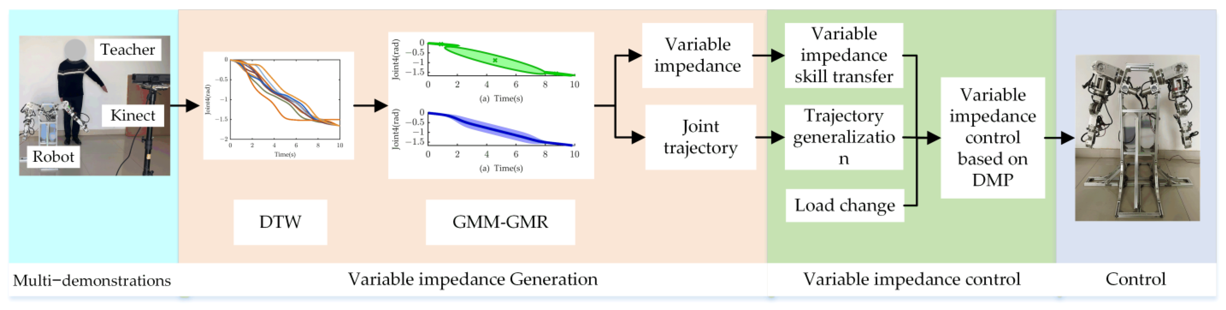
3.2. Validation of the Variable Impedance Control Strategy for the Robotic Arm

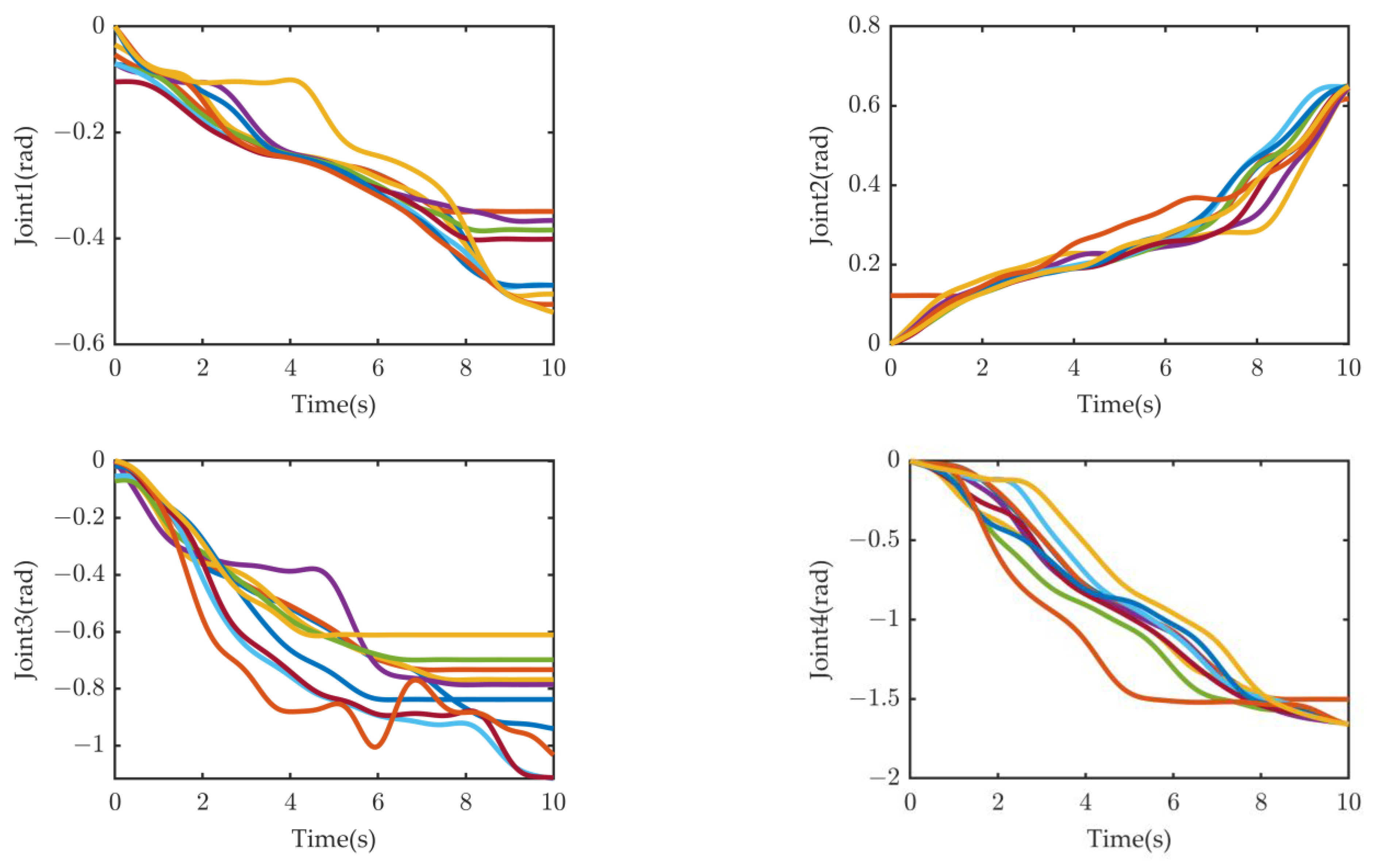
The regression trajectories obtained by processing multiple sets of demonstration trajectories through DTW–GMM–GMR were input into the DMP model for learning to improve the accuracy of reproducing the demonstration trajectories. According to the different task trajectories, by changing the initial and target positions of the joint motion trajectory, a generalized trajectory with the same motion trend as the demonstration trajectory can be obtained, which can meet the requirements of different task initial and target positions. The initial and target positions of the regression trajectory are shown in

Table 1. Position of the regression trajectory (units: rad).

Parameters	Joint 1	Joint 2	Joint 3	Joint 4
Initial Position	−0.0556	0.0495	−0.0066	−0.0079
Target Position	−0.4942	0.6266	−0.8634	−1.6833

. According to the task requirements, the regression demonstration trajectory was generalized, and the generalized trajectory is called trajectory 1. The initial and target positions of trajectory 1 were set as shown in

Table 2. DMP model generalized trajectory 1 (units: rad).

Parameters	Joint 1	Joint 2	Joint 3	Joint 4
Setting the Initial Position	0	0	0	0
Setting the Target Position	−0.5236	0.6981	−0.9599	−1.3963
Generalize the Initial Position	−4.5066 × 10−4	3.2555 × 10−4	−1.6655 × 10−3	−4.1159 × 10−4
Generalize the Target Position	−0.5235	0.6979	−0.9598	−1.3965

. Setting the parameters α to 35 and β to 35/4 = 8.75, the initial and target positions of the motion trajectory after generalization by the DMP model are shown in Table 2. According to the analysis in Table 2, the error between the initial position and the set initial position of trajectory 1 after generalization, as well as the error between the target position and the set target position, can meet the task requirements of trajectory design, as shown in

Table 3. Position error of DMP model generalized trajectory 1 (units: rad).

Parameters	Joint 1	Joint 2	Joint 3	Joint 4
Initial Position Error	−4.5066 × 10−4	3.2555 × 10−4	−1.6655 × 10−3	−4.1159 × 10−4
Target Position Error	−1.0 × 10−4	−2.0 × 10−4	1.0 × 10−4	−2.0 × 10−4

. As shown in Figure 6, the generalized trajectory 1 demonstrates the accuracy of the trajectory generalization of the DMP model.

In the motion experiment of the robotic arm without a load, the maximum stiffness k_max and minimum stiffness value k_min for joints 1 to 4 are shown in

Table 4. Joints 1 to 4 maximum and minimum allowable stiffness values (units: N·m/rad).

Parameters	Joint 1	Joint 2	Joint 3	Joint 4
kmax	225.88	272.57	217.85	126.36
kmin	54.21	144.3	150.82	87.48

. The maximum damping d_max and minimum damping d_min for joints 1 to 4 are shown in

Table 5. Joints 1 to 4 maximum and minimum allowable damping values (units: N·m·s/rad).

Parameters	Joint 1	Joint 2	Joint 3	Joint 4
dmax	408.59	62.57	8.85	25.52
dmin	96.77	33.13	4.43	17.67

. According to the task characteristics of each joint and the indicative functions in Equations (1) and (2), the values of the variable stiffness c₁ adjustment process for joints 1 to 4, the variable damping cc₂ adjustment process, and the variable damping cc₃ adjustment process are shown in

Table 6. Variable impedance control coefficient.

Parameters	Joint 1	Joint 2	Joint 3	Joint 4
c1	2.1	2.0	1.3	2.0
cc2	2.1	2.2	2.2	2.2
cc3	0.035	0.012	0.140	0.145

. Based on the parameters shown in Table 4, Table 5 and Table 6, the variable stiffness profile and variable damping profile were obtained, as shown in Figure 7 and Figure 8.

To validate the superiority of the proposed variable impedance control strategy in this paper, a comparison was made with the method presented in reference [6]. When running the variable impedance control strategy from reference [6], all parameters were set exactly the same as those in the proposed variable impedance control strategy in this paper. Equation (4) was used to calculate the torque required for the generalized trajectory to execute in torque mode and send the torque to the corresponding joint without any load or impact. During the torque application process, the joint angles of the robotic arm were recorded for two cases, as shown in Figure 9. The angle errors for joints 1 to 4 in two cases are illustrated in Figure 10. Finally, the Residual Standard Deviation (RSD) of the joint angles was used to evaluate the superiority, as shown in

Table 7. RSD of joint angles.

Method	Joint 1	Joint 2	Joint 3	Joint 4
Paper	0.0355	0.0184	0.0053	0.0099
Reference [6]	0.0830	0.0191	0.0056	0.0124

.

$${\epsilon }_{RSD}=\sqrt{{\displaystyle \frac{{\displaystyle \sum _{k=1}^K{({\sigma }_k-{\sigma }_k^{\prime })}^2}}{{\displaystyle \sum _{k=1}^K{\sigma }_k^2}}}}$$

(16)

where K represents the number of samples, σ_k represents the desired joint angles, and ${\sigma }_k^{\prime }$ represents the joint angles generated by the proposed variable impedance control strategy in this paper, or the joint angles generated by the variable impedance control strategy proposed in the reference literature.

By analyzing Figure 9, it can be observed that the proposed variable stiffness and variable damping control strategies in this paper make the motion of the robotic arm more stable, without significant fluctuations.

Based on the RSD values of the joint trajectories and the analysis of Figure 11 and Table 7, it can be seen that the variable impedance control strategy proposed in this paper has significantly improved the accuracy of joint 1′s motion trajectory, and joint 2 to joint 4 have also been improved to varying degrees. The trajectory accuracy of joint 1 to joint 4 has been improved by 57.23%, 3.66%, 5.36%, and 20.16%. Therefore, the variable impedance control strategy proposed in this paper has significantly improved the motion accuracy of the robotic arm.

To verify the safety and flexibility of the proposed variable stiffness and variable impedance strategies, a large random impact force was applied to the robotic arm at the 3rd second. The angles of the robotic arm’s joints were recorded during the experimental process, as shown in Figure 12.

From Figure 12, it can be observed that the angle errors of each joint of the robotic arm at the last moment under external impact are −0.008 rad, −0.0007 rad, −0.0001 rad, and 0.0042 rad. The robotic arm was able to recover to the desired values within a certain period of time, demonstrating its compliance and safety in interacting with the external environment.

3.3. Transfer Experiment of Robotic Arm’s Variable Impedance Control

To validate that DMPs have not only the ability to generalize robotic arm joint trajectories but also the ability to transfer and generalize variable stiffness skills, ensuring smooth control in different tasks, the generalization capability of DMP was extended from position control mode to impedance control mode. In this experiment, the generalized trajectory from Section 3.2, referred to as trajectory 1, as shown in Figure 6, was used. Then, a different trajectory was generated using DMP, referred to as trajectory 2, which was distinct from trajectory 1. The robotic arm followed this newly generalized trajectory for its motion. To assess the impact of changes in the task trajectory and an increase in load on the transfer and the generalization of variable stiffness skills, five tasks were designed as follows. In Figure 13, the specific task planning process is illustrated.

Task 1: The robotic arm follows the motion trajectory from Section 3.2, referred to as trajectory 1, and the variable stiffness profile is learned from the regression trajectory.

Task 2: The robotic arm follows trajectory 2 as the desired motion trajectory and utilizes the variable stiffness and variable damping obtained from Task 1 for impedance control.

Task 3: The robotic arm follows trajectory 2 as the desired motion trajectory and utilizes DMP to transfer and generalize the variable stiffness profile learned from Task 1 for impedance control.

Task 4: The robotic arm follows trajectory 2 as the desired motion trajectory while carrying a payload with dimensions of 200 mm × 110 mm × 100 mm and a weight of 2.66 kg. It utilizes the impedance control with variable stiffness and variable damping obtained from Task 3 to perform impedance control in this situation.

Task 5: The robotic arm follows trajectory 2 as the desired motion trajectory and utilizes DMP to transfer and generalize the variable stiffness profile learned from Task 3 for impedance control.

As a reference, if the actual trajectory followed by the robotic arm is the same as or very close to the desired trajectory, the task is considered successful. The specific process and result analysis for each task is presented below.

• Task 1: Feasibility study of variable stiffness

The specific process and result analysis are presented as described in Section 3.2.

• Task 2: Regeneralization based on the regression trajectory, which is different from the Task 1 environment

Based on the regression trajectory, the generalization is performed again, which is different from the generalization trajectory 1 in Section 3.2, making it easier to distinguish the generalization trajectory in Section 3.2. The generalization trajectory in this section is trajectory 2, and the initial and target positions of the joint trajectory for trajectory 2 are set as shown in

Table 8. Position of trajectory 2 (units: N·m/rad).

Parameters	Joint 1	Joint 2	Joint 3	Joint 4
Setting the Initial Position	−0.0556	0.0495	−0.0066	−0.0079
Setting the Target Position	−0.6981	0.8727	−1.1344	−1.5708
Generalize the Initial Position	−6.0088 × 10−4	4.0693 × 1000−4	−1.9684 × 10−3	−4.6303 × 10−4
Generalize the Target Position	−0.6980	0.8723	−1.1344	−1.5711

. We set the parameters α to 35 and β to 35/4 = 8.75. After generalization by the DMP model, the initial and target positions of trajectory 2 are shown in Table 8. According to the analysis in Table 8, the error between the initial setting and the initial position of trajectory 2 after generalization, as well as the error between the target position and the set target position of trajectory 2 after generalization, could meet the task requirements of the trajectory design, as shown in

Table 9. Position error of DMP model generalized trajectory 2 (units: rad).

Parameters	Joint 1	Joint 2	Joint 3	Joint 4
Initial Position Error	−6.0088 × 10−4	4.0693 × 10−4	−1.9684 × 10−3	−4.6303 × 10−4
Target Position Error	1.0 × 10−4	−4.0 × 10−4	0	3.0 × 10−4

. As shown in Figure 14, the generalized trajectory 2 demonstrates the accuracy of the trajectory generalization of the DMP model.

According to the requirements of Task 2, the robotic arm followed trajectory 2 as the desired motion trajectory, while the stiffness and damping adopted the variable stiffness and variable damping profiles from trajectory 1. No load was applied to the end effector of the robotic arm. The changes in joint angles during the experiment are depicted in Figure 15.

Figure 15 represents the trajectory generated using impedance control with the variable stiffness and variable damping from Task 1, with trajectory 2 as the desired motion trajectory. Comparing the end points of this trajectory to the desired trajectory 2, the end point errors for joints 1 to 4 are 0.0196 rad, −0.0106 rad, −0.0060 rad, and 0.0019 rad. Additionally, the RSD values for joints 1 to 4 are 0.0259, 0.0149, 0.0055, and 0.0089. Joints 1 and 2 exhibit larger end point errors, while joints 3 and 4 have smaller errors. As a result, only the variable stiffness transfer was applied to joints 1 and 2.

• Task 3: Variable stiffness generalization based on the environment of Task 2

Through Task 2, it can be seen that the impedance parameters of Task 1 did not meet the requirements of impedance control in Task 2. Therefore, the variable stiffness values of Task 1 were generalized using the DMP model to meet the requirements of Task 2. However, during the generalization of the variable stiffness profile, when the target stiffness value exceeded the initial stiffness value, the generalized stiffness curve tended to be opposite to the original stiffness curve. For example, the actual first joint variable stiffness profile is shown in Figure 7, which is an increasing curve in the 0–4.35 s interval and a decreasing curve in the 4.35–10 s interval, as shown in Equation (17). Therefore, the stationary point of the variable stiffness profile was taken as the segment point, and each segment was kept monotonic to achieve the generalization of each segment and meet the requirements of variable impedance control. It is believed that the 87th sample of the first joint was the point of monotonic segmentation, t = 4.35 s. The segmentation points of the other joints were also determined in the same way. When the whole variable stiffness profile of the first joint was generalized, its variable stiffness profile is shown in Figure 16, which is a decreasing curve in the 0–4.35 s interval and an increasing curve in the 4.35–10 s interval, opposite to the original trend of the variable stiffness profile, and it does not meet the requirements of generalization. Therefore, this chapter proposes to divide the variable stiffness profile of each joint into multiple monotonic trajectories using the DMP model, with the monotonic segmentation point as the segmentation point, and divide the variable stiffness profile into multiple monotonic trajectories. The segmentation point serves as the target value of the previous trajectory and the starting value of the subsequent trajectory. From the joint variable stiffness profile, it can be seen that the monotonic segmentation points of the first and second joints were 4.35 s and 7.05 s, respectively, as shown in Equations (18) and (19). Then, all joint stiffness profiles could be generalized based on the DMP model in a segmented manner, and the generalized variable stiffness profile is shown in Figure 17.

$$\begin{array}{l}{k}_1^{\prime }={\displaystyle \frac{k_1(k_n=87)-k_1(k_n=86)}{\mathsf{\Delta }t}}=0.77>0\\ k_1^{\prime }={\displaystyle \frac{k_1(k_n=88)-k_1(k_n=87)}{\mathsf{\Delta }t}}=-0.074<0\end{array}$$

(17)

$$\begin{array}{l}{\tilde{X}}_1=[{\tilde{x}}_1(t=0),{\tilde{x}}_1(t=4.35)]\\ {\tilde{G}}_1=[{\tilde{x}}_1(t=4.35),{\tilde{g}}_1]\end{array}$$

(18)

$$\begin{array}{l}{\tilde{X}}_2=[{\tilde{x}}_2(t=0),{\tilde{x}}_2(t=7.05)]\\ {\tilde{G}}_2=[{\tilde{x}}_2(t=7.05),{\tilde{g}}_2]\end{array}$$

(19)

After the segmented learning of variable stiffness for joint 1 and joint 2 based on the DMP model, it can be seen from Figure 18 that the joint end errors of joint 1 and joint 2 after variable stiffness generalization are 0.0012 rad and −0.0021 rad, respectively, and the joint error values are relatively small. In addition, the RSD values of joint 1 and joint 2 trajectories relative to the expected trajectory 2 are 0.0168 and 0.0140, respectively. Compared to task 2, according to the analysis of the RSD values in

Table 10. RSD values for Task 2 and Task 3.

Task	Joint 1	Joint 2
Task 2	0.0259	0.0149
Task 3	0.0168	0.0140

, it can be seen that the joint trajectory accuracy of joint 1 and joint 2 improved by 35.14% and 6.04%, respectively. From this, it can be seen that after the task trajectory changed, by performing variable stiffness generalization on the corresponding joints, it was possible to compensate for the changes in the required torque of the joints caused by the task changes, improve the accuracy of the joint motion trajectory, and meet the requirements of the task.

• Task 4: Change the load of the robotic arm based on the environment different from Task 3

The robotic arm followed trajectory 2 as the desired motion trajectory while carrying a payload with dimensions of 200 mm × 110 mm × 100 mm and a weight of 2.66 kg. It utilized the impedance control with variable stiffness and variable damping obtained from Task 3 to perform impedance control in this situation. The angle changes from joint 1 to 4 during the experiment are shown in Figure 19.

According to Figure 19, the end point errors for joints 1 to 4 of the robotic arm are 0.1066 rad, −0.0420 rad, −0.0207 rad, and 0.4791 rad. The RSD values for the trajectories of joints 1 to 4 are 0.1343, 0.0345, 0.0148, and 0.1569. Therefore, it can be observed that during the variable impedance control in Task 4, joint 1 gradually deviated from the desired trajectory starting from the 3rd second. Joint 4 also gradually deviated from the desired trajectory starting from the 2nd second and at the 8th second, there was a sudden and significant deviation from the desired trajectory for joint 4. Joints 2 and 3 also exhibited varying degrees of deviation from the desired trajectory. This deviation indicates that the task failed.

• Task 5: Variable stiffness generalization based on the load variation in Task 4

According to Task 4, the variable stiffness value of Task 3 did not meet the requirements of Task 4. Therefore, the variable stiffness value of Task 3 was then segmented based on the DMP model to meet the requirements of Task 4. However, in the process of variable stiffness value generalization, the third joint had the same situation as the first joint in the overall stiffness generalization, and the monotony of the contour curve was opposite, which could meet the requirements of variable stiffness generalization. Moreover, the segment trend of the third joint was more complicated. In addition, the variable stiffness profile trend of the third joint was more complex. According to the variable stiffness profile of the third section, it was divided into three sections, and the section points were 4.9 s and 7.2 s. In the process of global stiffness generalization, the fourth joint showed a negative stiffness value and a serious generalization error, as shown in Figure 20. According to the variable stiffness profile of the fourth joint, it was divided into two segments, with the segment point being 3.5 s. According to Task 3, piecewise DMP model learning was still carried out for the variable stiffness contour of each joint of the robotic arm. The piecewise point of the third and fourth joint is shown in Equations (20) and (21), and the variable stiffness contour of the third and fourth joint was generalized piecewise. The variation trend in the variable stiffness profile of the third joint and the fourth joint was satisfied, as shown in Figure 21.

$$\begin{array}{l}{\tilde{X}}_3=[{\tilde{x}}_3(t=0),{\tilde{x}}_3(t=4.9),{\tilde{x}}_3(t=7.2)]\\ {\tilde{G}}_3=[{\tilde{x}}_3(t=4.9),{\tilde{x}}_3(t=7.2),{\tilde{g}}_3]\end{array}$$

(20)

$$\begin{array}{l}{\tilde{X}}_4=[{\tilde{x}}_4(t=0),{\tilde{x}}_4(t=3.5)]\\ {\tilde{G}}_4=[{\tilde{x}}_4(t=3.5),{\tilde{g}}_4]\end{array}$$

(21)

After the generalization of the variable stiffness profile, this experiment showed that the joint trajectories of the robotic arm from joints 1 to 4, as shown in Figure 22, had end effector errors of 0.0081 rad, −0.0046 rad, −0.0097 rad, and 6.5347 × 10⁻⁵ rad. The end effector errors of each joint trajectory were relatively small, meeting the requirements of end effector accuracy. The RSD values of the trajectories from joint 1 to joint 4 relative to the expected Trajectory 2 are 0.0199, 0.0133, 0.0078, and 0.0211. Compared to Task 4, the RSD value analysis in

Table 11. RSD values for Task 4 and Task 5.

Task	Joint 1	Joint 2	Joint 3	Joint 4
Task 4	0.1343	0.0345	0.0148	0.1569
Task 5	0.0199	0.0133	0.0078	0.0211

shows that the joint motion trajectory accuracy of joints 1 to 4 increased by 85.18%, 61.45%, 47.30%, and 86.55%. From this, it can be seen that the motion trajectory generalized by variable stiffness met the requirements of Task 5. By adjusting the variable impedance parameter profile, the torque output by the motor met the motor torque requirements of the task.

To more clearly illustrate the differences between Task 4 and Task 5, the actual experimental process of the robotic arm’s variable impedance is shown in Figure 23. In the process of Task 4, the trajectory of motion began to deviate slightly at 2 s, and the fourth joint’s trajectory of motion deviated seriously downward at 8 s, which was not sufficient to lift the load. In addition, after returning to the initial position at 10 s, the robotic arm still maintained a deformed posture, that is, the robotic arm did not completely point straight down. On the other hand, Task 5 maintained the same motion trajectory as the desired trajectory throughout the variable impedance actual experimental process. Additionally, after returning to the initial position at 10 s, the robotic arm was able to completely point straight down. The trajectory of the robotic arm after the generalized variable stiffness had been applied to Task 4 met the requirements of the load task.

4. Conclusions

This paper has presented a theoretical and experimental study of robot variable impedance control and a generalization from the human–robot interaction demonstrations process and variable impedance control concept. We learned from the demonstration trajectory experiments on variable impedance characteristics, robotic arm impact experiments, and experiments on different environmental tasks (changes in motion trajectory and end load), and we compared them with the literature to verify the superiority of the variable impedance control research proposed in this paper. The improved impedance control strategy significantly improved the accuracy of impedance control, with the motion accuracy of joints 1 to 4 increased by 57.23%, 3.66%, 5.36%, and 20.16%, respectively. When only changing the motion trajectory through the DMP model and transmitting variable stiffness through DMP, the motion accuracy of joint 1 and joint 2 increased by 35.14% and 6.04%, respectively. When an additional load of 2.66 kg was added to the end effector of the robotic arm, the motion accuracy of joints 1 to 4 increased by 85.18%, 61.45%, 47.30%, and 86.55%, respectively, when variable stiffness was transmitted through DMP. These results demonstrate the generalization of variable impedance control research and DMP models to variable stiffness, improving the stability, applicability, safety, and excellent learning performance of robotic arms to external environments. However, real-time learning capabilities still need to be improved. In future work, it is possible to incorporate adaptive control into control strategies, enabling robotic arms to dynamically adapt to constantly changing task environments in real time.

References

1. Li, Z.; Li, X.; Li, Q.; Su, H.; Kan, Z.; He, W. Human-in-the-loop control of soft exosuits using impedance learning on different terrains. IEEE Trans. Robot. 2022, 38, 2979–2993. [Google Scholar] [CrossRef]
2. Ravichandar, H.; Polydoros, A.S.; Chernova, S.; Billard, A. Recent advances in robot learning from demonstration. Annu. Rev. Contr. Robot. 2020, 3, 297–330. [Google Scholar] [CrossRef]
3. Ude, A.; Gams, A.; Asfour, T.; Morimoto, J. Task-specific generalization of discrete and periodic dynamic movement primitives. IEEE Trans. Robot. 2010, 26, 800–815. [Google Scholar] [CrossRef]
4. Yu, X.; Liu, P.; He, W.; Liu, Y.; Chen, Q.; Ding, L. Human-robot variable impedance skills transfer learning based on dynamic movement primitives. IEEE Robot. Autom. Lett. 2022, 7, 6463–6470. [Google Scholar] [CrossRef]
5. Saveriano, M.; Lee, D. Learning motion and impedance behaviors from human demonstrations. In Proceedings of the 2014 11th International Conference on Ubiquitous Robots and Ambient Intelligence (URAI), Kuala Lumpur, Malaysia, 12–15 November 2014; pp. 368–373. [Google Scholar]
6. Zhang, Y.; Zhao, F.; Liao, Z. Learning and Generalizing Variable Impedance Manipulation Skills from Human Demonstrations. In Proceedings of the 2022 IEEE/ASME International Conference on Advanced Intelligent Mechatronics (AIM), Sapporo, Japan, 11–15 July 2022; pp. 810–815. [Google Scholar]
7. Liao, Z.; Jiang, G.; Zhao, F.; Wu, Y.; Yue, Y.; Mei, X. Dynamic Skill Learning from Human Demonstration Based on the Human Arm Stiffness Estimation Model and Riemannian DMP. IEEE/ASME Trans. Mechatron. 2023, 28, 1149–1160. [Google Scholar] [CrossRef]
8. Yang, C.; Zeng, C.; Fang, C.; He, W.; Li, Z. A DMPs-Based Framework for Robot Learning and Generalization of Humanlike Variable Impedance Skills. IEEE/ASME Trans. Mechatron. 2018, 23, 1193–1203. [Google Scholar] [CrossRef]
9. Wu, R.; Zhang, H.; Zhao, J. Robot Variable Impedance Skill Transfer and Learning Framework Based on a Simplified Human Arm Impedance Model. IEEE Access 2020, 8, 225627–225638. [Google Scholar] [CrossRef]
10. Calinon, S.; Sardellitti, I.; Caldwell, D.G. Learning-based control strategy for safe human-robot interaction exploiting task and robot redundancies. In Proceedings of the 2010 IEEE/RSJ International Conference on Intelligent Robots and Systems, Taipei, Taiwan, 18–22 October 2010; pp. 249–254. [Google Scholar]
11. Wu, Y.; Zhao, F.; Tao, T.; Ajoudani, A. A framework for autonomous impedance regulation of robots based on imitation learning and optimal control. IEEE Robot. Autom. Lett. 2021, 6, 127–134. [Google Scholar] [CrossRef]
12. Mathew, M.J.; Sidhik, S.; Sridharan, M.; Azad, M.; Hayashi, A.; Wyatt, J. Online learning of feed-forward models for task-space variable impedance control. In Proceedings of the 2019 IEEE-RAS 19th International Conference on Humanoid Robots (Humanoids), Toronto, ON, Canada, 15–17 October 2019; pp. 222–229. [Google Scholar]
13. Chen, G.; Wang, F.; Li, W.; Hong, L.; Conradt, J.; Chen, J.; Zhang, Z.; Lu, Y.; Knoll, A. NeuroIV: Neuromorphic vision meets intelligent vehicle towards safe driving with a new database and baseline evaluations. IEEE Trans. Intell. Transp. Syst. 2022, 23, 1171–1183. [Google Scholar] [CrossRef]
14. Chen, G.; Cao, H.; Conradt, J.; Tang, H.; Rohrbein, F.; Knoll, A. Event-based neuromorphic vision for autonomous driving: A paradigm shift for bio-inspired visual sensing and perception. IEEE Signal Proc. Mag. 2020, 37, 34–49. [Google Scholar] [CrossRef]
15. Zhong, F.; Liu, G.; Lu, Z.; Hu, L.; Han, Y.; Xiao, Y.; Zhang, X. Dynamic parameter identification based on improved particle swarm optimization and comprehensive excitation trajectory for 6R robotic arm. Ind. Robot. 2024, 5, 148–166. [Google Scholar] [CrossRef]
16. Pastor, P.; Hoffmann, H.; Asfour, T.; Schaal, S. Learning and generalization of motor skills by learning from demonstration. In Proceedings of the 2009 IEEE International Conference on Robotics and Automation, Kobe, Japan, 12–17 May 2009; pp. 763–768. [Google Scholar]
17. Li, Z.; Kang, Y.; Xiao, Z.; Song, W. Human–robot coordination control of robotic exoskeletons by skill transfers. IEEE Trans. Ind. Electron. 2017, 64, 5171–5181. [Google Scholar] [CrossRef]
18. Yang, C.; Zeng, C.; Liang, P.; Li, Z.; Li, R.; Su, C. Interface design of a physical human–robot interaction system for human impedance adaptive skill transfer. IEEE Trans. Autom. Sci. Eng. 2018, 15, 329–340. [Google Scholar] [CrossRef]
19. Ijspeert, A.; Nakanishi, J.; Schaal, S. Learning attractor landscapes for learning motor primitives. NIPS 2002, 15, 1547–1554. [Google Scholar]
20. Zhong, F.; Liu, G.; Lu, Z.; Han, Y.; Liu, F.; Ye, T. Inverse Kinematics Analysis of Humanoid Robot Arm by Fusing Denavit–Hartenberg and Screw Theory to Imitate Human Motion with Kinect. IEEE Access 2023, 11, 67126–67139. [Google Scholar] [CrossRef]
21. Laperre, B.; Amaya, J.; Lapenta, G. Dynamic time warping as a new evaluation for dst forecast with machine learning. Front. Astron. Space 2020, 39, 540918. [Google Scholar] [CrossRef]
22. Giorgino, T. Computing and visualizing dynamic time warping alignments in R: The dtw package. J. Stat. Softw. 2009, 31, 1–24. [Google Scholar] [CrossRef]
23. Ye, C.; Yang, J.; Ding, H. Bagging for Gaussian mixture regression in robot learning from demonstration. J. Intell. Manuf. 2022, 33, 867–879. [Google Scholar] [CrossRef]
24. Ti, B.; Gao, Y.; Li, Q.; Zhao, J. Dynamic movement primitives for movement generation using GMM-GMR analytical method. In Proceedings of the 2019 IEEE 2nd International Conference on Information and Computer Technologies (ICICT), Kahului, HI, USA, 14–17 March 2019; pp. 250–254. [Google Scholar]
Figure 1. General diagram of variable impedance control.
Mathematics 12 03840 g001
Figure 2. Robotic arm structure.
Mathematics 12 03840 g002
Figure 3. DTW of joint trajectories.
Mathematics 12 03840 g003
Figure 4. Joint trajectory regression based on GMR. (a) GMM and (b) GMR.
Mathematics 12 03840 g004
Figure 5. Standard deviation of joint trajectory.
Mathematics 12 03840 g005
Figure 6. Regression trajectory generalization effect.
Mathematics 12 03840 g006
Figure 7. Variable stiffness profile.
Mathematics 12 03840 g007
Figure 8. Variable damping profile.
Mathematics 12 03840 g008
Figure 9. Joint angle analysis.
Mathematics 12 03840 g009
Figure 10. Analysis of joint angle error. (a) Joint error in this paper. (b) Joint error in reference [6].
Mathematics 12 03840 g010
Figure 11. RSD of joint angles.
Mathematics 12 03840 g011
Figure 12. Joint positions of the robotic arm under impact.
Mathematics 12 03840 g012
Figure 13. Experimental task planning flowchart.
Mathematics 12 03840 g013
Figure 14. Generalization trajectory of Task 2.
Mathematics 12 03840 g014
Figure 15. Comparison of the motion trajectory in Task 2 and desired trajectory 2.
Mathematics 12 03840 g015
Figure 16. Joint 1 overall variable stiffness transfer.
Mathematics 12 03840 g016
Figure 17. Joint 1 and joint 2 segmented variable stiffness transfer.
Mathematics 12 03840 g017
Figure 18. Comparison of the motion trajectory in Task 3 and desired trajectory 2.
Mathematics 12 03840 g018
Figure 19. Comparison of the motion trajectory in Task 4 and desired trajectory 2.
Mathematics 12 03840 g019aMathematics 12 03840 g019b
Figure 20. Joint 4 overall variable stiffness transfer.
Mathematics 12 03840 g020
Figure 21. Joints 1 to 4 segmented variable stiffness transfer.
Mathematics 12 03840 g021
Figure 22. Comparison of the motion trajectory in Task 5 and desired trajectory 2.
Mathematics 12 03840 g022
Figure 23. The actual experimental trajectories of (a) Task 4 and (b) Task 5.
Mathematics 12 03840 g023