Numerical Simulation for the Wave of the Variable Coefficient Nonlinear Schrödinger Equation Based on the Lattice Boltzmann Method

Abstract

The variable coefficient nonlinear Schrödinger equation has a wide range of applications in various research fields. This work focuses on the wave propagation based on the variable coefficient nonlinear Schrödinger equation and the variable coefficient fractional order nonlinear Schrödinger equation. Due to the great challenge of accurately solving such problems, this work considers numerical simulation research on this type of problem. We innovatively consider using a mesoscopic numerical method, the lattice Boltzmann method, to study this type of problem, constructing lattice Boltzmann models for these two types of equations, and conducting numerical simulations of wave propagation. Error analysis was conducted on the model, and the convergence of the model was numerical validated. By comparing it with other classic schemes, the effectiveness of the model has been verified. The results indicate that lattice Boltzmann method has demonstrated advantages in both computational accuracy and time consumption. This study has positive significance for the fields of applied mathematics, nonlinear optics, and computational fluid dynamics.

1. Introduction

The Schrödinger equation is a class of partial differential equations, and it is a very important fundamental equation in the field of quantum mechanics. Every microscopic system has a Schrödinger equation corresponding to it, which can be used to describe the motion of microscopic particles and is widely used in several fields. In recent years, in many fields, such as fluid mechanics, nonlinear optics, and biology, models that can be described using the variable coefficient nonlinear Schrödinger equation have emerged, and the corresponding soliton solutions can provide further scientific explanations for many phenomena. Therefore, the variable coefficient nonlinear Schrödinger equation is widely used in disciplines, such as nonlinear optics and quantum mechanics [1,2]. The study of the variable coefficient nonlinear Schrödinger equation has received much attention. And how to solve the variable coefficient nonlinear Schrödinger equation has become an important branch of nonlinear science and a research focus for scholars due to its significant value.

For most nonlinear partial differential equations, to solute their exact solutions is challenging, and the presence of variable coefficients in partial differential equations further enhances the nonlinearity of the equation, making soluting its solution increasingly difficult. Moreover, due to practical needs, people have introduced the variable coefficient fractional order Schrödinger equation to more accurately describe real-world problems. The addition of fractional derivatives further increases the difficulty of solving variable coefficient fractional partial differential equations. So far, some methods have been used to analytically study the variable coefficient nonlinear Schrödinger equation, including the bilinear technique and symbolic computations, the generalized Darboux transformation, the general algebraic method, the extended (G′/G)-expansion method, the inverse scattering transformation method [3,4,5,6,7], etc. Due to the difficulty of solving these equations, in addition to further developing research methods for exact solutions of these equations, it is also necessary to develop numerical research methods to numerically solve these equations. However, there are currently not many numerical studies on these equations, such as fourth-order split-step Runge–Kutta, split-step Fourier and Runge–Kutta methods, the Crank-Nicolson (CN) implicit finite-difference method, the deep learning method [8,9,10], etc., and each method has its advantages and disadvantages. However, for rich nonlinear systems, these studies are still far from sufficient, and we need to develop more numerical methods for research. Therefore, this work innovatively considers developing a new numerical method, namely the lattice Boltzmann method, to numerically simulate the propagation of waves in optical fibers described by the variable coefficient nonlinear Schrödinger equation and the variable coefficient fractional order nonlinear Schrödinger equation. This study has positive implications for many research fields, such as applied mathematics, nonlinear optics, and fluid mechanics.

The lattice Boltzmann method (LBM) is a new modeling and numerical simulation method developed in recent years [11,12,13,14,15,16,17,18,19], which is a mesoscopic scale method based on the fundamental theory of nonequilibrium statistical physics and molecular dynamics theory, which is not limited to the macroscopic equations, but connects the macroscopic and mesoscopic levels, and the particles transfer the energy through motion and collision. Compared with traditional numerical methods, the lattice Boltzmann method has unique advantages, such as simple programming, stable algorithms, and easy boundary handling. It also shows advantages in computational accuracy and time consumption. In recent years, the lattice Boltzmann method has become a powerful tool in the field of computational fluid dynamics and has made many achievements in the field of nonlinear partial differential equations.

Next, we will construct lattice Boltzmann models for two types of variable coefficient nonlinear Schrödinger equations and variable coefficient fractional order nonlinear Schrödinger equations and numerically simulate the wave propagation described by them.

2. Basic Theory of Lattice Boltzmann Model

In the lattice Boltzmann method, regular lattices are usually used to discretize the space, such as the D1Q3 model, D1Q5 model, D2Q5 model, D2Q7 model, etc., and particles can only move along the lines on the grid. At each time step, particles move to adjacent neighboring grid points or stay at their original grid points. In this work, we choose the D1Q3 model to discretize the one dimensional space; see Figure 1. In the D1Q3 model, the particle velocity is $e_{\alpha }=[e_0,e_1,e_2]=[0,c,-c]$, and $\alpha =0,1,2$ represent the three directions of particle motion, respectively, where $\alpha =0$ represents stationary particles.

Let $f_{\alpha }^{\sigma }(x,t)$ be the single-particle distribution function with velocity $e_{\alpha }.$ at position $x$, time $t$, and $f_{\alpha }^{\sigma ,eq}(x,t)$ be the corresponding equilibrium distribution function, where $\sigma$ represents the component number. Assuming that the distribution function satisfies the conservation condition,

$${\displaystyle \sum _{\alpha }{f}_{\alpha }^{\sigma }(x,t)}={\displaystyle \sum _{\alpha }{f}_{\alpha }^{\sigma ,eq}}(x,t).$$

(1)

The evolution of the distribution function satisfies the lattice Boltzmann equation:

$$f_{\alpha }^{\sigma }(x+e_{\alpha },t+1)-f_{\alpha }^{\sigma }(x,t)=-{\displaystyle \frac{1}{\tau }}[f_{\alpha }^{\sigma }(x,t)-f_{\alpha }^{\sigma ,eq}(x,t)]+{\mathsf{\Omega }}_{\alpha }^{\sigma }(x,t),$$

(2)

where $\tau$ is the single relaxation time and ${\mathsf{\Omega }}_{\alpha }^{\sigma }$ is an additional term. By applying Taylor expansion, the multiscale expansion technique, and Chapman–Enskog expansion to the lattice Boltzmann equation, a series of partial differential equations on different time scales can be obtained [20]. Please see Appendix A for the detailed derivation.

3. Lattice Boltzmann Model and Numerical Simulation of Variable Coefficient Nonlinear Schrödinger Equation

3.1. Variable Coefficient Nonlinear Schrödinger Equation with Perturbation Term

We consider constructing a lattice Boltzmann model for a class of nonlinear Schrödinger equations with perturbation terms:

$$i{\varphi }_t={\varphi }_{xx}+\lambda (x,t)\varphi +\beta {\varphi }_x^{*}+\gamma (x,t){\left|\varphi \right|}^2\varphi .$$

(3)

where $\lambda (x,t)$, $\beta$, and $\gamma (x,t)$ represent the loss factor of the optical fiber, disturbance coefficient, and nonlinear coefficient, respectively. Due to the presence of perturbation terms in the equation, for the convenience of solving, we separate the imaginary and real parts of the equation. Let $\varphi =u+iv$, then the Equation (3) is rewritten as a coupled equation system in the following form:

$$u_t=v_{xx}+\lambda (x,t)v-\beta v_x+\gamma (x,t)\left(u^2+v^2\right)v.$$

(4)

$$v_t=-u_{xx}-\lambda (x,t)u-\beta u_x-\gamma (x,t)\left(u^2+v^2\right)u.$$

(5)

Next, we will use the series of equations at different time scales to recover the coupled equation system.

3.1.1. Recovery of Macroscopic Equations

Define the macro quantity $u$ and $v$ as

$$u={\displaystyle \sum _{\alpha }{f}_{\alpha }^1}\left(x,t\right),$$

(6)

$$v={\displaystyle \sum _{\alpha }{f}_{\alpha }^2}\left(x,t\right).$$

(7)

According to the conservation conditions (1), there yields

$$u={\displaystyle \sum _{\alpha }{f}_{\alpha }^{1,\left(0\right)}}\left(x,t\right),$$

(8)

$$v={\displaystyle \sum _{\alpha }{f}_{\alpha }^{2,\left(0\right)}\left(x,t\right)},$$

(9)

Let the moments of the equilibrium distribution function be

$$m^{1,0}={\displaystyle \sum _{\alpha }{f}_{\alpha }^{1,\left(0\right)}{e}_{\alpha }}=\beta v,$$

(10)

$$m^{2,0}={\displaystyle \sum _{\alpha }{f}_{\alpha }^{2,\left(0\right)}{e}_{\alpha }}=\beta u,$$

(11)

$${\pi }^{1,0}={\displaystyle \sum _{\alpha }{f}_{\alpha }^{1,\left(0\right)}{e}_{\alpha }^2}={\beta }^{2}u-{\displaystyle \frac{v}{\epsilon c_2}}.$$

(12)

$${\pi }^{2,0}={\displaystyle \sum _{\alpha }{f}_{\alpha }^{2,\left(0\right)}{e}_{\alpha }^2}={\beta }^{2}v+{\displaystyle \frac{u}{\epsilon c_2}}.$$

(13)

We assume that ${\mathsf{\Omega }}_{\alpha }^{\sigma }={\epsilon }^2{\mathsf{\Omega }}_{\alpha }^{\sigma ,\left(2\right)},$ i.e., ${\mathsf{\Omega }}_{\alpha }^{\sigma ,\left(n\right)}=0,$ $n\ne 2,\sigma =1,2.$ Summing up the parameter $\alpha$ for $(\mathrm{A}7)+\epsilon \times (\mathrm{A}8)$, which yields

$$u_t=v_{xx}-\beta v_x+\epsilon {\displaystyle \sum _{\alpha }{\mathsf{\Omega }}_{\alpha }^{1,(2)}}+O({\epsilon }^2).$$

(14)

$$v_t=-u_{xx}-\beta u_x+\epsilon {\displaystyle \sum _{\alpha =1}^3{\mathsf{\Omega }}_{\alpha }^{2,(2)}}+O({\epsilon }^2).$$

(15)

Equations (14) and (15) comprise an approximate formula for the recovered macroscopic Equations (4) and (5).

We choose to make the additional source term meet

$${\displaystyle \sum _{\alpha }{\mathsf{\Omega }}^{1,\left(2\right)}}=\lambda (x,t)v+\gamma (x,t)\left(u^2+v^2\right)v,$$

(16)

$${\displaystyle \sum _{\alpha }{\mathsf{\Omega }}^{2,\left(2\right)}}=-\lambda (x,t)u-\gamma (x,t)\left(u^2+v^2\right)u.$$

(17)

${\mathsf{\Omega }}_{\alpha }^{\sigma ,\left(2\right)}$ is also assumed to be independent of $\alpha$, then

$${\mathsf{\Omega }}^{1,\left(2\right)}={\displaystyle \frac{\lambda (x,t)v+\gamma (x,t)\left(u^2+v^2\right)v}{3\epsilon }},$$

(18)

$${\mathsf{\Omega }}^{2,\left(2\right)}={\displaystyle \frac{-\lambda (x,t)u-\gamma (x,t)\left(u^2+v^2\right)u}{3\epsilon }}.$$

(19)

Combining Equations (8)–(13) and the D1Q3 model, the expressions of equilibrium distribution function can be obtained as

$$f_{\alpha }^{1,(0)}=\left\{\begin{array}{c}{\displaystyle \frac{\beta v}{2c}}+{\displaystyle \frac{{\beta }^{2}u}{2c^2}}-{\displaystyle \frac{v}{2c^2\epsilon c_2}},\hspace{1em}\alpha =1,\\ {\displaystyle \frac{{\beta }^{2}u}{2c^2}}-{\displaystyle \frac{v}{2c^2\epsilon c_2}}-{\displaystyle \frac{\beta v}{2c}},\hspace{1em}\alpha =2,\\ u-{\displaystyle \frac{{\beta }^{2}u}{c^2}}+{\displaystyle \frac{v}{c^2\epsilon c_2}},\hspace{1em}\hspace{1em}\alpha =3.\end{array}\right..$$

(20)

$$f_{\alpha }^{2,\left(0\right)}=\left\{\begin{array}{c}{\displaystyle \frac{\beta u}{2c}}+{\displaystyle \frac{u}{2c^2\epsilon c_2}}+{\displaystyle \frac{{\beta }^{2}v}{2c^2}},\hspace{1em}\alpha =1,\\ {\displaystyle \frac{u}{2c^2\epsilon c_2}}+{\displaystyle \frac{{\beta }^{2}v}{2c^2}}-{\displaystyle \frac{\beta u}{2c}},\hspace{1em}\alpha =2,\\ v-{\displaystyle \frac{u}{c^2\epsilon c_2}}-{\displaystyle \frac{{\beta }^{2}v}{c^2}},\hspace{1em}\hspace{1em}\alpha =3.\end{array}\right..$$

(21)

Summing $(\mathrm{A}7)+\epsilon \times (\mathrm{A}8)+{\epsilon }^2\times (\mathrm{A}9)$ over $\alpha$, which yield

$$u_t=v_{xx}+\lambda (x,t)v-\beta v_x+\gamma (x,t)\left(u^2+v^2\right)v+E_2^1+O({\epsilon }^3),$$

(22)

$$v_t=-u_{xx}-\lambda (x,t)u-\beta u_x-\gamma (x,t)\left(u^2+v^2\right)u+E_2^2+O({\epsilon }^3).$$

(23)

where $E_2^{\sigma }$ is the second-order error term. Through error analysis, the error terms are obtained as

$$E_2^1=-{\epsilon }^2\{{\displaystyle \frac{3\beta C_3}{\epsilon C_2}}{\displaystyle \frac{{\partial }^{3}u}{\partial x^3}}+C_3(c^2\beta -{\beta }^3){\displaystyle \frac{{\partial }^{3}v}{\partial x^3}}-{\displaystyle \frac{\beta \tau }{\epsilon }}[\lambda (x,t)+\gamma (x,t)(u^2+v^2)+2\gamma (x,t)v^2]{\displaystyle \frac{\partial u}{\partial x}}-{\displaystyle \frac{2\tau \beta \gamma (x,t)}{\epsilon }}uv{\displaystyle \frac{\partial v}{\partial x}}\},$$

(24)

$$E_2^2=-{\epsilon }^2\{-{\displaystyle \frac{3\beta C_3}{\epsilon C_2}}{\displaystyle \frac{{\partial }^{3}v}{\partial x^3}}+C_3(c^2\beta -{\beta }^3){\displaystyle \frac{{\partial }^{3}u}{\partial x^3}}+{\displaystyle \frac{\beta \tau }{\epsilon }}[\lambda (x,t)+\gamma (x,t)(u^2+v^2)+2\gamma (x,t)u^2]{\displaystyle \frac{\partial v}{\partial x}}+{\displaystyle \frac{2\tau \beta \gamma (x,t)}{\epsilon }}uv{\displaystyle \frac{\partial u}{\partial x}}\}.$$

(25)

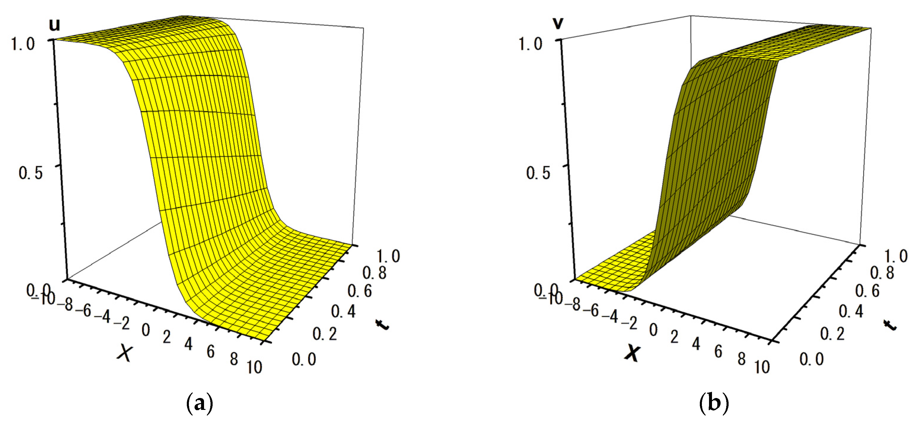
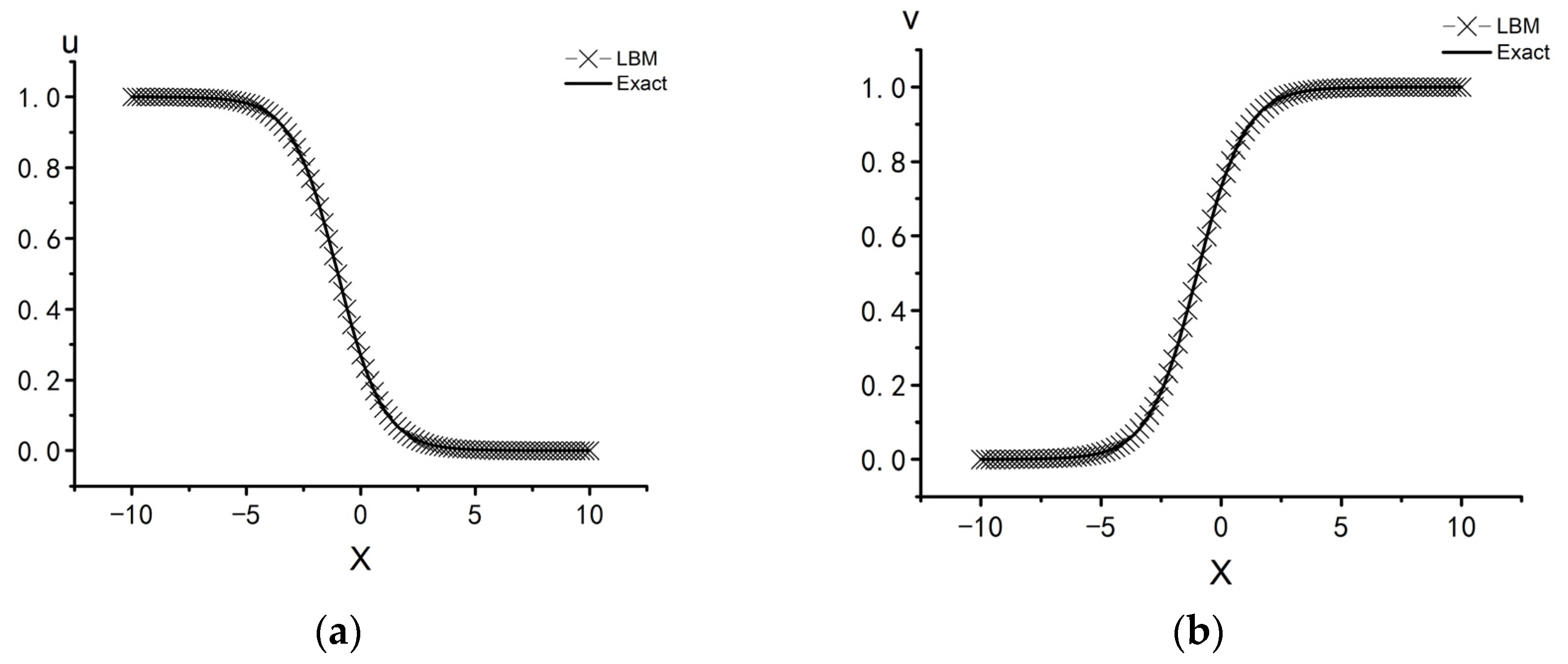
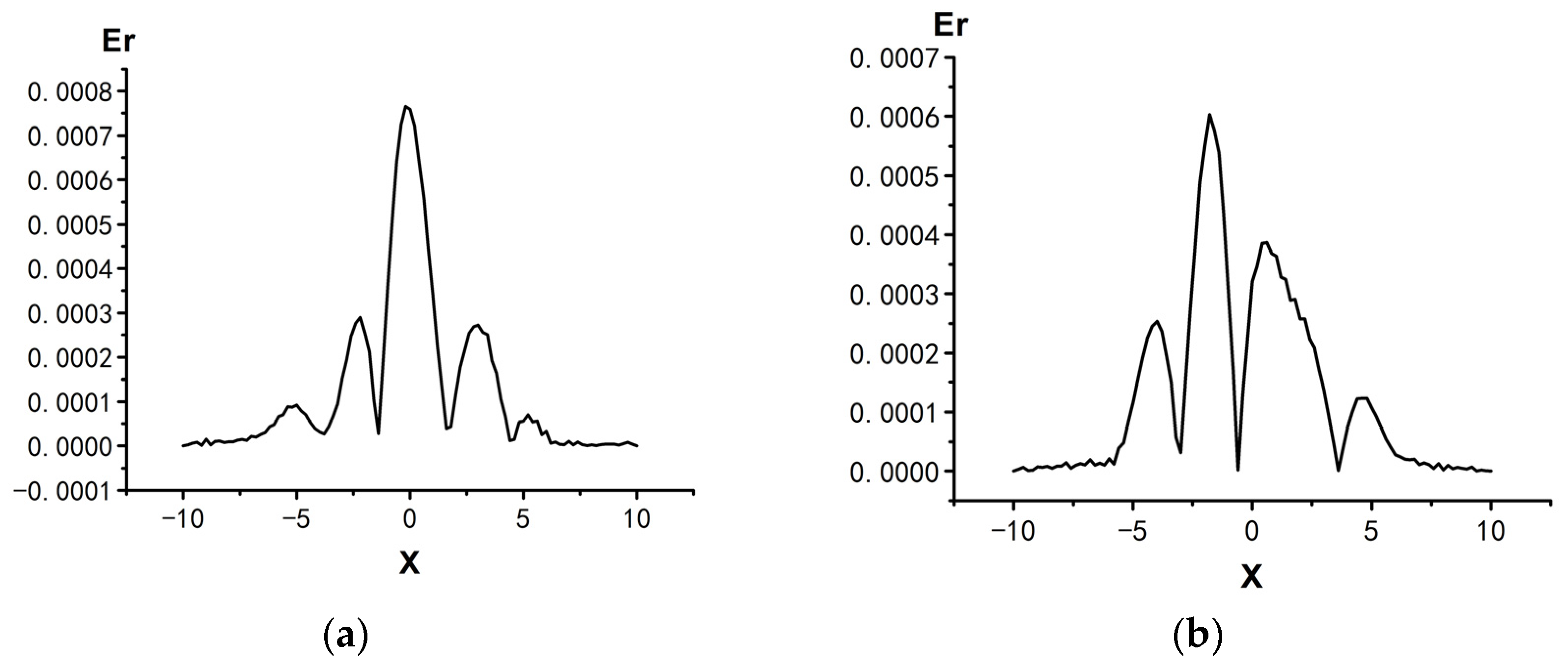
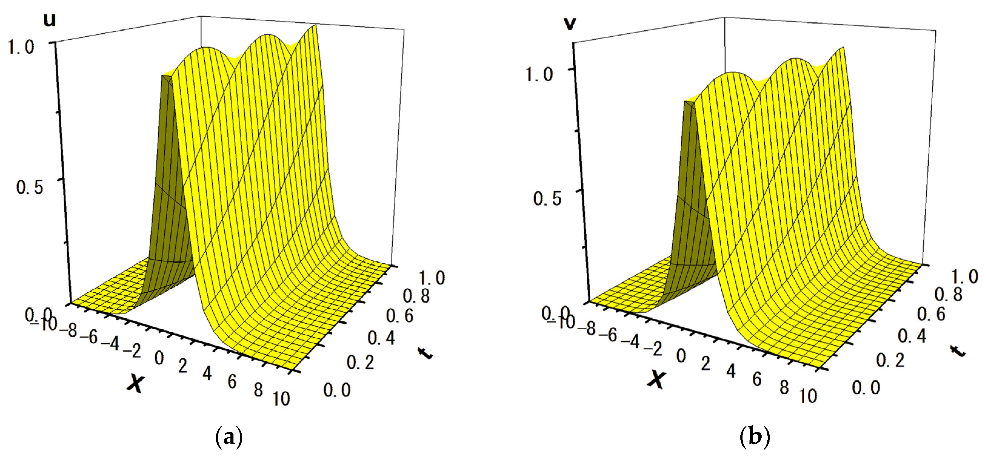
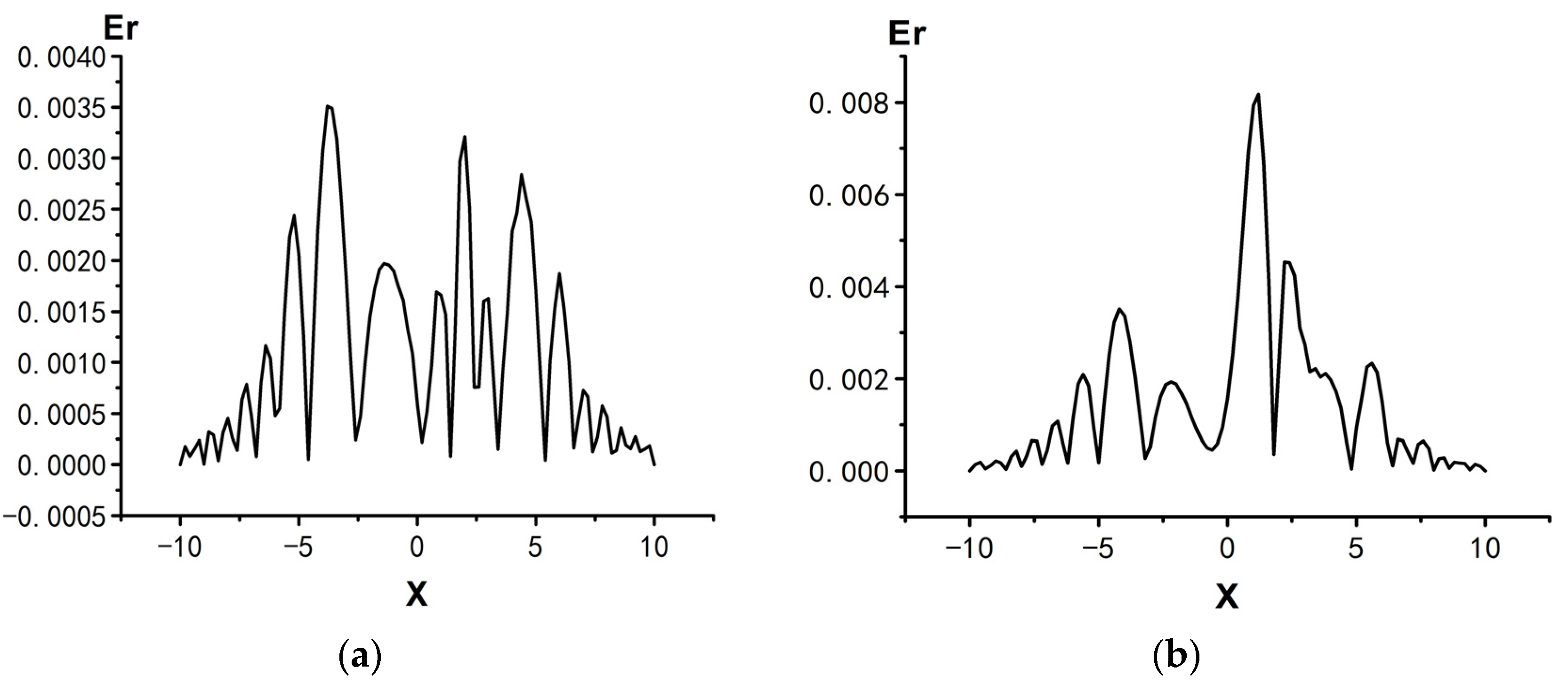
3.1.2. Numerical Simulation of Wave Propagation

In this part, we will provide numerical examples of the variable coefficient nonlinear Schrödinger Equations (4) and (5).

Case I in this example, $\lambda (x,t)=1$, $\beta =2$, and $\gamma (x,t)=-1$, refer to [2], and the exact solution is

$$u(x,t)={\displaystyle \frac{u_0}{1+\exp [\sqrt{\lambda }x+(\beta \sqrt{\lambda }-\lambda )t+x_0]}},$$

(26)

$$v(x,t)={\displaystyle \frac{u_0\exp [\sqrt{\lambda }x+(\beta \sqrt{\lambda }-\lambda )t+x_0]}{1+\exp [\sqrt{\lambda }x+(\beta \sqrt{\lambda }-\lambda )t+x_0]}},$$

(27)

The initial condition and the boundary condition are given according to the exact solution

$$u(x,0)={\displaystyle \frac{u_0}{1+\exp [\sqrt{\lambda }x+x_0]}},-10\le x\le 10,$$

(28)

$$v(x,0)={\displaystyle \frac{u_0\exp [\sqrt{\lambda }x+x_0]}{1+\exp [\sqrt{\lambda }x+x_0]}},-10\le x\le 10.$$

(29)

The boundary conditions are

$$u(x_B,t)={\displaystyle \frac{u_0}{1+\exp [\sqrt{\lambda }{x}_B+(\beta \sqrt{\lambda }-\lambda )t+x_0]}},t>0.$$

(30)

$$v(x_B,t)={\displaystyle \frac{u_0\exp [\sqrt{\lambda }{x}_B+(\beta \sqrt{\lambda }-\lambda )t+x_0]}{1+\exp [\sqrt{\lambda }{x}_B+(\beta \sqrt{\lambda }-\lambda )t+x_0]}},t>0.$$

(31)

where $x_B$ represents the boundary point, $u_0^2=-{\displaystyle \frac{\lambda }{\gamma }}$, $x_0=0$. The calculation interval is $[-10,10]$. The computational parameters are the number of lattices $M=101$, $\Delta t=0.001$, $\Delta x=0.02$, and $\tau =1.021$. We use the software Fortran Powerstation 4.0 to write code for numerical operations, and the numerical results are shown in Figure 2, Figure 3, Figure 4, Figure 5 and Figure 6. Figure 2 shows the wave propagation simulated by the lattice Boltzmann method. Figure 3 shows the comparison between the lattice Boltzmann solution and the exact solution. Figure 4 shows the error curves, $Er=\left|u^N-u^E\right|$ and $\left|v^N-v^E\right|$, where $u^N$ and $v^N$ represent the lattice Boltzmann solution, and $u^E$ and $v^E$ represent the exact solution. The results show that the lattice Boltzmann solution agrees with the exact solution. We use the infinite norm of error of $u$, ${‖Er‖}_{\infty }=\max \left\{Er\right\}=\max \left\{\left|u^N-u^E\right|\right\}$, to evaluate the performance of the constructed lattice Boltzmann model. Figure 5 shows the relationship between the infinite norm of error ${‖Er‖}_{\infty }$ and the Knudsen coefficient ε. Through linear fitting, the fitted line is obtained, ${\log }_{10}(|\left|Er\right|{|}_{\infty })=1.5174\times {\log }_{10}\epsilon +0.58836$. The slope of the straight line represents the order of convergence of the model, and the results show that the constructed model is convergent. In the lattice Boltzmann model, ε is equal to the time step Δt and the spatial step Δx = cΔt = cε. For a fixed parameter c, the order of convergence of the model in both time and space is 1.5174. Figure 4 also shows the relationship between the truncation error and the Knudsen number.

To verify the effectiveness of our lattice Boltzmann model, we compared our model with several classical schemes. The comparison results are shown in Figure 6 and

Table 1. Comparison table of different schemes.

Scheme		Time t = 0.2	Time t = 0.4	Time t = 0.6	Time t = 0.8	Time t = 1.0
Classic Explicit Scheme	${‖Er‖}_{\infty }$	2.236962 × 10−4	3.646016 × 10−4	6.057620 × 10−4	8.040071 × 10−4	9.397864 × 10−4
	CPU Time (s)	0.094	0.213	0.259	0.263	0.310
Three-Level Explicit Scheme	${‖Er‖}_{\infty }$	3.236234 × 10−4	6.066561 × 10−4	8.515120 × 10−4	1.037896 × 10−3	1.171649 × 10−3
	CPU Time (s)	0.133	0.232	0.268	0.284	0.311
Hopscotch Scheme	${‖Er‖}_{\infty }$	3.938675 × 10−4	7.615089 × 10−4	1.185596 × 10−3	1.506567 × 10−3	1.693845 × 10−3
	CPU Time (s)	0.132	0.241	0.297	0.325	0.388
LBM	${‖Er‖}_{\infty }$	1.530647 × 10−4	2.858341 × 10−4	5.033910 × 10−4	6.718934 × 10−4	7.652342 × 10−4
	CPU Time (s)	0.078	0.140	0.171	0.188	0.203

. Figure 6a shows the comparison of solitary waves simulated by these different schemes, and Figure 6b shows the error comparison of these schemes. It can be seen from the results that our lattice Boltzmann model error is lower than that of other schemes. We also compared the errors and time consumption of different schemes, and the results are listed in Table 1. From the data in Table 1, it can be seen that compared with other classic schemes, our lattice Boltzmann method exhibits advantages in both accuracy and time consumption.

Case II In this example, $\lambda (x,t)=1$, $\beta =1$, $\gamma (x,t)=-1$. The initial conditions are

$$u(x,0)={\displaystyle \frac{u_0\exp [\sqrt{\lambda }x+x_0]}{1+\exp [\sqrt{\lambda }x+x_0]}},-10\le x\le 10,$$

(32)

$$v(x,0)={\displaystyle \frac{u_0}{1+\exp [\sqrt{\lambda }x+x_0]}},-10\le x\le 10.$$

(33)

The boundary conditions are

$$u(x_B,t)={\displaystyle \frac{u_0\exp [\sqrt{\lambda }{x}_B+(\beta \sqrt{\lambda }+\lambda )t+x_0]}{1+\exp [\sqrt{\lambda }{x}_B+(\beta \sqrt{\lambda }+\lambda )t+x_0]}},t>0.$$

(34)

$$v(x_B,t)={\displaystyle \frac{u_0}{1+\exp [\sqrt{\lambda }{x}_B+(\beta \sqrt{\lambda }+\lambda )t+x_0]}},t>0.$$

(35)

where $x_B$ represents the boundary point, $u_0^2=-{\displaystyle \frac{\lambda }{\gamma }}$, $x_0=0$. The calculation interval is $[-10,10]$. The computational parameters are the number of lattices $M=101$, $\Delta t=0.001$, $\Delta x=0.02$, $\tau =0.944$, and the numerical results are shown in Figure 7, Figure 8 and Figure 9.

Case III In this example, $\lambda (x,t)=1$, $\beta =2$, $\gamma (x,t)=1$. The initial conditions are

$$u(x,0)=u_1\mathrm{sech}(a_1\sqrt{-\lambda }x+x_0),-10\le x\le 10,$$

(36)

$$v(x,0)=a_2{u}_1\mathrm{sech}(a_1\sqrt{-\lambda }(x+x_0),-10\le x\le 10,$$

(37)

The boundary conditions are

$$u(x_B,t)=u_1\mathrm{sech}(a_1\sqrt{-\lambda }{x}_B-a_1{a}_2\beta \sqrt{-\lambda }t+x_0),t>0.$$

(38)

$$v(x_B,t)=a_2{u}_1\mathrm{sech}(a_1\sqrt{-\lambda }(x_B-\beta a_{2}t+x_0)),t>0.$$

(39)

where $x_B$ represents the boundary point, $a_1=1$, $a_2=1$, $u_1=1$. The calculation interval is $[-10,10]$. The computational parameters are the number of lattices $M=101$, $\Delta t=0.001$, $\Delta x=0.02$, $\tau =0.96$, and the numerical results are shown in Figure 10, Figure 11 and Figure 12.

3.2. Variable Coefficient Fractional Order Nonlinear Schrödinger Equation

In this part, we consider constructing a lattice Boltzmann model for a class of variable coefficient fractional order nonlinear Schrödinger equation:

$$i{u}_t+\lambda (t){\displaystyle \frac{{\partial }^{\beta }u}{\partial |x{|}^{\beta }}}+v(x)u+\gamma (t){|u|}^{2}u=0, \mathrm{a}\le \mathrm{x}\le b,0\le t\le T.$$

(40)

where $u(x,t)$ is a complex valued wave function; $\lambda (t)$, $v(x)$, and $\gamma (t)$ are bounded real functions; $1<\beta \le 2,$ ${\displaystyle \frac{{\partial }^{\beta }u}{\partial |x{|}^{\beta }}}$ is the Riesz fractional derivative of order $\beta$, defined through Riemann Liouville integration as

$${\displaystyle \frac{{\partial }^{\beta }u}{\partial |x{|}^{\beta }}}=-\theta (I_{+}^{-\beta }+I_{-}^{-\beta })u.$$

(41)

where $\theta ={\displaystyle \frac{1}{2\cos (\beta \pi /2)}}$, $I_{\pm }^{-\beta }={\displaystyle \frac{{\partial }^2}{\partial x^2}}{I}_{\pm }^{2-\beta }u(x,t)$. According to Riemann Liouville’s integral definition, it can be inferred that

$$\left(I_{+}^{2-\beta }u\right)(x,t)={\displaystyle \frac{1}{\mathsf{\Gamma }(2-\beta )}}{\displaystyle {\int }_a^x{(x-\xi )}^{1-\beta }u(\xi ,t)d\xi ,}\hspace{1em}x>a,$$

(42)

$$\left(I_{-}^{2-\beta }u\right)(x,t)={\displaystyle \frac{1}{\mathsf{\Gamma }(2-\beta )}}{\displaystyle {\int }_x^b{(\xi -x)}^{\beta -1}u(\xi ,t)d\xi ,}\hspace{1em}x<b.$$

(43)

Therefore, Equation (40) can be expressed in the following form:

$$i{u}_t-\lambda (t)\theta {\displaystyle \frac{{\partial }^2}{\partial x^2}}(I_{+}^{2-\beta }+I_{-}^{2-\beta })u+v(x)u+\gamma (t){\mathsf{\left|}u\mathsf{\right|}}^{2}u=0, \mathrm{a}\le \mathrm{x}\le b,0\le t\le T.$$

(44)

Next, We will use the series of equations at different time scales to recover Equation (44).

3.2.1. Recovery of Macroscopic Equation

We define the macroscopic quantity $u$ as

$$iu={\displaystyle \sum _{\alpha }{f}_{\alpha }(x,t)}.$$

(45)

Here, component number $\sigma =1$ is omitted and not written. According to conservation condition ${\displaystyle \sum _{\alpha }f(x,t)}={\displaystyle \sum _{\alpha }{f}_{\alpha }^{eq}}(x,t)$, it can be concluded that

$$iu={\displaystyle \sum _{\alpha }{f}_{\alpha }^{(0)}(x,t)},$$

(46)

let the moments of the equilibrium distribution function be

$$m^0={\displaystyle \sum _{\alpha }{f}_{\alpha }^{(0)}}{e}_{\alpha }=0,$$

(47)

$${\pi }^0={\displaystyle \sum _{\alpha }{f}_{\alpha }^{(0)}}{e}_{\alpha }^2=-{\displaystyle \frac{\lambda (t)\theta }{\epsilon C_2}}{I}_{\pm }^{2-\beta }u.$$

(48)

where the Riemann–Liouville integral $I_{\pm }^{2-\beta }u$ can be approximately calculated based on the Grünwald–Letnikov fractional derivative definitions on the left and right sides,

$$I_{+}^{2-\beta }u(x,t)\approx h^{2-\beta }{\displaystyle \sum _{r=0}^{\left[\frac{x-a}{h}\right]}\left[\begin{array}{c}2-\beta \\ r\end{array}\right]}u(x-rh,t),\hspace{1em}a<x<b,$$

(49)

$$I_{-}^{2-\beta }u(x,t)\approx h^{2-\beta }{\displaystyle \sum _{r=0}^{\left[\frac{b-x}{h}\right]}\left[\begin{array}{c}2-\beta \\ r\end{array}\right]}u(x+rh,t),\hspace{1em}a<x<b.$$

(50)

where $\left[\begin{array}{c}2-\beta \\ r\end{array}\right]={\displaystyle \frac{(2-\beta )(2-\beta +1)\cdots (2-\beta +r-1)}{r!}},$ for $r>0,$ and $\left[\begin{array}{c}2-\beta \\ r\end{array}\right]=1,$ for r = 0.

Assuming that ${\mathsf{\Omega }}_{\alpha }={\epsilon }^2{\mathsf{\Omega }}_{\alpha }^{(2)}$, i.e., ${\mathsf{\Omega }}_{\alpha }^{(n)}=0$, $n\ne 2.$ Then, from ${\displaystyle \sum _{\alpha }\left[(\mathrm{A}7)+\epsilon \times (\mathrm{A}8)\right]}$, it can be concluded that

$$i{u}_t-\lambda (t)\theta {\displaystyle \frac{{\partial }^2}{\partial x^2}}(I_{+}^{2-\beta }+I_{-}^{2-\beta })u=\epsilon {\displaystyle \sum _{\alpha }{\mathsf{\Omega }}_{\alpha }^{\left(2\right)}}+O({\epsilon }^2).$$

(51)

Equation (51) is an approximate formula for the recovered macroscopic Equation (44). We set

$${\displaystyle \sum _{\alpha }{\mathsf{\Omega }}_{\alpha }^{(2)}}=-V(x)u-\gamma (t){\left|u\right|}^{2}u,$$

(52)

If it is assumed that ${\mathsf{\Omega }}_{\alpha }^{(2)}$ is independent of $\alpha$, combining the D1Q3 model we can obtain

$${\mathsf{\Omega }}_{\alpha }^{(2)}={\mathsf{\Omega }}^{(2)}={\displaystyle \frac{-V(x)u-\gamma (t){\left|u\right|}^{2}u}{3\epsilon }}.$$

(53)

Solving Equations (46)–(48), the equilibrium distribution function is obtained

$$f_{\alpha }^{(0)}=\left\{\begin{array}{ll}{\displaystyle \frac{-\lambda (t)\theta }{2c^2\epsilon C_2}}(I_{+}^{2-\beta }+I_{-}^{2-\beta })u,& \alpha =1,2 ,\hfill \\ iu-2f_1^{(0)},& \alpha =0.\hfill \end{array}\right.$$

(54)

Summing ${\left(\mathrm{A}7\right)+\mathsf{\epsilon }\text{×}\left(\mathrm{A}8\right)+\mathsf{\epsilon }}^2\text{×}\left(\mathrm{A}9\right)$ over $\alpha$ yields

$$i{u}_t-\lambda (t)\theta {\displaystyle \frac{{\partial }^2}{\partial x^2}}(I_{+}^{2-\beta }+I_{-}^{2-\beta })u=\epsilon {\displaystyle \sum _{\alpha }{\mathsf{\Omega }}_{\alpha }^{\left(2\right)}}+E_2+O({\epsilon }^3).$$

(55)

$E_2$ is the second-order error term. Through error analysis, it can be obtained that

$$\begin{array}{l}{E}_2=-{\epsilon }^2\left(C_3{\displaystyle \sum _{\alpha }{\Delta }^3}{f}_{\alpha }^{(0)}+2C_2{\displaystyle \sum _{\alpha }\Delta }{\displaystyle \frac{\partial }{\partial t_1}}{f}_{\alpha }^{(0)}+\tau {\displaystyle \sum _{\alpha }\Delta }{\mathsf{\Omega }}_{\alpha }^{(2)}\right)\\ \hspace{1em}=-{\displaystyle \frac{3\epsilon C_3\gamma }{C_2}}{\displaystyle \frac{{\partial }^3}{\partial t_0\partial x^2}}\left[I_{+}^{2-\beta }u(x,t)+I_{-}^{2-\beta }u(x,t)\right]\end{array}.$$

(56)

Thus, the macroscopic Equation (44) is recovered as

$$i{u}_t-\lambda (t)\theta {\displaystyle \frac{{\partial }^2}{\partial x^2}}(I_{+}^{2-\beta }+I_{-}^{2-\beta })u+v(x)u+\gamma (t){\left|u\right|}^{2}u=O(\epsilon ).$$

(57)

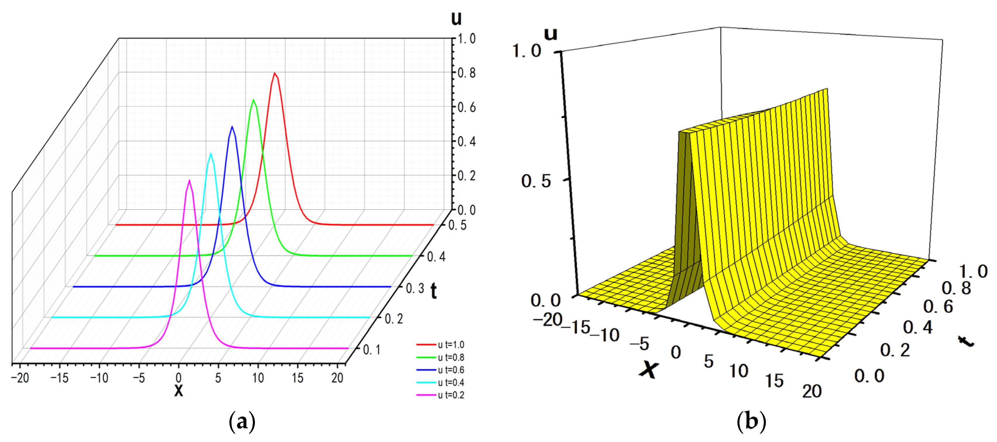
3.2.2. Numerical Example

We will numerically simulate the wave propagation of the equation in this section. A numerical example is given, $\lambda (t)=t/30$, $v(x)=\sin x$, $\gamma (t)=t/8$.

The initial conditions and the boundary conditions in this example are [21] as follows:

$$u(x,0)=\mathrm{sech}(x)\cdot \exp (2ix),-20\le x\le 20,$$

(58)

$$u(-20,t)=u(20,t)=0. 0\le t\le 1.$$

(59)

The computational parameters are the number of lattices, $M=101$, $\Delta t=0.001$, $\Delta x=0.02$, $c=\Delta x/\Delta t$, $\tau =1.0755$. The propagation of the solitary wave solution using the lattice Boltzmann method for $\alpha =1.2, 1.4, 1.6, 1.8$ from $t=0$ to $t=0.5$ is shown in Figure 13, Figure 14, Figure 15 and Figure 16.

4. Conclusions

In this paper, we use the lattice Boltzmann method to numerically simulate wave propagation based on the variable coefficient nonlinear Schrödinger equation and the variable coefficient fractional order Schrödinger equation.

Lattice Boltzmann models are constructed for the two types of equations, a series of partial differential equations on different time scales are obtained by using the Taylor expansion, the Chapman–Enskog expansion, and the time multiscale expansion based on the basic Lattice Boltzmann equation. The macroscopic equations are recovered by choosing appropriate expressions for the moments of the equilibrium distribution function.

The solutions of the equations are numerically simulated together with numerical examples. By comparing the lattice Boltzmann solution with the exact solution and combining it with the error analysis, it is found that the lattice Boltzmann solution agrees with the exact solution. Furthermore, the effectiveness of our method was verified by comparing the lattice Boltzmann model with other classical schemes. The comparison results indicate that our method has shown advantages in both computational accuracy and time consumption. The convergence of the model has also been numerically verified.

The research results indicate that the lattice Boltzmann method is effective in studying wave propagation based on the variable coefficient nonlinear Schrödinger equation and the variable coefficient fractional order Schrödinger equation. These two types of equations are of great research value in various fields, so this work investigates the strong research significance of the lattice Boltzmann method for solving the solitary wave solutions of these two types of equations. In our future work, we will further research a high-precision and high-efficiency numerical method.

References

1. Huang, F.T. Algorithm and Characterization of Optical Soliton Solutions for NLS Equations in Fiber Optic Communications; University of Science and Technology Beijing: Beijing, China, 2023. [Google Scholar]
2. Chen, X.W. A Study of the Soliton Solution of the Schrödinger Equation with Variable Coefficients; Nanjing University of Information Engineering: Nanjing, China, 2018. [Google Scholar]
3. Wen, S.T.; Manafian, J.; Sedighi, S.; Atmaca, S.P.; Gallegos, C.; Mahmoud, K.H.; Alsubaie, A.S.A. Interactions among lump optical solitons for coupled nonlinear Schrödinger equation with variable coefficient via bilinear method. Sci. Rep. 2024, 14, 19568. [Google Scholar] [CrossRef] [PubMed]
4. Song, N.; Liu, R.; Guo, M.M.; Ma, W.X. Nth order generalized Darboux transformation and solitons, breathers and rogue waves in a variable-coefficient coupled nonlinear Schrödinger equation. Nonlinear Dynam. 2023, 111, 19347–19357. [Google Scholar] [CrossRef]
5. Gu, Y.; Chen, B.; Ye, F.; Aminakbari, N. Soliton solutions of nonlinear Schrödinger equation with the variable coefficients under the influence of Woods–Saxon potential. Results Phys. 2022, 42, 105979. [Google Scholar] [CrossRef]
6. Hong, B. Exact solutions for the conformable fractional coupled nonlinear Schrödinger equations with variable coefficients. J. Low Freq. Noise Vib. Act. Control 2023, 42, 628–641. [Google Scholar] [CrossRef]
7. Yu, F.; Li, L. Soliton robustness, interaction and stability for a variable coefficients Schrödinger(VCNLS) equation with inverse scattering transformation. Chaos Soliton. Fract. 2024, 185, 115185. [Google Scholar] [CrossRef]
8. Yin, H.M.; Tian, B.; Chai, J.; Liu, L.; Sun, Y. Numerical solutions of a variable-coefficient nonlinear Schrödinger equation for an inhomogeneous optical fiber. Comput. Math. Appl. 2018, 76, 1827–1836. [Google Scholar] [CrossRef]
9. Tay, K.G.; Choy, Y.Y.; Tionng, W.K.; Ong, C.T. Numerical solutions of the dissipative nonlinear Schrödinger equation with variable coefficient arises in elastic tube. Dyn. Contin. Discret. Impuls. Syst. Ser. B. Appl. Algorithms 2018, 25, 53–61. [Google Scholar]
10. Sun, J.; Dong, H.; Liu, M.; Fang, Y. Data-driven rogue waves solutions for the focusing and variable coefficient nonlinear Schrödinger equations via deep learning. Chaos 2024, 34, 073134. [Google Scholar] [CrossRef] [PubMed]
11. Qian, Y.H.; d’Humieres, D.; Lallemand, P. Lattice BGK Models for Navier- Stokes Equations. Europhys. Lett. 1992, 17, 479–484. [Google Scholar] [CrossRef]
12. Chen, S.Y.; Doolen, G.D. Lattice Boltzmann method for fluid flows. Annu. Rev. Fluid Mech. 1998, 30, 329–364. [Google Scholar] [CrossRef]
13. Succi, S.; Benzi, R. Lattice Boltzmann equation for quantum mechanics. Phys. D Nonlinear Phenom. 1993, 69, 327–332. [Google Scholar] [CrossRef]
14. He, Y.B.; Lin, X.Y. Numerical analysis and simulations for coupled nonlinear Schrödinger equations based on lattice Boltzmann method. Appl. Math. Lett. 2020, 106, 106391. [Google Scholar] [CrossRef]
15. Shi, B.C.; Guo, Z.L. Lattice Boltzmann model for nonlinear convection-diffusion equations. Phys. Rev. E 2009, 79, 016701. [Google Scholar]
16. Nie, X.B.; Doolen, G.D.; Chen, S.Y. Lattice-Boltzmann Simulations of Fluid Flows in MEMS. J. Stat. Phys. 2002, 107, 279–289. [Google Scholar] [CrossRef]
17. Lallemand, P.; Luo, L.S. Lattice Boltzmann equation with Overset method for moving objects in two-dimensional flows. J. Comput. Phys. 2020, 407, 109223. [Google Scholar] [CrossRef]
18. Dubois, F.; Lallemand, P.; Tekitek, M.M. On anti bounce back boundary condition for lattice Boltzmann schemes. Comput. Math. Appl. 2019, 79, 555–575. [Google Scholar] [CrossRef]
19. Boghosian, B.M.; Dubois, F.; Lallemand, P. Numerical approximations of a lattice Boltzmann scheme with a family of partial differential equations. Comput. Fluids 2024, 284, 106410. [Google Scholar] [CrossRef]
20. Wang, H.M. A lattice Boltzmann model for the ion- and electron-acoustic solitary waves in beam-plasma system. Appl. Math. Comput. 2016, 279, 62–75. [Google Scholar] [CrossRef]
21. Shen, H. Finite difference study of Schrödinger equation with variable coefficients of fractional order. J. Ningxia Norm. Coll. 2023, 44, 27–34. [Google Scholar]
Figure 1. D1Q3 model.
Mathematics 12 03807 g001
Figure 2. Wave propagation simulated by the lattice Boltzmann method. (a) Wave of u ; (b) wave of v .
Mathematics 12 03807 g002
Figure 3. Comparison of the lattice Boltzmann solution and exact solution, t = 1.0 . (a) Wave solution of u ; (b) wave solution of v .
Mathematics 12 03807 g003
Figure 4. Error curve, t = 1.0 . (a) Error curve of u ; (b) error curve of v .
Mathematics 12 03807 g004
Figure 5. Infinite method of error E r versus Knudsen number curve.
Mathematics 12 03807 g005
Figure 6. Comparison of different schemes, t = 1.0 . (a) Wave solution of u ; (b) error curve of u .
Mathematics 12 03807 g006
Figure 7. Wave propagation simulated by the lattice Boltzmann method. (a) Wave of u ; (b) wave of v .
Mathematics 12 03807 g007
Figure 8. Comparison between the lattice Boltzmann solution and exact solution, t = 1.0 . (a) Wave solution of u ; (b) wave solution of v .
Mathematics 12 03807 g008
Figure 9. Error curve, t = 1.0 . (a) Error curve of u ; (b) error curve of v .
Mathematics 12 03807 g009
Figure 10. Wave propagation simulated by the lattice Boltzmann method. (a) Wave of u ; (b) wave of v .
Mathematics 12 03807 g010
Figure 11. Comparison of the lattice Boltzmann solution and exact solution, t = 1.0 . (a) Wave solution of u ; (b) wave solution of v .
Mathematics 12 03807 g011
Figure 12. Error curve, t = 1.0 . (a) Error curve of u ; (b) error curve of v .
Mathematics 12 03807 g012
Figure 13. Solitary wave propagation using the lattice Boltzmann method, α = 1.2 . (a) Waterfall plot; (b) solitary wave propagation.
Mathematics 12 03807 g013
Figure 14. Solitary wave propagation using the lattice Boltzmann method, α = 1.4 . (a) Waterfall plot; (b) solitary wave propagation.
Mathematics 12 03807 g014
Figure 15. Solitary wave propagation using the lattice Boltzmann method, α = 1.6 . (a) Waterfall plot; (b) solitary wave propagation.
Mathematics 12 03807 g015
Figure 16. Solitary wave propagation using the lattice Boltzmann method, α = 1.8 . (a) Waterfall plot; (b) solitary wave propagation.
Mathematics 12 03807 g016