Modified Wave-Front Propagation and Dynamics Coming from Higher-Order Double-Well Potentials in the Allen–Cahn Equations

Abstract

In this paper, we conduct a numerical investigation into the influence of polynomial order on wave-front propagation in the Allen–Cahn (AC) equations with high-order polynomial potentials. The conventional double-well potential in these equations is typically a fourth-order polynomial. However, higher-order double-well potentials, such as sixth, eighth, or any even order greater than four, can model more complex dynamics in phase transition problems. Our study aims to explore how the order of these polynomial potentials affects the speed and behavior of front propagation in the AC framework. By systematically varying the polynomial order, we observe significant changes in front dynamics. Higher-order polynomials tend to influence the sharpness and speed of moving fronts, leading to modifications in the overall pattern formation process. These results have implications for understanding the role of polynomial potentials in phase transition phenomena and offer insights into the broader application of AC equations for modeling complex systems. This work demonstrates the importance of considering higher-order polynomial potentials when analyzing front propagation and phase transitions, as the choice of polynomial order can dramatically alter system behavior.

1. Introduction

In this article, we numerically investigate the effect of polynomial order on front propagation in the Allen–Cahn (AC) equation with high-order polynomial potentials:

$$\begin{array}{ccc}\hfill {\displaystyle \frac{\partial u(\mathbf{x},t)}{\partial t}}& =& -{\displaystyle \frac{F_{\alpha }^{\prime }\left(u(\mathbf{x},t)\right)}{{ϵ}^2}}+\Delta u(\mathbf{x},t).\hfill \end{array}$$

(1)

Here, $u(\mathbf{x},t)$ is a phase field at $\mathbf{x}$ and time t, $ϵ$ is a parameter, and $F_{\alpha }\left(u\right)$ for $\alpha$ is given as follows:

$$\begin{array}{c}\hfill F_{\alpha }\left(u(\mathbf{x},t)\right)={\displaystyle \frac{1}{4{\alpha }^2}}{\left({\left(u(\mathbf{x},t)\right)}^{2\alpha }-1\right)}^2.\end{array}$$

(2)

The AC equation describes the process of phase separation in binary alloy systems and models the evolution of interfaces over time [1]. When the parameter $\alpha =1$,  Equation (3) reduces to the classical AC equation [2,3,4]. The AC equation presents numerous open problems in the areas of mathematics, computation, and physics. Mathematically important challenges include the rigorous derivation of mean curvature flow (MCF) in the sharp interface limit for complex geometries. The formation, propagation, and resolution of singularities remain poorly understood. Simulating the AC equation in high dimensions (i.e., the curse of dimensionality) with accurate interface resolution represents ongoing challenges. Coupling AC equations with physical processes, such as fluid flows or material heterogeneities, and incorporating experimental constraints into models require further exploration.

Equation (1) can be explicitly written as

$$\begin{array}{c}\hfill {\displaystyle \frac{\partial u(\mathbf{x},t)}{\partial t}}=-{\displaystyle \frac{1}{\alpha {ϵ}^2}}{\left(u(\mathbf{x},t)\right)}^{2\alpha -1}\left({\left(u(\mathbf{x},t)\right)}^{2\alpha }-1\right)+\Delta u(\mathbf{x},t).\end{array}$$

(3)

Figure 1a represents the function $F_{\alpha }\left(u\right)$ for different values of the parameter $\alpha$. The horizontal axis denotes u, ranging from −1.5 to 1.5, and the vertical axis represents $F_{\alpha }\left(u\right)$. The plot compares five different curves, each corresponding to different values of $\alpha$ (from 1 to 5): The black curve ($\alpha =1$) has the steepest gradients within the given range. As $\alpha$ increases from 2 to 5, the gradients of $F_{\alpha }\left(u\right)$ decrease, and the curve becomes flatter and less pronounced. Figure 1b shows the negative derivative of the function, $-F_{\alpha }^{\prime }\left(u\right)$, for the same values of $\alpha$ (1 through 5). The horizontal axis is, again, u, and the vertical axis represents the value of $-F_{\alpha }^{\prime }\left(u\right)$. The black curve for $\alpha =1$ shows a smooth negative sine-like wave. As $\alpha$ increases, the curve becomes flatter, particularly around $u=0$. The higher $\alpha$ values exhibit less variation in the derivative values compared to $\alpha =1$.

Equation (1) can be derived by the $L^2$-gradient flow of the following free energy functional:

$$\begin{array}{c}\hfill \mathcal{E}\left(u\right)={\int }_{\mathsf{\Omega }}\left({\displaystyle \frac{F_{\alpha }\left(u\right)}{{ϵ}^2}}+{\displaystyle \frac{1}{2}}{|\nabla u|}^2\right)\mathrm{d}\mathbf{x}.\end{array}$$

(4)

The AC equation is particularly important as a fundamental mathematical model in phase field approximation, providing insights into the dynamics of phase boundaries and interfaces in various physical systems. Due to its flexibility and wide-ranging applicability, the phase field method has become a fundamental tool in materials science and fluid dynamics [6,7], which enables insights into complex processes such as pattern formation, tumor growth simulation [8], classification, image processing [9], emotion classification [10], multi-phase image segmentation [11], phase transitions, and surface reconstruction [12]. Furthermore, it serves as a benchmark for physics-informed neural networks [13,14,15] and effectively models surface tension-driven phenomena, offering notable high precision [16]. Shah et al. [17] proposed a robust algorithm for solving the AC equation using a diagonally implicit fractional-step scheme for time discretization and FEMs for space and demonstrated the advantages of adaptive grids and comparing time discretization schemes for accuracy and computational efficiency. One of the important features of the AC equation is the maximum principle [18,19], which is very important. For instance,  Wang et al. [20] developed a novel, linear, energy-stable, and maximum principle-preserving method for numerically approximating the AC equation, and demonstrated improved stability and efficiency over traditional methods. Xie et al. [21] proposed an improved phase field method that eliminates curvature effects through a nonlinear preprocessing procedure, studying the impact of curvature effects on structural performance and effectively capturing shape details while countering the excessive smoothing effects of the phase field framework. Tan and Zhang [22] introduced a two-level linearized difference method for the AC equations, which satisfies the discrete maximum principle, energy stability, and second-order accuracy in time and space.

Deng and Zhao [23] proposed two energy-dissipation-preserving alternating-direction-implicit FDMs based on invariant energy quadratization methods for nonlinear energy dissipation systems, with the results demonstrating their accuracy and efficiency. Poochinapan and Wongsaijai [24] proposed a fourth-order compact FDM with a stabilization term for solving the AC equation in 1D and 2D, which preserves the energy-decaying property and achieves high accuracy for spatial and temporal discretizations. Ntsokongo [25] investigated the asymptotic behavior of an AC-type equation with temperature under Dirichlet boundary conditions and demonstrated well-posedness, the existence of a finite-dimensional global attractor, and exponential attractors. Nara [26] studied the long-term behavior of solutions to the AC equation on ${\mathbb{R}}^n$ (with $n>2$) and showed that solutions develop a front that aligns with a spreading sphere governed by mean curvature   flow [27,28], with distances converging to a constant in each radial direction over time. Li et al. [29] explored the application of a multi-component system on surfaces using a direct discretization method that is unconditionally stable in first- and second-order conditions, with good stability and precision.

The main purpose of this paper is to investigate the influence of different polynomial orders on front propagation dynamics in the AC equations, particularly focusing on how higher-order polynomial potentials affect the speed, sharpness, and behavior of moving fronts in phase transition problems, providing insights into the broader application of these equations in modeling complex systems.

The outline of this paper is as follows. Section 2 provides a detailed explanation of the numerical method employed to solve the AC equation, specifically focusing on cases with high-order polynomial free energy potentials. This section outlines the algorithmic approach and its relevance to the problem at hand. Section 3 presents the results of various computational experiments, demonstrating the practical application and effectiveness of the proposed method in capturing the front propagation dynamics influenced by different polynomial orders. Lastly, Section 5 offers a comprehensive conclusion, summarizing the key findings of the study and discussing their broader implications, as well as potential directions for future research.

2. Numerical Methods

For simplicity and to focus on the effects of high-order polynomials on the speed and behavior of front propagation in the AC framework, we used a fully explicit numerical method. It is noted that we may use the Fourier spectral method [30] to solve the equation. First, we consider a numerical scheme in one-dimensional (1D) space. Let $\mathsf{\Omega }=(L_x,R_x)$ and ${\mathsf{\Omega }}_h=\left\{x_i\right|x_i=L_x+(i-0.5)h,1\le i\le N_x\}$, where h is the step size and $N_x$ is an integer. Let $u_i^n=u(x_i,n\Delta t)$ and ${\displaystyle \parallel {\mathbf{u}}^n{\parallel }_{\infty }=\underset{1\le i\le N_x}{max}\left|u_i^n\right|}$, where ${\mathbf{u}}^n=(u_1^n,u_2^n,\dots ,u_{N_x}^n)$. The AC model (1) is discretized using an explicit method as follows:

$$\begin{array}{c}\hfill {\displaystyle \frac{u_i^{n+1}-u_i^n}{\Delta t}}={\displaystyle \frac{{\left(u_i^n\right)}^{2\alpha -1}\left(1-{\left(u_i^n\right)}^{2\alpha }\right)}{\alpha {ϵ}^2}}+{\displaystyle \frac{u_{i+1}^n-4u_i^n+u_{i-1}^n}{h^2}}.\end{array}$$

(5)

Then, the fully explicit 1D discrete updating scheme is as follows:

$$\begin{array}{ccc}\hfill u_i^{n+1}& =& u_i^n+\Delta t\left({\displaystyle \frac{{\left(u_i^n\right)}^{2\alpha -1}\left(1-{\left(u_i^n\right)}^{2\alpha }\right)}{\alpha {ϵ}^2}}+{\displaystyle \frac{u_{i+1}^n-4u_i^n+u_{i-1}^n}{h^2}}\right),\hfill \end{array}$$

(6)

$$\begin{array}{ccc}\hfill u_0^n& =& u_1^n\mathrm{and}{u}_{N_x+1}^n=u_{N_x}^n.\hfill \end{array}$$

(7)

Next, we consider a numerical scheme in two-dimensional (2D) space. Let $\mathsf{\Omega }=(L_x,R_x)\times (L_y,R_y)$ and ${\mathsf{\Omega }}_h=\left\{(x_i,y_j)\right|x_i=L_x+(i-0.5)h,y_j=L_y+(i-0.5)h,1\le i\le N_x,1\le j\le N_y\}$. Let $u_{ij}^n=u(x_i,y_j,n\Delta t)$ and ${\displaystyle \parallel {\mathbf{u}}^n{\parallel }_{\infty }=\underset{1\le i\le N_x,1\le j\le N_y}{max}\left|u_{ij}^n\right|}$, where ${\mathbf{u}}^n=\left(u_{ij}^n\right)$, $1\le i\le N_x$, and $1\le j\le N_y$. The AC model (1) is discretized by using an explicit method as follows:

$$\begin{array}{c}\hfill {\displaystyle \frac{u_{ij}^{n+1}-u_{ij}^n}{\Delta t}}={\displaystyle \frac{{\left(u_{ij}^n\right)}^{2\alpha -1}\left(1-{\left(u_{ij}^n\right)}^{2\alpha }\right)}{\alpha {ϵ}^2}}+{\displaystyle \frac{u_{i+1,j}^n+u_{i-1,j}^n+u_{i,j+1}^n+u_{i,j-1}^n-4u_{ij}^n}{h^2}}.\end{array}$$

(8)

Then, the fully explicit 2D discrete updating scheme is as follows:

$$\begin{array}{c}\hfill u_{ij}^{n+1}=u_{ij}^n+\Delta t\left({\displaystyle \frac{{\left(u_{ij}^n\right)}^{2\alpha -1}\left(1-{\left(u_{ij}^n\right)}^{2\alpha }\right)}{\alpha {ϵ}^2}}+{\displaystyle \frac{u_{i+1,j}^n+u_{i-1,j}^n+u_{i,j+1}^n+u_{i,j-1}^n-4u_{ij}^n}{h^2}}\right),\end{array}$$

(9)

where we use

$$\begin{array}{c}\hfill u_{i0}^n=u_{i1}^n,u_{i,N_y+1}^n=u_{i{N}_y}^n\mathrm{for} i=1,\dots ,N_x\mathrm{and}{u}_{0j}^n=u_{1j}^n,u_{N_x+1,j}^n=u_{N_{x}j}^n\mathrm{for} j=1,\dots ,N_y.\end{array}$$

For simplicity and to focus on the dynamics of the AC equation with high polynomial order, we use a fully explicit scheme. Alternative numerical methods, such as those based on radial basis functions [31], implicit methods [32], and highly accurate methods [33], may also be considered.

3. Numerical Simulations for One-Dimensional Domains

3.1. Equilibrium Solutions

We first consider equilibrium solutions. We investigate the relationship between the polynomial order parameter $\alpha$ and interfacial transition profiles. Let $u(x,0)$ be defined on $\mathsf{\Omega }=(-1,1)$ as follows:

$$\begin{array}{c}\hfill u(x,0)=\left\{\begin{array}{cc}-1,\hfill & \mathrm{if}x<0,\hfill \\ +1,\hfill & \mathrm{otherwise}.\hfill \end{array}\right.\end{array}$$

(10)

The numerical equilibrium solution, defined as ${\mathbf{u}}^{\infty }={\mathbf{u}}^{n+1}$, is computed using the numerical method that ensures the difference between successive iterations ${\mathbf{u}}^{n+1}$, and ${\mathbf{u}}^n$ remains smaller than a specified tolerance, $tol$, for some n, which is set to $tol={10}^{-11}$ in this study. That is, $\parallel {\mathit{u}}^{n+1}-{\mathit{u}}^n{\parallel }_{\infty }<tol$. Here, we use $N_x=200$, $ϵ=5h/\alpha$ and $\Delta t=0.9{ϵ}^2{h}^2/(2h^2+2{ϵ}^2)$, which guarantees numerical stability [34].

Figure 2a shows the equilibrium solutions ${\mathit{u}}^{\infty }$ for three different values of $\alpha$: 1, 2, and 5. The plot indicates how the polynomial order parameter $\alpha$ influences the transition profile of ${\mathit{u}}^{\infty }$. For $\alpha =1$, the blue dotted line shows a smoother transition between $-1$ and $+1$ across the domain. As $\alpha$ increases to 2 and 5 (represented by the red dashed line and black solid line, respectively), the transition profile becomes sharper. This indicates that higher-order polynomial potentials lead to a steeper gradient in the transition between phases. Figure 2b provides a magnified view of the transition region between the two equilibrium states of the solution, which focuses on the range $x\in [-0.2,0.2]$ for three different values of $\alpha$: 1, 2, and 5. This figure illustrates the effect of the polynomial order parameter $\alpha$ on the sharpness and nature of the interfacial transition in the equilibrium solution $u^{\infty }$. For $\alpha =1$ (blue dotted line), the transition from $u^{\infty }=-1$ to $u^{\infty }=+1$ occurs more gradually over a wider interval of x. This suggests a smoother, more diffuse interface between the two equilibrium states. The solution exhibits a less steep gradient in the transition zone, which indicates a more continuous and slow change between the two phases. For $\alpha =2$ (red dashed line), the transition becomes sharper compared to $\alpha =1$. The gradient in the transition region increases, which means the shift between the two phases happens over a shorter interval of x and creates a more distinct separation between the phases. The solution reflects a moderate sharpness in the interfacial region. For $\alpha =5$ (black solid line), the transition is the sharpest among the three values of $\alpha$. The gradient is steep, and the change from $u^{\infty }=-1$ to $u^{\infty }=+1$ occurs very rapidly, almost like a step function. This indicates that for higher values of $\alpha$, the system exhibits a very clear and abrupt phase separation, with the interface between the two phases becoming  extremely narrow.

As $\alpha$ increases, the transition region becomes more localized and sharper. For low values of $\alpha$ (e.g., $\alpha =1$), the transition between the two equilibrium states is smooth and spans a larger region, which means that the system has a more diffuse interface. In contrast, for higher values of $\alpha$ (e.g., $\alpha =5$), the transition is almost instantaneous, which results in a sharp, well-defined interface. This behavior demonstrates the impact of polynomial order on the steepness of phase boundaries within the system. These figures illustrate how different polynomial orders influence the equilibrium profile in the phase transition model.

3.2. Traveling Wave Solution

The traveling wave solution of the AC equation describes the movement of an interface between two stable phases, typically represented by a smooth wave profile that connects two equilibria. The wave moves at a constant speed c, and its shape remains fixed over time; see [5] for more details. The speed of the wave depends on the system’s parameters, including the potential function and the initial conditions. In practical applications, traveling wave solutions are crucial for understanding the dynamics of phase transitions and interface motion in various physical, chemical, and biological systems. Let us consider the following initial condition on $\mathsf{\Omega }=(0,3)$:

$$\begin{array}{c}\hfill u(x,0)=\left\{\begin{array}{cc}1,\hfill & \mathrm{if}x<0.2,\hfill \\ 0,\hfill & \mathrm{otherwise}.\hfill \end{array}\right.\end{array}$$

(11)

Here, we use $N_x=200$, $ϵ=h/\alpha$, and $\Delta t=0.9{ϵ}^2{h}^2/(2h^2+2{ϵ}^2)$, which guarantees numerical stability.

Figure 3 illustrates the traveling wave solutions of the AC equation at time $t=0.02$ for three different values of the parameter: $\alpha =1,2,$ and 5. The initial condition is also plotted for reference, which is a step function with a sharp transition from $u=1$ to $u=0$ at $x=0.2$, as represented by the magenta dotted line in the figure. For $\alpha =1$ (blue dotted line), this solution shows a more gradual transition between the two phases. The front has spread out, with a smooth transition zone between the regions where $u=1$ and $u=0$. This indicates that for lower values of $\alpha$, the traveling wave solution is less steep, and the interface between the phases is more diffuse. For $\alpha =2$ (red dashed line), the transition zone is sharper compared to $\alpha =1$. The wave-front becomes steeper, which means the transition between the two phases occurs more abruptly. This shows that increasing $\alpha$ sharpens the interface and makes the phase separation more distinct. For $\alpha =5$ (black solid line), this solution exhibits the steepest transition. The wave-front is almost vertical, indicating a very sharp interface between the two phases. For larger values of $\alpha$, the traveling wave becomes more like a step function, with minimal spreading in the transition zone. As $\alpha$ increases, the traveling wave solution becomes steeper when close to one value of the phase field. Around the neutral phase value, $u=0$, the transition profiles are similar for all considered $\alpha$ values.

3.3. Wave Propagation with Noise

Let $u(x,0)$ be defined on $\mathsf{\Omega }=(0,3)$ as follows:

$$\begin{array}{c}\hfill u(x,0)=\left\{\begin{array}{cc}1,\hfill & \mathrm{if}x<0.2,\hfill \\ 0.001\mathrm{rand}\left(x\right),\hfill & \mathrm{otherwise},\hfill \end{array}\right.\end{array}$$

(12)

where $\mathrm{rand}\left(x\right)$ is a random number between 0 and 1. Here, we use $N_x=200$, $ϵ=h/\alpha$, and $\Delta t=0.9{ϵ}^2{h}^2/(2h^2+2{ϵ}^2)$.

Figure 4 illustrates the wave propagation with initial noise over time for different values of the parameter $\alpha$ at three different times: $t=0.0008$, $0.0013$, and $0.025$. Figure 4a represents the wave propagation at an early time, $t=0.0008$. The initial condition shows a sharp drop at $x=0.2$. A noticeable noise has developed for $\alpha =1$ (blue dotted line), even though the initial noise level was small, with a maximum amplitude of $0.001$. This result indicates that smaller values of $\alpha$ are less effective in dampening the noise over time. The solutions for larger values of $\alpha$ ($\alpha =2$ and $\alpha =5$) show smoother behavior, with fewer oscillations compared to $\alpha =1$. This suggests that larger $\alpha$ values help to suppress the noise, leading to a smoother wave profile. Figure 4b corresponds to the wave propagation at $t=0.0013$. The noise for $\alpha =1$ is more evidently developed, while $\alpha =2$ and $\alpha =5$ show significantly less noisy behavior. Figure 4c shows the wave at $t=0.025$, a significantly later time than the previous two times. For $\alpha =1$ (blue dotted line), the solution has fully developed and reached the system’s maximum value. Both the $\alpha =2$ (red dashed line) and $\alpha =5$ (black solid line) cases still show propagation with damped noises. The former case evolves more rapidly than the latter case. By this time, the solutions for these cases have almost completely smoothed out the initial noise and resulted in a very stable and clean wave-front. This computational test illustrates wave propagation at different times and shows that smaller values of $\alpha$ (e.g., $\alpha =1$) are less effective in dampening noise, while larger values ($\alpha =2$ and $\alpha =5$) lead to smoother, more stable wave profiles as time progresses.

Let $u(x,0)$ be defined on $\mathsf{\Omega }=(0,3)$ with a higher noise level as follows:

$$\begin{array}{c}\hfill u(x,0)=\left\{\begin{array}{cc}1,\hfill & \mathrm{if}x<0.2,\hfill \\ 0.1\mathrm{rand}\left(x\right),\hfill & \mathrm{otherwise}.\hfill \end{array}\right.\end{array}$$

(13)

Figure 5 shows wave propagation under higher initial noise levels at three distinct times: $t=0.0005$, $0.0009$, and $0.025$, with parameter values $\alpha =1$, 2, and 5. Figure 5a shows the wave propagation at an early time, $t=0.0005$. For $\alpha =1$ (blue dotted line), a significant amount of developed noise is evident, with prominent oscillations. The larger values of $\alpha$ ($\alpha =2$ and $\alpha =5$) show smoother profiles, with $\alpha =5$ (black solid line) being the least affected by the initial noise. As in previous results, higher values of $\alpha$ lead to quicker damping of noise, resulting in more stable behavior. Figure 5b represents the wave propagation at a slightly later time, $t=0.0009$. The noise for $\alpha =1$ remains pronounced, and the oscillations are clearly visible. The solutions for $\alpha =2$ and $\alpha =5$ continue to show smoother behavior, with noise damping becoming more apparent. These results indicate that for larger $\alpha$, noise dissipation occurs faster, leading to a more stable solution.   Figure 5c corresponds to a significantly later time, $t=0.025$. By this time, for $\alpha =1$ (blue dotted line), the evolution reached an equilibrium constant state. For $\alpha =2$ (red dashed line), the noise is not fully damped, and the phase field extends ahead of the front with nonzero values. The solution for $\alpha =5$ (black solid line) has completely smoothed out the noise and resulted in a clean and stable wave-front. The difference in the behavior of the wave for the various $\alpha$ values highlights the role of $\alpha$ in noise suppression, with larger values of $\alpha$ producing a more robust damping effect.

This test demonstrates the effect of the parameter $\alpha$ on wave propagation in the presence of initially high noise. Larger values of $\alpha$ (such as $\alpha =5$) lead to faster suppression of noise and smoother wave profiles over time. Smaller values of $\alpha$ (such as $\alpha =1$) allow the noise to persist and indicate less effective damping. The progressive smoothing of the wave-front for higher $\alpha$ values, especially by the later time $t=0.025$, emphasizes the stabilizing influence of a larger $\alpha$ in wave propagation.

Let $u(x,0)$ be defined on $\mathsf{\Omega }=(0,3)$ with a higher noise level as follows:

$$\begin{array}{c}\hfill u(x,0)=\left\{\begin{array}{cc}1,\hfill & \mathrm{if}x<0.2,\hfill \\ -1,\hfill & \mathrm{if}x>2.8,\hfill \\ 0.1\left(2\mathrm{rand}\right(x)-1),\hfill & \mathrm{otherwise}.\hfill \end{array}\right.\end{array}$$

(14)

Figure 6 illustrates wave propagation in the presence of an initially higher noise level at three different times: $t=0.0001$, $0.002$, and $0.035$, for $\alpha =1$, 2, and 5. Figure 6a shows the wave propagation at an early time, $t=0.0001$. For $\alpha =1$ (blue dotted line), significant oscillations are already visible, showing that noise is strongly affecting the system. The amplitude of oscillations is large, extending throughout the domain. For $\alpha =2$ (red dashed line) and $\alpha =5$ (black solid line), the wave profiles are much smoother, with $\alpha =5$ showing the least amount of oscillation and noise. At this early time, the larger $\alpha$ values are clearly more effective at dampening the noise, leading to more stable wave-fronts. Figure 6b corresponds to the wave propagation at $t=0.002$. The initial noise for $\alpha =1$ develops substantially, with persistent oscillations throughout the domain. The wave shows strong disturbances, which indicates that smaller values of $\alpha$ allow the noise to develop more freely. For both $\alpha =2$ and $\alpha =5$, the noise is more dampened, and separation occurs from the neutral value. Figure 6c depicts wave propagation at a significantly later time, $t=0.035$. For $\alpha =1$, the oscillations persist. The wave is far from stable, and disturbances are prominent throughout the spatial domain. For both $\alpha =2$ and $\alpha =5$, the system has reached an equilibrium state, which separates the domain into regions of plus one and minus one, with a transition layer between these regions. The results indicate that the parameter $\alpha$ plays a critical role in controlling the damping of noise in wave propagation, with larger values leading to more complete noise suppression.

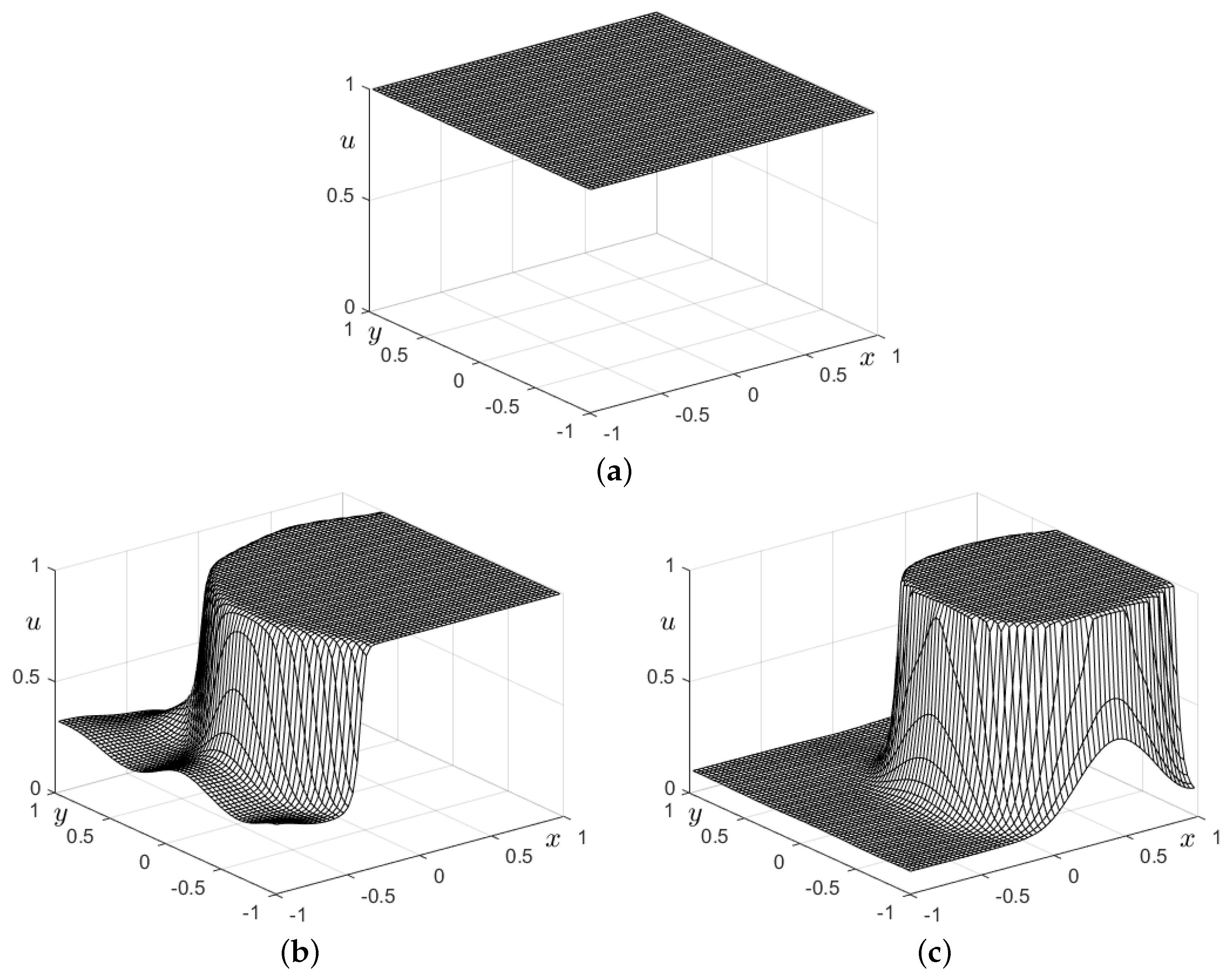
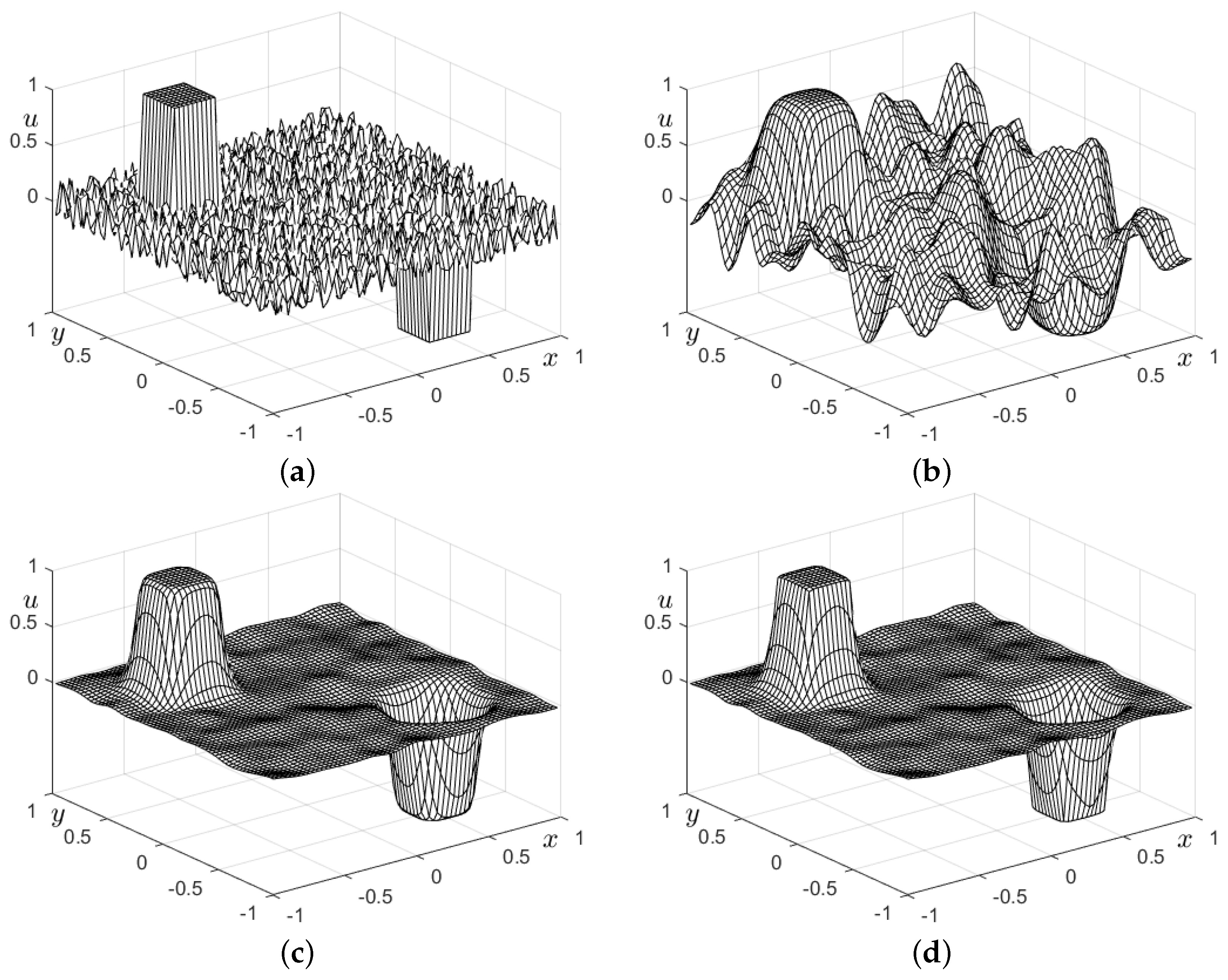
4. Numerical Simulations for Two-Dimensional Domain

In this section, numerical simulations are conducted on a two-dimensional domain, defined as $\mathsf{\Omega }=(-1,1)\times (-1,1)$. Let us consider the following initial condition with a higher noise level:

$$\begin{array}{c}\hfill u(x,y,0)=\left\{\begin{array}{cc}1,\hfill & \mathrm{if}0.2<x<0.7,-0.5<y<0,\hfill \\ 0.2\mathrm{rand}(x,y),\hfill & \mathrm{otherwise},\hfill \end{array}\right.\end{array}$$

(15)

where $\mathrm{rand}(x,y)$ is a random number between 0 and 1. Here, we use $N_x=64$, $ϵ=h/\alpha$, and $\Delta t=0.9{ϵ}^2{h}^2/(2h^2+4{ϵ}^2)$, which guarantees numerical stability.

Figure 7a represents the initial condition for $u(x,y,0)$. The graph shows a square structure with $u=1$ over a small region of the domain and noise in the remaining area. The region where $u=1$ is confined within $0.2<x<0.7$ and $-0.5<y<0$, while the other parts of the domain are randomly perturbed, generated by the function $0.1\times \mathrm{rand}(x,y)$. Figure 7b shows the result of the simulation at time $t=0.0025$ for $\alpha =1$. The initial sharp boundary of the block structure becomes smoother, and the noise increases gradually and smooths out, though the function still displays significant undulations. The diffusion process is apparent, and the block starts to lose its well-defined shape. Figure 7c presents the snapshot for $\alpha =2$ at the same time $t=0.0025$. Compared to Figure 7b, the surface appears smoother, which indicates a faster diffusion process relative to the growth of the noise. In Figure 7d, which is for $\alpha =5$, the noise has also smoothed out. At this early time, both $\alpha =2$ and $\alpha =5$ show similar behavior. The diffusion effect is very prominent here, with the surface approaching a more uniform structure. The higher value of $\alpha$ results in a more rapid spread of the initial noise, which makes for a more stabilized system compared to the $\alpha =1$ case.

Next, we conduct the simulation over a longer time period using the same initial conditions and parameter values. Figure 8 consists of three subplots (a–c), which display the results of simulations taken at a later time $t=0.022$ for different values of $\alpha =1$, 2, and 5, respectively. In Figure 8a, for $\alpha =1$, the surface is nearly flat, which indicates that the noise has fully developed and reached an equilibrium state with a value of 1. In Figure 8b, for ($\alpha =2$), in contrast to Figure 8a, the surface retains an interfacial transition layer within the domain. However, the noise has not fully disappeared and has continued to grow. In Figure 8c, for ($\alpha =5$), the surface in this plot shows an even more pronounced retention of the initial block structure compared to Figure 8b. The initial noise has flattened due to the diffusion process, while the initial block structure smoothly propagates outward, which is a good feature for data classification in the presence of noisy data, e.g., removing noise in fingerprint images. The simulation conducted over a longer time period for different values of $\alpha$ indicates that as $\alpha$ increases, the surface retains more of the initial block structure and smoothly propagates outward. A higher value, such as $\alpha =5$, preserves an interfacial transition layer and the propagation of the block structure, which could be advantageous for data classification in noisy conditions.

Let $u(x,y,0)$ be defined on $\mathsf{\Omega }=(-1,1)\times (-1,1)$ with a higher noise level as follows:

$$\begin{array}{c}\hfill u(x,y,0)=\left\{\begin{array}{cc}1,\hfill & \mathrm{if}|x+0.5|<0.15\mathrm{and} |y-0.5|<0.15,\hfill \\ -1,\hfill & \mathrm{if}|x-0.5|<0.15\mathrm{and} |y+0.5|<0.15,\hfill \\ 0.1\left(2\mathrm{rand}\right(x,y)-1),\hfill & \mathrm{otherwise}.\hfill \end{array}\right.\end{array}$$

(16)

Figure 9 shows the snapshots for different $\alpha$ values. Figure 9a shows the initial condition $u(x,y,0)$, which is defined in the domain $\mathsf{\Omega }=(-1,1)\times (-1,1)$, incorporating two square-like structures centered at $(-0.5,0.5)$ and $(0.5,-0.5)$. Outside these regions, the function $u(x,y,0)$ contains random noise scaled by $0.1$. The noise introduces high-frequency variations in the surface. In Figure 9b, for $\alpha =1$, we observe the evolution of the surface after some time has passed (time $t=0.003$) with $\alpha =1$. The noisy regions have grown, and they have started to smooth out significantly compared to the initial condition. The two central sharp structures have become less defined at the edges, though the overall form is retained. The surrounding region is much smoother, with fewer oscillations than the initial condition. In Figure 9c,d, for $\alpha =2$ and $\alpha =5$, the noise has reduced even more significantly. The surface is much smoother than in Figure 9b, which indicates a faster reduction of high-frequency components. The two sharp structures have become smoother at the edges. The evolution of the surface demonstrates how different values of $\alpha$ affect the dissipation of noise and the smoothing of the surface over time. Larger values of $\alpha$ result in faster smoothing and less prominent noisy fluctuations. The two distinct square regions remain but become progressively more blended with the background. Thus, it can be inferred that $\alpha$ controls the rate of smoothing or diffusion of the initial condition, with higher values leading to faster elimination of noise and a smoother overall surface.

Figure 10a–c show the evolutions of the system at a later time, $t=0.07$, for different values of $\alpha$ (1, 2, and 5, respectively). In Figure 10a, for $\alpha =1$, the system has evolved significantly, with the initial noise being smoothed out and random phase separation occurring under the influence of random noise. In Figure 10b,c, for $\alpha =2$ and $\alpha =5$, the surface has evolved further and exhibits sharper and more well-defined boundaries. The initially square structures expand outward and eventually meet along the diagonal line, dividing the domain into two distinct regions: one positive and the other negative.

5. Conclusions

In conclusion, our numerical investigation has demonstrated that the order of polynomial potentials significantly affects the behavior of front propagation in the AC equations. By exploring higher-order double-well potentials beyond the conventional fourth-order form, we have shown that these polynomials alter the sharpness and speed of moving fronts, which, in turn, modifies the pattern formation process during phase transitions. The results underscore the importance of selecting appropriate polynomial orders when modeling phase transition phenomena, as the dynamics and outcomes can be dramatically influenced by this choice. These findings provide a deeper understanding of the role of polynomial potentials in complex systems and suggest further research. Future work may focus on investigating the time-fractional AC equation [35], adaptive framework [36,37], the CH equation [38], and exploring curved surfaces within three-dimensional space [39]. Furthermore, research may extend these insights to other systems, such as the CH equation [40], thereby broadening the AC framework’s applicability in phase  transition modeling.

Finally, the key highlights of this study are as follows:

• The numerical investigation showed that the order of polynomial potentials significantly impacts wave-front propagation in the AC equations;
• Higher-order double-well potentials influence the wave-front moving under   noisy data;
• The study enhances our understanding of polynomial potentials in complex systems and suggests future research directions, including classification and noisy removal   image processing;
• Potential applications extend to other systems, broadening the AC framework’s relevance to phase transition modeling.

References

1. Shen, J.; Yang, X. Numerical approximations of Allen–Cahn and Cahn–Hilliard equations. Discrete Contin. Dyn. Syst. Ser. A 2010, 28, 1669–1691. [Google Scholar] [CrossRef]
2. Allen, S.M.; Cahn, J.W. A microscopic theory for antiphase boundary motion and its application to antiphase domain coarsening. Acta Metall. 1979, 27, 1085–1095. [Google Scholar] [CrossRef]
3. Singh, J.; Alshehri, A.M.; Momani, S.; Hadid, S.; Kumar, D. Computational analysis of fractional diffusion equations occurring in oil pollution. Mathematics 2022, 10, 3827. [Google Scholar] [CrossRef]
4. Lee, D. Gradient-descent-like scheme for the Allen–Cahn equation. AIP Adv. 2023, 13, 8. [Google Scholar] [CrossRef]
5. Zhai, S.; Feng, X.; He, Y. Numerical simulation of the three-dimensional Allen–Cahn equation by the high-order compact ADI method. Comput. Phys. Commun. 2014, 185, 2449–2455. [Google Scholar] [CrossRef]
6. Xia, Q.; Yang, J.; Li, Y. On the conservative phase-field method with the N-component incompressible flows. Phys. Fluids 2023, 35, 012120. [Google Scholar] [CrossRef]
7. Huang, Q.; Yang, J. Linear and energy-stable method with enhanced consistency for the incompressible Cahn–Hilliard–Navier–Stokes two-phase flow model. Mathematics 2022, 10, 4711. [Google Scholar] [CrossRef]
8. Alsayed, H.; Fakih, H.; Miranville, A.; Wehbe, A. Optimal control of an Allen–Cahn model for tumor growth through supply of cytotoxic drugs. Integration 2022, 2, 3–13. [Google Scholar] [CrossRef]
9. Budd, J.; van Gennip, Y.; Latz, J. Classification and image processing with a semi-discrete scheme for fidelity forced Allen–Cahn on graphs. GAMM-Mitt. 2021, 44, e202100004. [Google Scholar] [CrossRef]
10. Duanzhu, S.; Wang, J.; Jia, C. Hotel comment emotion classification based on the MF-DFA and partial differential equation classifier. Fractal Fract. 2023, 7, 744. [Google Scholar] [CrossRef]
11. Liu, C.; Qiao, Z.; Zhang, Q. Multi-phase image segmentation by the Allen–Cahn Chan–Vese model. Comput. Math. Appl. 2023, 141, 207–220. [Google Scholar] [CrossRef]
12. Wang, J.; Jiang, W. Surface reconstruction algorithm using a modified Allen–Cahn equation. Mod. Phys. Lett. B 2022, 36, 2250147. [Google Scholar] [CrossRef]
13. Li, Y.; Xu, L.; Ying, S. DWNN: Deep wavelet neural network for solving partial differential equations. Mathematics 2022, 10, 1976. [Google Scholar] [CrossRef]
14. Zhang, G.; Yang, H.; Pan, G.; Duan, Y.; Zhu, F.; Chen, Y. Constrained self-adaptive physics-informed neural networks with ResNet block-enhanced network architecture. Mathematics 2023, 11, 1109. [Google Scholar] [CrossRef]
15. Sun, K.; Feng, X. A second-order network structure based on gradient-enhanced physics-informed neural networks for solving parabolic partial differential equations. Entropy 2023, 25, 674. [Google Scholar] [CrossRef]
16. Xia, B.; Xi, X.; Yu, R.; Zhang, P. Unconditional energy-stable method for the Swift–Hohenberg equation over arbitrarily curved surfaces with second-order accuracy. Appl. Numer. Math. 2024, 198, 192–201. [Google Scholar] [CrossRef]
17. Shah, A.; Sabir, M.; Qasim, M.; Bastian, P. Efficient numerical scheme for solving the Allen-Cahn equation. Numer. Methods Partial Differ. Equ. 2018, 34, 1820–1833. [Google Scholar] [CrossRef]
18. Xiao, X.; He, R.; Feng, X. Unconditionally maximum principle preserving finite element schemes for the surface Allen–Cahn type equations. Numer. Methods Partial Differ. Equ. 2020, 36, 418–438. [Google Scholar] [CrossRef]
19. Xiao, X.; Feng, X. A second-order maximum bound principle preserving operator splitting method for the Allen–Cahn equation with applications in multi-phase systems. Math. Comput. Simul. 2022, 202, 36–58. [Google Scholar] [CrossRef]
20. Wang, X.; Kou, J.; Gao, H. Linear energy stable and maximum principle preserving semi-implicit scheme for Allen–Cahn equation with double well potential. Commun. Nonlinear Sci. Numer. Simul. 2021, 98, 105766. [Google Scholar] [CrossRef]
21. Xie, W.; Xia, Q.; Yu, Q.; Li, Y. An effective phase field method for topology optimization without the curvature effects. Comput. Math. Appl. 2023, 146, 200–212. [Google Scholar] [CrossRef]
22. Tan, Z.; Zhang, C. The discrete maximum principle and energy stability of a new second-order difference scheme for Allen–Cahn equations. Appl. Numer. Math. 2021, 166, 227–237. [Google Scholar] [CrossRef]
23. Deng, D.; Zhao, Z. Efficiently energy-dissipation-preserving ADI methods for solving two-dimensional nonlinear Allen–Cahn equation. Comput. Math. Appl. 2022, 128, 249–272. [Google Scholar] [CrossRef]
24. Poochinapan, K.; Wongsaijai, B. Numerical analysis for solving Allen–Cahn equation in 1D and 2D based on higher-order compact structure-preserving difference scheme. Appl. Math. Comput. 2022, 434, 127374. [Google Scholar] [CrossRef]
25. Ntsokongo, A.J. Asymptotic behavior of an Allen–Cahn type equation with temperature. Discrete Contin. Dyn. Syst.-S 2023, 16, 2452–2466. [Google Scholar] [CrossRef]
26. Nara, M. Large time behavior of the solutions with spreading fronts in the Allen–Cahn equations on Rn. Commun. Pure Appl. Anal. 2022, 21, 3605–3628. [Google Scholar] [CrossRef]
27. Evans, L.C.; Soner, H.M.; Souganidis, H.M. Phase transitions and generalized motion by mean curvature. Commun. Pure Appl. Math. 1992, 45, 1097–1123. [Google Scholar] [CrossRef]
28. Feng, X.; Prohl, A. Numerical analysis of the Allen–Cahn equation and approximation for mean curvature flows. Numer. Math. 2003, 94, 33–65. [Google Scholar] [CrossRef]
29. Li, Y.; Liu, R.; Xia, Q.; He, C.; Li, Z. First- and second-order unconditionally stable direct discretization methods for multi-component Cahn–Hilliard system on surfaces. J. Comput. Appl. Math. 2022, 401, 113778. [Google Scholar] [CrossRef]
30. Ham, S.; Kwak, S.; Lee, H.G.; Hwang, Y.; Kim, J. A maximum principle of the Fourier spectral method for the diffusion equation. Electron. Res. Arch. 2023, 31, 5396–5405. [Google Scholar]
31. Yao, L.; Zhang, X.; Li, N. Two-step discretization method for 2D/3D Allen–Cahn equation based on RBF-FD scheme. Numer. Methods Partial Differ. Equ. 2020, 36, 2035–2049. [Google Scholar] [CrossRef]
32. Uzunca, M.; Karasözen, B. Linearly implicit methods for Allen–Cahn equation. Appl. Math. Comput. 2023, 450, 127984. [Google Scholar] [CrossRef]
33. Sun, J.; Zhang, H.; Qian, X.; Song, S. Up to eighth-order maximum-principle-preserving methods for the Allen–Cahn equation. Numer. Algorithms 2023, 92, 1041–1062. [Google Scholar] [CrossRef]
34. Choi, J.; Ham, S.; Kwak, S.; Hwang, Y.; Kim, J. Stability analysis of an explicit numerical scheme for the Allen–Cahn equation with high-order polynomial potentials. AIMS Math. 2024, 9, 19332–19344. [Google Scholar] [CrossRef]
35. Wang, Z.; Sun, L.; Cao, J. Local discontinuous Galerkin method coupled with nonuniform time discretizations for solving the time-fractional Allen-Cahn equation. Fractal Fract. 2022, 6, 349. [Google Scholar] [CrossRef]
36. Chen, Y.; Huang, Y.; Yi, N. A SCR-based error estimation and adaptive finite element method for the Allen–Cahn equation. Comput. Math. Appl. 2019, 78, 204–223. [Google Scholar] [CrossRef]
37. Feng, X.; Wu, H. A posteriori error estimates and an adaptive finite element method for the Allen–Cahn equation and the mean curvature flow. J. Sci. Comput. 2005, 24, 121–146. [Google Scholar] [CrossRef]
38. Kbiri Alaoui, M.; Nonlaopon, K.; Zidan, A.M.; Khan, A.; Shah, R. Analytical investigation of fractional-order Cahn–Hilliard and Gardner equations using two novel techniques. Mathematics 2022, 10, 1643. [Google Scholar] [CrossRef]
39. Hwang, Y.; Ham, S.; Lee, C.; Lee, G.; Kang, S.; Kim, J. A simple and efficient numerical method for the Allen–Cahn equation on effective symmetric triangular meshes. Electron. Res. Arch. 2023, 31, 4557–4578. [Google Scholar] [CrossRef]
40. Zhao, W.; Guan, Q. Numerical analysis of energy stable weak Galerkin schemes for the Cahn–Hilliard equation. Commun. Nonlinear Sci. Numer. Simul. 2023, 118, 106999. [Google Scholar] [CrossRef]
Figure 1. (a) F α ( u ) for various α values. In the case of α = 1 , the result corresponds to the figure in [5]. (b) F α ( u ) for various α values. Here, α = 1 , 2 , 3 , 4 , and 5 are used.
Mathematics 12 03796 g001
Figure 2. (a) Equilibrium solutions for various α values. (b) Magnified view of (a). Here, α = 1 , 2 , and 5 are used.
Mathematics 12 03796 g002
Figure 3. Travelling wave solutions at time t = 0.02 with α = 1 , 2 , and 5.
Mathematics 12 03796 g003
Figure 4. (ac) are wave propagations in the presence of initial noise at times t = 0.0008 , 0.0013 , and 0.025 , respectively, for α = 1 , 2 , and 5.
Mathematics 12 03796 g004
Figure 5. (ac) are wave propagations in the presence of an initially higher noise level at times t = 0.0005 , 0.0009 , and 0.025 , respectively, for α = 1 , 2 , and 5.
Mathematics 12 03796 g005
Figure 6. (ac) are wave propagations in the presence of an initially higher noise level at times t = 0.0001 , 0.002 , and 0.035 , respectively, for α = 1 , 2 , and 5.
Mathematics 12 03796 g006
Figure 7. (a) is the initial condition. (bd) are snapshots taken at time t = 0.0025 for α = 1 , 2 , and 5, respectively.
Mathematics 12 03796 g007
Figure 8. (ac) are snapshots taken at a later time, t = 0.022 , for α = 1 , 2 , and 5, respectively.
Mathematics 12 03796 g008
Figure 9. (a) is the initial condition. (bd) are snapshots taken at time t = 0.003 for α = 1 , 2 , and 5, respectively.
Mathematics 12 03796 g009
Figure 10. (ac) are snapshots taken at a later time, t = 0.07 , for α = 1 , 2 , and 5, respectively.
Mathematics 12 03796 g010
Disclaimer/Publisher’s Note: The statements, opinions and data contained in all publications are solely those of the individual author(s) and contributor(s) and not of MDPI and/or the editor(s). MDPI and/or the editor(s) disclaim responsibility for any injury to people or property resulting from any ideas, methods, instructions or products referred to in the content.