Article

A Trigonometric Variant of Kaneko–Tsumura ψ-Values

1
College of Teacher Education, Quzhou University, Quzhou 324022, China
2
School of Mathematics and Statistics, Anhui Normal University, Wuhu 241002, China
3
Department of Mathematics, The Bishop’s School, La Jolla, CA 92037, USA
*
Author to whom correspondence should be addressed.
Mathematics 2024, 12(23), 3771; https://doi.org/10.3390/math12233771
Submission received: 24 October 2024 / Revised: 21 November 2024 / Accepted: 27 November 2024 / Published: 29 November 2024
(This article belongs to the Section A: Algebra and Logic)

Abstract

:
Many variations of the multiple zeta values have been found to play important roles in different branches of mathematics and theoretical physics in recent years, such as the cyclotomic/color version, which appears prominently in the computation of Feynman integrals. In this paper, we introduce a trigonometric variant of the Kaneko–Tsumura ψ -function (called the Kaneko–Tsumura ψ ˜ -function) and discover some nice properties similar to those for ordinary Kaneko–Tsumura ψ -values using the method of iterated integrals, which was first studied systematically by K.T. Chen in the 1960s. In particular, we establish some duality formulas involving the Kaneko–Tsumura ψ ˜ -function and alternating multiple T-values by adapting Yamamoto’s graphical representation method for computing special types of iterated integrals.

1. Introduction

The recent revival in the study of multiple zeta values and their various generalizations has its genesis rooted in their numerous highly non-trivial and often surprising connections with other branches of mathematics and theoretical physics. After the seminal works of Hoffman [1] and Zagier [2] in the early 1990s, many mathematicians as well as physicists have been working in this very fruitful research area. For example, Broadhurst revealed their relations to knot invariants and Feynman diagram computations in [3,4], Brown [5] proved multiple zeta values essentially provide all the periods of the mixed Tate motives over Z , and Zudilin [6] investigated their q-analogs and the connections to q-series.
One of the most recent variations of multiple zeta values is the so-called even–odd variations developed by Hoffman [7], Kaneko and Tsumura [8], and the last two authors of the current paper [9]. These objects have proved to be closely related to the special values we will study in this paper [10,11,12,13,14,15].
We now, first, introduce some basic notations. Let N be the set of positive integers. We call a finite sequence k : = ( k 1 , , k r ) N r a composition, | k | : = k 1 + + k r its weight, and r its depth. We say k is admissible if k r > 1 . Denote by { m } r the sequence of m’s with r repetitions.
In a series of correspondence with Goldbach, Euler [16] first considered double zeta values. In fact, he studied their star version. Recall that for an admissible composition k = ( k 1 , , k r ) , the multiple zeta values and the multiple zeta-star values are defined by
ζ ( k ) : = 0 < m 1 < < m r 1 m 1 k 1 m r k r and ζ ( k ) : = 0 < m 1 m r 1 m 1 k 1 m r k r ,
respectively. It is clear that ζ ( k ) can be regarded as a special value ( z 1 ) of the multiple polylogarithm function defined by
Li k ( z ) : = 1 n 1 < < n r z n r n 1 k 1 n r k r , z [ 1 , 1 ) .
For a (unnecessarily admissible) composition k = ( k 1 , , k r ) , the Arakawa–Kaneko zeta function (see [10]) is defined by
ξ ( k ; s ) : = 1 Γ ( s ) 0 t s 1 e t 1 Li k ( 1 e t ) d t , ( s ) > 0 ,
Further, Kaneko and Tsumura [11] introduced and studied a new kind of Arakawa–Kaneko type function, called the Kaneko–Tsumura η-function:
η ( k ; s ) : = 1 Γ ( s ) 0 t s 1 1 e t Li k ( 1 e t ) d t , ( s ) > 0 .
Many works have already been devoted to the study of Arakawa–Kaneko zeta values and Kaneko–Tsumura η -values, which are all intimately related to multiple zeta values and some of their variations. For example, in [10,11], the special values of ξ ( k ; s ) and η ( k ; s ) at positive integers s are analytically computed and expressed in terms of multiple zeta values and multiple zeta-star values. These values also appear in the computation of some other special constants and polynomials [17,18,19,20] and even unexpectedly in graph theory [21,22].
Using some well-known results for Arakawa–Kaneko zeta values, Kaneko and Ohno [23] proved the following duality property of multiple zeta-star values:
( 1 ) k ζ ( { 1 } p , k + 1 ) ( 1 ) p ζ ( { 1 } k , p + 1 ) Q ζ ( 2 ) , ζ ( 3 ) , ζ ( 4 ) , ,
which was re-proved by Si and Luo [24] by another method. Here the right-hand side is the Q -algebra generated by the values of the Riemann zeta function at positive integer arguments. Moreover, Kaneko and Tsumura [11] conjectured the following duality formula
η ( p ; k ) = η ( k ; p ) ( k , p N ) ,
which has been proved by Kawasaki-Ohno [25] and Yamamoto [26]. Recently, Xu [27] and Luo-Si [28] proved two more general duality relations:
k 1 + + k r = k + r 1 k 1 , , k r 1 η ( k 1 , , k r ; p ) = k 1 + + k r = p + r 1 k 1 , , k r 1 η ( k 1 , , k r ; k )
and
j = 1 r p + r j 1 p 1 η ( { 1 } j 1 , k ; p + r j ) = j = 1 r k + r j 1 k 1 η ( { 1 } j 1 , p ; k + r j ) ,
respectively, where p , k , r N .
On the other hand, Kaneko and Tsumura [29] defined a level two analogue of ξ ( k ; s ) , which we call the Kaneko–Tsumura ψ -function, as follows. For composition k and ( s ) > 0 , we write
ψ ( k ; s ) = 1 Γ ( s ) 0 t s 1 A ( k ; tanh t / 2 ) sinh ( t ) d t ,
where for k = ( k 1 , , k r )
A ( k ; z ) : = 2 r 1 n 1 < < n r n i i mod 2 z n r n 1 k 1 n r k r , z [ 1 , 1 ) .
In particular, if s N then we call (1) the Kaneko–Tsumura ψ -values. Here, A ( k ; z ) is 2 r times the Ath ( k ; z ) which was introduced in [29]. Some related results for Kaneko–Tsumura ψ -values and their related values may be seen in the works of [9,29,30,31,32,33] and the references therein.
Furthermore, Kaneko and Tsumura [8,29] investigated a level two analog of multiple zeta values which are called multiple T-values and defined by
T ( k ) : = 2 r 0 < m 1 < < m r m i i mod 2 1 m 1 k 1 m r k r = 2 r 0 < n 1 < < n r 1 ( 2 n 1 1 ) k 1 ( 2 n 2 2 ) k 2 ( 2 n r r ) k r .
Subsequently, the last two authors of this paper proved that all the Kaneko–Tsumura ψ -values can be expressed in terms of multiple T-values (see [9], Thm. 4.6).
Setting tanh ( t / 2 ) = z and s = p N in (1), we can quickly find
ψ ( k ; p ) = ( 1 ) p 1 ( p 1 ) ! 0 1 log p 1 1 z 1 + z A ( k ; z ) z d z
and
A ( k ; z ) = 0 < t 1 < t 2 < t | k | < z 2 d t 1 1 t 1 2 d t 2 t 2 d t k 1 t k 1 k 1 1 2 d t | k | k r + 1 1 t | k | k r + 1 2 d t | k | k r + 2 t | k | k r + 2 d t | k | t | k | k r 1 .
Hence, similar to (2), we can now define the following trigonometric variant of the Kaneko–Tsumura ψ -function.
Definition 1.
For a composition k = ( k 1 , , k r ) and ( s ) > 0 ,
ψ ˜ ( k ; s ) : = 1 Γ ( s ) 0 π / 2 t s 1 B k ; tan t 2 sin t d t .
We call them the Kaneko–Tsumura ψ ˜ -function. Here for z 1 , 1 ,
B ( k ; z ) : = ( 1 ) m i A ( k ; i z ) , i f r = 2 m 1 ; ( 1 ) m A ( k ; i z ) , i f r = 2 m .
In particular, if s N in (3), we call them Kaneko–Tsumura ψ ˜ -values. Moreover, if s = p N , then by applying the change tan ( t / 2 ) = z in (3), one obtains
ψ ˜ ( k ; p ) = 1 ( p 1 ) ! 0 1 ( 2 arctan z ) p 1 B ( k ; z ) z d z .
Our primary goal in this paper is to establish some explicit formulas involving Kaneko–Tsumua ψ -values and ψ ˜ -values by the method of iterated integrals. In particular, from Section 3, we know that the Kaneko–Tsumura ψ ˜ -values can be expressed in terms of a Q -linear combinations of multiple T ¯ -values (see (17) for the definition).

2. Main Results

In this section, we will establish some explicit relations between Kaneko–Tsumua ψ ˜ -values and the alternating multiple T-values by applying the theory of iterated integrals which was first studied by K.T. Chen in the 1960’s [34,35]. For any one-forms f 1 ( t ) d t f 2 ( t ) d t , , f k ( t ) d t , we define
a b f 1 ( t ) d t f 2 ( t ) d t f k ( t ) d t : = a < t 1 < < t k < b f 1 ( t 1 ) f 2 ( t 2 ) f k ( t k ) d t 1 d t 2 d t k .
One of the most important properties of these integrals is the following shuffle product formula (see [35], (151)): for all 1-forms w 1 , , w r + s and any path α ,
α w 1 w r α w r + 1 w r + s = α w 1 w r Ш w r + 1 w r + s ,
where the shuffle product Ш acts as a shuffling of two decks of cards.
We first observe that
B ( k 1 , , k r ; z ) = 0 z 2 d t 1 + t 2 d t t k 1 1 2 d t 1 + t 2 d t t k r 1 = 2 r 0 < n 1 < n 2 < < n r ( 1 ) n r r z 2 n r r ( 2 n 1 1 ) k 1 ( 2 n 2 2 ) k 2 ( 2 n r r ) k r .
Proposition 1.
For any fixed r , k N and z [ 0 , 1 ] ,
k 1 + + k r = k + r 1 , k 1 , , k r 1 B ( k ; z ) = j = 1 r ( 1 ) j 1 ( r j ) ! ( 2 arctan z ) r j B ( { 1 } j 1 , k ; z )
and
B ( { 1 } r 1 , k ; z ) = j = 1 r ( 1 ) j 1 ( r j ) ! ( 2 arctan z ) r j k 1 + + k j = k + j 1 , k 1 , , k j 1 B ( k 1 , , k j ; z ) .
Proof. 
Noting the fact that (6) can be rewritten as
B ( k 1 , , k r ; z ) = 2 r j = 1 r ( k j 1 ) ! 0 < t 1 < t 2 < t r < z log k 1 1 t 2 t 1 d t 1 1 + t 1 2 log k r 1 1 t r t r 1 d t r 1 1 + t r 1 2 log k r 1 z t r d t r 1 + t r 2 .
Summing (9) yields
k 1 + + k r = k + r 1 , k 1 , , k r 1 B ( k 1 , , k r ; z ) = 2 r ( k 1 ) ! 0 < t 1 < t 2 < t r < z log t 2 t 1 + + log t r t r 1 + log z t r k 1 ( 1 + t 1 2 ) ( 1 + t r 2 ) d t 1 d t r = 2 r ( k 1 ) ! 0 < t 1 < t 2 < t r < z log k 1 z t 1 ( 1 + t 1 2 ) ( 1 + t r 2 ) d t 1 d t r = 2 r ( k 1 ) ! 0 z log k 1 z t 1 1 + t 1 2 t 1 < t 2 < t r < z d t 2 d t r ( 1 + t 2 2 ) ( 1 + t r 2 ) d t 1 = 2 r ( k 1 ) ! 0 z log k 1 z t 1 1 + t 1 2 · 1 ( r 1 ) ! t 1 z d t 2 1 + t 2 2 r 1 d t 1 ( by ( 5 ) ) = 2 r ( k 1 ) ! ( r 1 ) ! 0 z log k 1 z t arctan z arctan t r 1 1 + t 2 d t .
On the other hand, letting k = ( { 1 } r 1 , k ) in (9), we see that
B ( { 1 } r 1 , k ; z ) = 2 r ( k 1 ) ! 0 < t 1 < t 2 < t r < z log k 1 z t r ( 1 + t 1 2 ) ( 1 + t r 2 ) d t 1 d t r = 2 r ( k 1 ) ! 0 z log k 1 z t r 1 + t r 2 0 < t 1 < < t r 1 < t r d t 1 d t r 1 ( 1 + t 1 2 ) ( 1 + t r 1 2 ) d t r = 2 r ( k 1 ) ! ( r 1 ) ! 0 z log k 1 z t arctan t r 1 1 + t 2 d t .
Hence, combining (10) and (11), we get
k 1 + + k r = k + r 1 , k 1 , , k r 1 B ( k 1 , , k r ; z ) = 2 r ( k 1 ) ! ( r 1 ) ! j = 1 r ( 1 ) j 1 r 1 j 1 ( arctan z ) r j 0 z log k 1 z t arctan t j 1 1 + t 2 d t = j = 1 r ( 1 ) j 1 ( r j ) ! ( 2 arctan z ) r j B ( { 1 } j 1 , k ; z )
and
B ( { 1 } r 1 , k ; z ) = 2 r ( k 1 ) ! ( r 1 ) ! j = 1 r ( 1 ) j 1 r 1 j 1 ( arctan z ) r j 0 z log k 1 z t arctan z arctan t j 1 1 + t 2 d t = j = 1 r ( 1 ) j 1 ( r j ) ! ( 2 arctan z ) r j k 1 + + k j = k + j 1 , k 1 , , k j 1 B ( k 1 , , k j ; z ) .
This completes the proof of the proposition. □
Proposition 2.
For any fixed r , k N and z [ 0 , 1 ] ,
k 1 + + k r = k + r 1 k 1 , , k r 1 A k 1 , , k r ; z = ( 1 ) r 1 j = 1 r log r j 1 z 1 + z ( r j ) ! A { 1 } j 1 , k ; z
and
A { 1 } r 1 , k ; z = ( 1 ) r 1 j = 1 r log r j 1 z 1 + z ( r j ) ! k 1 + + k j = k + j 1 , k 1 , , k j 1 A k 1 , , k j ; z .
Proof. 
The proof is completely similar to the proof of Proposition 1. We leave the details to the interested reader. □
Remark 1.
A similar evaluation of Propositions 1 and 2 for multiple polylogarithm functions can be found in [28] (Lem. 2.1).
Theorem 1.
For any positive integers r , k and p, we have
ψ ( { 1 } r 1 , k ; p ) = j = 1 r k 1 + + k j = k + j 1 , k 1 , , k j 1 ( 1 ) j 1 p + r j 1 p 1 ψ ( k 1 , , k j ; p + r j ) ,
k 1 + + k r = k + r 1 , k , , k r 1 ψ ( k 1 , , k r ; p ) = j = 1 r ( 1 ) j 1 p + r j 1 p 1 ψ ( { 1 } j 1 , k ; p + r j ) .
Proof. 
Multiplying (12) and (13) by log p 1 1 z 1 + z / z and applying (2), we quickly arrive at Formulas (14) and (15). □
Theorem 2.
For any positive integers r , k and p, we have
ψ ˜ ( { 1 } r 1 , k ; p ) = j = 1 r k 1 + + k j = k + j 1 , k 1 , , k j 1 ( 1 ) j 1 p + r j 1 p 1 ψ ˜ ( k 1 , , k j ; p + r j ) , k 1 + + k r = k + r 1 , k , , k r 1 ψ ˜ ( k 1 , , k r ; p ) = j = 1 r ( 1 ) j 1 p + r j 1 p 1 ψ ˜ ( { 1 } j 1 , k ; p + r j ) .
Proof. 
By the definition of ψ ˜ -value and using (7) and (8), we see that
ψ ˜ ( { 1 } r 1 , k ; p ) = 1 ( p 1 ) ! 0 1 ( 2 arctan z ) p 1 B ( { 1 } r 1 , k ; z ) z d z = j = 1 r ( 1 ) j 1 ( r j ) ! ( p 1 ) ! k 1 + + k j = k + j 1 , k 1 , , k j 1 0 1 ( 2 arctan z ) p + r j 1 B ( k 1 , , k j ; z ) z d z
and
k 1 + + k r = k + r 1 , k , , k r 1 ψ ˜ ( k 1 , , k r ; p ) = k 1 + + k r = k + r 1 , k , , k r 1 1 ( p 1 ) ! 0 1 ( 2 arctan z ) p 1 B ( k 1 , , k r ; z ) z d z = j = 1 r ( 1 ) j 1 ( r j ) ! ( p 1 ) ! 0 1 ( 2 arctan z ) p + r j 1 B ( { 1 } j 1 , k ; z ) z d z .
Thus, an elementary calculation leads to the desired evaluations. □
Remark 2.
A similar evaluation of Theorems 1 and 2 for the Arakawa–Kaneko zeta function and Kaneko–Tsumura  η -function can be found in [28] (Thms. 1.1 and 1.2).
Lemma 1
(cf. [35], (1.6.1-2)). If f i ( i = 1 , , m ) are integrable real functions, then the following identity holds:
g f 1 , , f m + ( 1 ) m g f m , , f 1 = j = 1 m 1 ( 1 ) j 1 g ( f 1 , f 2 , , f m j ) g ( f m , f m 1 , , f m j + 1 ) ,
where g f 1 , , f m is defined by
g f 1 , , f m : = 0 < t 1 < < t m < 1 f 1 t 1 f m t m d t 1 d t m .
Theorem 3.
For any positive integers r , k and p, we have
ψ ˜ ( { 1 } r 1 , k + 1 ; p + 1 ) ( 1 ) k ψ ˜ ( { 1 } p 1 , k + 1 ; r + 1 ) = ( 1 ) r + p j = 1 k ( 1 ) j 1 T ¯ ( { 1 } r 1 , k j + 2 ) T ¯ ( { 1 } p 1 , j + 1 ) ,
where T ¯ ( k 1 , , k r 1 , k r ) stands for a kind of alternating, multiple T-values [27,32,36], which is defined for positive integers k 1 , , k r by
T ¯ ( k 1 , , k r 1 , k r ) : = 2 r 0 < n 1 < < n r ( 1 ) n r ( 2 n 1 1 ) k 1 ( 2 n r 1 r + 1 ) k r 1 ( 2 n r r ) k r .
We call them multiple T ¯ -values (M T ¯ Vs).
Proof. 
First, by definition:
B ( { 1 } r 1 , k + 1 ; x ) = 2 r 0 x d t 1 + t 2 r d t t k = 2 r r ! 0 x arctan r t t d t d t t k 1 .
Hence, setting k = ( { 1 } r 1 , k + 1 ) in (4) and replacing p with p + 1 , we get
ψ ˜ ( { 1 } r 1 , k + 1 ; p + 1 ) = 2 p + r p ! r ! 0 1 arctan r t t d t d t t k 1 arctan p t t d t .
Using Lemma 1 and noting the fact that
0 1 arctan p t t d t d t t k 1 = p ! ( 1 ) p 2 p T ¯ ( { 1 } p 1 , k + 1 ) ,
we see that
0 1 arctan r t t d t d t t k 1 arctan p t t d t + ( 1 ) k + 1 0 1 arctan p t t d t d t t k 1 arctan r t t d t = p ! r ! 2 p + r ( 1 ) p + r j = 1 k ( 1 ) j 1 T ¯ ( { 1 } r 1 , k j + 2 ) T ¯ ( { 1 } p 1 , j + 1 ) .
Hence, the theorem follows immediately. □
Corollary 1.
For positive integers r , k and p, we have
( 1 ) r j = 0 p π 2 p j ( p j ) ! T ¯ ( { 1 } r 1 , k + 2 , { 1 } j ) ( 1 ) k + p j = 0 r π 2 r j ( r j ) ! T ¯ ( { 1 } p 1 , k + 2 , { 1 } j ) = ( 1 ) r + p j = 1 k ( 1 ) j 1 T ¯ ( { 1 } r 1 , k j + 2 ) T ¯ ( { 1 } p 1 , j + 1 ) .
Proof. 
Noting the facts that
0 x d t 1 + t 2 r = ( arctan x ) r r !
and
x 1 d t 1 + t 2 r = π 4 arctan x r r ! ,
we find
ψ ˜ ( { 1 } r 1 , k + 1 ; p + 1 ) = 2 p + r p ! r ! 0 1 arctan r t t d t d t t k 1 arctan p t t d t = 2 p + r p ! 0 1 d t 1 + t 2 r d t t k arctan t π 4 + π 4 p t d t = 2 p + r p ! j = 0 p p j ( 1 ) j π 4 p j 0 1 d t 1 + t 2 r d t t k π 4 arctan t j t d t = 2 p + r p ! j = 0 p p j ( 1 ) j π 4 p j j ! 0 1 d t 1 + t 2 r d t t k + 1 d t 1 + t 2 j = j = 0 p ( 1 ) j π 2 p j ( p j ) ! 0 1 2 d t 1 + t 2 r d t t k + 1 2 d t 1 + t 2 j
= ( 1 ) r j = 0 p π 2 p j ( p j ) ! T ¯ ( { 1 } r 1 , k + 2 , { 1 } j ) .
Here, in the last step, we have used the iterated integral expression of M T ¯ Vs
T ¯ ( k 1 , , k r ) : = ( 1 ) r 0 1 2 d t 1 + t 2 d t t k 1 1 2 d t 1 + t 2 d t t k r 1 .
Finally, substituting (19) into (16) yields the desired evaluation. □
It is not hard to derive some explicit relations of M T ¯ Vs from (18). For example, setting r = p = k = 1 in (18), we immediately produce the identity
T ¯ ( 3 , 1 ) = 1 2 T ¯ 2 ( 2 ) π 2 T ¯ ( 3 ) .
Remark 3.
Noticing that  B ( { 1 } r ; z ) = 2 r r ! arctan r ( z ) , we get
ψ ˜ ( { 1 } r ; p + 1 ) = 2 p + r p ! r ! 0 1 arctan r + p t t d t .
By similar arguments, as used in the proofs of Theorem 3 and Corollary 1, we can find that Theorem 3 and Corollary 1 also hold for  k = 0 .
Now, for k r = ( k 1 , , k r ) N r and | k r | : = k 1 + + k r , we adopt the following notations:
k r : = ( k 1 , , k r 1 , k r 1 ) , k r : = ( k r , , k 2 , k 1 1 ) , k j : = ( k 1 , k 2 , , k j ) , k j : = ( k r , k r 1 , , k r + 1 j ) , | k j | : = k 1 + k 2 + + k j , | k j | : = k r + k r 1 + + k r + 1 j
with k 0 = k 0 : = and | k 0 | = | k 0 | : = 0 . Next, we prove a more general duality formula.
Theorem 4.
For positive integers p ,   q ,   r , and k = ( k 1 , , k r ) , with k 1 , k 2 , , k r N { 1 } , we have
ψ ˜ { 1 } q 1 , k r ; p + 1 ( 1 ) | k | ψ ˜ { 1 } p 1 , k r ; q + 1 = ( 1 ) p + q + r j = 0 r 1 ( 1 ) k j i = 1 k r j 2 ( 1 ) i T ¯ { 1 } p 1 , k j , i + 1 T ¯ { 1 } q 1 , k r j 1 , k r j i ( 1 ) p + q + r j = 0 r 2 ( 1 ) k j + 1 T ¯ { 1 } p 1 , k j + 1 T ¯ { 1 } q 1 , k r j 1 , 1 T ¯ { 1 } p 1 , k j + 1 , 1 T ¯ { 1 } q 1 , k r j 1 .
Proof. 
Noting that B ( { 1 } r ; z ) = 2 r r ! arctan r ( z ) and using (4), we can find that
ψ ˜ ( { 1 } q 1 , k 1 , , k r 1 , k r 1 ; p + 1 ) = 0 1 B ( { 1 } p ; z ) B ( { 1 } q 1 , k 1 , , k r 1 , k r 1 ; z ) z d z .
Applying
d d z B ( k 1 , , k r 1 , k r ; z ) = 1 z B ( k 1 , , k r 1 , k r 1 ; z ) ( k r 2 ) , 2 1 + z 2 B ( k 1 , , k r 1 ; z ) ( k r = 1 )
and integrating by parts, we get
ψ ˜ ( { 1 } q 1 , k 1 , , k r 1 , k r 1 ; p + 1 ) = B ( { 1 } p 1 , 2 ; 1 ) B ( { 1 } q 1 , k 1 , , k r 1 , k r 1 ; 1 ) 0 1 B ( { 1 } p 1 , 2 ; z ) B ( { 1 } q 1 , k 1 , , k r 1 , k r 2 ; z ) z d z = = i = 1 k r 2 ( 1 ) i 1 B ( { 1 } p 1 , i + 1 ; 1 ) B ( { 1 } q 1 , k 1 , , k r 1 , k r i ; 1 ) + ( 1 ) k r 2 0 1 B ( { 1 } p 1 , k r 1 ; z ) B ( { 1 } q 1 , k 1 , , k r 1 , 1 ; z ) z d z = i = 1 k r 2 ( 1 ) i 1 B ( { 1 } p 1 , i + 1 ; 1 ) B ( { 1 } q 1 , k 1 , , k r 1 , k r i ; 1 ) + ( 1 ) k r B ( { 1 } p 1 , k r ; 1 ) B ( { 1 } q 1 , k 1 , , k r 1 , 1 ; 1 ) 2 0 1 B ( { 1 } p 1 , k r ; z ) B ( { 1 } q 1 , k 1 , , k r 1 ; z ) 1 + z 2 d z = i = 1 k r 2 ( 1 ) i 1 B ( { 1 } p 1 , i + 1 ; 1 ) B ( { 1 } q 1 , k 1 , , k r 1 , k r i ; 1 ) + ( 1 ) k r B ( { 1 } p 1 , k r ; 1 ) B ( { 1 } q 1 , k 1 , , k r 1 , 1 ; 1 ) B ( { 1 } p 1 , k r , 1 ; 1 ) B ( { 1 } q 1 , k 1 , , k r 1 ; 1 ) + ( 1 ) k r 0 1 B ( { 1 } p 1 , k r , 1 ; z ) B ( { 1 } q 1 , k 1 , , k r 2 , k r 1 1 ; z ) z d z = = j = 0 r 2 ( 1 ) k j i = 1 k r j 2 ( 1 ) i 1 B ( { 1 } p 1 , k r , k r 1 , , k r + 1 j , i + 1 ; 1 ) × B ( { 1 } q 1 , k 1 , k 2 , , k r j 1 , k r j i ; 1 ) + j = 0 r 2 ( 1 ) k j + 1 B ( { 1 } p 1 , k r , k r 1 , , k r j ; 1 ) B ( { 1 } q 1 , k 1 , k 2 , , k r j 1 , 1 ; 1 ) B ( { 1 } p 1 , k r , k r 1 , , k r j , 1 ; 1 ) B ( { 1 } q 1 , k 1 , k 2 , , k r j 1 ; 1 ) + ( 1 ) k r 1 0 1 B ( { 1 } p 1 , k r , k r 1 , , k 2 , 1 ; z ) B ( { 1 } q 1 , k 1 1 ; z ) z d z = j = 0 r 1 ( 1 ) k j i = 1 k r j 2 ( 1 ) i 1 B ( { 1 } p 1 , k r , k r 1 , , k r + 1 j , i + 1 ; 1 ) × B ( { 1 } q 1 , k 1 , k 2 , , k r j 1 , k r j i ; 1 ) + j = 0 r 2 ( 1 ) k j + 1 B ( { 1 } p 1 , k r , k r 1 , , k r j ; 1 ) B ( { 1 } q 1 , k 1 , k 2 , , k r j 1 , 1 ; 1 ) B ( { 1 } p 1 , k r , k r 1 , , k r j , 1 ; 1 ) B ( { 1 } q 1 , k 1 , k 2 , , k r j 1 ; 1 ) + ( 1 ) k r 0 1 B ( { 1 } p 1 , k r , k r 1 , , k 2 , k 1 1 ; z ) B ( { 1 } q ; z ) z d z .
Finally, using B ( k 1 , , k r ; 1 ) = ( 1 ) r T ¯ ( k 1 , , k r ) , we arrive at Formula (22). □
By a similar argument as used in the proof of (19), we obtain
ψ ˜ ( { 1 } q 1 , k 1 , , k r 1 , k r 1 ; p + 1 ) = ( 1 ) q + r 1 j = 0 p π 2 p j ( p j ) ! T ¯ ( { 1 } q 1 , k 1 , , k r , { 1 } j ) .
Hence, substituting (23) into (21) yields the following corollary:
Corollary 2.
For positive integers p ,   q ,   r , and k = ( k 1 , , k r ) with k 1 , k 2 , , k r N { 1 } ,
( 1 ) q + r 1 j = 0 p π 2 p j ( p j ) ! T ¯ { 1 } q 1 , k r , { 1 } j ( 1 ) | k | + p + r 1 j = 0 q π 2 q j ( q j ) ! T ¯ { 1 } p 1 , k r , { 1 } j = ( 1 ) p + q + r j = 0 r 1 ( 1 ) k j i = 1 k r j 2 ( 1 ) i T ¯ { 1 } p 1 , k j , i + 1 T ¯ { 1 } q 1 , k r j 1 , k r j i ( 1 ) p + q + r j = 0 r 2 ( 1 ) k j + 1 T ¯ { 1 } p 1 , k j + 1 T ¯ { 1 } q 1 , k r j 1 , 1 T ¯ { 1 } p 1 , k j + 1 , 1 T ¯ { 1 } q 1 , k r j 1 .
Clearly, setting ( q , r ) ( r , 1 ) and k 1 = k + 2 in (24) yields (18).

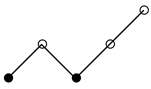
3. Associated Multiple Integrals and 2-Labeled Posets
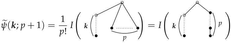
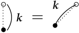
In [37], Yamamoto provided a graphical representation of the iterated integrals of multiple zeta values and their star versions by using 2-posets, which enabled him to discover a few very elegant relations among these values. In this section, we will follow his approach closely and represent M T ¯ Vs using a slightly modified version of these 2-posets. In this way, it is much easier to see many relations between M T ¯ Vs.
Let’s begin by generalizing Yamamoto’s definition of 2-poset so that we can adapt it to the M T ¯ V setting.
Definition 2.
Let κ 0 be a real number and let X = ( X , ) be any partially ordered finite set. Let δ X : X { 0 , κ } be a label map. We then say the pair ( X , δ X ) is a 2-poset targeting at { 0 , κ } . We often call X itself a 2-poset if no confusion arises.
A 2-poset ( X , δ X ) is called admissible if δ X ( x ) = 0 for all maximal elements x ( X , ) and δ X ( x ) = κ for all minimal elements x ( X , ) .
Definition 3.
Let X be an admissible 2-poset X targeting at { 0 , 1 } and set Δ X = ( t x ) x [ 0 , 1 ] X | t x < t y if x < y . We define the (multiple) integral associated with X by
I ( X ) = Δ X x X ω δ X ( x ) ( t x ) ,
where
ω 0 ( t ) = d t t , ω 1 ( t ) = 2 d t 1 + t 2 .
We put I ( ) : = 1 for the empty 2-poset ∅.
Proposition 3.
For non-comparable elements a and b of a 2-poset X, X a b denotes the 2-poset that is obtained from X by adjoining the relation a < b . If X is an admissible 2-poset, then the 2-poset X a b and X b a are admissible and
I ( X ) = I ( X a b ) + I ( X b a ) .
Proof. 
This is clear from the definition. □
Note that the admissibility of a 2-poset corresponds to the convergence of the associated integrals. In what follows, we adopt the usual Hasse diagrams to indicate 2-posets, with vertices ∘ and • corresponding to δ ( x ) = 0 and δ ( x ) = 1 , respectively. For example, the diagram
Mathematics 12 03771 i001
represents the admissible 2-poset X = { x 1 , x 2 , x 3 , x 4 , x 5 } , with the order x 1 < x 2 > x 3 < x 4 < x 5 and label ( δ X ( x 1 ) , , δ X ( x 5 ) ) = ( 1 , 0 , 1 , 0 , 0 ) . To save space, for a composition k = ( k 1 , , k r ) of positive integers, we write Mathematics 12 03771 i002 for the diagrams
Mathematics 12 03771 i003
By the definition of the multiple T ¯ -values, we have
T ¯ ( k ) = ( 1 ) r 0 1 2 d t 1 + t 2 d t t k 1 1 2 d t 1 + t 2 d t t k r 1 .
Hence, using this notation of associated integrals, we can verify that
Mathematics 12 03771 i004
Thus, we may deduce from (4) that
Mathematics 12 03771 i005
since there are exactly p ! ways to impose a total order on the p black vertices. By Proposition 3, this implies that ψ ˜ ( k 1 , , k r ; p + 1 ) can be expressed as a finite sum of M T ¯ Vs. For example, using the shuffle relations of iterated integral (5), we have
B ( 1 ; z ) B ( k 1 , , k r ; z ) = 0 z 2 d t 1 + t 2 0 z 2 d t 1 + t 2 d t t k 1 1 2 d t 1 + t 2 d t t k r 1 = B ( 1 , k 1 , , k r ; z ) + l = 1 r i + j = k l 1 , i , j 0 B ( k 1 , , k l 1 , i + 1 , j + 1 , k l + 1 , , k r 1 , k r ; z ) .
Hence, for p = 1 , we obtain
ψ ˜ ( k ; 2 ) = 0 1 B ( 1 ; z ) B ( k 1 , , k r ; z ) z d z = ( 1 ) r + 1 T ¯ ( 1 , k 1 , , k r 1 , k r + 1 ) + ( 1 ) r + 1 i + j = k r 1 , i , j 0 T ¯ ( k 1 , , k r 1 , i + 1 , j + 2 ) + ( 1 ) r + 1 l = 1 r 1 i + j = k l 1 , i , j 0 T ¯ ( k 1 , , k l 1 , i + 1 , j + 1 , k l + 1 , , k r 1 , k r + 1 ) .
On the other hand, letting p = q = 1 and k r k r + 1 in (23), one obtains
ψ ˜ ( k ; 2 ) = ( 1 ) r π 2 T ¯ ( k 1 , , k r 1 , k r + 1 ) + ( 1 ) r T ¯ ( k 1 , , k r 1 , k r + 1 , 1 ) .
Comparing (27) and (28), we find the following identity of alternating multiple T-values
π 2 T ¯ ( k 1 , , k r 1 , k r + 1 ) + T ¯ ( k 1 , , k r 1 , k r + 1 , 1 ) + T ¯ ( 1 , k 1 , , k r 1 , k r + 1 ) + l = 1 r i + j = k l 1 , i , j 0 T ¯ ( k 1 , , k l 1 , i + 1 , j + 1 , k l + 1 , , k r 1 , k r + 1 ) = 0 ,
where, if l = r , then no component appears after j + 1 in the last sum above.

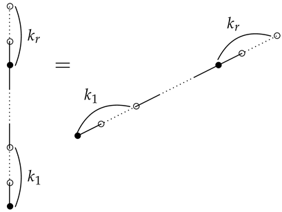
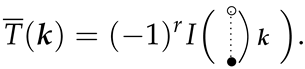
4. Concluding Remarks

We have studied the special values of the Kaneko–Tsumura ψ -functions and its closely related cousin—the Kaneko–Tsumura ψ ˜ -functions—in this paper. By using the method of iterated integrals first developed by K.T. Chen in 1960s and Yamamoto’s recently discovered graphical representation, we have found some nontrivial relations between these values and M T ¯ Vs. As corollaries, we can then discover a few intricate relations among M T ¯ Vs themselves. Previously, we studied the sum formula or the duality formula among Kaneko–Tsumura ψ -values in [9,32]. One may wonder if there are some forms of the sum formula or the duality formula among Kaneko–Tsumura ψ ˜ -values themselves, or similar formulas for M T ¯ Vs themselves. We hope to return to these problems in the future.

Author Contributions

All authors contribute to this work equally. All authors have read and agreed to the published version of the manuscript.

Funding

Ce Xu is supported by the National Natural Science Foundation of China (Grant No. 12101008), the Natural Science Foundation of Anhui Province (Grant No. 2108085QA01), and the University Natural Science Research Project of Anhui Province (Grant No. KJ2020A0057). Jianqiang Zhao is supported by the Jacobs Prize from The Bishop’s School.

Data Availability Statement

We do not have data associated with this paper.

Conflicts of Interest

The authors declare no conflicts of interest.

References

  1. Hoffman, M.E. Multiple harmonic series. Pac. J. Math. 1992, 152, 275–290. [Google Scholar] [CrossRef]
  2. Zagier, D. Values of zeta functions and their applications. In First European Congress of Mathematics; Joseph, A., Mignot, F., Murat, F., Prum, B., Rentschler, R., Eds.; Birkhauser: Basel, Switzerland; Boston, MA, USA; Berlin, Germany, 1994; Volume II, pp. 497–512. [Google Scholar]
  3. Broadhurst, D.J. Conjectured enumeration of irreducible multiple zeta values, from knots and Feynman diagrams. arXiv 1996, arXiv:hep-th/9612012. [Google Scholar]
  4. Broadhurst, D.J. Massive 3-loop Feynman diagrams reducible to SC* primitives of algebras of the sixth root of unity. Eur. Phys. J. C (Fields) 1999, 8, 311–333. [Google Scholar] [CrossRef]
  5. Brown, F. Mixed Tate motives over Z . Ann. Math. 2012, 175, 949–976. [Google Scholar] [CrossRef]
  6. Zudilin, W. Multiple q-zeta brackets. Mathematics 2015, 3, 119–130. [Google Scholar] [CrossRef]
  7. Hoffman, M.E. An odd variant of multiple zeta values. Comm. Number Theory Phys. 2019, 13, 529–567. [Google Scholar] [CrossRef]
  8. Kaneko, M.; Tsumura, H. On multiple zeta values of level two. Tsukuba J. Math. 2020, 44, 213–234. [Google Scholar] [CrossRef]
  9. Xu, C.; Zhao, J. Variants of multiple zeta values with even and odd summation indices. Math. Zeit. 2022, 300, 3109–3142. [Google Scholar] [CrossRef]
  10. Arakawa, T.; Kaneko, M. Multiple zeta values, poly-Bernoulli numbers, and related zeta functions. Nagoya Math. J. 1999, 153, 189–209. [Google Scholar] [CrossRef]
  11. Kaneko, M.; Tsumura, H. Multi-poly-Bernoulli numbers and related zeta functions. Nagoya Math. J. 2018, 232, 19–54. [Google Scholar] [CrossRef]
  12. Hoshi, T. On values of zeta functions of Arakawa–Kaneko type. Comment. Math. Univ. Sancti Pauli 2021, 69, 1–22. [Google Scholar]
  13. Nishibiro, K. On generalization of duality formulas for the Arakawa-Kaneko type zeta functions. arXiv 2023, arXiv:2310.07318. [Google Scholar]
  14. Nishibiro, K. On explicit relations for values of Kaneko–Tsumura’s λ function. Tokyo J. Math. 2024. [Google Scholar] [CrossRef]
  15. Umezawa, R. Multiple T-values and iterated log-tangent integrals. arXiv 2023, arXiv:2301.06067. [Google Scholar]
  16. Euler, L. Meditationes circa singulare serierum genus. Novi Comment. Acad. Sci. Petropolitanae 1776, 20, 140–186. [Google Scholar]
  17. Kaneko, M.; Pallewatta, M.; Tsumura, H. On poly-cosecant numbers. J. Integer Seq. 2020, 23, 20.6.4. [Google Scholar]
  18. Bényi, B.; Josuat-Vergès, M. Combinatorial proof of an identity on Genocchi numbers. J. Integer Seq. 2021, 24, 21.7.6. [Google Scholar]
  19. Bényi, B.; Matsusaka, T. Remarkable relations between the central binomial series, Eulerian polynomials, and poly-Bernoulli numbers. Kyushu J. Math. 2023, 77, 149–158. [Google Scholar] [CrossRef]
  20. Nishibiro, K. On some properties of polycosecant numbers and polycotangent numbers. arXiv 2022, arXiv:2205.05247. [Google Scholar]
  21. Khera, J.; Lundberg, E. The distribution of the length of the longest path in random acyclic orientations of a complete bipartite graph. arXiv 2024, arXiv:2408.12716. [Google Scholar]
  22. Cameron, P.J.; Glass, C.A.; Rekvényi, K.; Schumacher, R.U. Acyclic orientations and poly-Bernoulli numbers. arXiv 2014, arXiv:1412.3685. [Google Scholar]
  23. Kaneko, M.; Ohno, Y. On a kind of duality of multiple zeta-star values. Int. J. Number Theory 2010, 8, 1927–1932. [Google Scholar] [CrossRef]
  24. Si, X.; Luo, F. Another proof of Kaneko–Ohno’s duality formula for multiple zeta star values. In Colloquium Mathematicum; Instytut Matematyczny Polskiej Akademii Nauk: Warsaw, Poland, 2023; Volume 174, pp. 1–11. [Google Scholar]
  25. Kawasaki, N.; Ohno, Y. Combinatorial proofs of identities for special values of Arakawa–Kaneko multiple zeta functions. Kyushu J. Math. 2018, 72, 215–222. [Google Scholar] [CrossRef]
  26. Yamamoto, S. Multiple zeta functions of Kaneko–Tsumura type and their values at positive integers. Kyushu J. Math. 2022, 76, 497–509. [Google Scholar] [CrossRef]
  27. Xu, C. Duality formulas for Arakawa–Kaneko zeta values and related variants. Bull. Malays. Math. Sci. Soc. 2021, 44, 3001–3018. [Google Scholar] [CrossRef]
  28. Luo, F.; Si, X. A note on Arakawa–Kaneko zeta values and Kaneko–Tsumura η-values. Bull. Malays. Math. Sci. Soc. 2023, 46, 21. [Google Scholar] [CrossRef]
  29. Kaneko, M.; Tsumura, H. Zeta functions connecting multiple zeta values and poly-Bernoulli numbers. Adv. Stud. Pure Math. 2020, 84, 181–204. [Google Scholar]
  30. Kaneko, M.; Wang, W.; Xu, C.; Zhao, J. Parametric Apéry-type series and Hurwitz-type multiple zeta values. arXiv 2022, arXiv:2209.06770. [Google Scholar]
  31. Pallewattaa, M.; Xu, C. Some results on Arakawa–Kaneko, Kaneko–Tsumura functions and related functions. Period. Math. Hung. 2024, 89, 175–200. [Google Scholar] [CrossRef]
  32. Xu, C.; Zhao, J. Alternating Multiple T-values: Weighted sums, duality, and dimension Conjecture. Ramanujan J. 2024, 63, 13–54. [Google Scholar] [CrossRef]
  33. Zheng, W.; Yang, Y. Parametric Arakawa–Kaneko zeta function and Kaneko–Tsumura η-function. Bull. Belg. Math. Soc. Simon Stevin 2023, 30, 328–340. [Google Scholar] [CrossRef]
  34. Chen, K.-T. Iterated path integrals. Bull. Am. Math. Soc. 1977, 83, 831–879. [Google Scholar] [CrossRef]
  35. Chen, K.-T. Algebras of iterated path integrals and fundamental groups. Trans. Am. Math. Soc. 1971, 156, 359–379. [Google Scholar] [CrossRef]
  36. Kaneko, M.; Tsumura, H. Multiple L-values of level four, poly-Euler numbers, and related zeta functions. Tohoku Math. J. 2024, 76, 361–389. [Google Scholar] [CrossRef]
  37. Yamamoto, S. Multiple zeta-star values and multiple integrals. RIMS Kôkyûroku Bessatsu 2017, B68, 3–14. [Google Scholar]
Disclaimer/Publisher’s Note: The statements, opinions and data contained in all publications are solely those of the individual author(s) and contributor(s) and not of MDPI and/or the editor(s). MDPI and/or the editor(s) disclaim responsibility for any injury to people or property resulting from any ideas, methods, instructions or products referred to in the content.

