Improved Quantization Method of Coupled Circuits in Charge Discrete Space

Abstract

A quantum theory of mesoscopic circuits, based on the discreteness of electric charges, was recently proposed. However, it is not applied widely, mainly because of the difficulty of the mathematical solution to the finite-difference Schrödinger equation. In this paper, we propose an improved perturbation method to calculate Schrödinger equations of the inductance and capacity coupling mesoscopic circuit. With a unitary transformation, the finite differential Schrödinger equation of the system is divided into two equations in generalized momentum representation. The concrete value of the parameter in circuits is important to solving the equation. Both the perturbation method suitable case and the improved perturbation method suitable case, the wave functions, and energy level of the system are achieved. As an application, the current fluctuations are calculated and discussed. The improved mathematical method would be helpful for the popularization of the quantum circuits theory.

1. Introduction

With the rapid development in nanotechnology and nanoelectronics, the integrated circuits and components have been miniaturized toward a mesoscopic scale [1], therefore, the quantum effects of circuits and components have attracted great interest. In the early 1970s, the LC design circuit was first quantized by comparing it with the quantization process of a harmonic oscillator by Louisell [2]. Then, some complicated circuits were studied, such as the RLC circuit with power [3], coupling circuits [4], and nonlinear circuits [5]. The quantization methods had also made much progress; the path integral method [6], canonical transformation method [7] and quantum invariant method [8] were involved in quantizing mesoscopic circuits. Significant progress appeared in 1996, when an advanced quantization method was proposed by Youquan Li [9], which firstly considered the discreteness of electronic charge on the Capacitor plate, and caused a new research hotspot in the quantum circuits theory [10,11,12,13,14,15,16,17]. However, in the framework of advanced quantum theory, the quantization of the circuits and mathematical solution of finite-difference Schrödinger equation are very complicated, which is the main difficulty in applying the theory.

During the last 30 years, quantum optics has made significant progress in both theoretical and experimental research [18,19,20]. Quantum superconducting circuits, as an experimental platform for realizing the interaction between quantum optical fields and artificial atoms, are considered promising candidates for future quantum computing due to their easy integration with existing integrated circuits [21]. Stimulated by the quest to build superconducting quantum processors, a theory of circuit quantum electrodynamics (circuit QED) has emerged [18,21]. In complex quantum superconducting circuits, the basic unit in systems such as coupling devices, read-out systems, and transmission lines is the LC resonant circuit. Faced with increasingly complex quantum superconducting circuits and coupling strength, higher requirements have been put forward for the basic research work of LC resonant circuits [22].

In this paper, the inductance and capacity of the coupling mesoscopic circuit is studied in the framework of advanced quantum theory. With a unitary transformation, the finite differential Schrödinger equation of the system would be divided into two equations in generalized momentum representation. Solving the equation is dependent on the concrete value of the parameter in circuits. Firstly, the equations are resolved with the perturbation method suitable case. Then, we propose an improved perturbation method in case of parameter $\xi$ not being small enough. As an application, the wave functions, energy level, and current fluctuations of the system are all calculated and compared in both cases. The improved mathematical method would be helpful to the popularization of quantum circuits theory.

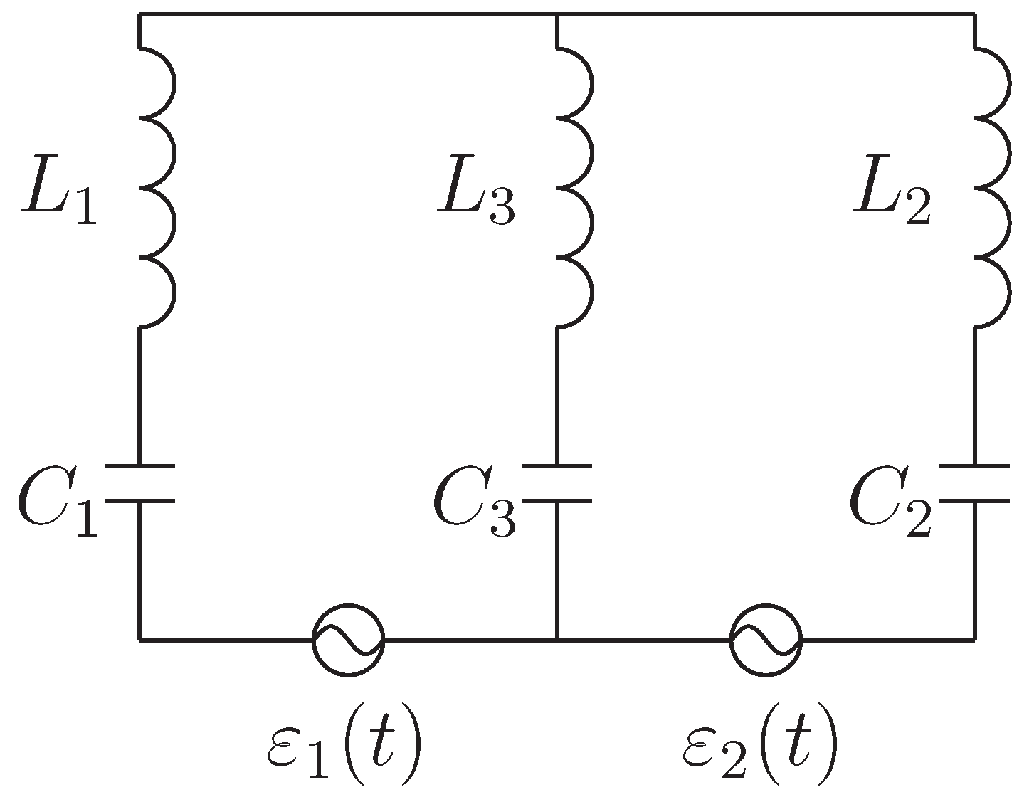
2. Schrödinger Equation of the System

Two LC circuits coupled via inductance and capacitance, with the source in each of the circuits, are sketched in Figure 1.

In which, $L_i$ and $C_i(i=1,2)$ are the inductance and capacitance of each component circuit, respectively. $L_3$ and $C_3$ are the coupling inductance and capacitance between two circuits. ${ϵ}_i(i=1,2)$ are the driving sources in the branch of the coupling system.

According to the advanced quantum theory for mesoscopic electric circuits [9], $\widehat{q}$ takes discrete values

$$\widehat{q}|n>=n{q}_e|n>.$$

(1)

With the minimum ‘shift operator’, which is defined as

$$\widehat{Q}=e^{i{q}_e\widehat{p}/\hslash }.$$

(2)

The Schrödinger equation of the mesoscopic inductive and capacitive coupling circuits is written as

$$\begin{array}{ccc}\hfill \{& -& {\displaystyle \frac{{\hslash }^2}{2L_1{q}_e}}({\nabla }_{q_e}^{\left(1\right)}-{\overline{\nabla }}_{q_e}^{\left(1\right)})-{\displaystyle \frac{{\hslash }^2}{2L_2{q}_e}}({\nabla }_{q_e}^{\left(2\right)}-{\overline{\nabla }}_{q_e}^{\left(2\right)})\hfill \\ & -& {\displaystyle \frac{{\hslash }^2}{8}}{L}_3{\left[{\displaystyle \frac{1}{L_1}}({\nabla }_{q_e}^{\left(1\right)}+{\overline{\nabla }}_{q_e}^{\left(1\right)})-{\displaystyle \frac{1}{L_2}}({\nabla }_{q_e}^{\left(2\right)}+{\overline{\nabla }}_{q_e}^{\left(2\right)})\right]}^2\hfill \\ & +& {\displaystyle \frac{{\widehat{q}}_1^2}{2C_1}}+{\displaystyle \frac{{\widehat{q}}_2^2}{2C_2}}+{\displaystyle \frac{{({\widehat{q}}_1-{\widehat{q}}_2)}^2}{2C_3}}-{\widehat{q}}_1{\epsilon }_1-{\widehat{q}}_2{\epsilon }_2\left\}\right|\psi >=E|\psi >.\hfill \end{array}$$

(3)

In above, the right and left discrete derivative operators are

$${\nabla }_{q_e}=(\widehat{Q}-1)/q_e,{\overline{\nabla }}_{q_e}=(1-{\widehat{Q}}^{+})/q_e.$$

(4)

With an appropriate unitary transformation and choosing appropriate values of $L_i$, $C_i$ (see the discussion on Figure 2 and [15]), the finite differential Schrödinger Equation (3) of the system would be divided into two equations in generalized momentum representation. We must demonstrate how to choose $L_i$ and $C_i$.

$$\left\{-{\displaystyle \frac{{\hslash }^2{\beta }_1}{2}}{\displaystyle \frac{{\partial }^2}{\partial {p^{\prime }}_1^2}}-{\displaystyle \frac{{\hslash }^2}{q_e^2{\alpha }_1}}\left[cos\left({\displaystyle \frac{q_e}{\hslash }}{\gamma }_1{p^{\prime }}_1\right)-1\right]\right\}\psi \left(p_1^{\prime }\right)=E^{\left(1\right)}\psi \left(p_1^{\prime }\right),$$

(5)

$$\left\{-{\displaystyle \frac{{\hslash }^2{\beta }_2}{2}}{\displaystyle \frac{{\partial }^2}{\partial {p^{\prime }}_2^2}}-{\displaystyle \frac{{\hslash }^2}{q_e^2{\alpha }_2}}\left[cos\left({\displaystyle \frac{q_e}{\hslash }}{\gamma }_2{p^{\prime }}_2\right)-1\right]\right\}\psi \left(p_2^{\prime }\right)=E^{\left(2\right)}\psi \left(p_2^{\prime }\right)$$

(6)

where, $p_i(i=1,2)$ is the ’generalized momentum’ conjugate with ’generalized coordinates’ $q_i\left(t\right)$. and ${\alpha }_i$, ${\beta }_i$, ${\gamma }_i(i=1,2)$ are related to the parameters $L_i$, $C_i$ and ${\epsilon }_i(i=1,2)$ in the circuits. For detailed derivation, see Appendix A.

By introducing

$$\begin{array}{c}\hfill z_i={\displaystyle \frac{\pi }{2}}-{\displaystyle \frac{q_e{\gamma }_i}{2\hslash }}{p}_i^{\prime },\\ \hfill {\lambda }^{\left(i\right)}={\displaystyle \frac{8E^{\left(i\right)}}{{\beta }_i{q}_e^2{\gamma }_i^2}}-{\displaystyle \frac{8{\hslash }^2}{{\beta }_i{q}_e^4{\gamma }_i^2{\alpha }_i}},\\ \hfill {\xi }_i=-{\displaystyle \frac{4{\hslash }^2}{{\beta }_i{q}_e^4{\gamma }_i^2{\alpha }_i}}\end{array}$$

(7)

in which $i=1,2$. The Schrödinger equation is converted to a standard Mathieu equation,

$$\left[{\displaystyle \frac{{\partial }^2}{\partial z_i^2}}+\left({\lambda }^{\left(i\right)}+2{\xi }_{i}cos2z_i\right)\right]\psi \left(z_i\right)=0.$$

(8)

In terms of the conventional notations, the solutions are ${\psi }_l^{+}=c{e}_l(z,\xi )$, ${\psi }_l^{-}=s{e}_{l+1}(z,\xi )$ in the case of $\xi$ is small [12,23]. However, it is a rather complicated method, and cannot be applied to all kinds of circuits. In a previous paper, we proposed a perturbation method based on series expansion to resolve the equation [14], especially, since it is an applicative method to resolve higher-order difference equations.

Now, let us first discuss how $sin(\theta /2)$ and ${\xi }_i$ are affected by $L_i$ and $C_i$. In the quantum circuit experiments [21,24], the value range of $L_i$ is ${10}^{-9}\sim {10}^{-6}H$, and the value range of $C_i$ is ${10}^{-12}\sim {10}^{-15}F$. According to the numerator of Equation (A7), $L_i$ and $C_i$ should meet the conditions $L_1·C_1\ge L_3·C_3$ and $L_2·C_2\ge L_3·C_3$.

In Figure 2, using the coupling inductance $L_3$ as a variable, we calculated $sin(\theta /2)$ and ${\xi }_{1,2}$, with $L_{1,2}={10}^{-6}H$, $C_{1,3}={10}^{-15}F$, $C_2={10}^{-12}F$. As shown by the blue-dot line in Figure 2, it can satisfy the approximate conditions for deriving Equations (5) and (6). Similarly, the black solid line shows that as $L_3$ in the range of ${10}^{-9}$ to ${10}^{-6}$, ${\xi }_1$ remains less than 0.03, especially when $L_3\sim {10}^{-6}$, ${\xi }_1$ tends to 0. This provides a good approximation condition for solving the Mathieu Equation (8) using the perturbation method. However, as $L_3$ approaches ${10}^{-6}$ from ${10}^{-9}$, ${\xi }_2$ gradually moves away from 0, as seen by the red-dash line. When $L_3$ tends to ${10}^{-6}$, ${\xi }_2$ is much greater than 1, so ${\xi }_2$ is not suitable as a perturbation parameter in this case, and it is necessary to find a new parameter.

3. Resolution of the Schrödinger Equation: Perturbation Method Suitable Case (PMSC)

Sine Equations (5) and (6) are alike, we drop off the superscript and subscript i in the following text for convenience.

If $\xi$ is a small parameter, it is a perturbation method suitable case (PMSC). $\psi \left(z\right)$ could be a periodic function of $\pi$ or $2\pi$. We show the calculation process of $\psi \left(z\right)$ with the periodic $\pi$, let

$$\psi \left(z\right)=b_0+\sum _{k=2,4,6\dots }^{\infty }(a_{k}sinkz+b_{k}coskz).$$

(9)

By inserting Equation (9) into Equation (8), calculating to the order k = 8, we obtain

$$\begin{array}{ccc}& & \lambda d_0-\xi d_2\hfill \\ & +& (-4a_2+\lambda a_2-\xi a_4)sin2z\hfill \\ & +& (-2\xi b_0-4b_2+\lambda b_2-\xi b_4)cos2z\hfill \\ & +& (-\xi a_2-16a_4+\lambda a_4-\xi a_6)sin4z\hfill \\ & +& (-\xi b_2-16b_4+\lambda b_4-\xi b_6)cos4z\hfill \\ & +& (-\xi a_4-36a_6+\lambda a_6-\xi a_8)sin6z\hfill \\ & +& (-\xi b_4-36b_6+\lambda b_6-\xi b_8)cos6z\hfill \\ & +& (-\xi a_6-64a_8+\lambda a_8)sin8z\hfill \\ & +& (-\xi b_6-64b_8+\lambda d_8)cos8z\hfill \\ & +& \dots =0.\hfill \end{array}$$

(10)

Obviously, the coefficients satisfy the following matrix equation

$$\left(\begin{array}{ccccc}\lambda & \xi & 0& 0& \dots \\ \xi & -4+\lambda & \xi & 0& \dots \\ 0& \xi & -16+\lambda & \xi & \dots \\ 0& 0& \xi & -36+\lambda & \dots \\ 0& 0& 0& \xi & \dots \\ \dots & \dots & \dots & \dots & \dots \end{array}\right)·\left(\begin{array}{c}{a}_2\\ a_4\\ a_6\\ a_8\\ \dots \end{array}\right)=0,$$

(11)

$$\left(\begin{array}{cccccc}\lambda & \xi & 0& 0& 0& \dots \\ \xi & -4+\lambda & \xi & 0& 0& \dots \\ 0& \xi & -16+\lambda & \xi & 0& \dots \\ 0& 0& \xi & -36+\lambda & \xi & \dots \\ 0& 0& 0& \xi & -64+\lambda & \dots \\ 0& 0& 0& 0& \xi & \dots \\ \dots & \dots & \dots & \dots & \dots & \dots \end{array}\right)·\left(\begin{array}{c}{b}_0\\ b_2\\ b_4\\ b_6\\ b_8\\ \dots \end{array}\right)=0.$$

(12)

If $\xi$ is small, perturbation theory is valid. The zero-order approximate of $\lambda$ is easily obtained from the diagonal elements of the coefficients matrix,

$$\lambda =k^4,k=0,1,2,3\cdots .$$

(13)

The eigenvalue $\lambda$ and eigenstate $\psi$ can be expressed with $\xi$ as

$$\lambda ={\lambda }_0+{\lambda }_1\xi +{\lambda }_2{\xi }^2+{\lambda }_3{\xi }^3+\cdots ,$$

$$\psi ={\psi }_0+\xi {\psi }_1+{\xi }^2{\psi }_2+{\xi }^3{\psi }_3+\cdots$$

(14)

where ${\psi }_0$ and ${\lambda }_0=k^2$ are zero-order approximate of wave function and eigenvalue, ${\psi }_1$, ${\psi }_2$, ${\psi }_3$ and ${\lambda }_1$, ${\lambda }_2$, ${\lambda }_3$ are high order corrections of them. Calculated to second order approximate, they are determined by the following equations,

$${\psi }_0^{″}+{\lambda }_0{\psi }_0=0,$$

$${\psi }_1^{″}+{\lambda }_0{\psi }_1=-{\lambda }_1{\psi }_0-2{\psi }_{0}cos2z,$$

$${\psi }_2^{″}+{\lambda }_0{\psi }_2=-{\lambda }_1{\psi }_1-{\lambda }_2{\psi }_0-2{\psi }_{1}cos2z,$$

$$\dots$$

(15)

Then, high order approximates of ${\lambda }_k$ and ${\psi }_k$ could be calculated. We calculate $\lambda$ and $\psi$ as an example when $k=0$, ${\lambda }_0=0$.

The zero-order approximated solution of ${\psi }_0$ could obtained from the first formula of Equation (15)

$${\psi }_0=c$$

(16)

inserting ${\psi }_0$ into the second formula of Equation (15), it reads as

$${\psi }_1^{″}=-{\lambda }_{1}c-2ccos2z$$

in the equation above, let ${\lambda }_1=0$, ${\psi }_1$ have a period solution, satisfied:

$${\psi }_1^{″}=-2ccos2z$$

the solution of ${\psi }_1$ is

$${\psi }_1={\displaystyle \frac{c}{2}}cos2z$$

(17)

insert ${\psi }_0$, ${\psi }_1$ into the third formula of Equation (15),

$${\psi }_2^{″}=-{\lambda }_{2}c-{\displaystyle \frac{c}{2}}-{\displaystyle \frac{c}{2}}cos4z$$

let ${\lambda }_2=-{\displaystyle \frac{1}{2}}$, ${\psi }_2$ have a period solution.

When $k=0$, the final results of $\psi$ and $\lambda$ are

$$\sqrt{2}{\psi }_{k=0}=1+{\displaystyle \frac{2{\hslash }^2}{{\beta }_1{q}_e^4{\gamma }_1^2{\alpha }_1}}cos{\displaystyle \frac{q_e{\gamma }_1}{\hslash }}{p}_1^{\prime }+\dots ,$$

(18)

$$\lambda =-{\displaystyle \frac{1}{2}}{\xi }^2+O\left({\xi }^3\right).$$

(19)

For normalization, $c={\displaystyle \frac{1}{\sqrt{2}}}$ in $\psi$. The correspondent energy is derived from Equation (19)

$$E_{k=0}={\displaystyle \frac{{\hslash }^2}{q_e^2{\alpha }_1}}-{\beta }_1{q}_e^2{\gamma }_1^2{\left({\displaystyle \frac{{\hslash }^2}{{\beta }_1{q}_e^4{\gamma }_1^2{\alpha }_1}}\right)}^2+O\left({\xi }^3\right).$$

(20)

The other wave function and energy level can be obtained with similar calculation processes.

$${\psi }_1^{-}=sin{\displaystyle \frac{q_e{\gamma }_1}{\hslash }}{p}_1^{\prime }+{\displaystyle \frac{{\hslash }^2}{2{\beta }_1{q}_e^4{\gamma }_1^2{\alpha }_1}}sin{\displaystyle \frac{3q_e{\gamma }_1}{2\hslash }}{p}_1^{\prime }+\dots ,$$

$${\psi }_1^{+}=cos{\displaystyle \frac{q_e{\gamma }_1}{2\hslash }}{p}_1^{\prime }+{\displaystyle \frac{{\hslash }^2}{2{\beta }_1{q}_e^4{\gamma }_1^2{\alpha }_1}}cos{\displaystyle \frac{3q_e{\gamma }_1}{2\hslash }}{p}^{\prime }+\dots ,$$

$${\psi }_2^{-}=cos{\displaystyle \frac{q_e{\gamma }_1}{\hslash }}{p}_1^{\prime }+{\displaystyle \frac{{\hslash }^2}{{\beta }_1{q}_e^4{\gamma }_1^2{\alpha }_1}}\left({\displaystyle \frac{1}{3}}cos{\displaystyle \frac{4q_e{\gamma }_1}{\sqrt{2}\hslash }}{p^{\prime }}_1-1\right)+\dots ,$$

$${\psi }_2^{+}=sin{\displaystyle \frac{q_e{\gamma }_1}{\hslash }}{p}_1^{\prime }+{\displaystyle \frac{{\hslash }^2}{2{\beta }_1{q}_e^4{\gamma }_1^2{\alpha }_1}}\left({\displaystyle \frac{1}{3}}sin{\displaystyle \frac{4q_e{\gamma }_1}{\sqrt{2}\hslash }}{p^{\prime }}_1+1\right)+\dots$$

(21)

while the superscripts ‘+’ and ‘-’ specify the even and odd parity solution respectively. The results are consistent with the expression of $c{e}_l$ and $s{e}_{l+1}$.

The corresponding energy levels are

$$E_1^{-}={\displaystyle \frac{3{\hslash }^2}{2q_e^2{\alpha }_1}}+{\displaystyle \frac{{\beta }_1{q}_e^2{\gamma }_1^2}{8}}-{\displaystyle \frac{{\beta }_1{q}_e^2{\gamma }_1^2}{4}}{\left({\displaystyle \frac{{\hslash }^2}{{\beta }_1{q}_e^4{\gamma }_1^2{\alpha }_1}}\right)}^2+O\left({\xi }^3\right),$$

$$E_1^{+}={\displaystyle \frac{{\hslash }^2}{2q_e^2{\alpha }_1}}+{\displaystyle \frac{{\beta }_1{q}_e^2{\gamma }_1^2}{8}}-{\displaystyle \frac{{\beta }_1{q}_e^2{\gamma }_1^2}{4}}{\left({\displaystyle \frac{{\hslash }^2}{{\beta }_1{q}_e^4{\gamma }_1^2{\alpha }_1}}\right)}^2+O\left({\xi }^3\right),$$

$$E_2^{-}={\displaystyle \frac{{\hslash }^2}{q_e^2{\alpha }_1}}+{\displaystyle \frac{{\beta }_1{q}_e^2{\gamma }_1^2}{2}}+{\displaystyle \frac{5{\beta }_1{q}_e^2{\gamma }_1^2}{6}}{\left({\displaystyle \frac{{\hslash }^2}{{\beta }_1{q}_e^4{\gamma }_1^2{\alpha }_1}}\right)}^2+O\left({\xi }^3\right),$$

$$E_2^{+}={\displaystyle \frac{{\hslash }^2}{q_e^2{\alpha }_1}}+{\displaystyle \frac{{\beta }_1{q}_e^2{\gamma }_1^2}{2}}-{\displaystyle \frac{{\beta }_1{q}_e^2{\gamma }_1^2}{6}}{\left({\displaystyle \frac{{\hslash }^2}{{\beta }_1{q}_e^4{\gamma }_1^2{\alpha }_1}}\right)}^2+O\left({\xi }^3\right).$$

(22)

In calculation, we found that the energy spectrum $E_k^{+}$ and $E_k^{-}$ would have the same expression when $k\ge 3$. This does not mean the degeneration of energy level because we only calculated to ${\xi }^2$ phase.

4. Resolution of the Schrödinger Equation: Improved Perturbation Method Suitable Case (IPMSC)

In the above, the Schrödinger equation is calculated in the case of $\xi <<1$. However, not all circuits satisfy the particular requirement. Considering the general situation, when $\xi$ is not a small parameter, a new small parameter is needed to satisfy the application of the perturbation method, it is the improved perturbation method suitable case (IPMSC). We introduce a new variable defined as

$$\alpha ={\displaystyle \frac{{\lambda }_1\xi }{1+{\lambda }_1\xi }}.$$

(23)

The eigenvalue $\lambda$ and eigenstate $\psi$ can be expressed with $\alpha$ as

$$\psi ={\psi }_0+\alpha {\psi }_1+{\alpha }^2{\psi }_2+{\alpha }^3{\psi }_3+\cdots ,$$

$$\lambda ={\lambda }_0+({\lambda }_1-2){\lambda }_1^{-1}\alpha +{\lambda }_2{\alpha }^2+\cdots .$$

(24)

Calculated to second order approximate, the corrections to the wave function ${\psi }_1$, ${\psi }_2$, ${\psi }_3$ and eigenvalue ${\lambda }_1$, ${\lambda }_2$, ${\lambda }_3$ are determined by the following equations

$${\psi }_0^{″}+{\lambda }_0{\psi }_0=0,$$

$${\psi }_1^{″}+{\lambda }_0{\psi }_1=-({\lambda }_1-2){\lambda }_1^{-1}{\psi }_0-2{\psi }_0{\lambda }_1^{-1}cos2z,$$

$${\psi }_2^{″}+{\lambda }_0{\psi }_2=-({\lambda }_1-2){\lambda }_1^{-1}{\psi }_1-{\lambda }_2{\psi }_0-2{\lambda }_1^{-1}({\psi }_0+{\psi }_1)cos2z,$$

$$\dots$$

(25)

The wave functions of the system are

$$\sqrt{2}{\psi }_{k=0}=1+{\displaystyle \frac{2{\hslash }^2}{{\beta }_1{q}_e^4{\gamma }_1^2{\alpha }_1-8{\hslash }^2}}cos\left({\displaystyle \frac{q_e{\gamma }_1}{\hslash }}{p}_1^{\prime }\right)+\cdots ,$$

$${\psi }_1^{-}=sin{\displaystyle \frac{q_e{\gamma }_1}{2\hslash }}{p}_1^{\prime }+{\displaystyle \frac{{\hslash }^2}{2({\beta }_1{q}_e^4{\gamma }_1^2{\alpha }_1-4{\hslash }^2)}}sin{\displaystyle \frac{3q_e{\gamma }_1}{\hslash }}{p}_1^{\prime }+\cdots ,$$

$${\psi }_1^{+}=cos{\displaystyle \frac{q_e{\gamma }_1}{\hslash }}{p}_1^{\prime }+{\displaystyle \frac{{\hslash }^2}{2({\beta }_1{q}_e^4{\gamma }_1^2{\alpha }_1-12{\hslash }^2)}}cos{\displaystyle \frac{3q_e{\gamma }_1}{2\hslash }}{p}_1^{\prime }+\cdots ,$$

$${\psi }_2^{-}=cos\left({\displaystyle \frac{q_e{\gamma }_1}{\hslash }}{p}_1^{\prime }\right)-{\displaystyle \frac{{\hslash }^2[1-\frac{1}{3}cos\left(\frac{2q_e{\gamma }_1}{\hslash }{p}_1^{\prime }\right)]}{{\beta }_1{q}_e^4{\gamma }_1^2{\alpha }_1-8{\hslash }^2}}+\cdots ,$$

$${\psi }_2^{+}=sin\left({\displaystyle \frac{q_e{\gamma }_1}{\hslash }}{p}_1^{\prime }\right)-{\displaystyle \frac{{\hslash }^{2}sin\left(\frac{2q_e{\gamma }_1}{\hslash }{p}_1^{\prime }\right)}{3{\beta }_1{q}_e^4{\gamma }_1^2{\alpha }_1-24{\hslash }^2}}+\cdots .$$

(26)

The correspondence energy spectrum are

$$E_{k=0}={\displaystyle \frac{{\hslash }^2}{q_e^2{\alpha }_1}}-{\beta }_1{q}_e^2{\gamma }_1^2{\left[{\displaystyle \frac{{\hslash }^2}{8{\hslash }^2-{\beta }_1{q}_e^4{\gamma }_1^2{\alpha }_1}}\right]}^2+O\left({\alpha }^3\right),$$

$$E_1^{-}={\displaystyle \frac{{\hslash }^2}{q_e^2{\alpha }_1}}+{\displaystyle \frac{{\beta }_1{q}_e^2{\gamma }_1^2}{8}}+{\displaystyle \frac{{\hslash }^2{\beta }_1{q}_e^2{\gamma }_1^2}{2{\beta }_1{q}_e^4{\gamma }_1^2{\alpha }_1-8{\hslash }^2}}-{\displaystyle \frac{9}{4}}{\beta }_1{q}_e^2{\gamma }_1^2$$

$$·{\left({\displaystyle \frac{{\hslash }^2}{{\beta }_1{q}_e^4{\gamma }_1^2{\alpha }_1-4{\hslash }^2}}\right)}^2+O\left({\alpha }^3\right),$$

$$E_1^{+}={\displaystyle \frac{{\hslash }^2}{q_e^2{\alpha }_1}}+{\displaystyle \frac{{\beta }_1{q}_e^2{\gamma }_1^2}{8}}-{\displaystyle \frac{{\beta }_1{q}_e^2{\gamma }_1^2{\hslash }^2}{2{\beta }_1{q}_e^4{\gamma }_1^2{\alpha }_1-24{\hslash }^2}}+{\displaystyle \frac{23{\beta }_1{q}_e^2{\gamma }_1^2}{4}}$$

$$·{\left({\displaystyle \frac{12{\hslash }^2}{{\beta }_1{q}_e^4{\gamma }_1^2{\alpha }_1-12{\hslash }^2}}\right)}^2+O\left({\alpha }^3\right),$$

$$E_2^{-}={\displaystyle \frac{{\hslash }^2}{q_e^2{\alpha }_1}}+{\displaystyle \frac{{\beta }_1{q}_e^2{\gamma }_1^2}{2}}+{\displaystyle \frac{5{\beta }_1{q}_e^2{\gamma }_1^2}{6}}{\left({\displaystyle \frac{{\hslash }^2}{{\beta }_1{q}_e^4{\gamma }_1^2{\alpha }_1-8{\hslash }^2}}\right)}^2+O\left({\alpha }^3\right),$$

$$E_2^{+}={\displaystyle \frac{{\hslash }^2}{q_e^2{\alpha }_1}}+{\displaystyle \frac{{\beta }_1{q}_e^2{\gamma }_1^2}{2}}-{\displaystyle \frac{{\beta }_1{q}_e^2{\gamma }_1^2}{6}}{\left({\displaystyle \frac{{\hslash }^2}{{\beta }_1{q}_e^4{\gamma }_1^2{\alpha }_1-8{\hslash }^2}}\right)}^2+O\left({\alpha }^3\right).$$

(27)

Now, let us verify the above results taking $E_{k=0}$ as an example. Using the definition of $\xi$ by (7), $E_{k=0}$ is rewritten as

$$E_{k=0}={\displaystyle \frac{{\hslash }^2}{q_e^2{\alpha }_1}}-{\displaystyle \frac{{\beta }_1{q}_e^2{\gamma }_1^2}{64}}{\left[{\displaystyle \frac{2\xi }{1+2\xi }}\right]}^2+O\left({\alpha }^3\right).$$

If $\xi <<1$, let ${\displaystyle \frac{2\xi }{1+2\xi }}\approx 2\xi$, then, the above result returns to Equation (20). Similarly, it can be verified that other energy levels in the improved perturbation method suitable case are consistent with the corresponding results in the perturbation method suitable case.

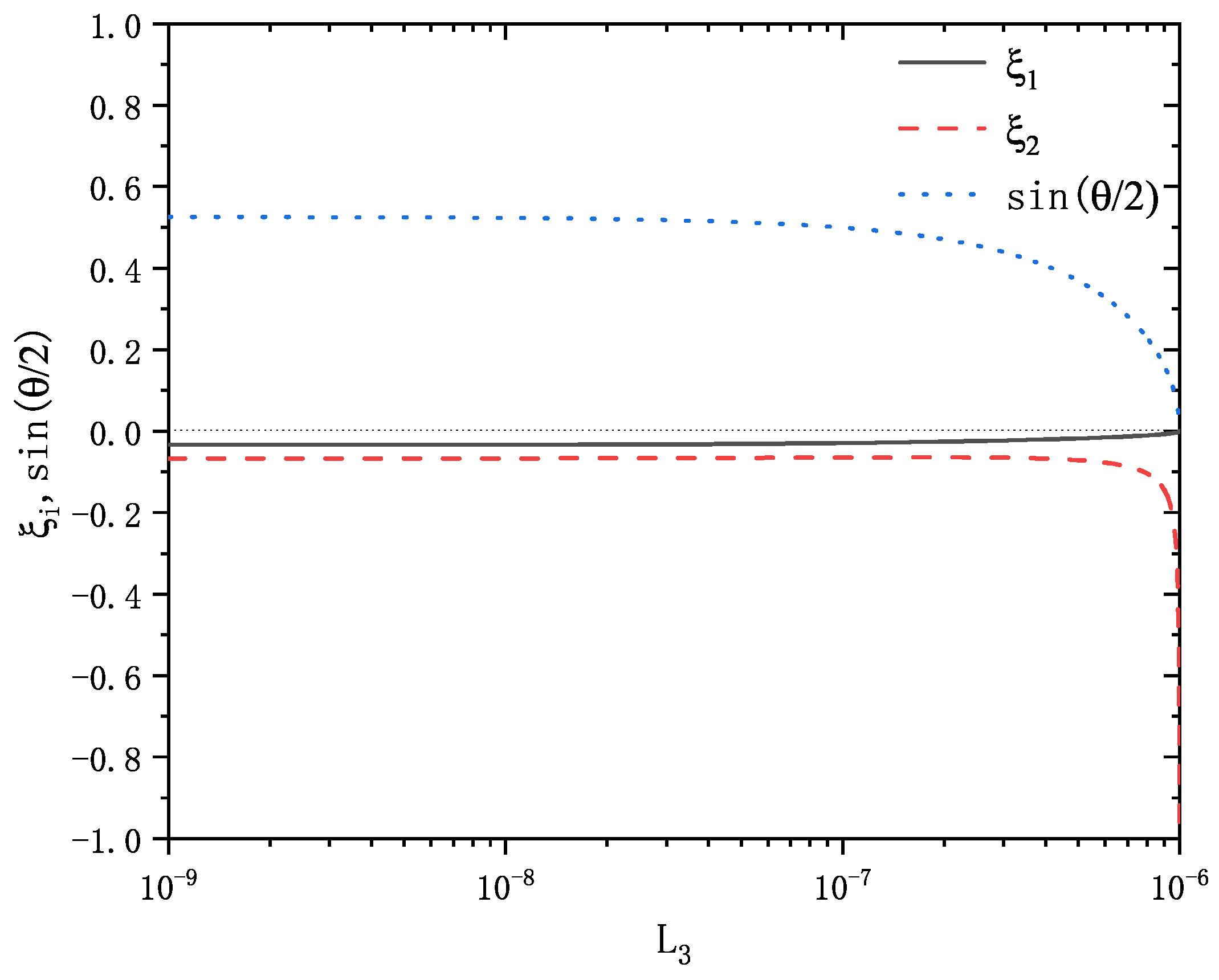
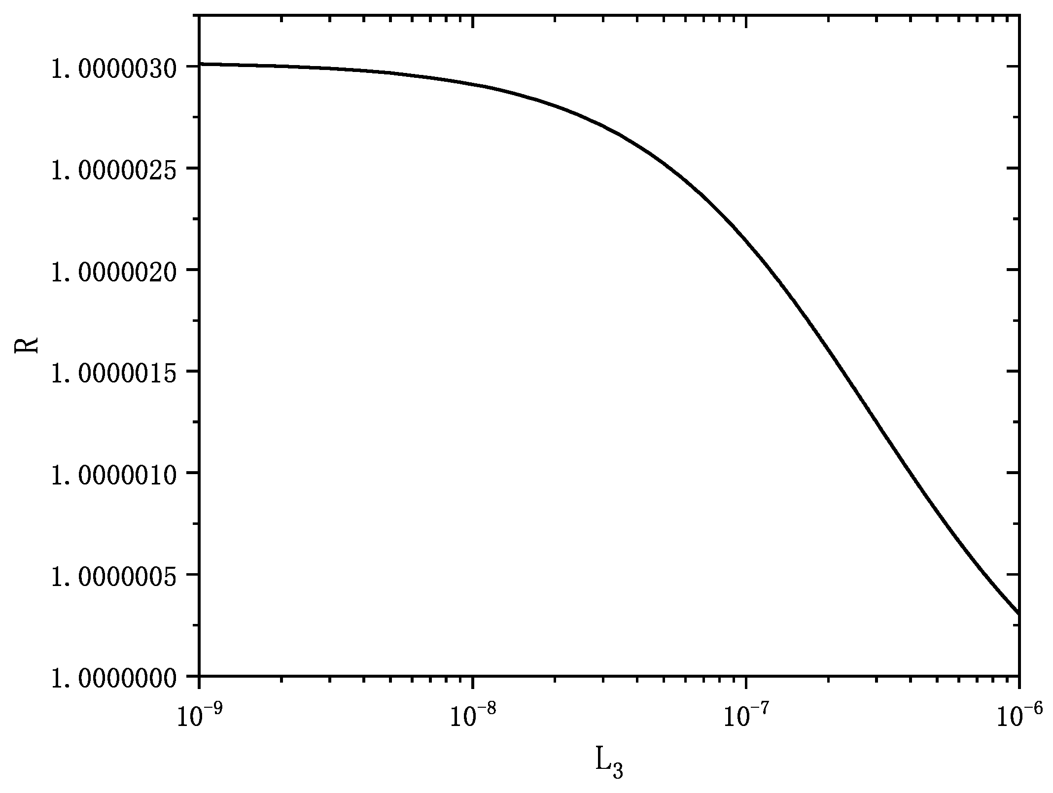
5. Discussion: Quantum Fluctuation in the System

As an application of the results obtained above, we calculated the average values of current $P_1$ and $P_1^2$ in the ground state. In the advanced quantum theory of mesoscopic circuit, the current in the circuit is defined as [9]

$$P_1=-{\displaystyle \frac{\hslash }{2i}}({\nabla }_{q_e}^{\left(1\right)}+{\overline{\nabla }}_{q_e}^{\left(1\right)}).$$

(28)

For perturbation method suitable case,

$$<P{>}_{0\left(PMSC\right)}=0,$$

$$<P_1^2{>}_{0\left(PMSC\right)}={\displaystyle \frac{{\hslash }^2}{4q_e^2}}+{\displaystyle \frac{{\hslash }^6}{4q_e^{10}{\gamma }_1^4{\alpha }_1^2{\beta }_1^2}}+\cdots .$$

(29)

For improved perturbation method suitable case,

$$<P_1{>}_{0\left(IPMSC\right)}=0,$$

$$<P_1^2{>}_{0\left(IPMSC\right)}={\displaystyle \frac{{\hslash }^2}{4q_e^2}}+{\displaystyle \frac{{\hslash }^6}{4q_e^{10}{\gamma }_1^4{\alpha }_1^2{\beta }_1^2}}-{\displaystyle \frac{4{\hslash }^8}{q_e^{14}{\gamma }_1^6{\alpha }_1^3{\beta }_1^3}}$$

$$+{\displaystyle \frac{16{\hslash }^{10}}{q_e^{18}{\gamma }_1^8{\alpha }_1^4{\beta }_1^4}}+\cdots .$$

(30)

From Equations (29) and (30), we can see that the average value of the current in the ground state is zero, whereas the average value of the square of the current is not. This indicates the existence of the current quantum fluctuations, which is the shot noise in the system. The fluctuations between the two circuits are correlated.

To show the difference of $<P_1^2{>}_0$ between the two cases, we calculated the ratio R in the region of ${10}^{-9}H<L_3<{10}^{-6}H$,

$$R={\displaystyle \frac{<P_1^2{>}_{0\left(IPMSC\right)}}{<P_1^2{>}_{0\left(PMSC\right)}}}.$$

In calculation, the concrete values are used: $\hslash =1.05\times {10}^{-34}J·s$, $q_e=1.6\times {10}^{-19}$C, $C_1=1\times {10}^{-15}F$, $C_2=1\times {10}^{-12}F$, $C_3=1\times {10}^{-15}F$, $L_1=1\times {10}^{-6}H$, $L_2=1\times {10}^{-6}H$.

Figure 3 shows that the ratio decreases when the coupling inductance $L_3$ increases, the reason being that the circuit could be regarded as a macroscopic system when $L_3$ is large enough. Furthermore, R is larger than 1, it means the value of $<P_1^2{>}_0$ in IPMSC is bigger than that in PMSC, it indicates a big quantum noise when $\xi$ is a big parameter. The control of $\xi$ would decrease the noise in the circuits system.

6. Conclusions

In the above, the mesoscopic inductance and capacity coupling circuit is quantized in the framework of an advanced quantum theory. With a unitary transformation, the finite-differential Schrödinger equation of the system would be divided into two Mathieu equations in generalized momentum representation. When $\xi$ is a small parameter, the perturbation method could be used to resolve equations; when $\xi$ is not small, a new small parameter is defined to expand the wave function and eigenvalue. In both of the two cases, the wave functions and energy spectrum are achieved. As an application, the current fluctuations are calculated and discussed. The results show that the currents fluctuations of two circuits exist and correlated. A big parameter indicates a big quantum noise in the circuits. An improved perturbation method would be helpful for the popularization of the mesoscopic quantum theory.

References

1. Buot, F.A. Mesoscopic physics and nanoelectronics: Nanoscience and nanotechnology. Phys. Rep. 1993, 234, 73–174. [Google Scholar] [CrossRef]
2. Louisell, W.H. Quantum Statistical Properties of Radiation, 3rd ed.; John Wiley: New York, NY, USA, 1973; pp. 231–235. [Google Scholar]
3. Zhang, Z.M.; He, L.S.; Zhou, S.K. A quantum theory of an RLC circuit with a source. Phys. Lett. A 1998, 244, 196–200. [Google Scholar] [CrossRef]
4. Fan, H.Y.; Pan, X.Y. Quantization and squeezed state of two L-C Circuits with mutual-inductance. Chin. Phys. Lett. 1998, 15, 625–627. [Google Scholar] [CrossRef]
5. Zhang, S.; Um, C.I.; Yeon, K.H. Zero-point energy in a mesoscopic nonlinear inductance-capacitance circuit. Chin. Phys. Lett. 2002, 19, 985–987. [Google Scholar]
6. Yan, Z.Y.; Xu, S.L.; MA, J.Y. Path Integral Solutions of RLC Mesoscopic Circuit with Source. Mod. Phys. Lett. B 2012, 26, 1250058–1250065. [Google Scholar] [CrossRef]
7. Fan, H.Y.; Liang, X.T. Quantum Fluctuation in Thermal Vacuum State for Mesoscopic LC Electric Circuit. Chin. Phys. Lett. 2000, 17, 174–176. [Google Scholar] [CrossRef]
8. Pedrosa, I.A. Quantum description of a time-dependent mesoscopic RLC circuit. Phys. Scr. 2012, T151, 014042–014044. [Google Scholar] [CrossRef]
9. Li, Y.Q.; Chen, B. Quantum theory for mesoscopic electric circuits. Phys. Rev. B 1996, 53, 4027–4032. [Google Scholar] [CrossRef]
10. Flores, J.C. Mesoscopic circuits with charge discreteness: Quantum transmission lines. Phys. Rev. B 2001, 64, 235309–235313. [Google Scholar] [CrossRef]
11. Wang, J.S.; Liu, T.K.; Zhan, M.S. Coulomb blockade and quantum fluctuations of mesoscopic inductance coupling circuit. Phys. Lett. A 2000, 276, 155–161. [Google Scholar] [CrossRef]
12. Liu, J.X.; Yan, Z.Y. Quantum Effect in the Mesoscopic RLC circuits with a source. Commu. Theor. Phys. 2005, 44, 1091–1094. [Google Scholar] [CrossRef]
13. Ji, Y.H.; Luo, H.M.; Guo, Q. The time evolution of charge and current in mesoscopic LC circuit with charge discreteness. Phys. Lett. A 2005, 349, 104–108. [Google Scholar] [CrossRef]
14. Yan, Z.Y.; Zhang, X.H.; Ma, J.Y. Quantum Effect in a Diode Included Nonlinear Inductance-Capacitance Mesoscopic Circuit. Commu. Theor. Phys. 2009, 52, 534–538. [Google Scholar] [CrossRef]
15. Liu, J.X.; Yan, Z.Y.; Song, Y.H. Quantum effects of mesoscopic inductance and capacity coupling circuits. Commu. Theor. Phys. 2006, 45, 1126–1130. [Google Scholar]
16. Yan, Z.Y.; Zhang, X.H.; Han, Y.H. Quantum Effect in mesoscopic open electron resonator. Commu. Theor. Phys. 2008, 50, 521–524. [Google Scholar] [CrossRef]
17. Wang, J.S.; Su, C.Y. Quantum Effect in a Diode Included Nonlinear Inductance-Capacitance Mesoscopic Circuit. Int. J. Theor. Phys. 2009, 37, 1213–1216. [Google Scholar] [CrossRef]
18. Yurke, B.; Denker, J.S. Quantum network theory. Phys. Rev. A 1984, 29, 1419–1437. [Google Scholar] [CrossRef]
19. Kockum, A.F.; Miranowicz, A.; De Liberato, S.; Savasta, S.; Nori, F. Ultrastrong coupling between light and matter. Nat. Rev. Phys. 2019, 1, 19–40. [Google Scholar] [CrossRef]
20. Le Boité, A. Theoretical methods for ultrastrong light-matter interactions. Adv. Quantum Technol. 2020, 3, 1900140. [Google Scholar] [CrossRef]
21. Blais, A.; Grimsmo, A.L.; Girvin, S.M.; Wallraff, A. Circuit quantum electrodynamics. Rev. Mod. Phys. 2021, 93, 025005-72. [Google Scholar] [CrossRef]
22. Borletto, F.; Giacomelli, L.; Ciuti, C. Circuit QED theory of direct and dual Shapiro steps with finite-size transmission line resonators. arXiv 2024. [Google Scholar] [CrossRef]
23. Wang, Z.X.; Guo, D.R. Introduction to Special Functions; Science Press: Bejing, China, 1965; pp. 601–644. [Google Scholar]
24. Forati, E.; Langley, B.W.; Nersisyan, A. On the electromagnetic couplings in superconducting qubit circuits. arXiv 2024. [Google Scholar] [CrossRef]
Figure 1. Inductive and capacitive coupling circuits.
Mathematics 12 03753 g001
Figure 2. The error estimations of ξ i and sin ( θ / 2 ) .
Mathematics 12 03753 g002
Figure 3. Ratio of the < P 1 2 > 0 in two cases.
Mathematics 12 03753 g003
Disclaimer/Publisher’s Note: The statements, opinions and data contained in all publications are solely those of the individual author(s) and contributor(s) and not of MDPI and/or the editor(s). MDPI and/or the editor(s) disclaim responsibility for any injury to people or property resulting from any ideas, methods, instructions or products referred to in the content.