Directed Knowledge Graph Embedding Using a Hybrid Architecture of Spatial and Spectral GNNs

Abstract

Knowledge graph embedding has been identified as an effective method for node-level classification tasks in directed graphs, the objective of which is to ensure that nodes of different categories are embedded as far apart as possible in the feature space. The directed graph is a general representation of unstructured knowledge graphs. However, existing methods lack the ability to simultaneously approximate high-order filters and globally pay attention to the task-related connectivity between distant nodes for directed graphs. To address this limitation, a directed spectral graph transformer (DSGT), a hybrid architecture model, is constructed by integrating the graph transformer and directed spectral graph convolution networks. The graph transformer leverages multi-head attention mechanisms to capture the global connectivity of the feature graph from different perspectives in the spatial domain, which bridges the gap between frequency responses and, further, naturally couples the graph transformer and directed graph convolutional neural networks (GCNs). In addition to the inherent hard inductive bias of DSGT, we introduce directed node positional and structure-aware edge embedding to provide topological prior knowledge. Extensive experiments demonstrate that the DSGT exhibits state-of-the-art (SOTA) or competitive node-level representation capabilities across datasets of varying attributes and scales. Furthermore, the experimental results indicate that the homophily and degree of correlation of the nodes significantly influence the classification performance of the model. This finding opens significant avenues for future research.

1. Introduction

A knowledge graph is composed of an underlying topological structure and nodes, which can materialize a complex relationship between entries. The graph topology is a set of edges that describes the relative layout of nodes, regardless of their specific spatial positions. Node representation learning involves abstracting node-level semantic knowledge from its context and local neighborhood structure with continuously informative aggregation along edges in a one-hop neighborhood. For instance, in social networks, a node and edge represent a user and an interaction between users, respectively, providing crucial insights for analyzing user behavior and designing recommendation systems [1]. In e-commerce, a user, an item, and user–item interaction behaviors can be regarded as a graph network that is used to analyze a user’s preference for an item and recommend interesting products to the user [2]. Efficient representation learning that respects the graph’s topological structure is crucial for graph mining. Permutation invariance and scalability overcome the inductive biases imposed by canonical ordering and the finite number of grid units, respectively. Graph neural networks have garnered significant interest due to their ability to handle unstructured data of arbitrary size through constructing K-hop neighborhoods and performing scale-invariant information aggregation.

Spectral graph theory underlies classical graph convolution networks (GNNs (See Appendix B for abbreviations and corresponding full names.)) [3,4,5], relating the spectral polynomial filter with spatial convolution for a self-adjoint graph shift operator (GSO). In practice, one-way interactions between entities are more common, such as a user collecting an item, but not vice versa, resulting in a directed graph without a self-adjoint graph shift operator (GSO). The absence of a self-adjoint GSO, such as a positive-definite graph Laplacian matrix (GLM), makes it impossible to capture frequency responses in the eigenspace. Many researchers redefine the symmetry GLM for directed graphs for the generalization of spectral graph theory, whose workings are roughly summarized in three parts: structural decomposition [6], attribute decomposition [7], and random walk [8,9]. These methods mainly involve considering biased spatial informative diffusion in directed graphs, which contributes to geometrically unmeaning interpretation in the frequency domain. Others focus on the characteristics of the frequency response in a generalized eigenspace and directed spectral graph convolution networks [10], which is beneficial for finding the signal diffusion pattern in directed graphs. In the GCN framework, step-wise spatial convolution propagates as many messages along the edge as possible, but there is an over-smoothing and over-squashing dilemma [11,12,13]. The use of a graph transformer can alleviate both issues, being able to pay attention to the dependence between points that are far apart.

Neglecting the directional edges, graph transformers (GTs) work in the spatial [14,15,16,17,18,19] or spectral domain [20]. Node positional embedding (node PE) and the multi-head attention mechanism are the key to spatial GT. Instead of ordered identification and absolute positioning in a spatial coordinate system, the roles played in frequency responses are unique for a node. Node PE is a soft inductive bias that compensates for the structure-aware inability in the global attention mechanism [14]. Node PE suffers from sign and basis ambiguity due to sign/rotation-invariant eigendecomposition. On the one hand, a canonical trick or permutation-invariant layer mathematically unifies the eigenspace. On the other hand, considering all the spectral features (eigenvalues and vectors) leads the model to have some mathematical equivalence. The aim of a spectral graph transformer is to adaptively generate a data-dependent and structure-aware GLM [10]. Existing directed GTs mainly work in the spatial domain. Node PE is designed to represent the strength and directional distortion of a single point across the node in different graph patterns. Graph patterns are discovered using various methods for directed graphs [21,22]. Additionally, the expression of an attention map has a critical impact on the computational efficiency of GTs. A greater information capacity in the node feature [18] and comprehensive symmetry in the attention kernel lead to a more reasonable attention score. However, GT has been shown to only approximate low-order filters within a finite error [15]. Researchers have employed a hybrid architecture of GCN and graph transformer to simultaneously achieve high-order filtering and bypass the information explosion from a high-order GCN. However, the hybrid architecture has rarely been implemented in directed graphs to date.

As shown in

Table 1. Summary of existing methods for node-level representation learning in graphs. The table compares three mainstream architectures and our working, i.e. Directed GNNs, Directed GTs, Hybrid architectures of GNN and GT and DSGT(our), for node-level representation learning in directed graphs across three key capacity: Directed Graph, Global Asymmetry Attention, and Approximate High-Order Filter. The symbol of ✓ indicates that the model possesses the capability, whereas that of ✗ denotes the absence of this function.

Methods	Directed Graph	Global Asymmetry Attention	Approximate High-Order Filter
Directed GNNs	✓	✗	✓
Directed GTs	✓	✓	✗
Hybrid Architectures of GNN and GT	✗	✓	✓
DSGT (our)	✓	✓	✓

, the current methods for node representation learning in directed graphs take into account either the approximation of a high-order filter or a global receptive field. Our aim was to functionally complement each directed GCN and GT more fruitfully. The multi-head attention mechanism of GT could provide abundant global connectivity from different perspectives, reflecting an irregular support set of graph frequencies [23]. In spectral graph theory, the polynomial filter coefficients of a GCN dominate the smoothing of frequency components. Therefore, polynomial filter coefficients should be mutually influential and data-dependent, such that the task-related filter performs better and is more flexible.

Inspired by the latest research in deep GNNs and spectral graph theory, we propose a powerful hybrid architecture model for directed graphs, called the directed spectral graph transformer (DSGT). The algorithm is a two-stage model with the ability to approximate the frequency responses of directed graphs of arbitrary order; it consists of data preprocessing and forward inference. In the preprocessing stage, we initialize the structure-aware embedding of the node position and edge. In the forward inference stage, an asymmetric attention kernel and a high-order directed GNN can approximate arbitrary-order graph filters while comprehensively capturing global node dependencies. Specifically, a complete set of graph Fourier bases is derived from the feasible solution of constraint-preserved optimization. Then, the relative significance between nodes is regarded as a discrete gradient flow along the edge in different graph patterns. Subsequently, directed GT is responsible for global aggregation and providing a multi-head attention map. Directed GNNs extract the multi-dimensional support of polynomial filter coefficients and aggregate information inside a K-hop neighborhood. Further, node-level representation is obtained by fusing local and global aggregation. Finally, we decouple the updates of edge attributes and node PE. In node classification tasks, DSGT consistently outperforms other models, with over 10% higher accuracy on some datasets (see Section 4 for details). It also shows lower standard deviations across multiple datasets, indicating strong stability and robustness.

The contributions of our paper are as follows:

• Novel mixed architecture: This is a new hybrid architecture model for directed graphs that can approximate an arbitrary-order filter without over-squashing and over-smoothing issues.
• New directed PE: Concepts from continuous signal processing (SP) are generalized to a discrete directed graph. A new method is adopted to evenly search for a complete set of graph Fourier bases across as wide a frequency band as possible and to further obtain a directed node PE from them.
• Benchmarking: Extensive experiments demonstrate the SOTA and competitive performance of our DSGT compared to baselines and the effectiveness of its module. We experientially analyzed the experimental results.

The rest of this article is organized as follows. In Section 2, the previous work related to graph representation learning models is briefly reviewed and analyzed. The details of the model architecture are mathematically formulated in Section 3. The experimental results and corresponding discussions for several public datasets are elaborated in Section 4. Finally, we summarize our work based on the experimental results in Section 5. In addition, full descriptions of the abbreviations and symbols are provided in

Table A1. Abbreviations and Descriptions.

Abbreviation	Description
DSGT	Directed Spectral Graph Transformer
Node PE	Node Positional Embedding
SP	Signal Processing
KSVD	Kernel Singular Value Decomposition
TV	(Undirected) Total Variation
DV	Directed Total Variation
LSSVM	Least-Square Support Vector Machine
GLM	Graph Laplacian Matrix
GSO	Graph Shifted Operator (e.g., Graph Laplacian Matrix, Graph Adjacent Matrix)
GT	Graph Transformer
GCN	Graph Convolution Network
GNN	Graph Neural Network
GFT	Graph Fourier Transformer
IGFT	Inverse Graph Fourier Transformer
RKBS	Reproducing Kernel Banach Spaces
MLP	Multi-Layer Perception
GP	Global Maximum Pooling
FFN	Forward Feedback Network

and

Table A2. Symbols and Descriptions.

Symbols	Description
N	The total number of nodes in a graph
$A\in {\mathbb{R}}^{N\times N}$	Binary graph adjacent matrix, where $A_{ij}\in \{0,1\}$
$D_{\mathrm{in}}\in {\mathbb{R}}^{N\times N}$	Graph in-degree diagonal matrix, where $D_{ii}^{\mathrm{in}}={\sum }_{j=1}^N{A}_{j,i}$
$d_f$	The dimension of the node feature
$d_p$	The dimension of the node positional embedding
$d_e$	The dimension of the initial edge embedding
$d_a$	The dimension of the edge attribute
$L\in {\mathbb{R}}^{N\times N}$	Undirected graph Laplacian matrix
$T\in {\mathbb{R}}^{N\times N}$	Directed graph Laplacian matrix
$\mathrm{Concat}$	Stack operation in the feature dimension
$\mathrm{Transformer}$	Transformer encoder
${\mathrm{GP}}_i$	Global maximum pooling for the $i_{th}$ dimension
$\sigma (·)$	Nonlinear activation function
s	The dimension of the rank space, in other words, the number of principal components
p	The dimension of the basis vector in the rank space
·	Matrix multiplication
×	Scalar multiplication

.

2. Related Work

For node representation learning, we briefly outline the development of GNNs and state the design motivations behind these models, laying the foundation for our current research.

2.1. Undirected Graph Neural Network

The spectrum theory of undirected graphs was first applied to the field of graph representation learning, as formulated in Appendix C.1. SGCNN is an early spectral graph convolutional model with higher computational complexity [3]. In SGCNN, the polynomial filter would be equivalent to the power series of GLM under the condition of a self-adjoint undirected GLM. ChebConv reduces the computational complexity from the exponential to polynomial level via Chebyshev polynomials that can approximate the power series of an undirected GLM normalized by its spectral radius [4]. To further simplify the model, GCN [5] only takes the first-order form of ChebConv and the neighborhood continuously expands through step-wise iteration.

2.2. Directed Graph Neural Network

Major efforts have been made to define symmetric directed GLMs, such as random walks [8,9], and structural [6] and attribute decomposition [7], enabling the application of traditional spectral GCNs to directed graphs. DGCN decomposes the adjacency matrix of directed graphs into first-order proximal, in-neighbor, and out-neighbor matrices, which represent basic connection, in-degree, and out-degree distributions, respectively [6]. Nodes sharing the same out-/in-neighbors exhibit similar diffusion/aggregation behaviors; hence, the number of shared in-/out-neighbors reflects the in-/out-degree similarity between nodes. When the directionality of information propagation in the graph is ignored, multiple non-isomorphic directed graphs can correspond to the same undirected graph. As a result, applying an undirected GNN to a directed graph naturally inevitably leads to information loss. To address this, the directionality of edges is uniquely decomposed into the strength of the connections between nodes and the direction of information propagation. Specifically, the directed GLM is regarded as a Hermitian matrix, constructed from the underlying undirected graph and phase. The underlying undirected graph topology describes the connectivity relationships between nodes, while the phase is applied to capture the cyclic subgraph. In the complex domain, MagNet carries out a spatial convolution operation via the directed GLM [7]. The graph adjacent matrix, normalized by the out-degree, represents the random diffusion probability of the node signal, referred to as the random walk matrix. In strongly connected directed graphs, the adjacency matrix is irreducible and non-negative. Based on the Perron–Frobenius theory and the stationary distribution of Markov chains, the Perron vector describes the steady-state distribution of nodes. A symmetric directed graph Laplacian matrix is then constructed by normalizing the random walk matrix with the Perron vector [8]. However, the requirement of strong connectivity limits the model’s applicability. To address this, a state transition matrix for the Markov chain is constructed by incorporating long-distance random jumps into the PageRank algorithm, resulting in a symmetric directed approximate GLM being derived [9]. Another research direction explores spectral graph theory for directed graphs. In this case, the behavior of directed GLM is analyzed within the generalized eigenvalue space. Additionally, linear operator perturbation theory demonstrates that the frequency response of a directed graph can be fully understood through holomorphic functions in the complex domain. Similar to the Chebyshev polynomials, Faber polynomials are used in the complex domain to approximate arbitrary holomorphic functions [10].

2.3. Graph Transformer

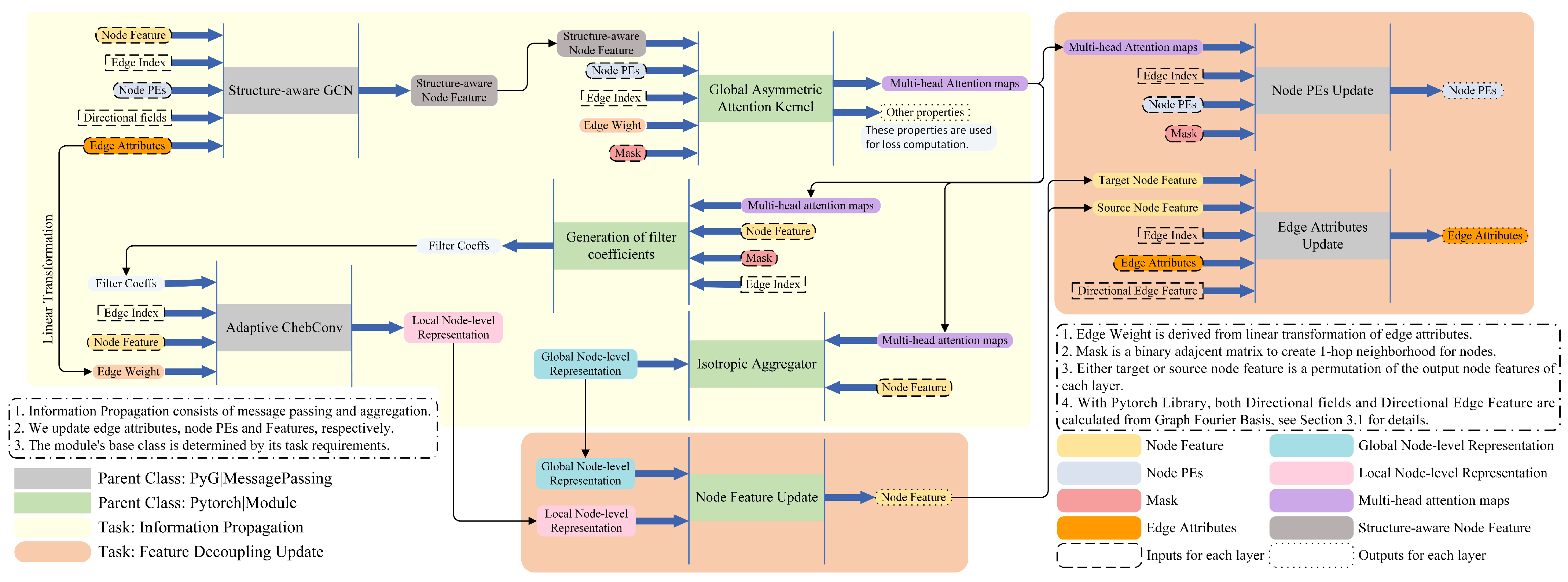
The first GT adaptively fuses multi-scale neighborhood aggregation through a channel attention mechanism, but lacks the global attention capability of the transformer architecture [24]. Dwivedi V.P. et al. first truly generalized the transformer to a discrete graph domain via node PE and feature update rules [14]. The node position encoding, serving as a soft inductive bias, is crucially aware of the diffusion distance between nodes in the GT. However, eigendecomposition is insensitive to sign flip and orthogonal transformation groups, resulting in the sign and basis being ambiguous. To overcome both of these issues, Lim et al. leveraged IGN [25] to achieve sign- and basis-invariant networks [26], ensuring the uniqueness of isomorphic graph node embeddings. The output of the parametric network violates the constraints of the Fourier basis. Ma et al. designed a non-parametric method for basis canonicalization [27]. Due to computational overhead, Dwivedi et al. employed random walks to obtain unique representations of node positions and decoupled the updates of edge and position embeddings [17]. Nevertheless, spatially structure-aware embeddings from random walks are less expressive than their spectral counterparts. Kreuzer et al. incorporated spectral features from eigendecomposition to balance computational complexity and model performance degradation [16]. Given that an equivalent complete set of graph Fourier bases from eigendecomposition is not enumerable, it is challenging for the model to fully determine both ambiguities. Additionally, Bo et al. leveraged a transformer encoder–decoder architecture to adaptively extract a task-related GLM, known as spectral GT, from spectral features [20].

Improving the effectiveness of attention maps can also observably improve the expression of GT. Traditional attention kernels, such as additive and dot-product attention kernels [28], have been proven to inadequately reveal the asymmetry between nodes from a single perspective [29,30]. Inspired by KSVD [31], Chen Y. et al. proposed an attention kernel that incorporates bidirectional asymmetry between nodes, thereby further enhancing the asymmetric expression of transformer [30]. Experiments have shown that the similarity of local neighborhood structures is crucial for evaluating the relative dependence between nodes, suggesting that the local neighborhood structure affects the attention score [18]. There is less research on directed GTs, whose bottleneck is the lack of a valid and universal directed node PE. Research on directed GTs remains relatively sparse, with a key bottleneck being the lack of an effective and universal directed node PE. Geisler et al. introduced the magnetic GLM to describe the biased connections between nodes and performed aggregation on both the imaginary and real parts separately through GTs [32]. However, the method for feature processing lacks geometric justification, resulting in suboptimal performance.

3. Proposed Model

For node-level graph representation learning, DSGT fruitfully integrates GT and directed GNN with the ability to approximate an arbitrary-order filter. As shown in Figure 1, the DSGT is a two-stage model, including preprocessing and forward inference.

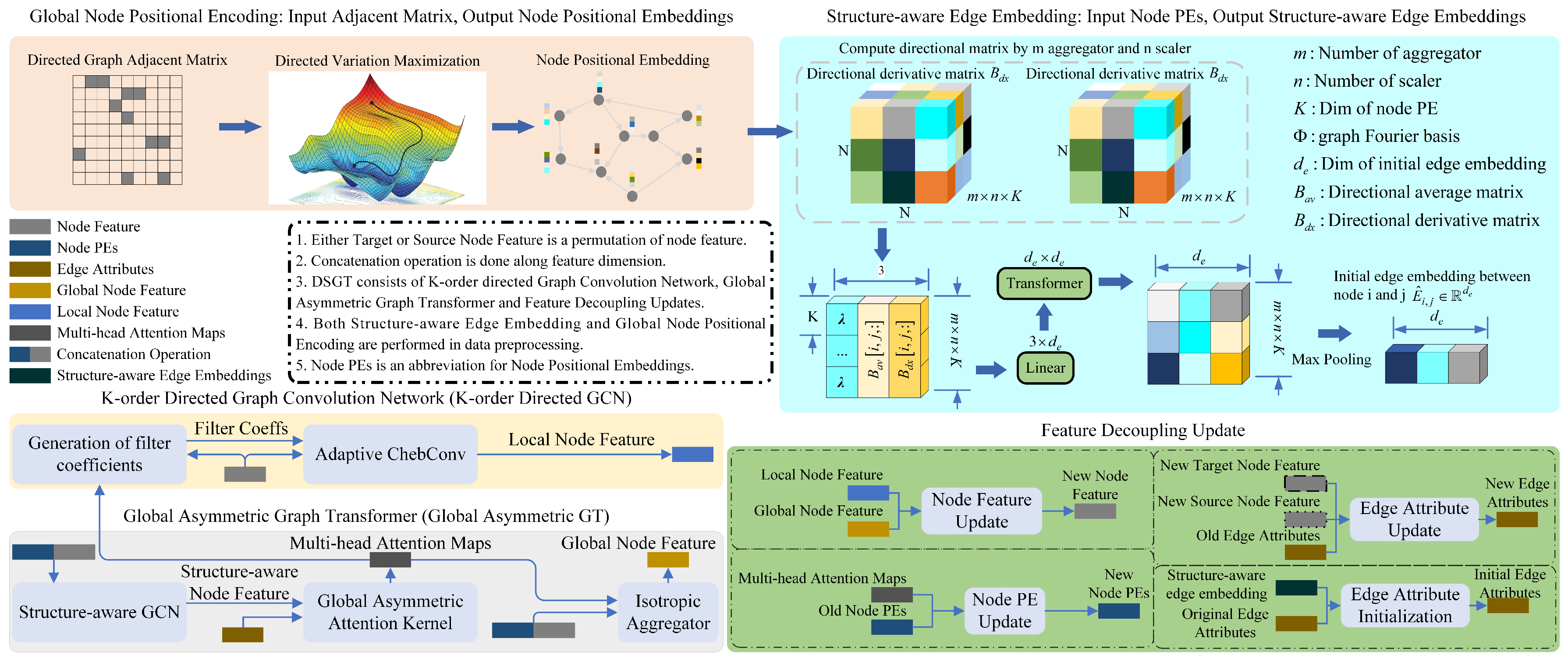
3.1. Graph Preprocessing

This section primarily elaborates on node PE and the initialization of structure-aware features for the edge. Graph data consist of graph topology and node features, which fall within the domain of irregular data. The graph topology describes the complex and flexible relationships between nodes, meaning that reordering the graph nodes results in a series of equivalent isomorphic graphs. Unlike grid data, the importance of nodes within the graph topology under different graph patterns is unique to them. Additionally, to respect the dominant direction of signal propagation under different graph frequencies, the graph connectivity under various graph frequencies is used as the initial feature for edges. To some extent, the initial edge features and global positional encoding of nodes can help to improve their expression in specific tasks.

3.1.1. Global Node Positional Encoding

To diversify directed graph patterns, the graph frequency is expected for an arithmetic sequence across as wide a frequency band as possible. Specifically, a two-stage optimization strategy is employed: first, the spectral radius and corresponding graph Fourier basis are determined by maximizing the directed total variation, and then, a set of complete Fourier bases is identified, with the corresponding graph frequencies as evenly distributed across the entire frequency band as possible. The node PE of fixed dimensions is derived from a complete set of graph Fourier bases.

$${\widehat{p}}_i=\mathrm{MLP}\left(\mathrm{Concat}\left(\mathbf{\lambda },{\mathbf{u}}_i\right)\right)P^{\left(0\right)}={\mathrm{GP}}_1\left(\mathrm{Transformer}\left(\widehat{P}\right)\right)$$

(1)

In Equation (1), the first-layer $d_p$-dimensional node PE $P^{\left(0\right)}\in {\mathbb{R}}^{N\times d_p}$, the frequency spectrum of the directed graph $\mathbf{\lambda }=\{{\lambda }_k,k=1,\cdots ,N\}\in {\mathbb{R}}^N$, and the importance of $i_{th}$ under graph frequency ${\mathbf{u}}_i=\{u_k^i,k=1,\cdots ,N\}\in {\mathbb{R}}^N$. The $N\times 2$-dimensional tensor is obtained via $\mathrm{Concat}(·)$ for each node. ${\mathrm{GP}}_i(·)$ is the global pooling operation to the $i_{th}$ dimension of the tensor. $\mathrm{MLP}:{\mathbb{R}}^2\to {\mathbb{R}}^{d_p}$; $\mathrm{Transformer}:{\mathbb{R}}^{d_p}\to {\mathbb{R}}^{d_p}$. The total variation is used to measure the smoothness of the node signal variations on the graph topology, quantifying the expected value of the discrete derivatives of graph signals, which can be used to define graph frequencies. The directed and undirected total variations are separately formulated as $\mathrm{DV}\left(x\right)={\sum }_{i,j=1}^N{A}_{ij}{\left[x_i-x_j\right]}_{+}^2$ and $\mathrm{TV}\left(x\right)=x{L}^{T}x={\sum }_{i=1,j>i}^N{A}_{ij}{\left[x_i-x_j\right]}^2$, where ${\left[x\right]}_{+}^2={\left({\left[x\right]}_{+}\right)}^2={(max(0,x))}^2$. For a self-adjoint adjacent matrix A, either $A_{ij}{\left[x_i-x_j\right]}_{+}^2$ or $A_{ji}{\left[x_j-x_i\right]}_{+}^2$ is zero if $A_{ij}=A_{ji}\ne 0$; in other words, $\mathrm{TV}\left(x\right)\equiv \mathrm{DV}\left(x\right)$, suggesting that the method for node PE is also applicable for undirected graphs. Notably, the total variation is insensitive to sign and permutation, which implies that there are no ambiguities for the definition of directed node PE. The expected frequencies follow an arithmetic progression, namely $f_k=\mathrm{DV}\left(u_k\right)={\displaystyle \frac{k-1}{N-1}}{f}_{max},k=1,\cdots ,N$, where $f_{max}$ is the spectral radius/largest frequency of the directed graph. The uniqueness of the frequency avoids basis ambiguity. First, the graph Fourier basis of the largest frequency is obtained through the maximum directed total variation and ensures the frequency band. Second, a group of approximately evenly distributed spectral features is the solution to the minimum spectral dispersion function across the frequency band.

$$\begin{array}{cc}\hfill & \underset{u}{min}-\mathrm{DV}\left(u\right)\mathrm{s}.\mathrm{t}.u^{T}u=1\hfill \\ \hfill & \underset{U}{min}\varphi \left(U\right)=\delta \left(U\right)+{\displaystyle \frac{\lambda }{2}}\left({∥u_1-u_{min}∥}^2+{∥u_N-u_{max}∥}^2\right)\hfill \\ \hfill & \mathrm{s}.\mathrm{t}.U^{T}U=I_N,\delta \left(U\right)=\sum _{i=1}^{N-1}{\left[\mathrm{DV}\left(u_{i+1}\right)-\mathrm{DV}\left(u_i\right)\right]}^2\hfill \end{array}$$

(2)

In Equation (2), $u_{min}={\mathbf{1}}_N/\sqrt{N}$ is the pattern of uniform diffusion and is orthogonal with $u_{max}$ (Proposition 4 [22]). The orthogonal constraint causes non-convex optimization. Wen et al. proposed a feasible iterative strategy for processing an orthogonality-preserved optimization problem with the form of ${min}_{U\in {\mathbb{R}}^{N\times M}}\Phi \left(U\right)$ s.t. $U^{T}U=I_M$. The iterative method for Equation (2) is shown in Algorithms 1 and 2. For each iteration, the step size is chosen by Algorithm 3 to satisfy the strong Armijo–Wolfe conditions. Ultimately, we can obtain the abundant graph patterns by optimizing objectives in Equation (2).

Algorithm 1 Directed variation maximization.

Input:  Adjacency matrix $A\in {\mathbb{R}}^{N\times N}$ and arbitrarily positive $ϵ>0$ Output:  Maximum graph frequency $f_{max}$ and corresponding graph Fourier basis ${\mathbf{u}}_{max}$   1: Initialize $k=0$ and unit-norm ${\mathbf{u}}_0\in {\mathbb{R}}^N$ at random   2: while $\parallel {\mathbf{u}}_k-{\mathbf{u}}_{k-1}\parallel \le ϵ$ do   3:     Evaluate the objective $\varphi \left({\mathbf{u}}_k\right)=$ −DV$\left({\mathbf{u}}_k\right)={\sum }_{i,j=1}^N{A}_{ij}{[x_i-x_j]}_{+}^2$   4:     Compute the gradient of the objective function $\overline{g}=\nabla$DV$\mathbf{u}\in {\mathbb{R}}^N$, the $i_{th}$ element of which is ${\overline{g}}_i=2\left(A_{:,i}^T{\left[u-u_i{1}_N\right]}_{+}-A_{i,:}{\left[u_i{1}_N-u\right]}_{+}\right),1\le i\le N$   5:     Compute the skew-symmetric matrix ${\mathbf{B}}_k={\overline{g}}_k{\mathbf{u}}_k^T-{\mathbf{u}}_k{\overline{g}}_k^T\in {\mathbb{R}}^{N\times N}$   6:     Select the step length ${\tau }_k$ of the $k_{th}$ iteration by Algorithm 1 or 3   7:     Update ${\mathbf{u}}_{k+1}\left({\tau }_k\right)={({\mathbf{I}}_N+{\displaystyle \frac{{\tau }_k}{2}}{\mathbf{B}}_k)}^{-1}({\mathbf{I}}_N-{\displaystyle \frac{{\tau }_k}{2}}{\mathbf{B}}_k){\mathbf{u}}_k$   8:     Update the index of iteration $k\leftarrow k+1$   9: end while 10: Return ${\mathbf{u}}_{max}={\mathbf{u}}_k$ and $f_{max}=$DV$\left({\mathbf{u}}_{max}\right)$

Algorithm 2 Spectral dispersion minimization.

Input:  Adjacency matrix $A\in {\mathbb{R}}^{N\times N}$ and arbitrarily positive $ϵ>0$, minimum and maximum graph frequency ${\mathbf{u}}_{min}={\displaystyle \frac{1}{\sqrt{N}}}{\mathbf{1}}_N,{\mathbf{u}}_{max}$ from the directed variation maximization algorithm, and regularization coefficient of the objective function $\lambda \in (0,1)$ Output:  A set of graph Fourier bases $\{{\mathbf{u}}_i,i=\{2,\cdots ,N-1\}\}$ whose corresponding graph frequencies approximate the arithmetic sequence   1: Initialize $k=0$ and orthonormal ${\mathbf{U}}_0\in {\mathbb{R}}^{N\times N}$ at random   2: while $\parallel {\mathbf{U}}_k-{\mathbf{U}}_{k-1}{\parallel }_F\le ϵ$ do   3:     Evaluate the objective with a measure of the constraint violations $\varphi \left(U\right)=\delta \left(U\right)+{\displaystyle \frac{\lambda }{2}}\left({∥u_1-u_{min}∥}_2^2+{∥u_N-u_{max}∥}_2^2\right)$, where, $\delta \left(U\right)={\sum }_{i=1}^{N-1}{\left[\mathrm{DV}\left(u_{i+1}\right)-\mathrm{DV}\left(u_i\right)\right]}_2^2$   4:     Compute the gradient of the objective function $G=\nabla \varphi \left(U\right)\in {\mathbb{R}}^{N\times N}$, the rows of which are $$\begin{array}{c}{G}_{1,:}=\left[\mathrm{DV}\left(u_1\right)-\mathrm{DV}\left(u_2\right)\right]\overline{g}\left(u_1\right)+\lambda \left(u_1-u_{min}\right)\hfill \\ G_{i,:}=\left[2\mathrm{DV}\left(u_i\right)-\mathrm{DV}\left(u_{i+1}\right)-\mathrm{DV}\left(u_{i-1}\right)\right]\overline{g}\left(u_1\right),1\le i\le N\hfill \\ G_{N,:}=\left[\mathrm{DV}\left(u_{N-1}\right)-\mathrm{DV}\left(u_N\right)\right]\overline{g}\left(u_N\right)+\lambda \left(u_N-u_{max}\right)\hfill \end{array}$$   5:     Compute the skew-symmetric matrix ${\mathbf{B}}_k=G_k{\mathbf{U}}_k^T-{\mathbf{U}}_k{G}_k^T\in {\mathbb{R}}^{N\times N}$   6:     Select the step length ${\tau }_k$ of the $k_{th}$ iteration by Algorithm 1 or 3   7:     Update ${\mathbf{U}}_{k+1}\left({\tau }_k\right)={({\mathbf{I}}_N+{\displaystyle \frac{{\tau }_k}{2}}{\mathbf{B}}_k)}^{-1}({\mathbf{I}}_N-{\displaystyle \frac{{\tau }_k}{2}}{\mathbf{B}}_k){\mathbf{U}}_k$   8:     Update the index of iteration $k\leftarrow k+1$   9: end while 10: Return $\widehat{\mathbf{U}}={\mathbf{U}}_k$ and $f_i=$DV$\left({\mathbf{U}}_{:,i}\right),1<i<N$

Algorithm 3 Non-monotone curvilinear search algorithm.

Input:  Maximum step length ${\tau }_{max}$; minimum step length ${\tau }_{min}$; hyperparameters $0<c_1<c_2<1$, where generally, $c_1={10}^{-4},c_2=0.9$; the objective function $\mathcal{F}\left(X\right)$ and its gradient ${\nabla }_X\mathcal{F}\left(X\right),\delta =0.1,\eta =0.85,ϵ={10}^{-5}$; chosen initial step length $\tau >0,{\tau }_{\max }={10}^4,{\tau }_{\min }={10}^{-4},{\tau }_{\mathrm{init}}={10}^{-3}$; maximum number of loop $L_{\max }=25,Q_0=1,C_0=\mathcal{F}\left(X_0\right)$; initial point $X_0$ in the Stiefel manifold Output:  The step length ${\tau }^{*}$ which satisfies the condition   1: function VariableUpdate($X_k,\mathcal{F},{\nabla }_X\mathcal{F},\tau$)   2:     $N,K=X$.shape   3:     if $N>2\times K$ then   4:         $U=[\nabla \mathcal{F}\left(X_k\right),X_k],V=[X_k,-\nabla \mathcal{F}\left(X_k\right)]$   5:         $X_{k+1}=X_k-\tau \times U{(I_{2K}+0.5\tau \times V^{T}U)}^{-1}{V}^{T}U$   6:     else   7:         $A=\nabla \mathcal{F}\left(X_k\right)X_k^T-X_k\nabla \mathcal{F}{\left(X_k\right)}^T$   8:         $X_{k+1}={(I_N+0.5\tau \times A)}^{-1}(I_N-0.5\tau \times A)X_k$   9:     end if 10:     return $X_{k+1}$ 11: end function 12: while $\parallel \nabla \mathcal{F}\left(X_k\right){\parallel }_2^2>ϵ$ do 13:     while $\mathcal{F}\left(Y_k\left(\tau \right)\right)\ge C_k+c_1\tau \nabla \mathcal{F}\left(Y_k\left(0\right)\right)$ do 14:         Scale step length $\tau$ to satisfy the condition, namely, $\tau \leftarrow \delta \times \tau$ 15:         if current loop index >= $L_{\max }$ and $\parallel \nabla \mathcal{F}\left(X_k\right){\parallel }_2^2>ϵ$ then 16:            Sample $\tau \sim \mathcal{N}(0,1)$ 17:            break 18:         end if 19:     end while 20:     $X_{k+1}=$ VariableUpdate$(X_k,\mathcal{F},\nabla \mathcal{F}),Q_{k+1}=\eta Q_k+1$ 21:     $C_{k+1}=(\eta Q_k{C}_k+\mathcal{F}\left(X_{k+1}\right))/Q_{k+1}$ 22:      Update ${\tau }_{k+1}$ by alternating between the following two methods: $$\begin{array}{c}\left(1\right){\tau }_{k,1}={\displaystyle \frac{\mathrm{tr}\left({\left(S_{k-1}\right)}^T{S}_{k-1}\right)}{\left|\mathrm{tr}\left({\left(S^{n-1}\right)}^T{Y}_{k-1}\right)\right|}}\left(2\right){\tau }_{k,2}={\displaystyle \frac{\left|\mathrm{tr}\left({\left(S_{k-1}\right)}^T{Y}_{k-1}\right)\right|}{\mathrm{tr}\left({\left(Y_{k-1}\right)}^T{Y}_{k-1}\right)}}\hfill \\ \mathrm{which},S_{k-1}=X_k-X_{k-1},Y_{k-1}=\nabla \mathcal{F}\left(X_k\right)-\nabla \mathcal{F}\left(X_{k-1}\right)\hfill \end{array}$$ 23:     Set $\tau =max(min({\tau }_{k+1},{\tau }_{max}),{\tau }_{min})$ 24:     if $k>=L_{\max }$ then 25:         break 26:     else 27:         $k\leftarrow k+1$ 28:     end if 29: end while 30: Return a feasible step length ${\tau }^{*}={\tau }_{k+1}$

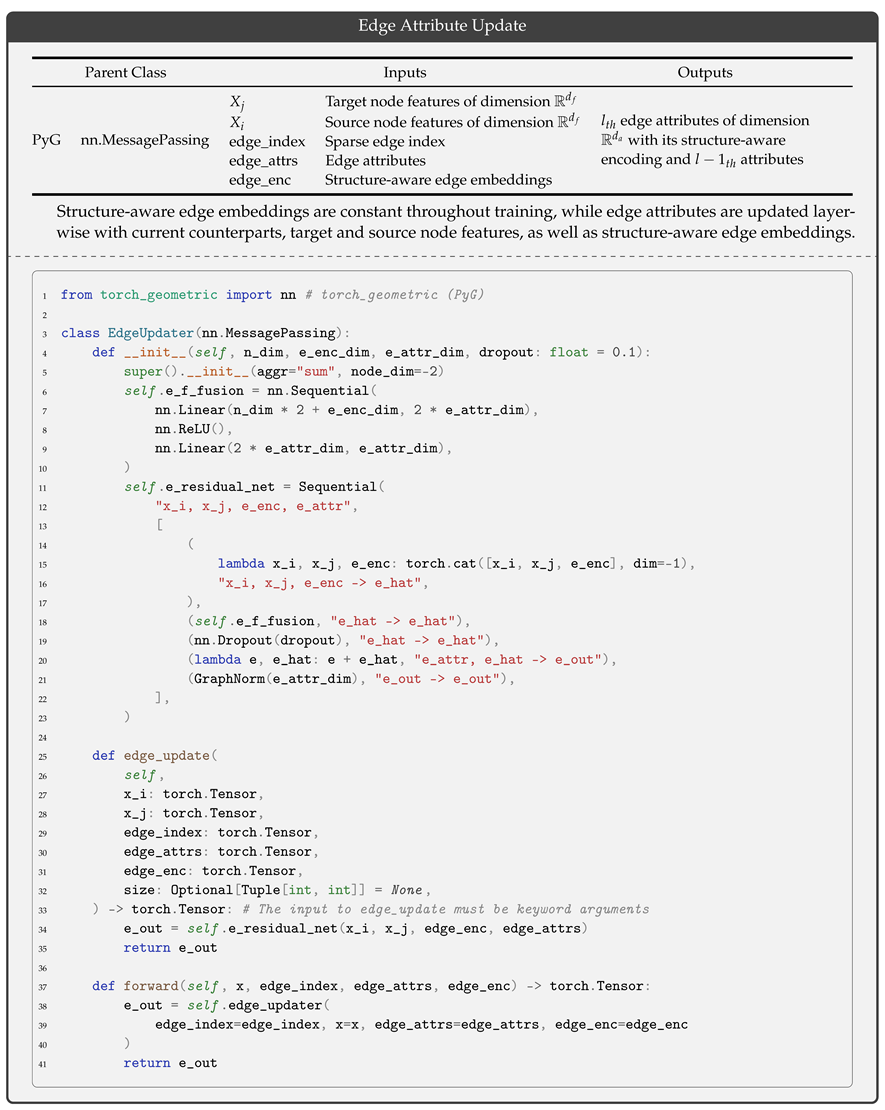
3.1.2. Structure-Aware Edge Embedding

Directional derivative and smoothing operators represent the global pattern of information flow, deriving from the difference of graph Fourier bases. Subsequently, graph frequencies, derivative, and smoothing operators are superimposed along a new dimension to obtain a 2D tensor that encapsulates the trend of information flow for each edge. Afterwards, the 2D tensor is transformed into a one-dimensional initial edge feature through an MLP and a transformer successively. The derivative of continuous signal provides information about the direction and intensity of its propagation. For discrete graph domains, the graph Fourier basis behaves similarly to the sine and cosine waves in continuous domains. The derivative of graph Fourier basis reflects the directional flow under the graph pattern. If we hope to further smooth discrete gradient of graph, the arcsine function can be used to postprocess the derivative.

$$F^k=\nabla u_k\mathrm{or}\nabla arcsin\left({\displaystyle \frac{u_k}{max\left(\left|u_k\right|\right)}}\right)$$

(3)

In Equation (3), the graph Fourier basis $u_k\in {\mathbb{R}}^N$, the directional field $F^k\in {\mathbb{R}}^{N\times N}$, and the discrete derivative operator is ∇. In Appendix A and Equation (11) of [33], the author provides three aggregators (soft and hard softmax aggregators and a center-balanced aggregator) and scalers (degree-attenuation, degree-amplification, and identity), suggesting that $B_{\mathrm{av}}^k,B_{\mathrm{dx}}^k\in {\mathbb{R}}^{(9\times K)\times N\times N}$ is the nine-dimensional tensor for the $k_{th}$ graph Fourier basis. When the number of graph Fourier bases is K, the dimension of the directional derivative $B_{\mathrm{av}}$ and smoothing matrix $B_{\mathrm{dx}}$ is $(9\times K)\times N\times N$. Consideration of either the graph frequency or graph Fourier basis is insufficient to distinguish non-isomorphic graphs. The method for structure-aware edge embedding is formulated as follows.

$$\begin{array}{cc}\hfill {\tilde{e}}_{ij}& =\mathrm{Concat}(B_{\mathrm{av}}[:,i,j],B_{\mathrm{dx}}[:,i,j],\Lambda )\hfill \\ \hfill {\overline{e}}_{ij}& ={\mathrm{GP}}_1\left(\mathrm{Transformer}\left({\tilde{e}}_{ij}^T{W}_0\right)\right)e_{ij}^0=\mathrm{Concat}({\overline{e}}_{ij},e_{ij})\hfill \end{array}$$

(4)

In Equation (4), each element of $\{{\lambda }_i,i=1,\cdots ,K\}$ is replicated nine times to form a new $9\times K$-dimensional vector linear transformation matrix $W_0\in {\mathbb{R}}^{3\times d_e}$. The transformer encoder $\mathrm{Transformer}:{\mathbb{R}}^{K\times d_e}\to \mathbb{K}\times {\mathbb{d}}_{\mathbb{e}}$ captures the dependence of K features to encode context information, and then, the global maximum pooling ${\mathrm{GP}}_2:{\mathbb{R}}^{K\times d_e}\to {\mathbb{R}}^{d_e}$ performs dimensional reduction. The ${\overline{e}}_{ij}\in {\mathbb{R}}^{d_e}$ is the structure-aware edge feature between the $i_{th}$ and $j_{th}$ nodes. The structure-aware edge feature ${\overline{e}}_{ij}\in {\mathbb{R}}^{d_e}$ and attribute $e_{ij}\in {\mathbb{R}}^{d_a}$ are stacked to obtain the initial edge feature $e_{ij}^0\in {\mathbb{R}}^{d_e+d_a}$.

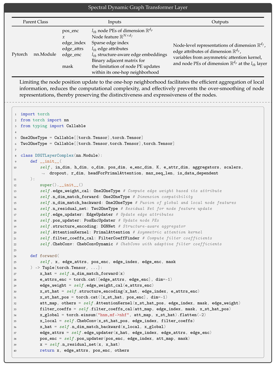
3.2. Directed Spectral Graph Transformer

The directed spectral graph transformer (DSGT) consists of a global asymmetric graph transformer (GT), a K-order directed graph convolution network (GCN), and a feature decoupling update. Specifically, the global asymmetric GT computes an attention map and then performs global aggregation from which the coefficients of the K-order GCN are extracted. Subsequently, the K-order directed GCN aggregates local information. Finally, inspired by the research of Dwivedi V. et al. [17], the model decouples the update processes for structure (node and edge attributes) and position (global node PE).

3.2.1. Global Asymmetric Graph Transformer

As shown in Appendix A.3, traditional attention kernels have been proved to underexploit the asymmetric relationships between nodes [29]. The global asymmetric graph transformer includes structure encoding, PrimalAttention, and global aggregation. Specifically, the first-order DGN [33] is performed to embed structural information into node attributes. Then, the asymmetric attention map is computed from PrimalAttention and edge attributes. Finally, the global aggregation is performed to obtain global node-level representations. Directional convolution is performed via DGN as follows:

$$\begin{array}{cc}\hfill {\widehat{X}}^{\left(l\right)}& =\mathrm{MLP}\left(\mathrm{Concat}\left(D_{\mathrm{in}}^{-1}A{X}^{\left(l\right)},{\left\{{\tilde{X}}_k^{\left(l\right)}\right\}}_{k=1,\cdots ,K}\right)\right)\hfill \\ \hfill {\overline{X}}_{\alpha ,i,k}^{\left(l\right)}& =\left(\widehat{S}(D_{\mathrm{in}},\alpha )·B_{\mathrm{av}}^k[:,:,i]\odot A\right)X^{\left(l\right)}\parallel \left(\widehat{S}(D_{\mathrm{in}},\alpha )·B_{\mathrm{dx}}{[:,:,i]}^k\odot A\right)X^{\left(l\right)}\hfill \\ \hfill {\tilde{X}}_k^{\left(l\right)}& =\mathrm{Concat}\left(\left\{{\overline{X}}_{\alpha ,i,k},\alpha =-1,0,+1,i=1,2,3\right\}\right)\hfill \\ \hfill \widehat{S}(D,\alpha )& =\mathrm{diag}\left({\left\{S(D_{ii},\alpha )\right\}}_{i=\{1,\cdots ,N\}}\right),\mathrm{where},\left\{\begin{array}{c}S(d,\alpha )={\left({\displaystyle \frac{log(d+1)}{\delta }}\right)}^{\alpha }\hfill \\ \delta ={\displaystyle \frac{1}{N}}\sum _{i=1}^{N}ln\left(D_{ii}+1\right)\hfill \\ \alpha \in [-1,+1]\hfill \end{array}\right.\hfill \end{array}$$

(5)

In Equation (5), ⊙ is the element-wise product, and $·\parallel ·$ is the concatenation of node features. The aggregators and scalers are set the same as in Section 3.1.2, where $\left\{X^{\left(l\right)},{\widehat{X}}^{\left(l\right)}\right\}\in {\mathbb{R}}^{N\times d_f}$, $d_f$ is the dimension of the node feature, and N is the number of nodes in the directed graph. For each graph Fourier basis, the aggregation matrix of three aggregators $\left\{B_{\mathrm{av}}^k,B_{\mathrm{dx}}^k\right\}\in {\mathbb{R}}^{N\times N\times 3}$, and the scalers include the degree-attenuation $\widehat{S}(D,-1)\in {\mathbb{R}}^{N\times N}$, the degree-amplification $\widehat{S}(D,+1)$, the identity $\widehat{S}(D,0)=I_N$, and the concatenation of node features after aggregation ${\tilde{X}}_k^l\in {\mathbb{R}}^{N\times (9\times d_f)}$. We stack the node features and go through $\mathrm{MLP}:{\mathbb{R}}^{N\times ((9\times K+1)\times d_f)}\to {\mathbb{R}}^{N\times d_f}$ to obtain the $l_{th}$ node representation ${\mathbb{R}}^{N\times d_f}$. The evaluation of attention scores for structure-aware node features is as follows. The mathematical formulation of the asymmetric attention kernel is shown in Appendix C.2.

$$\begin{array}{ccc}\hfill e\left(X_i^{\left(l\right)}\right)& ={\left(f{\left(X\right)}^T{W}_e\right)}^T{g}_q\left(q\left(X_i^{\left(l\right)}\right)\right)\hfill & \hfill r\left(X_j^{\left(l\right)}\right)={\left(f{\left(X\right)}^T{W}_r\right)}^T{g}_k\left(k\left(X_j^{\left(l\right)}\right)\right)\end{array}$$

(6)

$$\begin{array}{ccc}\hfill {\mathrm{ATT}}_{i,:}& =\mathrm{Softmax}\left({\widehat{ATT}}_{i,:}\right)\hfill & \hfill {\widehat{ATT}}_{i,j}=\mathrm{Concat}\left(e\left(X_i^{\left(l\right)}\right),r\left(X_j^{\left(l\right)}\right)\right)\end{array}$$

(7)

In Equation (6), $q\left(X_i^{\left(l\right)}\right)=W_q{X}_i^{\left(l\right)}\in {\mathbb{R}}^{d_q}$ and $k\left(X_j^{\left(l\right)}\right)=W_k{X}_j^{\left(l\right)}\in {\mathbb{R}}^{d_k}$ are samples of query and key space, respectively, with $g_q(·):{\mathbb{R}}^{d_p}\to {\mathbb{R}}^d$ and $g_k(·):{\mathbb{R}}^{d_k}\to {\mathbb{R}}^d$ ensuring dimension compatibility. The injection of data dependence transforms the projection matrix $W_e,W_r\in {\mathbb{R}}^{N\times s}$ to its revised counterpart $f{\left(X^{\left(l\right)}\right)}^T{W}_e=W_{e|x},f{\left(X^{\left(l\right)}\right)}^T{W}_r=W_{r|x}\in {\mathbb{R}}^{p\times s}$, where $f\left(X^l\right)={\widehat{X}}^{\left(l\right)}{R}^T\in {\mathbb{R}}^{N\times p}$ is derived from the random projection of $X^{\left(l\right)}$ according to the Johnson–Lindenstrauss lemma; the random projection matrix $R\in {\mathbb{R}}^{d_f\times p}$, each element of which follows a standard normal distribution, namely $R_{ij}\sim \mathcal{N}(0,1)$. $e\left(X_i^{\left(l\right)}\right),r\left(X_j^{\left(l\right)}\right)\in {\mathbb{R}}^s$, are, separately, the s projection scores of the $i_{th}$ value and $j_{th}$ key sample in the key and value feature space. The edge feature is integrated into the attention map $\mathrm{ATT}\in {\mathbb{R}}^{N\times N}$ through the linear transformation matrix $W_1\in {\mathbb{R}}^{2s},W_2\in {\mathbb{R}}^{d_e+d_a}$. Global aggregation with the in-degree scaler [18] is performed using the weighted sum of neighborhood features.

$$X_g^{l+1}=\sigma \left(D^{-1/2}·\mathrm{ATT}·X^l\right)$$

(8)

In Equation (8), the global node representation at the ${l+1}_{th}$ layer $X_g^{l+1}\in {\mathbb{R}}^{N\times d_f}$ is obtained by aggregating $X^{\left(l\right)}\in {\mathbb{R}}^{N\times d_f}$ using the global asymmetric GT. In the global asymmetric GT, the optimal projection matrices $W_{e|x},W_{r|x}$ along which mutual information is greatest are obtained through the minimum regularization term in the total loss. The optimization objective for the self-attention kernel can be formulated as follows [31]:

$$\begin{array}{c}\underset{W_e,W_r,e_i,r_j}{max}J={\displaystyle \frac{1}{2}}\sum _{i=1}^N{e}_i^T\Lambda e_i+{\displaystyle \frac{1}{2}}\sum _{j=1}^N{r}_j^T\Lambda r_j-\mathrm{Tr}\left(W_{e|x}^T{W}_{r|x}\right)\hfill \\ \mathrm{s}.\mathrm{t}.e_i=e\left(X_i^{\left(l\right)}\right)={\left(f{\left(X\right)}^T{W}_{e|x}\right)}^T{\phi }_q\left(X_i\right)r_j=r\left(X_j^{\left(l\right)}\right)={\left(f{\left(X\right)}^T{W}_{r|x}\right)}^T{\phi }_k\left(X_j\right)\hfill \end{array}$$

(9)

In Equation (9), $\Lambda \in {\mathbb{R}}^{s\times s}$ is the diagonal matrix filled by Lagrange multipliers, which represents the penalty intensity for objects that violate the constraints. Generally, the number of principal components s is not larger than the dimension p; namely, $s\le p$. The feasible solution to the optimization objective in Equation (9) is formulated as the least-square support vector machine (LSSVM) (Appendix A.2). We demonstrate that the objective in Equation (9) is constantly equal to 0 if the stationary condition in Equation (A6) is workable (Appendix A.2). To satisfy the stationary condition, the objective of the primal problem is formulated as a regularization term in the loss function. This goal is implemented using automatic differentiation libraries (e.g., PyTorch [34] and TensorFlow [35]). In Equation (10), the regularization term $J_a$ is expected to approach 0. Although GTs are confronted with the inability to unbiasedly approximate the frequency responses of the high-order filter, both K-order directed GCNs and GTs are complementary with each other such that a hybrid architecture model is crucially constructed.

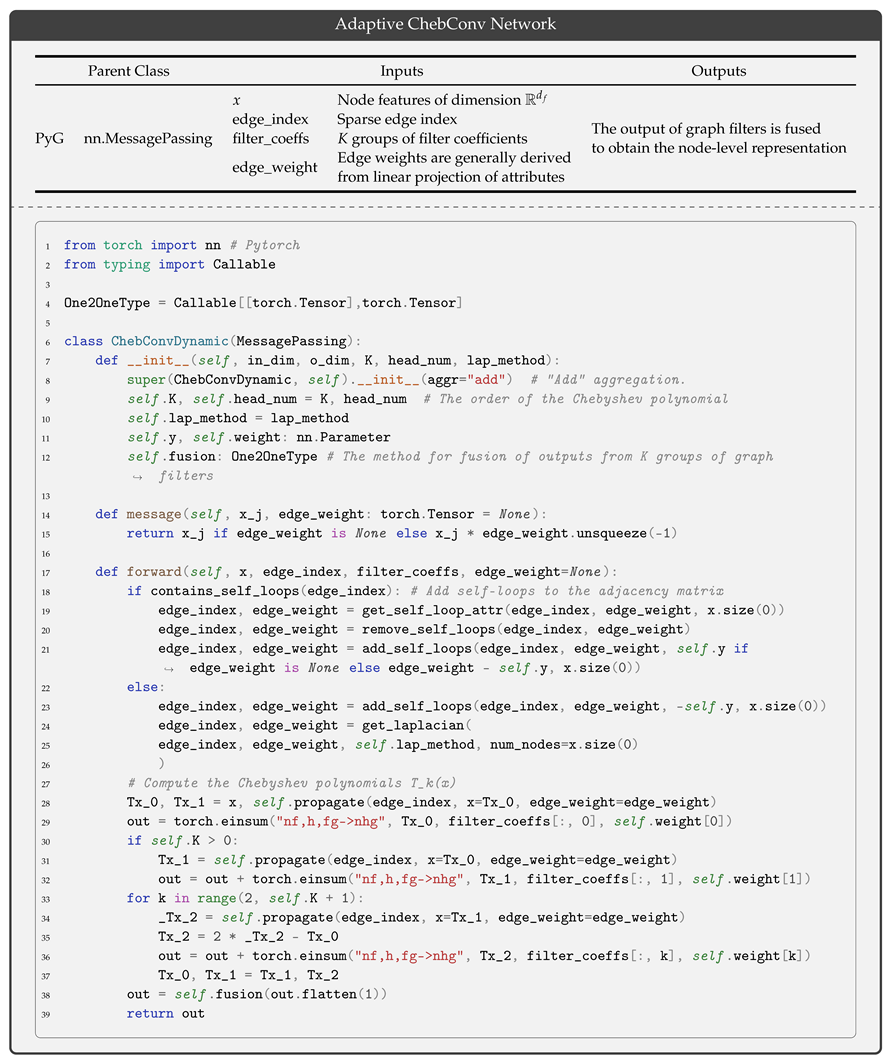
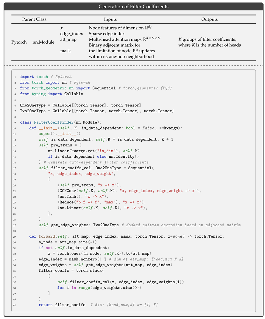
3.2.2. K-Order Directed Graph Convolution Network

The assumption for a self-adjoint GSO in the traditional spectral graph theory is not applicable for directed graphs. We elaborate the spectral graph theory completely defined in the directed graph and then construct directed spectral graph convolution based on the theory. Specifically, directed GLM is defined as $T=I_N-D_{\mathrm{in}}^{-1}A$ via graph diffusion [10], where the directed GLM T is not a self-adjoint matrix, suggesting that its frequency response is not described in the eigenspace of GLM T. However, the frequency response of the directed graph can be fully represented in the generalized eigenspace of GLM T. The generalized spectral features of the directed graph are obtained via Jordan decomposition.

In Equation (11), $m_{\lambda }$ is the algebraic multiplicity of the eigenvalue $\lambda$ of directed GLM T, satisfying $\left(T-\lambda ·I_N\right)·P_{\lambda }={\left[\left(T-\lambda ·I_N\right)·P_{\lambda }\right]}^{m_{\lambda }}=\mathbf{0}$. $P^{-1}TP=J$ is the Jordanization of GLM T, where the dyad of GLM T satisfies $P_{\lambda }=\left[v_{\lambda }^1,·,v_{\lambda }^{m_{\lambda }}\right]{\left[v_{\lambda }^1,·,v_{\lambda }^{m_{\lambda }}\right]}^T\in {\mathbb{R}}^{N\times N}$, where $\left\{v_{\lambda }^i,i=1,\cdots ,m_{\lambda }\right\}$ is a set of bases in the generalized feature subspace according to the eigenvalue $\lambda$[36]. In the generalized eigenspace, the polynomial of GLM T is formulated as follows:

$$\begin{array}{cc}\hfill & J_a\left(W_c,W_r,\Lambda \right)={\displaystyle \frac{1}{2}}\sum _{i=1}^N{e}_i^T\Lambda e_i+{\displaystyle \frac{1}{2}}\sum _{j=1}^N{r}_j^T\Lambda r_j-\mathrm{Tr}\left(W_e^T{W}_r\right)\hfill \\ \hfill & ={\displaystyle \frac{1}{2}}\sum _{i=1}^N\parallel {\left(W_{e|X}{\Lambda }^{1/2}\right)}^T{\phi }_q\left(X_i\right){\parallel }_2^2+{\displaystyle \frac{1}{2}}\sum _{j=1}^N\parallel {\left(W_{r|X}{\Lambda }^{1/2}\right)}^T{\phi }_k\left(X_j\right){\parallel }_2^2-\mathrm{Tr}\left(W_{e|X}^T{W}_{r|X}\right)\hfill \end{array}$$

(10)

$$\left(T-\lambda ·I_N\right)·P_{\lambda }=\sum _{\lambda }g\left(\lambda \right)P_{\lambda }+\sum _{\lambda }\left[\sum _{n=1}^{m_{\lambda }-1}{\displaystyle \frac{g^{\left(n\right)}\left(\lambda \right)}{n!}}{(T-\lambda ·I_N)}^n\right]P_{\lambda }$$

(11)

$$g\left(T\right)=\sum _{\lambda }g\left(\lambda \right)P_{\lambda }+\sum _{\lambda }\left[\sum _{n=1}^{m_{\lambda }-1}{\displaystyle \frac{g^{\left(n\right)}\left(\lambda \right)}{n!}}{\left(Y-\lambda ·I_N\right)}^n\right]P_{\lambda }$$

(12)

In Equation (12), the second term of $g\left(T\right)$ represents the difference in frequency response between a self-adjoint and no self-adjoint GSO. The sum of the dimensions of the feature subspace $m_{\lambda }$ is equal to the number of nodes N, namely ${\sum }_{\lambda }{m}_{\lambda }=N$. The polynomial of GLM T $g\left(T\right)$ is also formulated as a holomorphic functional calculus $g\left(T\right)={\displaystyle \frac{1}{2\pi i}}{\oint }_{\Gamma }g\left(z\right)·{(T-z·I_N)}^{-1}dz$, where $\Gamma$ is the curve enveloping all the eigenvalues of GLM T, and $g\left(z\right)$ is the polynomial of z. The Faber polynomial is the best for approximating any holomorphic function in the complex space. Fortunately, if all the eigenvalues are located inside the unit hypersphere, the Faber polynomial is equivalent to the Chebyshev polynomial [37]. Therefore, directed GLM T is normalized by the modulus of the spectral radius, namely $\tilde{T}=T/\parallel {\lambda }_{max}\parallel$. The faber polynomial of $g\left(T\right)$ is formulated as follows:

$$g_{\theta }\left(\tilde{T}\right)=\sum _{k=1}^K{\theta }_i{\tilde{T}}^i\approx \sum _{k=1}^K{\theta }_i{T}_k\left(\tilde{T}\right),\mathrm{where},\left\{\begin{array}{c}\mathit{\theta }=\mathrm{MLP}\left({\displaystyle \frac{1}{N}}\sum _{i=1}^N{X}_g^{(l+1)}[i,:]\right)\hfill \\ T_0\left(X\right)=I_N,T_1\left(X\right)=X\hfill \\ T_k\left(X\right)=2X·T_{k-1}\left(X\right)-T_{k-1}\left(X\right),k\ge 2\hfill \end{array}\right.$$

(13)

In Equation (13), the polynomial coefficients $\mathit{\theta }=[{\theta }_0,\cdots ,{\theta }_K]\in {\mathbb{R}}^{K+1}$ are obtained from global aggregation. The readout function is a successive component of mean pooling and MLP. $T_k\left(\tilde{T}\right)$ approximates the basis of the polynomial space ${\tilde{T}}^k$. For the Liouville theorem, an ideal filter for fully suppressing high-frequency noise does not exist; namely, $P_{\lambda }·g^{\left(n\right)}\left(\lambda \right)/n!\to 0$ is not possible as $\lambda \to 0$. To theoretically achieve the goal, we redefine GLM T in the punctured complex space $\mathbb{C}/y$ as $g_{\theta }\left(\tilde{T}\right)={\sum }_{k=1}^K{\theta }_i{\tilde{T}}^i\approx {\sum }_{k=1}^K{\theta }_i{T}_k\left(\tilde{T}\right)$, where $\tilde{T}={\displaystyle \frac{1}{∥{\lambda }_{max}∥}}T-y\times I_N$, and $y\in (0,1)$ is the singular point inside the unit hypersphere, which can adjust the behavior of the holomorphic functional calculus. Finally, local aggregation is performed through a K-order directed GCN.

$$X_l^{(l+1)}=\mathrm{FFN}\left(D_{\mathrm{in}}^{-1}·\sum _{k=1}^K{\theta }_i{T}_k\left(\tilde{T}\right){\widehat{X}}^l\right){\widehat{X}}^{\left(l\right)}=\mathrm{Concat}\left(X^{\left(l\right)},P^{\left(l\right)}\right)$$

(14)

In Equation (14), the $l_{th}$-layer forward feedback network $\mathrm{FFN}:{\mathbb{R}}^{d_f+d_p}\to {\mathbb{R}}^{d_f}$ is for dimension compatibility, and ${\widehat{X}}^{\left(l\right)}\in {\mathbb{R}}^{N\times d_f}$ is the concatenation of the $l_{th}$-layer node features $X^{\left(l\right)}\in {\mathbb{R}}^{N\times d_f}$ and node PE $P^{\left(l\right)}\in {\mathbb{R}}^{N\times d_p}$. Finally, we design the rules for decoupling edge attributes, and node feature and PE updates, which are key to improving training stability and reference efficiency.

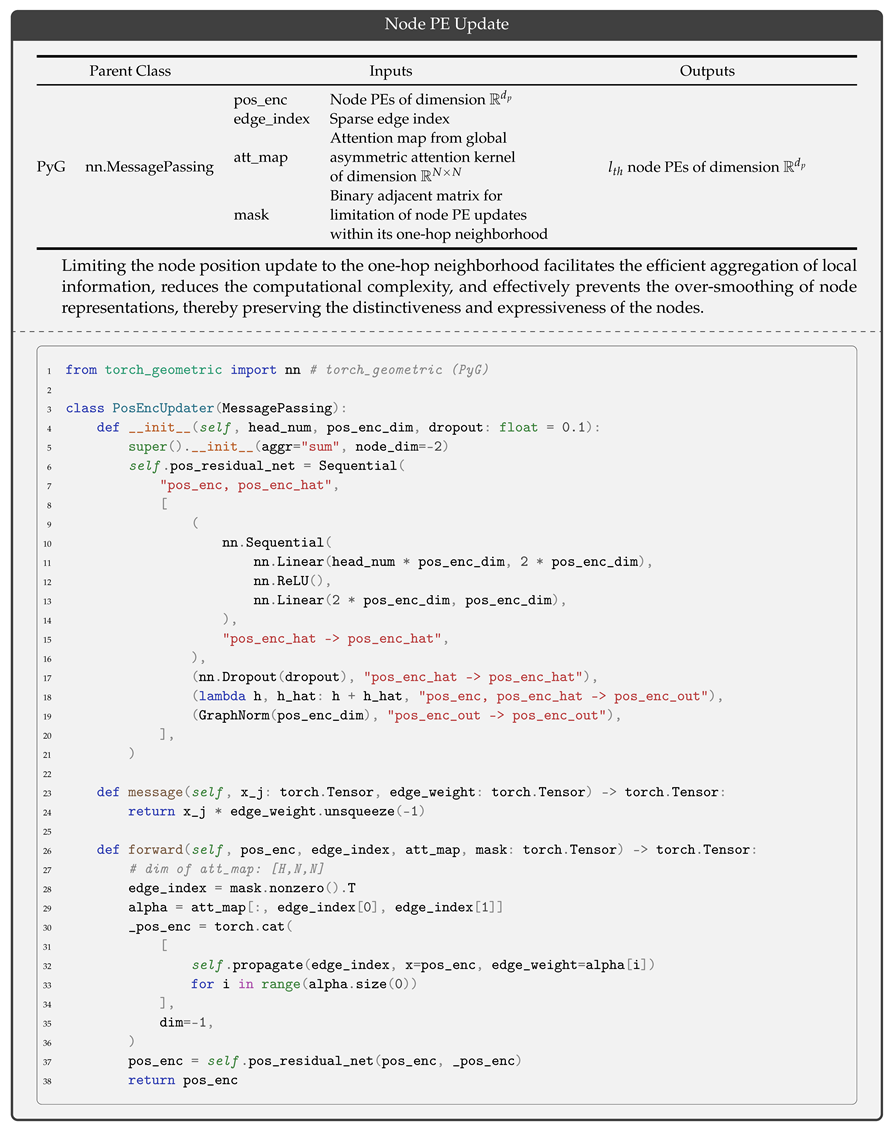
3.2.3. Feature Decoupling Update

Decoupling the update of structural features and positional coordinates helps to enhance the interpretability of the model’s inference process. Specifically, the fusion of the $l_{th}$-layer local and global node representation $X^{\left(l\right)}\in {\mathbb{R}}^{d_f}$ is formulated as ${\breve{X}}^{\left(l\right)}=\mathrm{MLP}\left(\mathrm{Concat}\left(X_g^{\left(l\right)},X_l^{\left(l\right)}\right)\right)$, where the multi-layer perceptron $\mathrm{MLP}:{\mathbb{R}}^{2d_f}\to {\mathbb{R}}^{d_f}$ is for dimension compatibility. The edge acts as the channel through which information flows in the graph, so its attribute is updated based on the feature of neighbor nodes, namely ${\breve{e}}_{kj}^{\left(l\right)}=\mathrm{MLP}\left(\mathrm{Concat}\left(x_k^{\left(l\right)},x_j^{\left(l\right)}\right)\right)$. Unlike structural updates, the node PE needs to reflect the $l_{th}$-layer diffusion distance between nodes. Because the attention map reflects the global connectivity of the graph, the update of the $l_{th}$-layer node PE is formulated as ${\breve{P}}^{\left(l\right)}=\mathrm{ATT}·P^{(l-1)}$. Additionally, GraphNorm [38] and residual connection are leveraged to achieve a deeper structure and abstracter representation.

$$H^{\left(l\right)}=\mathrm{Norm}\left(\mathrm{Dropout}\left({\breve{H}}^{\left(l\right)}\right)+H^{(l-1)}\right),\mathrm{where}\left\{\begin{array}{cc}\hfill {\breve{H}}^{\left(l\right)}& \in \left\{{\breve{X}}^{\left(l\right)},{\breve{P}}^{\left(l\right)},{\breve{e}}_{kj}^{\left(l\right)}\right\}\hfill \\ \hfill H^{(l-1)}& \in \left\{X^{(l-1)},P^{(l-1)},e_{kj}^{(l-1)}\right\}\hfill \end{array}\right.$$

(15)

In Equation (15), randomly inactivating some parameters via $\mathrm{Dropout}(·)$ can avoid overfitting and improve the robustness of DSGT; generally, the dropout ratio is set to 0.1.

3.3. End-to-End Optimization for DSGT

For node-level classification tasks, the multi-class joint probability distribution is obtained through an affine transformation and softmax operation.

$$\widehat{Y}=\mathrm{softmax}\left(X^{\left(L\right)}{W}_o^T\right)$$

(16)

In Equation (16), the linear transformation matrix $W_o\in {\mathbb{R}}^{d_f\times d_c}$, and $\mathrm{softmax}\left(x\right)={\displaystyle \frac{exp\left(x_i\right)}{{\sum }_{j}exp\left(x_j\right)}}$. The number of layers of DSGT is L. $\widehat{Y}\in {\mathbb{R}}^{N\times d_c}$ represents the probability of the node class, where $d_c$ is the number of classes. Our goal is to satisfy the stationary condition, force the node PE to form a coordinate system constrained by the graph topology, and obtain robust performance at the node level. To achieve these goals, the loss function is formulated as follows:

$$\mathcal{L}={\displaystyle \frac{1}{N}}\left(\sum _{i=1}^N{\mathcal{L}}_{\mathrm{cls}}\left({\widehat{Y}}_i,Y_i\right)+\eta \left(J_a\left(W_{e|X},W_{r|X},\Lambda \right)+J_e\left(\widehat{Y}\right)+J_p\left(P^{\left(L\right)}\right)\right)\right)$$

(17)

In Equation (17), $\widehat{Y}\in {\mathbb{R}}^{N\times d_c}$ and $Y_{ij}\in \{0,\cdots ,d_c-1\}$ are the joint probability distributions of the node class and ground-truth node label. The entropy regularization $J_e\left(\widehat{Y}\right)=-{\sum }_{i=0}^N{\sum }_{l=1}^{d_c}{\widehat{Y}}_{ij}ln\left({\widehat{Y}}_{ij}+ϵ\right)$ encourages uncertainty in the classification to a certain extent. The presence of $J_a(W_{e|X},W_{r|X},\Lambda )$ in Equation (17) satisfies the stationary condition of the optimization objective in Equation (A6). The regularization term for node PE $J_p\left(P^{\left(L\right)}\right)=1/d_p+\mathrm{Tr}\left({P^{\left(l\right)}}^T▵P^{\left(l\right)}\right)+\lambda /d_p\times \parallel {P^{\left(l\right)}}^T{P}^{\left(l\right)}-I_{d_p}{\parallel }_2^2$ constrains the node PE to form an orthogonal coordinate system, where $▵=I_N-D_{\mathrm{in}}^{-1}A\in {\mathbb{R}}^{N\times N}$ is the directed GLM and p is the final/$L_{th}$-layer node PE $P^{\left(L\right)}\in {\mathbb{R}}^{N\times d_p}$. The $L_{\mathrm{cls}}(·)$ is a multi-class cross-entropy loss function. The $\eta$ is a regularization coefficient; generally, $\eta =0.1$. The model was constructed using the PyTorch framework, and the parameters were updated using the Adam optimizer. The inference and optimization processes for the DSGT model are illustrated in Algorithm 4.

Algorithm 4 Supervised node-level embedding algorithm.

Input:  Adjacency matrix $A\in {\mathbb{R}}^{N\times N}$ and node feature matrix $X\in {\mathbb{R}}^{N\times d_f}$; layer number L; learning rate lr = ${10}^{-3}$; true node’s label $Y\in {\mathbb{R}}^N,y_i\in \{0,\cdots ,d_c-1\}$; label number $d_c$; total epoch number N Output:  Node feature matrix $X^L$; edge feature matrix $E^L$; and node relative position $P^L$ in the $L_{th}$/final layer   1: function Feature Engineering(adjacent matrix A)   2:     Compute directed graph frequencies $\{{\lambda }_k,k=,\cdots ,N\}$ and a complete set of Fourier basis $\{u_k,k=1,\cdots ,N\}$ from directed graph shift operator A, and get global positional encoding $P^{\left(0\right)}$ from them   3:     Compute directional smoothing matrix $B_{av}$ and derivative matrix $B_{dx}$ by the Fourier basis $\{u_k,k=1,\cdots ,N\}$, and then, initialize edge feature $E^{\left(0\right)}$ with graph spectrum $\{{\lambda }_i,i=1,\cdots ,N\}$ and them   4:     return edge feature matrix $E^{\left(0\right)}$ and positional embedding $P^{\left(0\right)}$   5: end function   6: function DSGT(node feature matrix $X^{\left(0\right)}$, edge feature ${\mathrm{matrix} }^{\left(0\right)}E$, node positional embeding $P^{\left(0\right)}$)   7:     for $k\in \{1,\cdots ,K\}$ do   8:         Compute global node feature matrix of $k_{th}$ layer $X_g^{(k+1)}$ using the global asymmetric graph transformer and the average loss of attention kernel $J_a(W_e,W_r,\Lambda )$ for each head   9:         Compute local node feature matrix of $k_{th}$ layer $X_l^{(k+1)}$ by K-order Directed Graph Convolution 10:         Update edge feature $E^{(k+1)}$, node feature $X^{(k+1)}$, and relative positional encoding $P^{(k+1)}$ with $X_g^{(k+1)},X_l^{(k+1)},E^{\left(k\right)}$, and $P^{\left(k\right)}$ 11:         $k\leftarrow k+1$ 12:     end for 13:     return output node feature matrix $X^{\left(L\right)}$ 14: end function 15: for current epoch $i\le N$ do 16:     $X^{\left(0\right)},A\leftarrow$ the $i_{th}$ subgraph of training dataset 17:     $E^{\left(0\right)},P^{\left(0\right)}=$ FEATURE ENGINEERING(A) 18:     $X^{\left(L\right)}=$DSGT($X^{\left(0\right)},E^{\left(0\right)},P^{\left(0\right)}$) 19:     Compute joint probability distribution of node’s multi-label $\widehat{Y}$ by affine transformation and softmax for $X^{\left(L\right)}$ and its entropy regularization $J_e\left(\widehat{Y}\right)$ 20:     Compute average loss function $\mathcal{L}={\displaystyle \frac{1}{N}}\left({\mathcal{L}}_{cls}(\widehat{Y},Y)+\eta {\mathcal{L}}_{reg}\right)={\displaystyle \frac{1}{N}}\left({\mathcal{L}}_{cls}(\widehat{Y},Y)+\eta \left(J_a(W_e,W_r,\Lambda )+J_e\left(\widehat{Y}\right)\right)\right)$ 21:     Carry out backpropagation algorithm for total loss $\mathcal{L}$ and update the learnable parameter $\Theta$ by Adam($\mathrm{lr}=\mathrm{lr},{\beta }_1=0.9,{\beta }_2=0.999$) 22: end for 23: Return Predictive graph-level label $\widehat{y}=argmax$(softmax(z))

4. Results and Discussion

In this section, we evaluate the effectiveness of DSGT compared to various baseline models and the rationality of modules across multi-scale datasets. In our experiments, we employed the uniform splitting and neighbor sampling strategies for datasets with diverse attributes, in order to test the scalability of the models from a unified perspective.

4.1. Experimental Setup

In the section, we first describe the setting of the hyperparameters in our model, which are justified in Section 4.4, and introduce the dataset settings, the details of the baselines, and the configurations of the hardware and software used in the experiment.

4.1.1. Dataset Settings

Homogeneous datasets include bibliographic references (Cora, squirrel, ogbn-arxiv, and arxiv-year) and social networks (genius and Tolokers). In bibliographic reference networks, nodes represent academic papers and edges denote directed citation relationships between papers. The research topics of the papers provide categorical information for the nodes. Similarly, in social networks, nodes represent users on internet platforms, and edges indicate sharing a post. Node labels are typically derived from the users’ attributes and account statuses. The computational complexity is influenced by the sparsity of the edges; the datasets are classified into small- (Cora and squirrel), medium- (genius and Tolokers), and large-scale (ogbn-arxiv and arxiv-year) ones. The distribution of the node attributes and quantity within neighborhoods are key factors influencing the task-related performance of the models [39]. The dataset attributes are presented in

Table 2. Summary of datasets. The degree correlation coefficients for the Tolokers, ogbn-arxiv, and arxiv-year datasets are close to 0, indicating that structure-aware information contributes less to node classification compared to node attribute. The arxiv-year and squirrel datasets exhibit low node homophily, introducing significant noise during aggregation, which is a key factor in poor model performance. In contrast, the higher degree correlation coefficient of the genius dataset suggests that nodes of the same type may play more similar roles, compensating for this dataset’s low node homophily.

Dataset	Cora	Squirrel	Genius	Tolokers	Ogbn-Arxiv	Arxiv-Year
Nodes	19,793	5200	421,961	11,758	169,343	169,343
Edges	126,842	217,065	984,979	1,038,000	1,166,243	1,166,243
Features	8710	2089	12	10	128	128
Classes	70	10	2	2	40	35
Directed Edge Ratio	0.942	0.828	0.874	0.000	0.986	0.986
Degree Assortativity Coefficient	0.011	0.374	0.477	−0.080	0.014	0.014
Node Homophily	0.363	0.089	−0.107	0.634	0.428	0.145

, where the degree correlation coefficient reflects the correlation between the degrees of adjacent nodes, and the node homophily indicates the similarity of the node attributes within community structures. These datasets enable a comprehensive evaluation of DSGT. To optimize hardware resource usage, small graph datasets of similar scale were constructed by sampling nodes within a neighborhood range, with each node having six neighbors and a neighborhood radius of 10.

To split the training/validation/test sets, we followed the method described by the authors of [40,41,42], who proposed the datasets. Specifically, for Cora, we used the split (50/30/20, train/val/test) provided in PyG [43]. For the Tolokers and squirrel datasets, Platonov et al. [42] provides 10 different splits. Hence, we utilized the first five different splits from them in our experiments. For ogbn-arxiv and arxiv-year, the dataset-splitting strategy described by the authors of [40], who proposed the datasets, was used. Hence, we simply utilized it and initialized the model parameters by using different random seeds for each run. For genius, Lim et al. [41] proposes running each method on the same five random 50/25/25 train/val/test splits for each dataset. We followed the method from this paper to split the datasets.

4.1.2. Baselines

DSGT integrates directed GNN and GT architectures to approximate the arbitrary-order filter. To test the strength of the hybrid architecture in the node classification of directed graph, GTs (MagLapNet-II [18]) and directed GNNs (DGCN [6], DiGCN [9], Holonet [10], MagNet [7], and MagLapNet-I [32]) were used as baselines. MagLapNet employs the magnetic GLM to both embed the node position and aggregate messages in the complex domain. The convolutions of MagLapNet-I and MagLapNet-II for imaginary and real parts are, separately, GCN [5] and structure-aware transformer [18], while the node PE of both is derived from the eigendecomposition of the magnetic GLM. The dependence of WL test on in-neighbors suggests that WL PE is universal in directed and undirected graphs. Therefore, GT with WL PE [14] is naturally applicable for directed graph node classification.

4.1.3. Experimental Protocol

Neighborhood sampling extracts a subgraph with mini-batch seed nodes and a subset of edges between nodes within a K-hop neighborhood from a large graph. This approach circumvents the OOM issue caused by the quadratic computational complexity of global attention mechanisms. How the dataset is constructed and the batch size have certain impacts on classification performance, leading to differences from the results reported in the original paper. Subsequently, data preprocessing initializes structure-aware edge embeddings and node PE. The initial embeddings and node attributes are then fed into a single-layer DSGT to infer the multi-class joint probability distributions for the seed nodes.

For each epoch, the weight matrices are initialized using Xavier Normal, while all the biases are set to zero. Furthermore, macro accuracy is adopted as the evaluation metric for model performance, and the model parameters are continuously updated using the Adam optimizer with a learning rate of ${10}^{-3}$ and beta parameters (0.9 and 0.99). The loss function is a weighted sum of the multi-class cross-entropy loss and the PrimalAttention optimization objective. The dropout is 0.1 during model training. Additionally, the appropriate hyperparameters for DSGT and baselines are a directed graph filter order of $K=4$, a dimension of node position encoding of $D_p=18$, and a dimension of structure-aware edge embeddings of $D_e=108$. The dimension of hidden layers is 100, while the output dimension goes up to the number of node classes.

Our workings for the data pipelines, model training, and deployment were built using the Pytorch Lightning framework. The EarlyStopping callback of the Pytorch Lightning framework with a threshold value of ${10}^{-4}$, a minimum of 100 epochs and a maximum of 200 epochs can be used to monitor the prediction accuracy of the model on the validation set and stop the training when no improvement is observed. Meanwhile, we used the GradientAccumulationScheduler callback for gradient accumulation and scheduled the learning rate with ReduceLROnPlateau, with a maximum learning rate of ${10}^{-2}$ and minimum of ${10}^{-4}$, monitoring the aforementioned metric to prevent overfitting during training. Meanwhile, we used the GradientAccumulationScheduler callback for gradient accumulation and scheduled the learning rate using ReduceLROnPlateau, with a maximum learning rate of ${10}^{-2}$ and minimum of ${10}^{-4}$. The learning rate was adjusted based on the monitoring of the aforementioned metric to prevent overfitting during training.

4.1.4. Experimental Environment

The DSGT model was implemented based on Pytorch, and we employed the MPNN paradigm of the PyG library to design its convolution module, whose implementation can be seen in Appendix D. End-to-end training on a multi-GPU setup was achieved via Pytorch Lightning. All the experiments were repeated five times on two 12GB NVIDIA GeForce RTX 3080Ti GPUs and a 40-core Intel Xeon Gold 6248 CPU, with no fewer than 100 epochs each time.

4.2. Comparative Experiments

In this section, we present the advantages of our model architecture over the aforementioned baselines for the node classification task and demonstrate the effectiveness of our approach for node positional embedding compared to that of other methods.

4.2.1. Supervised Node Classification

The experimental results for DSGT and the baselines are shown in Table 2. DSGT achieved state-of-the-art performance across the Cora, genius, Tolokers, and ogbn-arxiv datasets, improving the classification accuracy of the graph nodes by 2.96%, 6.63%, 6.60%, and 0.41%, respectively. DGCN exhibited the poorest performance in the node classification task. Among the baselines, DGCN utilized first-order and second-order proximal matrices for aggregation. For a network with strong degree correlations, second-order proximal aggregation may introduce more additional edges, increasing the likelihood of overfitting. The average node classification accuracy of DGCN is positively correlated with the node homophily, suggesting that more homogeneous neighbors lead to more similar node representations through second-order proximal aggregation. In DiGCN, the PageRank algorithm approximates an irreducible and aperiodic graph Laplacian model (GLM), ultimately enabling stationary Markov distributions through step-wise convolution. However, DiGCN inherits the same drawbacks as DGCN due to the Inception network, as message aggregation may amplify the noise caused by neglecting the information diffusion direction, particularly when node degree distributions are positively correlated.

Holonet outperforms both DGCN and DiGCN by respecting the directed graph topology. Compared to MagNet, MagLapNet-I/II utilizes a magnetic GLM based on the directed adjacency matrix, allowing it to capture directed cyclic subgraphs through phase shifts, which is the key to the superior performance of MagLapNet-I/II over MagNet. In contrast to the aforementioned GCN architectures, both MagLapNet-II and DSGT belong to GT architectures, which typically leverage global attention mechanisms and the inclusivity for edge attributes to offer an advantage in node classification tasks. However, the arxiv-year dataset exhibits low node homogeneity and degree correlation, which prevents the GT from gaining more expression compared to GCN architectures through node PE and global adaptive aggregation. Among the GTs, GT-WL underperforms because the layer-wise hashing of the node’s neighborhood information fails to capture the various importance values of nodes under graph patterns. As shown in

Table 3. Mean and standard deviation of macro accuracy for test set. Bold: the best performing model for each dataset.

Dataset (Unit: %)	Cora	squirrel	genius	Tolokers	ogbn-arxiv	arxiv-year
DGCN [6]	62.87 ± 1.36	41.64 ± 0.96	67.04 ± 2.26	70.79 ± 0.49	63.01 ± 1.08	44.51 ± 0.16
DiGCN [9]	61.19 ± 0.97	47.74 ± 1.54	69.56 ± 3.14	71.63 ± 0.36	63.36 ± 2.06	49.09 ± 0.10
Holonet [10]	76.46 ± 1.07	53.71 ± 1.92	72.10 ± 3.15	74.69 ± 0.36	73.09 ± 0.64	46.28 ± 0.29
MagNet [7]	71.77 ± 6.18	41.01 ± 1.93	80.30 ± 2.07	74.33 ± 0.38	76.63 ± 0.06	51.78 ± 0.26
MagLapNet-I [32]	77.00 ± 4.96	46.06 ± 2.64	83.42 ± 1.37	75.09 ± 0.45	79.92 ± 0.56	56.06 ± 1.34
MagLapNet-II [18]	73.14 ± 3.31	49.14 ± 3.66	77.94 ± 0.49	78.47 ± 0.27	76.35 ± 0.19	52.17 ± 0.26
GT-WL [14]	64.38 ± 2.22	50.31 ± 1.19	68.81 ± 3.27	70.77 ± 1.35	66.81 ± 1.47	47.15 ± 2.39
DSGT(our)	79.96 ± 3.67	50.36 ± 0.25	90.05 ± 0.31	84.53 ± 0.55	80.33 ± 1.19	54.62 ± 1.01

, effectively balancing inductive bias with the scope of the receptive field can significantly improve the expression of the model.

4.2.2. Effectiveness of Node Positional Embeddings

The comparative experiment for the effectiveness of node PE is presented in

Table 4. Mean and standard deviation of the macro accuracy for the test set (unit: %). The dimension of the node PE is 18. Specifically, the SVE PE of the node is composed of the first $D_p/2$ left and right singular vectors. The hashing encoding is an integer and leverages a trainable 1D embedding vector that obtains $D_p$-dimensional WL PE. The bold represents the highest average classification accuracy under this dataset. Magnetic LapPE-ABS/REAL and Undirected LapPE come from the top $D_p$ spectral features of directed GLM. Directed PE (ours) is the first $D_p$ column vectors from the feasible solution to the constraint-preserved optimization problem. The bold represents the highest average classification accuracy under this dataset.

Dataset (Unit: %)	Cora	Squirrel	Genius	Tolokers	Ogbn-Arxiv	Arxiv-Year
Magnetic LapPE-ABS [32]	74.67 ± 0.73	46.53 ± 3.63	82.08 ± 1.26	77.70 ± 5.09	74.58 ± 4.01	55.13 ± 1.37
Magnetic LapPE-REAL [32]	73.62 ± 3.01	44.07 ± 2.26	79.22 ± 1.11	77.70 ± 5.09	70.44 ± 2.01	49.04 ± 0.99
WL PE [14]	66.59 ± 1.72	42.11 ± 1.47	77.05 ± 2.06	71.55 ± 1.47	66.03 ± 3.09	44.16 ± 3.25
SVD PE [44]	78.02 ± 2.35	46.96 ± 3.93	80.90 ± 5.49	81.73 ± 1.59	83.34 ± 2.76	54.21 ± 2.11
Undirected LapPE [14]	73.91 ± 1.43	43.06 ± 4.14	79.85 ± 3.29	80.53 ± 0.87	75.93 ± 1.26	47.14 ± 4.27
Directed PE (ours) [22]	79.96 ± 3.67	50.36 ± 0.25	90.05 ± 0.31	84.53 ± 0.55	80.33 ± 1.19	54.62 ± 1.01

. PGDT with directed PE (ours) consistently outperformed the other methods across most of the datasets, achieving average improvements of 1.94%, 3.4%, 7.79%, 2.8%, and 0.41%, respectively. Despite the varying optimality of the feasible solutions obtained in each iteration, PGDT with directed PE (ours) remains robust by maintaining the relative importance of nodes under graph patterns [22]. Magnetic LapPE-ABS represents the node information gain and is critical for node classification in the genius dataset, in which both the degree correlation and node homophily are strong, leading to its good performance. Similar to GCN, WL PE iteratively integrates neighborhood structural information, progressively refining the position representation. Although a global WL PE theoretically exists, in practice, its discriminability diminishes as the neighborhood radius expands, causing DSGT with WL PE to underperform among GTs, primarily due to its failure to incorporate directional inductive bias. Whether node PE plays a relevant role in directed graphs or not determines its utility. Notably, the top 5% of singular values and corresponding singular vectors capture about 95% of the matrix’s characteristics, explaining why SVD PE outperforms Magnetic LapPE-ABS/REAL.

4.3. Ablation Experiment

The results of the ablation experiment are presented in

Table 5. Mean and standard deviation of the macro accuracy for the test set. DSGT-I: PrimalAttention [30] is replaced with Full GT [14]; DSGT-II: there is no structural encoding [18] before the attention mechanism; DSGT-III: there is no node PE [22], and DGN [33] is replaced with ChebConv [43]; DSGT-V: there is no initial edge encoding; DSGT-IV: adaptive filter coefficient generation [15] is replaced with trainable parameters in directed GCN [10]. The bold represents the highest average classification accuracy under this dataset.

Dataset (Unit: %)	Cora	Squirrel	Genius	Tolokers	Ogbn-Arxiv	Arxiv-Year
DSGT-I	76.93 ± 2.16	49.91 ± 0.63	86.15 ± 1.93	83.55 ± 0.53	78.81 ± 2.08	53.33 ± 2.10
DSGT-II	77.87 ± 2.15	48.07 ± 3.21	83.38 ± 0.76	79.96 ± 6.33	77.38 ± 0.94	55.40 ± 0.96
DSGT-III	73.00 ± 3.01	40.61 ± 1.99	77.01 ± 1.24	78.18 ± 3.92	66.71 ± 1.08	46.06 ± 3.87
DSGT-V	78.67 ± 1.19	49.12 ± 1.21	85.74 ± 0.75	81.96 ± 0.67	75.11 ± 1.64	53.00 ± 3.33
DSGT-IV	75.14 ± 1.68	47.65 ± 1.01	87.41 ± 2.36	80.52 ± 0.31	78.89 ± 2.21	51.31 ± 4.07
DSGT	79.96 ± 3.67	50.36 ± 0.25	90.05 ± 0.31	84.53 ± 0.55	80.33 ± 1.19	54.62 ± 1.01

. It can be observed that PrimalAttention, structural encoding, node PE, initial edge embedding, and adaptive generation of filter coefficient led to performance improvements of 2.23%, 3.56%, 11.67%, 3.25%, and 3.79%, respectively. Among these, node PE had the most significant impact on DSGT’s performance, while initial edge encoding had the least. In the arxiv-year dataset, the absence of structure encoding led to a 0.78% improvement in model performance. It is evident that node attributes play an overwhelming role in node classification because the dataset does not include edge attributes that reflect semantic connections between nodes. Node PE serves as a soft inductive bias, providing position-aware information to the GT. When node PE is removed, the GT behaves similarly to a GAT in a fully connected graph with over-smoothing and over-squashing. Additionally, asymmetric attention kernels [30] in DSGT helped to limit the performance degradation to within 10%. The adaptive generation of filtering coefficients unified the behavior of polynomial filters in spectral space, yielding an average performance improvement of 3.79% across all the datasets. Although the initial edge embedding and structural encoding did not significantly enhance the model classification performance across five datasets, they remain crucial for node-level representation learning in structurally informative datasets, such as traffic networks and protein–protein interactions (PPIs).

4.4. Hyperparameter Tuning

The hyperparameters that were tuned across all the datasets were the order of polynomial filters ($K=4$), the dimension of node PE ($D_p=18$), and the dimension of initial edge embedding ($D_e=108$).

4.4.1. The Order of Polynomial Filters

The effect of node PE on model performance for the Cora dataset is presented in

Table 6. The impact of filter order on model classification performance was studied using the Cora dataset. The dimensions of node PE and initial edge embedding were $D_p=18$ and $D_e=108$, respectively. The bold represents the best average classification accuracy achieved by the model under different hyperparameter configurations.

Number of Filter Order K	1	2	3	4	5	6
Magnetic LapPE-ABS	66.15 ± 4.86	71.78 ± 2.33	75.51 ± 2.31	74.67 ± 1.73	74.07 ± 2.69	72.91 ± 1.03
Magnetic LapPE-REAL	66.05 ± 1.19	63.37 ± 5.52	70.39 ± 4.17	70.96 ± 3.38	73.62 ± 3.01	72.91 ± 3.43
SVD PE	68.55 ± 3.50	72.18 ± 4.04	76.01 ± 2.54	78.02 ± 2.35	77.96 ± 2.01	77.48 ± 2.58
Undirected LapPE	54.18 ± 3.73	60.26 ± 2.96	67.87 ± 2.24	70.71 ± 2.09	70.35 ± 2.05	70.91 ± 2.06
Directed PE (our)	69.09 ± 2.93	74.91 ± 2.77	76.60 ± 2.58	79.96 ± 3.67	78.81 ± 1.34	77.70 ± 1.35

. DSGT with directed PE (ours) achieved the best average classification accuracy of DSGT, at 79.96%, when the filter order was set to four. SVD PE ranked only second in performance to directed PE (ours), indicating that the asymmetry of directed GLM can reflect the spatial distances between nodes under graph patterns. Given the non-uniqueness of the underlying undirected graph to directed graphs, DSGT with undirected LapPE yielded different inference results when dealing with isomorphic graphs, resulting in the worst performance in classification tasks. The majority of node PEs were the most computationally efficient when the filter order was set to four.

4.4.2. Dimension of Node Positional and Initial Edge Embedding

The effects of an increase in the dimension of node PE on the total number of parameters $\Theta$ (M) and average classification accuracy $\Lambda$ (%) are shown in

Table 7. Mean and standard of the macro accuracy and computation complexity for the test set. The effect of the dimension of node PE on the average classification accuracy for the Cora dataset when the order of the filter and the dimension of the initial edge embedding were $K=4$ and $D_e=108$, respectively. Considering that SVD PE derives from both left and right singular vectors, the dimension of node PE was even and the increment in it was set to two. The bold represents the best average classification accuracy achieved by the model under different hyperparameter configurations.

Dimension of Node PE ${\mathit{D}}_{\mathit{p}}$	10	14	18	22	26	30
Total Parameter Number (Unit: M)	4.9	5.2	5.4	5.8	6.3	6.7
Magnetic LapPE-ABS	73.43 ± 1.11	73.73 ± 2.09	74.67 ± 1.73	74.16 ± 1.27	75.44 ± 1.94	75.18 ± 1.68
Magnetic LapPE-REAL	68.99 ± 1.91	69.69 ± 2.73	70.96 ± 3.38	71.02 ± 2.06	70.03 ± 1.03	71.22 ± 2.57
SVD PE	74.44 ± 2.11	75.68 ± 1.52	78.02 ± 2.35	78.00 ± 1.78	78.64 ± 1.91	78.03 ± 2.08
Undirected LapPE	62.11 ± 1.77	66.63 ± 1.73	70.71 ± 2.09	71.96 ± 2.23	72.02 ± 1.99	73.36 ± 1.64
Directed PE (our)	77.21 ± 1.62	77.59 ± 2.37	79.96 ± 3.67	79.93 ± 2.45	80.00 ± 1.86	80.32 ± 3.69

. Each increment of $△D_p=5$ in the node PE dimension resulted in an approximate increase of 0.43M parameters. To describe the impact of dimension changes on the model computational efficiency, a utility measure was defined as $P=△\Lambda /△\Theta$. As the dimension of most of the PE methods increased from 18, the computational efficiency tended to decline. Consequently, the dimension of node PE was set to 18. The relationships of the node PE dimension with two metrics are presented in

Table 8. Mean and standard of the macro accuracy and computation complexity for the test set. The difference in the graph Fourier basis can yield a directional field matrix. By employing three different aggregators and scalers (Appendix A [33]), directional smoothing and derivative matrices with a feature dimension of 9 can be obtained. Therefore, a graph Fourier basis generated an 18-dimensional feature vector. Here, K is the number of graph Fourier bases and $D_e$ denotes the dimension of the initial edge embedding, which is a multiple of 18. The bold represents the best average classification accuracy achieved by the model under different hyperparameter configurations.

Dimension of Edge Attributes ${\mathit{D}}_{\mathit{e}}$	54	72	90	108	126	144
Number of Graph Fourier Bases N	3	4	5	6	7	8
Total Parameter Number (Unit: M)	4.7	5.0	5.2	5.4	5.6	5.8
Cora	79.24 ± 2.44	79.31 ± 3.99	79.22 ± 2.63	79.96 ± 3.67	80.00 ± 2.76	79.01 ± 3.03
squirrel	49.77 ± 1.62	49.86 ± 1.23	50.11 ± 0.97	50.36 ± 0.25	50.54 ± 0.61	50.44 ± 1.08
genius	87.53 ± 1.19	88.74 ± 0.71	89.86 ± 1.10	90.05 ± 0.31	90.23 ± 0.11	90.34 ± 0.23
Tolokers	83.21 ± 1.00	83.00 ± 0.82	84.86 ± 1.30	84.53 ± 0.55	84.07 ± 1.24	84.41 ± 0.83
ogbn-arxiv	77.11 ± 1.20	79.23 ± 0.99	79.51 ± 1.15	80.33 ± 1.19	80.34 ± 1.34	80.96 ± 0.74
arxiv-year	53.87 ± 1.37	54.16 ± 1.18	54.01 ± 1.71	54.62 ± 1.01	54.44 ± 2.09	53.37 ± 1.63

. Each increment of $△D_e=18$ in the dimension of the initial edge embedding resulted in an approximate increase of 0.21M parameters. Similarly, when the initial edge embedding dimension increased to six, the computational efficiency began to decrease. Therefore, the initial edge embedding dimension was set to six.

5. Conclusions

In the context of directed graph node representation learning, we proposed a hybrid architecture model, called DSGT, which integrates both GT and GCN architectures. Our approach introduces innovative methods for directed node PE and structure-aware edge embedding, specifically designed for the directed GT. Through comparative experiments, we not only demonstrated the SOTA performance of DSGT against baselines, but also highlighted its scalability across multi-scale datasets. Additionally, an ablation experiment confirmed the effectiveness of DSGT’s functional modules. We aim to pave the way for future advancements in node-level representation learning by further coupling graph transformer and GCN architectures.

References

1. Zhang, G.; Li, D.; Gu, H.; Lu, T.; Shang, L.; Gu, N. Simulating News Recommendation Ecosystems for Insights and Implications. IEEE Trans. Comput. Soc. Syst. 2024, 11, 5699–5713. [Google Scholar] [CrossRef]
2. Jain, S.; Hegade, P. E-commerce Product Recommendation Based on Product Specification and Similarity. In Proceedings of the 2021 International Conference on Innovation and Intelligence for Informatics, Computing, and Technologies (3ICT), Zallaq, Bahrain, 29–30 September 2021; pp. 620–625. [Google Scholar] [CrossRef]
3. Bruna, J.; Zaremba, W.; Szlam, A.; LeCun, Y. Spectral Networks and Locally Connected Networks on Graphs. arXiv 2013, arXiv:1312.6203. [Google Scholar] [CrossRef]
4. Defferrard, M.; Bresson, X.; Vandergheynst, P. Convolutional neural networks on graphs with fast localized spectral filtering. In Proceedings of the NIPS’16, 30th International Conference on Neural Information Processing Systems, Barcelona, Spain, 5–10 December 2016; pp. 3844–3852. [Google Scholar]
5. Kipf, T.N.; Welling, M. Semi-Supervised Classification with Graph Convolutional Networks. arXiv 2016, arXiv:1609.02907. [Google Scholar] [CrossRef]
6. Tong, Z.; Liang, Y.; Sun, C.; Rosenblum, D.S.; Lim, A. Directed Graph Convolutional Network. arXiv 2020, arXiv:2004.13970. [Google Scholar] [CrossRef]
7. Zhang, X.; He, Y.; Brugnone, N.; Perlmutter, M.; Hirn, M. MagNet: A Neural Network for Directed Graphs. Adv. Neural Inf. Process. Syst. 2021, 34, 27003–27015. [Google Scholar]
8. Ma, Y.; Hao, J.; Yang, Y.; Li, H.; Jin, J.; Chen, G. Spectral-based Graph Convolutional Network for Directed Graphs. arXiv 2019, arXiv:1907.08990. [Google Scholar] [CrossRef]
9. Tong, Z.; Liang, Y.; Sun, C.; Li, X.; Rosenblum, D.; Lim, A. Digraph Inception Convolutional Networks. Adv. Neural Inf. Process. Syst. 2020, 33, 17907–17918. [Google Scholar]
10. Koke, C.; Cremer, D. HoloNets: Spectral Convolutions do extend to Directed Graphs. In Proceedings of the Twelfth International Conference on Learning Representations, Vienna Austria, 7–11 May 2024; Available online: https://openreview.net/forum?id=EhmEwfavOW (accessed on 10 October 2024).
11. Nguyen, K.; Nong, H.; Nguyen, V.; Ho, N.; Osher, S.; Nguyen, T. Revisiting over-smoothing and over-squashing using ollivier-ricci curvature. In Proceedings of the ICML’23, 40th International Conference on Machine Learning, Honolulu, HI, USA, 23–29 July 2023. [Google Scholar]
12. Akansha, S. Over-Squashing in Graph Neural Networks: A Comprehensive survey. arXiv 2023, arXiv:2308.15568. [Google Scholar]
13. Topping, J.; Di Giovanni, F.; Chamberlain, B.P.; Dong, X.; Bronstein, M.M. Understanding over-squashing and bottlenecks on graphs via curvature. arXiv 2021, arXiv:2111.14522. [Google Scholar] [CrossRef]
14. Dwivedi, V.P.; Bresson, X. A Generalization of Transformer Networks to Graphs. arXiv 2020, arXiv:2012.09699. [Google Scholar]
15. Bastos, A.; Nadgeri, A.; Singh, K.; Kanezashi, H.; Suzumura, T.; Mulang’, I.O. Investigating Expressiveness of Transformer in Spectral Domain for Graphs. arXiv 2022, arXiv:2201.09332. [Google Scholar] [CrossRef]
16. Kreuzer, D.; Beaini, D.; Hamilton, W.; Létourneau, V.; Tossou, P. Rethinking Graph Transformers with Spectral Attention. Adv. Neural Inf. Process. Syst. 2021, 34, 21618–21629. [Google Scholar]
17. Dwivedi, V.P.; Luu, A.T.; Laurent, T.; Bengio, Y.; Bresson, X. Graph Neural Networks with Learnable Structural and Positional Representations. arXiv 2021, arXiv:2110.07875. [Google Scholar] [CrossRef]
18. Chen, D.; O’Bray, L.; Borgwardt, K. Structure-Aware Transformer for Graph Representation Learning. In Proceedings of the 39th International Conference on Machine Learning, Baltimore, MD, USA, 17–23 July 2022; Volume 162, pp. 3469–3489. [Google Scholar]
19. Rampášek, L.; Galkin, M.; Dwivedi, V.P.; Luu, A.T.; Wolf, G.; Beaini, D. Recipe for a general, powerful, scalable graph transformer. In Proceedings of the NIPS ’22, 36th International Conference on Neural Information Processing Systems, New Orleans, LA, USA, 28 November–9 December 2022. [Google Scholar]
20. Bo, D.; Shi, C.; Wang, L.; Liao, R. Specformer: Spectral Graph Neural Networks Meet Transformers. arXiv 2023, arXiv:2303.01028. [Google Scholar] [CrossRef]
21. Singh, R.; Chakraborty, A.; Manoj, B.S. Graph Fourier transform based on directed Laplacian. In Proceedings of the 2016 International Conference on Signal Processing and Communications (SPCOM), Bangalore, India, 12–15 June 2016; pp. 1–5. [Google Scholar] [CrossRef]
22. Shafipour, R.; Khodabakhsh, A.; Mateos, G.; Nikolova, E. A Directed Graph Fourier Transform With Spread Frequency Components. IEEE Trans. Signal Process. 2019, 67, 946–960. [Google Scholar] [CrossRef]
23. Leus, G.; Segarra, S.; Ribeiro, A.; Marques, A.G. The Dual Graph Shift Operator: Identifying the Support of the Frequency Domain. J. Fourier Anal. Appl. 2021, 27, 49. [Google Scholar] [CrossRef]
24. Yun, S.; Jeong, M.; Kim, R.; Kang, J.; Kim, H.J. Graph transformer networks. In Proceedings of the 33rd International Conference on Neural Information Processing Systems, Vancouver, BC, Canada, 8–14 December 2019. [Google Scholar]
25. Maron, H.; Ben-Hamu, H.; Shamir, N.; Lipman, Y. Invariant and Equivariant Graph Networks. arXiv 2018, arXiv:1812.09902. [Google Scholar]
26. Lim, D.; Robinson, J.; Zhao, L.; Smidt, T.E.; Sra, S.; Maron, H.; Jegelka, S. Sign and Basis Invariant Networks for Spectral Graph Representation Learning. arXiv 2022, arXiv:2202.13013. [Google Scholar]
27. Ma, G.; Wang, Y.; Wang, Y. Laplacian Canonization: A Minimalist Approach to Sign and Basis Invariant Spectral Embedding. Adv. Neural Inf. Process. Syst. 2023, 36, 11296–11337. [Google Scholar]
28. Vaswani, A.; Shazeer, N.; Parmar, N.; Uszkoreit, J.; Jones, L.; Gomez, A.N.; Kaiser, L.; Polosukhin, I. Attention is all you need. In Proceedings of the NIPS’17, 31st International Conference on Neural Information Processing Systems, Long Beach, CA, USA, 4–9 December 2017; pp. 6000–6010. [Google Scholar]
29. Nguyen, T.M.; Nguyen, T.; Ho, N.; Bertozzi, A.L.; Baraniuk, R.G.; Osher, S.J. A Primal-Dual Framework for Transformers and Neural Networks. In Proceedings of the Eleventh International Conference on Learning Representations (ICLR), Kigali, Rwanda, 1–5 May 2023. [Google Scholar]
30. Chen, Y.; Tao, Q.; Tonin, F.; Suykens, J.A. Primal-Attention: Self-attention through Asymmetric Kernel SVD in Primal Representation. In Proceedings of the 37th Conference on Neural Information Processing Systems (NeurIPS 2023), New Orleans, LA, USA, 10–16 December 2023. [Google Scholar]
31. Suykens, J.A. SVD revisited: A new variational principle, compatible feature maps and nonlinear extensions. Appl. Comput. Harmon. Anal. 2016, 40, 600–609. [Google Scholar] [CrossRef]
32. Geisler, S.; Li, Y.; Mankowitz, D.; Cemgil, A.T.; Günnemann, S.; Paduraru, C. Transformers meet directed graphs. In Proceedings of the ICML’23, 40th International Conference on Machine Learning, Honolulu, HI, USA, 23–29 July 2023. [Google Scholar]
33. Beaini, D.; Passaro, S.; Letourneau, V.; Hamilton, W.L.; Corso, G.; Liò, P. Directional graph networks. In Proceedings of the International Conference on Learning Representations, Vienna, Austria, 3–7 May 2021. [Google Scholar]
34. Paszke, A.; Gross, S.; Massa, F.; Lerer, A.; Bradbury, J.; Chanan, G.; Killeen, T.; Lin, Z.; Gimelshein, N.; Antiga, L.; et al. PyTorch: An imperative style, high-performance deep learning library. In Proceedings of the 33rd International Conference on Neural Information Processing Systems, Vancouver, BC, Canada, 8–14 December 2019. [Google Scholar]
35. Abadi, M. TensorFlow: Learning functions at scale. In Proceedings of the 21st ACM SIGPLAN International Conference on Functional Programming, Nara, Japan, 18–24 September 2016. [Google Scholar]
36. Leon, S.J.; De Pillis, L.; De Pillis, L.G. Linear Algebra with Applications; Pearson Prentice Hall: Upper Saddle River, NJ, USA, 2006. [Google Scholar]
37. Moret, I.; Novati, P. The computation of functions of matrices by truncated Faber series. Numer. Funct. Anal. Optim. 2001, 22, 1–18. [Google Scholar] [CrossRef]
38. Cai, T.; Luo, S.; Xu, K.; He, D.; Liu, T.y.; Wang, L. Graphnorm: A principled approach to accelerating graph neural network training. In Proceedings of the International Conference on Machine Learning. PMLR, Virtual, 18–24 July 2021; pp. 1204–1215. [Google Scholar]
39. Maekawa, S.; Sasaki, Y.; Onizuka, M. A Simple and Scalable Graph Neural Network for Large Directed Graphs. arXiv 2023, arXiv:2306.08274. [Google Scholar]
40. Hu, W.; Fey, M.; Zitnik, M.; Dong, Y.; Ren, H.; Liu, B.; Catasta, M.; Leskovec, J. Open Graph Benchmark: Datasets for Machine Learning on Graphs. Adv. Neural Inf. Process. Syst. 2020, 33, 22118–22133. [Google Scholar]
41. Lim, D.; Hohne, F.; Li, X.; Huang, S.L.; Gupta, V.; Bhalerao, O.; Lim, S.N. Large Scale Learning on Non-Homophilous Graphs: New Benchmarks and Strong Simple Methods. Adv. Neural Inf. Process. Syst. 2021, 34, 20887–20902. [Google Scholar]
42. Platonov, O.; Kuznedelev, D.; Diskin, M.; Babenko, A.; Prokhorenkova, L. A critical look at the evaluation of GNNs under heterophily: Are we really making progress? In Proceedings of the Eleventh International Conference on Learning Representations, Virtual Event, 25–29 April 2022.
43. Fey, M.; Lenssen, J.E. Fast Graph Representation Learning with PyTorch Geometric. arXiv 2019, arXiv:1903.02428. [Google Scholar]
44. Hussain, M.S.; Zaki, M.J.; Subramanian, D. Global Self-Attention as a Replacement for Graph Convolution. In Proceedings of the KDD ’22, 28th ACM SIGKDD Conference on Knowledge Discovery and Data Mining, Washington, DC, USA, 14–18 August 2022; pp. 655–665. [Google Scholar] [CrossRef]
Figure 1. The architecture of DSGT with a priori knowledge. The preprocessing obtains a directed node PE and an initial edge embedding, and the forward inference outputs a multi-class joint probability distribution.
Mathematics 12 03689 g001