Robust Bumpless Transfer Control for Switched Systems with Unmatched Uncertainties Based on the Common Robust Integral Sliding Mode Under Arbitrary Switching Rules ^†

Abstract

In this paper, a robust bumpless transfer control scheme for tracking control is proposed to avoid large jumps in the control signals for a switched system (SS) with unmatched uncertainty and disturbance. The robust bumpless controller comprises a robust linear feedback control (RLFC) and a continuous sliding mode control (CSMC) based on the given robust integral sliding mode (RISM). The RLFC meets the requirement of bumpless indices, and the CSMC suppresses the unmatched uncertainty and disturbance. First, the RLFC design is proposed, and the linear feedback coefficients satisfy the bumpless indices, despite the uncertainty and disturbance. Then, a RISM surface design is proposed, in which the uncertain SS satisfies the given H-infinity robust performance index, and can resist the unmatched uncertainty. Consequently, the CSMC ensures that the RISM surface can be reached in finite time from the initial time instant. By composing the CSMC with the RLFC, the control scheme achieves the robust trajectory tracking and the suppression of the control signal bumps during switching. Finally, the proposed robust bumpless transfer control scheme was applied to the different examples, and the simulation results verified its effectiveness.

1. Introduction

Switched systems (SSs) have received widespread attentions from scholars in the past few decades [1,2,3]. Many control methods of SSs have been applied to a lot of practical engineering systems, such as chemical processes, transportation transmission processes, computer control systems, power systems, etc. Simultaneously, the control efficiency, reliability, and performance of the closed-loop SSs are continuously improved, offering optimized control solutions for complex industrial process control, networked control systems, and intelligent transportation systems, etc. By integrating intelligent control theory, adaptive dynamic programming, robust control methods, and more, the stability and performance of the SSs are steadily enhanced, providing a solid theoretical foundation and technical support for practical applications.

The sliding mode control (SMC) methods for SSs have resulted in lot of research results on different control topics, such as the event triggering problems for SSs [4,5], networked SS control [6], actuator problems [7,8], robust controls for Markov jump systems (MJSs) [9,10], delayed SSs [11,12,13], and mode-dependent sliding surface design [14]. For example, Zhang et al. presented a novel hierarchical sliding-mode surface (HSMS)-based adaptive event-triggered optimal control (ETOC) method for SSs using single-critic adaptive dynamic programming (ADP) [5]. Qi et al. proposed a sliding mode stabilization strategy for discrete networked SSs subject to unreliable channels under the framework of a common sliding mode surface [6]. Wang et al. investigated an ADP-based online compensation hierarchical SMC control problem for a class of partially unknown SSs with actuator failures [7]. Wang et al. discussed the composite $H_{\infty }$ control problem for the MJSs subject to replay attacks [10]. A composite disturbance observer-based controller was designed which ensures that the system is stochastically stable with an expected $H_{\infty }$ performance under replay attacks. Wang and Ma studied the stability control of nonlinear switched semi-MJSs with time delay, false data injection attack, and general uncertain transition rate (TR), and furthermore proposed a reduced-order adaptive SMC law that realizes the non-fragile control via the reduced-order theory [13]. Fei et al. investigated the mode-dependent sliding surface design while the system state may oscillate among sub-sliding surfaces in the SSs. As a result, a reachability-guaranteed SMC for asynchronously switched uncertain systems was proposed [14].

The integral sliding mode (ISM) method [15,16] is an efficient approach for increasing the robustness. The ISM method is advantageous as it eliminates the reaching phase, which is not robust with respect to uncertainty and disturbance. As a result, throughout the entire control process, the robustness of the overall system is guaranteed from the initial point in time. The ISM method has been successfully applied to the uncertain SSs to compensate exactly the matched uncertainties or perturbations. For example, Kchaou and Ahmadi extended an adaptive SMC design based on the ISM for a class of uncertain switched descriptor systems with state delay and nonlinear input [17]. Chen et al. investigated the robust exponential stabilization $H_{\infty }$-based integral sliding mode controller design for uncertain stochastic Takagi–Sugeno (T-S) fuzzy switched time-delay systems [18]. Song et al. presented a fuzzy sliding-mode surface and the corresponding fuzzy SMC scheme based on the designed state observer for the fuzzy impulsive stochastic systems with immeasurable states [19]. Niu et al. addressed the integral sliding mode control (ISMC) problem of uncertain impulsive systems with delayed impulses using the ISM method [20]. While the limited performances would be resulted in when the operating condition of the robotic manipulator varies, Ferrara et al. presented a switching structure scheme for motion control of industrial robot manipulators by using the ISM method to compensate the matched disturbances [21]. Qi et al. studied the issue of sliding mode control design for a class of nonlinear semi-Markovian switching systems via T-S fuzzy approach by designing a novel ISM surface [22]. Zhang et al. presented a robust integral sliding mode control under arbitrary time-dependent switching rules for uncertain switched systems [23,24]. However, these studies did not consider the situation of immeasurable state information. Some scholars considered the output feedback control design or observer-based SMC via the ISM method for switched systems. For example, Kao et al. concerned the non-fragile observer-based integral sliding mode control for a class of uncertain switched hyperbolic systems [25]. Wang et al. presented a sliding mode dynamic output feedback controller design based on the ISM for Markovian jump systems [26].

Specifically, in the process of some control operations, the continuity and stability of controller switching in the SSs are very important. Large jumps in control signals may reduce the safety of the plant, resulting in the system risks. The above-mentioned SMC control research work did not consider this point. Moreover, these results by using ISM methods do not have the robustness to the unmatched uncertainty or disturbance under the integral sliding mode.

To avoid the problem of large jumps in the control signals, a robust bumpless transfer control scheme of the tracking control is proposed in this paper, based on the previous results in [27]. The robust bumpless transfer controller consists of robust linear feedback control (RLFC) and continuous sliding mode control (CSMC). The design of RLFC is for the uncertain SS, and the conditions of linear feedback coefficient satisfying the bumpless transfer index are given. Considering the influence of disturbance and uncertainty in the design of continuous sliding mode control, a robust integral sliding mode (RISM) surface design method is proposed, in which the sliding motion is still robust to the unmatched uncertainty or disturbance, and the sufficient conditions for the parameter design of robust integral sliding mode surface are given. The CSMC ensures that the RISM surface can be reached in finite time from the initial time instant. The state trajectory tracking and the jump suppression of the control signal during control switching are realized with the robustness to the unmatched uncertainty or disturbance. Simulation experiments based on an aero-engine and a robotic manipulator verified the effectiveness of the proposed method.

The contributions of this paper are as follows:

(1)

The improved robust linear feedback control (RLFC) is given for the bumpless transfer. The improved RLFC has the robustness to the unmatched uncertainty and disturbance, and the bumpless transfer about the indices is still realized if the linear matrix inequality (LMI) conditions are satisfied. Compared to the existing result, the linear feedback control generally does not consider the uncertainty and disturbance.

(2)

The robust integral sliding mode (RISM) design for the SSs is applied to the CSMC control design, with the robustness to the unmatched uncertainty and disturbance from the initial time instant. This application makes the CSMC have the robustness to the unmatched uncertainty or disturbance while still keeping the bumpless transfer. The stability of the overall SS on the RISM surface is analyzed under the arbitrary switching rule.

The rest of the paper is organized as follows. Section 2 states the problem formulation. Section 3 gives the robust linear feedback control (RLFC) design that satisfies the transfer bumpless indices. In Section 4, the RISM sliding surface is designed, which sliding mode parameters are given in LMIs. Then, the reachability of the sliding mode is proved by the SMC controller design in Section 5. The application simulation results are described in Section 6. Finally, Section 7 presents a brief conclusion of this paper.

2. Problem Formulation

Consider the following uncertain switched system

$$\begin{array}{cc}\hfill \dot{x}\left(t\right)& =(A_{\sigma }+\Delta A_{\sigma }\left(t\right)x\left(t\right)+(B_{\sigma }+\Delta B_{\sigma }\left(t\right))u\left(t\right)+D_{\sigma }{\omega }_{\sigma }\left(t\right)\hfill \\ \hfill y\left(t\right)& =C_{\sigma }x\left(t\right),\hfill \end{array}$$

(1)

where $x\left(t\right)\in {\mathbb{R}}^n$ is the system state vector; $u\left(t\right)\in {\mathbb{R}}^m$ is the control input; $y\left(t\right)\in {\mathbb{R}}^p$ is the system output; $\Delta A_{\sigma }\left(t\right)$, $\Delta B_{\sigma }\left(t\right)$ represent the parameter uncertainties of the parameter matrices $A_{\sigma }$, $B_{\sigma }$, respectively; ${\omega }_{\sigma }\left(t\right)$ denotes the bounded exogenous disturbance; $D_{\sigma }$ is the disturbance matrix; and $\sigma \left(t\right)$: $\mathbb{R}\to \mathbb{N}\cong \left\{1,2,\cdots ,N\right\}$ is a piecewise constant function of the time t, also referred as the switching signal (rule). Then, we define a switching sequence,

$$\begin{array}{cc}\hfill SW:=& x_{t_0};\left(i_0,t_0\right),\left(i_1,t_1\right),\cdots ,\left(i_k,t_k\right),\cdots ,\forall i_k\in \mathbb{N},k\in {\mathbb{Z}}^{+}\hfill \end{array}$$

where $x_{t_0}$ is the state value at the initial time $t_0$. Namely, the $i_k$-th subsystem runs when $t\in \left[t_k\right.,\left.t_{k+1}\right)$.

For the switching signal $\sigma \left(t\right)=i$, $i\in \mathbb{N}$, the i-th subsystem matrices are denoted as

$$\begin{array}{cc}\hfill & A_{\sigma }\doteq A_i,B_{\sigma }\doteq B_i,C_{\sigma }\doteq C_i,D_{\sigma }\doteq D_i,\hfill \\ \hfill & \Delta A_{\sigma }\left(t\right)\doteq \Delta A_i\left(t\right),\Delta B_{\sigma }\left(t\right)\doteq \Delta B_i\left(t\right),{\omega }_{\sigma }\left(t\right)\doteq {\omega }_i\left(t\right).\hfill \end{array}$$

Accordingly, for the k-th switching, when $t_k\le t<t_{k+1}$, we can set $\sigma \left(t\right)=i$, i.e., $i_k=i\in \mathbb{N}$. As a result, System (1) can be described as

$$\begin{array}{cc}\hfill \dot{x}\left(t\right)& =\left(A_i+\Delta A_i\left(t\right)\right)x\left(t\right)+\left(B+\Delta B_i\left(t\right)\right)u\left(t\right)+D_i{\omega }_i\left(t\right)\hfill \\ \hfill y\left(t\right)& =C_{i}x\left(t\right).\hfill \end{array}$$

(2)

The tracked reference model for the SS (2) is given as

$$\begin{array}{cc}\hfill & {\dot{x}}_r\left(t\right)=G{x}_r\left(t\right)+Rr\left(t\right),y_r\left(t\right)=C_r{x}_r\left(t\right),t⩾t_0,\hfill \end{array}$$

(3)

where $x_r\left(t\right)$ represents the tracked state trajectory, $r\left(t\right)$ represents the command input of the tracked reference model, $y_r\left(t\right)$ represents the output, and G, R, and $C_r$ are the constant coefficient matrices with the appropriate dimensions, respectively. Suppose that the tracked reference model $x_r\left(t_0\right)=0$ at the initial time instant $t_0$ and $y_r\left(t\right)=r\left(t\right)$ can be reached in a finite time.

When the SS (1) runs at a certain i-th subsystem $\sigma \left(t\right)=i,i\in \mathbb{N}$, the tracking error dynamic is obtained from (2) and (3),

$$\begin{array}{c}\hfill \left\{\begin{array}{cc}\hfill \dot{e}\left(t\right)=& (A_i+\Delta A_i\left(t\right))e\left(t\right)+(A_i+\Delta A_i\left(t\right)-G)x_r\left(t\right)+(B_i+\Delta B_i\left(t\right))u\left(t\right)-Rr\left(t\right)+D_i\omega \left(t\right);\hfill \\ \hfill \tilde{y}\left(t\right)=& C_{i}e\left(t\right)+(C_i-C_r)x_r\left(t\right),t⩾t_0,\hfill \end{array}\right.\end{array}$$

(4)

where $e\left(t\right)=x\left(t\right)-x_r\left(t\right)$ is the state tracking error, $\tilde{y}\left(t\right)=y\left(t\right)-y_r\left(t\right)$ is the output tracking error.

The tracking controller is designed for (4) as

$$\begin{array}{c}\hfill \left\{\begin{array}{c}u\left(t\right)=u_0\left(t\right)+u_1\left(t\right),\hfill \\ u_0\left(t\right)=-K_{i,1}e\left(t\right)-K_{i,2}{x}_r\left(t\right)+K_{i,3}r\left(t\right),\hfill \\ u_1\left(t\right)={\int }_{t_0}^{t}v\left(t\right)dt,\hfill \end{array}\right.\end{array}$$

(5)

where $K_{i,1}$ is the linear feedback coefficient to be designed, $v\left(t\right)$ is the sliding mode control to be designed, and $K_{i,2}$ and $K_{i,3}$ are the feedback coefficient of the state reference and the coefficient of the command signal $r\left(t\right)$, respectively, which should satisfy the following relations as much as possible:

$$B_i{K}_{i,2}=A_i-G,B_i{K}_{i,3}=R.$$

(6)

Remark 1.

The switching controller is divided into two parts: $u_0\left(t\right)$ is the RLFC part and $u_1\left(t\right)$ is the CSMC part. The RLFC $u_0\left(t\right)$ holds the proportional control function of the controller, mainly to accelerate response speed and improve steady-state accuracy. The CSMC $u_1\left(t\right)$ is to deal with all kinds of uncertainty and disturbance, mainly to guarantee the robustness.

In general, the linear feedback coefficient $K_{i,1}$ is designed such that the closed-loop system matrix ${\hat{A}}_i=A_i-B_i{K}_{i,1}$ is the Hurwitz matrix. Nevertheless, the difference between $K_{i,1}$, $K_{i,2}$, and $K_{i,3}$ causes that the control signal of linear feedback control $u_0\left(t\right)$ is likely to be discontinuous at the switching time $t_k$, i.e., $u_0\left(t_k^{-}\right)\ne u_0\left(t_k^{+}\right)$.

By selecting $\overline{e}\left(t\right)={[e^T\left(t\right),u_1^T\left(t\right)]}^T$ as the new state vector, the following augmented tracking error dynamic system can be obtained from (4)–(6):

$$\begin{array}{c}\hfill \begin{array}{cc}\hfill & \dot{\overline{e}}\left(t\right)=[{\overline{A}}_i+\Delta {\overline{A}}_i]\overline{e}\left(t\right)+\overline{B}v\left(t\right)+\overline{\omega }\left(t\right),\hfill \\ \hfill & {\overline{A}}_i=\left[\begin{array}{cc}{\hat{A}}_i& B_i\\ 0& 0\end{array}\right],\overline{B}=\left[\begin{array}{c}0\\ I\end{array}\right],\Delta {\overline{A}}_i=\left[\begin{array}{cc}\Delta A_i\left(t\right)-\Delta B_i\left(t\right)K_{i,1}& \Delta B_i\left(t\right)\\ 0& 0\end{array}\right],\hfill \\ \hfill & \overline{\omega }\left(t\right)=\Delta {\overline{A}}_{ri}{x}_r\left(t\right)+\Delta {\overline{B}}_{ri}r\left(t\right)+{\overline{D}}_i\omega \left(t\right),\hfill \\ \hfill & \Delta {\overline{A}}_{ri}=\left[\begin{array}{c}\Delta A_i\left(t\right)-\Delta B_i\left(t\right)K_{i,2}\\ 0\end{array}\right],\Delta {\overline{B}}_{ri}=\left[\begin{array}{c}\Delta B_i\left(t\right)K_{i,3}\\ 0\end{array}\right],{\overline{D}}_i=\left[\begin{array}{c}{D}_i\\ 0\end{array}\right].\hfill \end{array}\end{array}$$

(7)

Finally, the control problem is as follows:

(1)

The RLFC part $u_0\left(t\right)$ is designed to make $u_0\left(t\right)$ meet the given performance indices of bumpless transfer for the tracking error dynamic (4) with the uncertainty and disturbance;

(2)

The sliding mode control $v\left(t\right)$ is designed to make the tracking error dynamic (7) have robust asymptotic stability.

The following assumptions are satisfied and the lemmas described below are used in this work.

Assumption 1.

$(A_i,B_i)$ is stabilizable, and $B_i$ is required to be full column rank; $(A_i,C_i)$ is observable.

Assumption 2.

The uncertainty parameters, $\Delta A_i\left(t\right)$ and $\Delta B_i\left(t\right)$, satisfy the following relationships:

$$\begin{array}{c}\hfill \Delta A_i=\Delta A_i\left(t\right)=H_{a,i}{F}_{a,i}\left(t\right)E_{a,i},\Delta B_i=\Delta B_i\left(t\right)=H_{b,i}{F}_{b,i}\left(t\right)E_{b,i},\end{array}$$

(8)

where $H_{a,i}\in {\mathbb{R}}^{n\times r_a}$, $H_{b,i}\in {\mathbb{R}}^{n\times r_b}$, $E_{a,i}\in {\mathbb{R}}^{r_a\times n}$ and $E_{b,i}\in {\mathbb{R}}^{r_b\times m}$ are all of the known-constant matrices, and the unknown time-varying matrices $F_{a,i}\left(t\right)$ and $F_{b,i}\left(t\right)$ satisfy

$$\begin{array}{c}\hfill F_{a,i}^T\left(t\right)F_{a,i}\left(t\right)\le I,F_{b,i}^T\left(t\right)F_{b,i}\left(t\right)\le I.\end{array}$$

Furthermore, the uncertainty parameters $\Delta A_i\left(t\right)$ and $\Delta B_i\left(t\right)$ do not affect the system controllability and observability.

Assumption 3.

The bounded disturbance ${\omega }_i\left(t\right)$ satisfies $\parallel {\omega }_i\left(t\right)\parallel <d_i$, in which $d_i$ is a positive scalar parameter.

Lemma 1.

Assuming that H and E are the matrices consisting of real constants with appropriate dimensions, $F\left(t\right)$ satisfies $F^T\left(t\right)F\left(t\right)\le I$. The following relation is true for any positive constant $\epsilon >0$ [28]:

$$HF\left(t\right)E+E^T{F}^T\left(t\right)H^T\le {\epsilon }^{-1}H{H}^T+\epsilon E^{T}E.$$

(9)

3. The Robust Linear Feedback Control Design

Definition 1.

Given non-negative constant scalars ${\alpha }_1$, ${\alpha }_2$, ${\alpha }_3$, if the controller (5) meets

$$\parallel u\left(t_k^{+}\right)-u\left(t_k^{-}\right){\parallel }^2 \le {\alpha }_1\parallel e\left(t_k\right){\parallel }^2 + {\alpha }_2\parallel x_r\left(t\right){\parallel }^2 + {\alpha }_3{\parallel r\left(t_k\right)\parallel }^2$$

(10)

at any switching time $t_k$ under the switching $SW$, then the controller $u\left(t\right)$ is with bumpless transfer about $({\alpha }_1,{\alpha }_2,{\alpha }_3,\sigma \left(t\right))$, where ${\alpha }_1$, ${\alpha }_2$ and ${\alpha }_3$ are transfer bumpless indices [29].

Theorem 1.

For the tracking error switched system (4), the bumpless transfer performance indices and the $L_2$ gain indices are given ${\alpha }_1>0$, ${\alpha }_2>0$, ${\gamma }_i>0(\forall i\in \mathcal{N})$, respectively. If the controller parameters $K_{i,2}$ and $K_{i,3}$ satisfy (6), and there are positive definite symmetric matrices $P_{i,1}$, $P_{i,2}$, $Q_i$, real matrices $Y_{i,1}$, as well as positive scalars ${\mu }_i,{\epsilon }_{i,1},{\epsilon }_{i,2},{\delta }_{i,1},{\delta }_{i,2}>0$, $\forall i\in \mathcal{N}$ which satisfy the following linear matrix inequalities (LMIs):

$$\begin{array}{c}\hfill \begin{array}{c}\hfill \left[\begin{array}{cccccccccc}{\theta }_{i,1}& 0& 0& D_i& P_{i,1}& P_{i,1}{E}_{a,i}^T& Y_{i,1}^T{E}_{b,i}^T& 0& 0& 0\\ \ast & {\theta }_{i,2}& 0& 0& 0& 0& 0& E_{a,i}^T& K_{i,2}^T{E}_{b,i}^T& 0\\ \ast & \ast & {\theta }_{i,3}& 0& 0& 0& 0& 0& 0& K_{i,3}^T{E}_{b,i}^T\\ \ast & \ast & \ast & -{\gamma }_i^{2}I& 0& 0& 0& 0& 0& 0\\ \ast & \ast & \ast & \ast & -I& 0& 0& 0& 0& 0\\ \ast & \ast & \ast & \ast & \ast & -{\epsilon }_{i,1}I& 0& 0& 0& 0\\ \ast & \ast & \ast & \ast & \ast & \ast & -{\epsilon }_{i,2}I& 0& 0& 0\\ \ast & \ast & \ast & \ast & \ast & \ast & \ast & -{\epsilon }_{i,1}I& 0& 0\\ \ast & \ast & \ast & \ast & \ast & \ast & \ast & \ast & -{\epsilon }_{i,2}I& 0\\ \ast & \ast & \ast & \ast & \ast & \ast & \ast & \ast & \ast & -{\epsilon }_{i,2}I\end{array}\right]<0,\end{array}\end{array}$$

(11)

$$\begin{array}{cc}\hfill & \left[\begin{array}{cc}-{\alpha }_1(2P_{i,1}-{\delta }_{j,1}I)& P_{i,1}{K}_{j,1}^T+Y_{i,1}^T\\ \ast & -{\displaystyle \frac{{\delta }_{j,1}}{3}}I\end{array}\right]<0,j\ne i,\forall j\in \mathcal{N},\hfill \end{array}$$

(12)

$$\begin{array}{cc}\hfill & \left[\begin{array}{cc}-{\alpha }_2(2P_{i,2}-{\delta }_{j,2}I)& P_{i,2}(K_{j,2}^T-K_{i,2}^T)\\ \ast & -{\displaystyle \frac{{\delta }_{j,2}}{3}}I\end{array}\right]<0,j\ne i,\forall j\in \mathcal{N},\hfill \end{array}$$

(13)

where

$$\begin{array}{cc}\hfill & {\theta }_{i,1}=P_{i,1}{A}_i^T+A_i{P}_{i,1}+B_i{Y}_{i,1}+Y_{i,1}^T{B}_i^T+2{\epsilon }_{i,1}{H}_{a,i}{H}_{a,i}^T+3{\epsilon }_{i,2}{H}_{b,i}{H}_{b,i}^T,\hfill \end{array}$$

(14)

$$\begin{array}{cc}\hfill & {\theta }_{i,2}=G^T{Q}_i+Q_{i}G+Q_i+{\mu }_i{C}_r^T{C}_r,\hfill \end{array}$$

(15)

$$\begin{array}{cc}\hfill & {\theta }_{i,3}=R^{T}R-{\mu }_{i}I,\hfill \end{array}$$

(16)

then the linear feedback controller $u_0\left(t\right)$ parameters $K_{i,1}=-Y_{i,1}{P}_{i,1}^{-1}$, $K_{i,2}$, and $K_{i,3}$ in (5) can make each subsystem asymptotically stable, and the controller $u_0\left(t\right)$ is with a bumpless transfer about $({\alpha }_1,{\alpha }_2,{\alpha }_3,\sigma \left(t\right))$. Here,

$$\begin{array}{cc}\hfill {\alpha }_3& =3R^T{[\Delta B_{ij}^{+}]}^T\Delta B_{ij}^{+}R,\Delta B_{ij}^{+}=B_i^{+}-B_j^{+},\hfill \end{array}$$

with $B_i^{+}$ being the left pseudo-inverse matrix of $B_i$.

Proof. 

For the tracking error switched dynamic (4), the Lyapunov function of each subsystem is selected as

$$V_i\left(t\right)=e^T\left(t\right)P_{i,1}^{-1}e\left(t\right)+x_r^T\left(t\right)Q_i{x}_r\left(t\right),$$

and seeking the time derivative of $V_i\left(t\right)$ by using $u_0\left(t\right)$ and (6), one obtains

$$\begin{array}{lll}{\dot{V}}_i\left(t\right)& =& e^T\left(t\right)[{\hat{A}}_i^T{P}_{i,1}^{-1}+P_{i,1}^{-1}{\hat{A}}_i+{(\Delta A_i-\Delta B_i{K}_{i,1})}^T{P}_{i,1}^{-1}+P_{i,1}^{-1}(\Delta A_i-\Delta B_i{K}_{i,1})]e\left(t\right)\\ & & +2e^T\left(t\right)P_{i,1}^{-1}(\Delta A_i-\Delta B_i{K}_{i,2})x_r\left(t\right)+2e^T\left(t\right)P_{i,1}^{-1}\Delta B_i{K}_{i,3}r\left(t\right)+2e^T\left(t\right)P_{i,1}^{-1}{D}_i\omega \left(t\right)\\ & & +x_r^T\left(t\right)(G^T{Q}_i+Q_{i}G)x_r\left(t\right)+2x_r^T\left(t\right)Q_{i}Rr\left(t\right),\\ & =& {\xi }^T\left(t\right)W\xi \left(t\right),\end{array}$$

(17)

where

$$\begin{array}{cc}\hfill & \xi \left(t\right)={[e^T\left(t\right),x_r^T\left(t\right),r^T\left(t\right),{\omega }^T\left(t\right)]}^T,\hfill \\ \hfill & W=\left[\begin{array}{cccc}{W}_1& P_{i,1}^{-1}(\Delta A_i-\Delta B_i{K}_{i,2})& P_{i,1}^{-1}\Delta B_i{K}_{i,3}& P_{i,1}^{-1}{D}_i\\ \ast & G^T{Q}_i+Q_{i}G& Q_{i}R& 0\\ \ast & \ast & 0& 0\\ \ast & \ast & \ast & 0\end{array}\right],\hfill \\ \hfill & W_1={\hat{A}}_i^T{P}_{i,1}^{-1}+P_{i,1}^{-1}{\hat{A}}_i+{(\Delta A_i-\Delta B_i{K}_{i,1})}^T{P}_{i,1}^{-1}+P_{i,1}^{-1}(\Delta A_i-\Delta B_i{K}_{i,1}).\hfill \end{array}$$

According to (8), Assumption 2, and Lemma 1, for arbitrary positive scalars ${\epsilon }_{i,1},{\epsilon }_{i,2}$, the following inequalities hold:

$$\begin{array}{l}\begin{array}{cc}& \Delta A_i^T{P}_{i,1}^{-1}+P_{i,1}^{-1}\Delta A_i\le {\epsilon }_{i,1}{P}_{i,1}^{-1}{H}_{a,i}{H}_{a,i}^T{P}_{i,1}^{-1}+{\epsilon }_{i,1}^{-1}{E}_{a,i}^T{E}_{a,i},\hfill \end{array}\\ \begin{array}{cc}& K_{i,1}^T\Delta B_i^T{P}_{i,1}^{-1}+P_{i,1}^{-1}\Delta B_i{K}_{i,1}\le {\epsilon }_{i,2}{P}_{i,1}^{-1}{H}_{b,i}{H}_{b,i}^T{P}_{i,1}^{-1}+{\epsilon }_{i,2}^{-1}{K}_{i,1}^T{E}_{b,i}^T{E}_{b,i}{K}_{i,1},\hfill \end{array}\\ \begin{array}{cc}& 2e^T\left(t\right)P_{i,1}^{-1}\Delta A_i{x}_r\left(t\right)\le {\epsilon }_{i,1}{e}^T\left(t\right)P_{i,1}^{-1}{H}_{a,i}{H}_{a,i}^T{P}_{i,1}^{-1}e\left(t\right)+{\epsilon }_{i,1}^{-1}{x}_r^T\left(t\right)E_{a,i}^T{E}_{a,i}{x}_r\left(t\right),\hfill \end{array}\\ \begin{array}{cc}& 2e^T\left(t\right)P_{i,1}^{-1}\Delta B_i{K}_{i,2}{x}_r\left(t\right)\le {\epsilon }_{i,2}{e}^T\left(t\right)P_{i,1}^{-1}{H}_{b,i}{H}_{b,i}^T{P}_{i,1}^{-1}e\left(t\right)+{\epsilon }_{i,2}^{-1}{x}_r^T\left(t\right)K_{i,2}^T{E}_{b,i}^T{E}_{b,i}{K}_{i,2}{x}_r\left(t\right),\hfill \end{array}\\ \begin{array}{cc}& 2e^T\left(t\right)P_{i,1}^{-1}\Delta B_i{K}_{i,3}r\left(t\right)\le {\epsilon }_{i,2}{e}^T\left(t\right)P_{i,1}^{-1}{H}_{b,i}{H}_{b,i}^T{P}_{i,1}^{-1}e\left(t\right)+{\epsilon }_{i,2}^{-1}{r}^T\left(t\right)K_{i,3}^T{E}_{b,i}^T{E}_{b,i}{K}_{i,3}r\left(t\right).\hfill \end{array}\end{array}$$

Using (17) and the above inequalities, we can obtain

$$\begin{array}{cc}\hfill & {\dot{V}}_i\left(t\right)+e^T\left(t\right)e\left(t\right)+{\mu }_i\left[y_r^T\left(t\right)y_r\left(t\right)-r^T\left(t\right)r\left(t\right)\right]+{\gamma }_i^2{\omega }^T\left(t\right)\omega \left(t\right)\le {\xi }^T\left(t\right)M_i\xi \left(t\right),\hfill \end{array}$$

(18)

where

$$\begin{array}{cc}\hfill & M_i=\left[\begin{array}{cccc}{\vartheta }_{i,1}& 0& 0& P_{i,1}^{-1}{D}_i\\ \ast & {\vartheta }_{i,2}& 0& 0\\ \ast & \ast & {\vartheta }_{i,3}& 0\\ \ast & \ast & \ast & -{\gamma }_i^{2}I\end{array}\right],\hfill \\ \hfill & {\vartheta }_{i,1}={\hat{A}}_i^T{P}_{i,1}^{-1}+P_{i,1}^{-1}{\hat{A}}_i+2{\epsilon }_{i,1}{P}_{i,1}^{-1}{H}_{a,i}{H}_{a,i}^T{P}_{i,1}^{-1}+3{\epsilon }_{i,2}{P}_{i,1}^{-1}{H}_{b,i}{H}_{b,i}^T{P}_{i,1}^{-1}+{\epsilon }_{i,1}^{-1}{E}_{a,i}^T{E}_{a,i}+{\epsilon }_{i,2}^{-1}{K}_{i,1}^T{E}_{b,i}^T{E}_{b,i}{K}_{i,1}+I,\hfill \\ \hfill & {\vartheta }_{i,2}=G^T{Q}_i+Q_{i}G+Q_i+{\mu }_i{C}_r^T{C}_r+{\epsilon }_{i,1}^{-1}{E}_{a,i}^T{E}_{a,i}+{\epsilon }_{i,2}^{-1}{K}_{i,2}^T{E}_{b,i}^T{E}_{b,i}{K}_{i,2},\hfill \\ \hfill & {\vartheta }_{i,3}=R^{T}R-{\mu }_{i}I+{\epsilon }_{i,2}^{-1}{K}_{i,3}^T{E}_{b,i}^T{E}_{b,i}{K}_{i,3}.\hfill \end{array}$$

If both sides of the inequality $M_i<0$ multiply the positive definite symmetric matrix $\mathrm{diag}\{P_{i,1},I,I,I\}$, then $M_i<0$ is equivalent to

$$\begin{array}{c}\hfill \left[\begin{array}{cccc}{P}_{i,1}{\vartheta }_{i,1}{P}_{i,1}& 0& 0& D_i\\ \ast & {\vartheta }_{i,2}& 0& 0\\ \ast & \ast & {\vartheta }_{i,3}& 0\\ \ast & \ast & \ast & -{\gamma }_i^{2}I\end{array}\right]<0.\end{array}$$

(19)

Applying Schur-complement theorem to (19), it can be found that Inequality (19) and Condition (11) are equivalent when $K_{i,1}=-Y_{i,1}{P}_{i,1}^{-1}$. Therefore, according to (18), when the reference model $y_r\left(t\right)=r\left(t\right)$ and Inequality (11) is satisfied, the following formula holds:

$${\dot{V}}_i\left(t\right)+e^T\left(t\right)e\left(t\right)-{\gamma }_i^2{\omega }^T\left(t\right)\omega \left(t\right)<0.$$

And $\forall t\in [0,T)$, when the i-th subsystem works, the following inequality holds:

$${\int }_0^T[e^T\left(t\right)e\left(t\right)-{\gamma }_i^2{\omega }^T\left(t\right)\omega \left(t\right)]dt<V_i\left(0\right)-V_i\left(T\right).$$

If the initial condition of the i-th subsystem satisfies $V_i\left(0\right)=0$, it is obvious that $\sup {\displaystyle \frac{\parallel \overline{e}{\left(t\right)\parallel }_2}{{\parallel \omega \left(t\right)\parallel }_2}}<{\gamma }_i$.

And when $\omega \left(t\right)\equiv 0$, ${\dot{V}}_i\left(t\right)<0$. Therefore, each subsystem of (4) is robust and asymptotically stable when $K_{i,1}=-Y_{i,1}{P}_{i,1}^{-1}$. When $\omega \left(t\right)\ne 0$, the index ${\gamma }_i$ of the $L_2$ gain is satisfied under the zero initial condition.

The following proves the bumpless transfer performance.

At any switching time $t_k$, the change in the control signal $u_0\left(t\right)$ from $t_k^{-}$ to $t_k^{+}$ is

$$\begin{array}{cc}\hfill \Delta U_{ij}^0\left(t_k\right)=& \parallel u\left(t_k^{+}\right)-u\left(t_k^{-}\right){\parallel }^2-{\alpha }_1\parallel e\left(t_k\right){\parallel }^2-{\alpha }_2\parallel x_r\left(t\right){\parallel }^2-{\alpha }_3{\parallel r\left(t_k\right)\parallel }^2\hfill \\ \hfill \le & e^T\left(t_k\right)[3\Delta {K_{ij}^1}^T\Delta K_{ij}^1-{\alpha }_{1}I]e\left(t_k\right)+x_r^T\left(t_k\right)[3\Delta {K_{ij}^2}^T\Delta K_{ij}^2-{\alpha }_{2}I]x_r\left(t_k\right)\hfill \\ \hfill & +r^T\left(t_k\right)[3\Delta {K_{ij}^3}^T\Delta K_{ij}^3-{\alpha }_{3}I]r\left(t_k\right).\hfill \end{array}$$

where $\Delta K_{ij}^1=K_{i,1}-K_{j,1}$, $\Delta K_{ij}^2=K_{i,2}-K_{j,2}$, $\Delta K_{ij}^3=K_{i,3}-K_{j,3}$. Substituting (6) and the value of ${\alpha }_3$ into the above, one has

$$\begin{array}{cc}\hfill \Delta U_{ij}^0\left(t_k\right)\le & e^T\left(t_k\right)[3\Delta {K_{ij}^1}^T\Delta K_{ij}^1-{\alpha }_{1}I]e\left(t_k\right)+x_r^T\left(t_k\right)[3\Delta {K_{ij}^2}^T\Delta K_{ij}^2-{\alpha }_{2}I]x_r\left(t_k\right).\hfill \end{array}$$

(20)

If Inequalities (12) and (13) hold, applying the Schur-complement theorem to them and substituting $Y_{i,1}=-K_{i,1}{P}_{i,1}$, one has the following inequalities:

$$\begin{array}{cc}\hfill & 3P_{i,1}\Delta {K_{ij}^1}^T\Delta K_{ij}^1{P}_{i,1}-{\alpha }_1{\delta }_{j,1}(2P_{i,1}-{\delta }_{j,1}I)<0,\hfill \end{array}$$

(21)

$$\begin{array}{cc}\hfill & 3P_{i,2}\Delta {K_{ij}^2}^T\Delta K_{ij}^2{P}_{i,2}-{\alpha }_2{\delta }_{j,2}(2P_{i,2}-{\delta }_{j,2}I)<0.\hfill \end{array}$$

(22)

Combining the inequality $P_{i,j}{P}_{i,j}\ge 2{\delta }_{i,j}{P}_{i,j}-{\delta }_{i,j}^{2}I,j=1,2$ with Inequalities (21) and (22), we can see that the following inequality is true:

$$\begin{array}{c}\hfill 3\Delta {K_{ij}^1}^T\Delta K_{ij}^1-{\alpha }_{1}I<0,3\Delta {K_{ij}^2}^T\Delta K_{ij}^2-{\alpha }_{2}I<0.\end{array}$$

Therefore, $\forall j\in \mathcal{N},j\ne i$, $\Delta U_{ij}^0\left(t_k\right)<0$, according to (20). Constraint (10) is satisfied. □

Remark 2.

The robust linear feedback controller (RLFC) $u_0\left(t\right)$ in (5) can guarantee each subsystem state robustly stable, but cannot ensure the overall stability of the switched system (4).

Therefore, Section 4 will give the overall stability under the sliding mode with arbitrary switching rules.

4. Robust Integral Sliding Mode Surface Design

The RISM surface is designed as

$$\begin{array}{c}\hfill S\left(t\right)=L(\overline{e}\left(t\right)-\overline{e}\left(t_0\right))+{\int }_{t_0}^{t}K\overline{e}\left(t\right)dt,\end{array}$$

(23)

where K is the parameter matrix to be designed, and L is the given parameter matrix, which satisfies $L\overline{B}=I$.

According to (23) and (7), one has

$$\begin{array}{c}\hfill \dot{S}\left(t\right)=(K+L{\overline{A}}_i+L\Delta {\overline{A}}_i)\overline{e}\left(t\right)+v\left(t\right)+L\overline{\omega }\left(t\right).\end{array}$$

Then, when the sliding mode is reached and remains there, $S\left(t\right)=0,\dot{S}\left(t\right)=0$, and the equivalent control can be obtained,

$$\begin{array}{cc}\hfill v_{eq}\left(t\right)=& -(K+L{\overline{A}}_i+L\Delta {\overline{A}}_i)\overline{e}\left(t\right)-L\overline{\omega }\left(t\right).\hfill \end{array}$$

(24)

The following sliding mode dynamic is obtained by substituting the equivalent control (24) into the augmented system dynamic (7),

$$\begin{array}{c}\hfill \dot{\overline{e}}\left(t\right)=[{A^{\prime }}_i-\overline{B}K+H_u\Delta {\overline{A}}_i]\overline{e}\left(t\right)+H_u\overline{\omega }\left(t\right).\end{array}$$

(25)

where ${A^{\prime }}_i=H_u{\overline{A}}_i,H_u=I-\overline{B}L$.

The result of the sliding mode parameter K design is given below.

Theorem 2.

If there are positive definite symmetric matrices $\overline{P}$, Q, and real matrices $X_i$, as well as positive scalars $\beta ,{\mu }_i,{\epsilon }_{i,1},{\epsilon }_{i,2},{\epsilon }_{i,3}>0$, $\forall i\in \mathcal{N}$ which satisfy the following linear matrix inequalities (LMIs):

$$\begin{array}{c}\hfill \begin{array}{c}\hfill \left[\begin{array}{cccccccc}{\overline{\theta }}_{i,1}& 0& 0& D_i^{\prime }& \overline{P}& \overline{P}{\overline{E}}_{a,i}^T& 0& 0\\ \ast & {\overline{\theta }}_{i,2}& 0& 0& 0& 0& \beta {\overline{E}}_{ar,i}^T& 0\\ \ast & \ast & {\overline{\theta }}_{i,3}& 0& 0& 0& 0& \beta {\overline{E}}_{br,i}^T\\ \ast & \ast & \ast & -{\gamma }^{2}I& 0& 0& 0& 0\\ \ast & \ast & \ast & \ast & -I& 0& 0& 0\\ \ast & \ast & \ast & \ast & \ast & -{\epsilon }_{i,1}I& 0& 0\\ \ast & \ast & \ast & \ast & \ast & \ast & -{\epsilon }_{i,2}I& 0\\ \ast & \ast & \ast & \ast & \ast & \ast & \ast & -{\epsilon }_{i,3}I\end{array}\right]<0,\end{array}\end{array}$$

(26)

where

$$\begin{array}{cc}\hfill & {\overline{\theta }}_{i,1}=\overline{P}{A^{\prime }}_i^T+{A^{\prime }}_i\overline{P}+\overline{B}{X}_i+X_i^T{\overline{B}}^T+({\epsilon }_{i,1}+{\epsilon }_{i,2}){H^{\prime }}_{a,i}{H^{\prime }}_{a,i}^T+{\epsilon }_{i,3}{H^{\prime }}_{br,i}{H^{\prime }}_{br,i}^T,\hfill \end{array}$$

(27)

$$\begin{array}{cc}\hfill & {\overline{\theta }}_{i,2}=G^{T}Q+QG+Q+{\mu }_i{C}_r^T{C}_r,\hfill \end{array}$$

(28)

$$\begin{array}{cc}\hfill & {\overline{\theta }}_{i,3}=R^{T}R-{\mu }_{i}I,\hfill \end{array}$$

(29)

$$\begin{array}{cc}\hfill & D_i^{\prime }=H_u{\overline{D}}_i,{H^{\prime }}_{a,i}=H_u{\overline{H}}_{a,i},{H^{\prime }}_{br,i}=H_u{\overline{H}}_{br,i},\hfill \end{array}$$

(30)

$$\begin{array}{cc}\hfill & {\overline{H}}_{a,i}=\left[\begin{array}{cc}{H}_{a,i}& H_{b,i}\\ 0& 0\end{array}\right],{\overline{E}}_{a,i}=\left[\begin{array}{cc}{E}_{a,i}& 0\\ -E_{b,i}{K}_{i,1}& E_{b,i}\end{array}\right],\hfill \end{array}$$

(31)

$$\begin{array}{cc}\hfill & {\overline{H}}_{br,i}=\left[\begin{array}{c}{H}_{b,i}\\ 0\end{array}\right],{\overline{E}}_{ar,i}=\left[\begin{array}{c}{E}_{a,i}\\ -E_{b,i}{K}_{i,2}\end{array}\right],{\overline{E}}_{br,i}=E_{b,i}{K}_{i,3},\hfill \end{array}$$

(32)

then the switched system (25) is robust and asymptotically stable under the sliding mode (23) when $\omega \left(t\right)\equiv 0$ and $K=-X_i{\overline{P}}^{-1}$; and when $\omega \left(t\right)\ne 0$, the given index of $L_2$ gain $\gamma >0$ is satisfied under the zero initial condition. Furthermore, the error switched dynamic (25) under the sliding mode satisfies the following with any arbitrary switching rules:

(1)

When $\omega \left(t\right)\equiv 0$, ${lim}_{t\to \infty }\overline{e}\left(t\right)=0$.

(2)

When $\omega \left(t\right)\ne 0$, the inequality

$${\int }_{t_0}^{\infty }{\overline{e}}^T\left(\tau \right)\overline{e}\left(\tau \right)d\tau \le {\int }_{t_0}^{\infty }{\gamma }^2{\omega }^T\left(\tau \right)\omega \left(\tau \right)d\tau$$

(33)

holds with the zero initial condition, where $\gamma >0$ is the given $L_2$ performance index.

Proof. 

For the tracking error switched dynamic (25), the common Lyapunov function (CLF) is selected as

$$\begin{array}{c}\hfill V\left(t\right)={\overline{e}}^T\left(t\right){\overline{P}}^{-1}\overline{e}\left(t\right)+{\displaystyle \frac{1}{{\beta }^2}}{x}_r^T\left(t\right)Q{x}_r\left(t\right).\end{array}$$

(34)

According to (25), the time derivative of the above Lyapunov function is

$$\begin{array}{c}\hfill \begin{array}{cc}\dot{V}\left(t\right)\hfill & ={\overline{e}}^T\left(t\right){\overline{W}}_1{\overline{e}}^T\left(t\right)+2{\overline{e}}^T\left(t\right){\overline{P}}^{-1}\Delta A_{ri}^{\prime }{x}_r\left(t\right)+2{\overline{e}}^T\left(t\right){\overline{P}}^{-1}\Delta B_{ri}^{\prime }r\left(t\right)+2{\overline{e}}^T\left(t\right){\overline{P}}^{-1}{D}_i^{\prime }\omega \left(t\right)\hfill \\ \hfill & +{\displaystyle \frac{1}{{\beta }^2}}[x_r^T\left(t\right)(G^{T}Q+QG)x_r\left(t\right)+2x_r^T\left(t\right)QRr\left(t\right)],\hfill \\ \hfill & ={\zeta }^T\left(t\right)\overline{W}\zeta \left(t\right),\hfill \end{array}\end{array}$$

(35)

where

$$\begin{array}{cc}\hfill & \zeta \left(t\right)={[{\overline{e}}^T\left(t\right),x_r^T\left(t\right),r^T\left(t\right),{\omega }^T\left(t\right)]}^T,\hfill \\ \hfill & \overline{W}=\left[\begin{array}{cccc}{\overline{W}}_1& {\overline{P}}^{-1}\Delta A_{ri}^{\prime }& {\overline{P}}^{-1}\Delta B_{ri}^{\prime }& {\overline{P}}^{-1}{D}_i^{\prime }\\ \ast & {\displaystyle \frac{1}{{\beta }^2}}(G^{T}Q+QG)& {\displaystyle \frac{1}{{\beta }^2}}QR& 0\\ \ast & \ast & 0& 0\\ \ast & \ast & \ast & 0\end{array}\right],\hfill \\ \hfill & {\overline{W}}_1={\widehat{A^{\prime }}}_i^T{\overline{P}}^{-1}+{\overline{P}}^{-1}{\widehat{A^{\prime }}}_i+\Delta {A^{\prime }}_i^T{\overline{P}}^{-1}+{\overline{P}}^{-1}\Delta A_i^{\prime },\hfill \\ \hfill & {\widehat{A^{\prime }}}_i=A_i^{\prime }-\overline{B}K,\Delta A_i^{\prime }=H_u\Delta {\overline{A}}_i,\Delta A_{ri}^{\prime }=H_u\Delta {\overline{A}}_{ri},\Delta B_{ri}^{\prime }=H_u\Delta {\overline{B}}_{ri}.\hfill \end{array}$$

According to (8) and (31)–(32), the uncertainty matrices $\Delta A_i^{\prime }$, $\Delta A_{ri}^{\prime }$, and $\Delta B_{ri}^{\prime }$ can be written as

$$\begin{array}{cc}\hfill \Delta A_i^{\prime }& ={H^{\prime }}_{a,i}{\overline{F}}_{a,i}\left(t\right){\overline{E}}_{a,i},\Delta A_{ri}^{\prime }={H^{\prime }}_{a,i}{\overline{F}}_{a,i}\left(t\right){\overline{E}}_{ar,i},\hfill \\ \hfill \Delta B_{ri}^{\prime }& ={H^{\prime }}_{br,i}{F}_{b,i}\left(t\right){\overline{E}}_{br,i},{\overline{F}}_{a,i}\left(t\right)=\mathrm{diag}\{F_{a,i}\left(t\right),F_{b,i}\left(t\right)\}.\hfill \end{array}$$

By Assumption 2, ${\overline{F}}_{a,i}\left(t\right)$ and $F_{b,i}\left(t\right)$ satisfy

$$\begin{array}{c}\hfill {\overline{F}}_{a,i}^T\left(t\right){\overline{F}}_{a,i}\left(t\right)\le I,F_{b,i}^T\left(t\right)F_{b,i}\left(t\right)\le I.\end{array}$$

Therefore, according to Lemma 1, for any positive scalar ${\epsilon }_{i,1}$, ${\epsilon }_{i,2}$, ${\epsilon }_{i,3}$, the following inequalities hold:

$$\begin{array}{l}\begin{array}{ll}& \Delta {A^{\prime }}_i^T{\overline{P}}^{-1}+{\overline{P}}^{-1}\Delta A_i^{\prime }\le {\epsilon }_{i,1}{\overline{P}}^{-1}{H^{\prime }}_{a,i}{H^{\prime }}_{a,i}^T{\overline{P}}^{-1}+{\epsilon }_{i,1}^{-1}{\overline{E}}_{a,i}^T{\overline{E}}_{a,i},\hfill \end{array}\\ \begin{array}{cc}& 2{\overline{e}}^T\left(t\right){\overline{P}}^{-1}\Delta A_{ri}^{\prime }{x}_r\left(t\right)\le {\epsilon }_{i,2}{\overline{e}}^T\left(t\right){\overline{P}}^{-1}{H^{\prime }}_{a,i}{H^{\prime }}_{a,i}^T{\overline{P}}^{-1}\overline{e}\left(t\right)+{\epsilon }_{i,2}^{-1}{x}_r^T\left(t\right){\overline{E}}_{ar,i}^T{\overline{E}}_{ar,i}{x}_r\left(t\right),\hfill \end{array}\\ \begin{array}{cc}& 2{\overline{e}}^T\left(t\right){\overline{P}}^{-1}\Delta B_{ri}^{\prime }r\left(t\right)\le {\epsilon }_{i,3}{\overline{e}}^T\left(t\right){\overline{P}}^{-1}{H^{\prime }}_{br,i}{H^{\prime }}_{br,i}^T{\overline{P}}^{-1}\overline{e}\left(t\right)+{\epsilon }_{i,3}^{-1}{r}^T\left(t\right){\overline{E}}_{br,i}^T{\overline{E}}_{br,i}r\left(t\right).\hfill \end{array}\end{array}$$

Using (35) and the above inequalities, we can obtain

$$\begin{array}{cc}\hfill & \dot{V}\left(t\right)+{\overline{e}}^T\left(t\right)\overline{e}\left(t\right)+{\displaystyle \frac{{\mu }_i}{{\beta }^2}}\left[y_r^T\left(t\right)y_r\left(t\right)-r^T\left(t\right)r\left(t\right)\right]+{\gamma }^2{\omega }^T\left(t\right)\omega \left(t\right)\le {\zeta }^T\left(t\right){\overline{M}}_i\zeta \left(t\right),\hfill \end{array}$$

(36)

where

$$\begin{array}{cc}\hfill & {\overline{M}}_i=\left[\begin{array}{cccc}{\vartheta }_{i,1}& 0& 0& {\overline{P}}^{-1}{D}_i^{\prime }\\ \ast & {\vartheta }_{i,2}& 0& 0\\ \ast & \ast & {\vartheta }_{i,3}& 0\\ \ast & \ast & \ast & -{\gamma }_i^{2}I\end{array}\right],\hfill \\ \hfill & {\vartheta }_{i,1}={\overline{P}}^{-1}({A^{\prime }}_i-\overline{B}K)+{({A^{\prime }}_i-\overline{B}K)}^T{\overline{P}}^{-1}+{\epsilon }_{i,1}^{-1}{\overline{E}}_{a,i}^T{\overline{E}}_{a,i}+({\epsilon }_{i,1}+{\epsilon }_{i,2}){\overline{P}}^{-1}{H^{\prime }}_{a,i}{H^{\prime }}_{a,i}^T{\overline{P}}^{-1}+{\epsilon }_{i,3}{\overline{P}}^{-1}{H^{\prime }}_{br,i}{H^{\prime }}_{br,i}^T{\overline{P}}^{-1}+I,\hfill \\ \hfill & {\vartheta }_{i,2}={\displaystyle \frac{1}{{\beta }^2}}(G^{T}Q+QG+Q+{\mu }_i{C}_r^T{C}_r)+{\epsilon }_{i,2}^{-1}{\overline{E}}_{ar,i}^T{\overline{E}}_{ar,i},\hfill \\ \hfill & {\vartheta }_{i,3}={\displaystyle \frac{1}{{\beta }^2}}(R^{T}R-{\mu }_{i}I)+{\epsilon }_{i,3}^{-1}{\overline{E}}_{br,i}^T{\overline{E}}_{br,i}.\hfill \end{array}$$

If both sides of the inequality ${\overline{M}}_i<0$ multiply the positive definite symmetric matrix $\mathrm{diag}\{\overline{P},\beta ,\beta ,I\}$, then ${\overline{M}}_i<0$ is equivalent to

$$\begin{array}{c}\hfill \left[\begin{array}{cccc}\overline{P}{\vartheta }_{i,1}\overline{P}& 0& 0& D_i^{\prime }\\ \ast & {\beta }^2{\vartheta }_{i,2}& 0& 0\\ \ast & \ast & {\beta }^2{\vartheta }_{i,3}& 0\\ \ast & \ast & \ast & -{\gamma }^{2}I\end{array}\right]<0.\end{array}$$

(37)

Applying the Schur-complement theorem to (37), it can be found that Inequality (37) and Condition (26) are equivalent when $K=-X_i{\overline{P}}^{-1}$. Therefore, according to (36), when the reference model $y_r\left(t\right)=r\left(t\right)$ and Inequality (26) is satisfied, the following formula holds:

$$\dot{V}\left(t\right)+{\overline{e}}^T\left(t\right)\overline{e}\left(t\right)-{\gamma }^2{\omega }^T\left(t\right)\omega \left(t\right)<0.$$

And $\forall t\in [0,T)$, when the i-th subsystem of (25) works, the following inequality holds:

$${\int }_0^T[{\overline{e}}^T\left(t\right)\overline{e}\left(t\right)-{\gamma }^2{\omega }^T\left(t\right)\omega \left(t\right)]dt<V\left(0\right)-V\left(T\right).$$

If the initial conditions of Systems (3) and (7) satisfy $V\left(0\right)=0$, it is obvious that $\sup {\displaystyle \frac{\parallel \overline{e}{\left(t\right)\parallel }_2}{{\parallel \omega \left(t\right)\parallel }_2}}<\gamma$.

And when $\omega \left(t\right)\equiv 0$, $\dot{V}\left(t\right)<0$. Therefore, the switched system (25) is robust and asymptotically stable when $K=-X_i{\overline{P}}^{-1}$. When $\omega \left(t\right)\ne 0$, the index $\gamma$ of the $L_2$ gain is satisfied under the zero initial condition. When $T\to \infty$, the above inequality is equivalent to (33). □

5. Sliding Mode Controller Design

Theorem 3.

The RISM (23) is driven onto the sliding mode surface $S\left(t\right)=0$ from the initial time instant and remains there by the sliding mode controller,

$$\begin{array}{cc}\hfill v\left(t\right)=& -(K+L{\overline{A}}_i)\overline{e}\left(t\right)-{\lambda }_{i}S\left(t\right)-{\eta }_i\mathrm{sgn}S\left(t\right),\hfill \\ \hfill {\lambda }_i=& \mathrm{diag}\{{\lambda }_{i1},\cdots ,{\lambda }_{im}\},{\eta }_i=\mathrm{diag}\{{\eta }_{i1},\cdots ,{\eta }_{im}\},\hfill \end{array}$$

(38)

$$\begin{array}{cc}\hfill {\eta }_{ij}\ge & \parallel L{\overline{H}}_{a,i}\parallel \left(\parallel {\overline{E}}_{a,i}\overline{e}\left(t\right)\parallel +\parallel {\overline{E}}_{ar,i}{x}_r\left(t\right)\parallel \right)+\parallel L{\overline{H}}_{b,i}\parallel \parallel {\overline{E}}_{br,i}r\left(t\right)\parallel +d\parallel L{\overline{D}}_i\parallel +{\delta }_0,\hfill \end{array}$$

(39)

where ${\lambda }_{ij}>0,{\delta }_0>0$ are arbitrary positive scalars.

Proof. 

According to (23) and (38), the Lyapunov function $\overline{V}\left(t\right)=0.5S^T\left(t\right)S\left(t\right)$ of the sliding mode $S\left(t\right)$ is selected and its time derivative is obtained,

$$\begin{array}{cc}\hfill \dot{\overline{V}}\left(t\right)=& S^T\left(t\right)\left[L\Delta {\overline{A}}_i\overline{e}\left(t\right)+L\overline{\omega }\left(t\right)-{\lambda }_{i}S\left(t\right)-\eta \mathrm{sgn}S\left(t\right)\right].\hfill \end{array}$$

Then, based on the uncertainty description in (7), and by applying the parameter condition (39) to the above formulation, the inequality $\dot{\overline{V}}\left(t\right)\le -S^T\left(t\right){\lambda }_{i}S\left(t\right)-\delta S^T\left(t\right)\mathrm{sgn}S\left(t\right)$ can be obtained. Therefore, the sliding surface (23) is reached in finite time from the initial time and maintained there as long as the initial condition $\overline{e}\left(t_0\right)$ is known, so that $S\left(t_0\right)=0$. □

6. Illustrative Examples

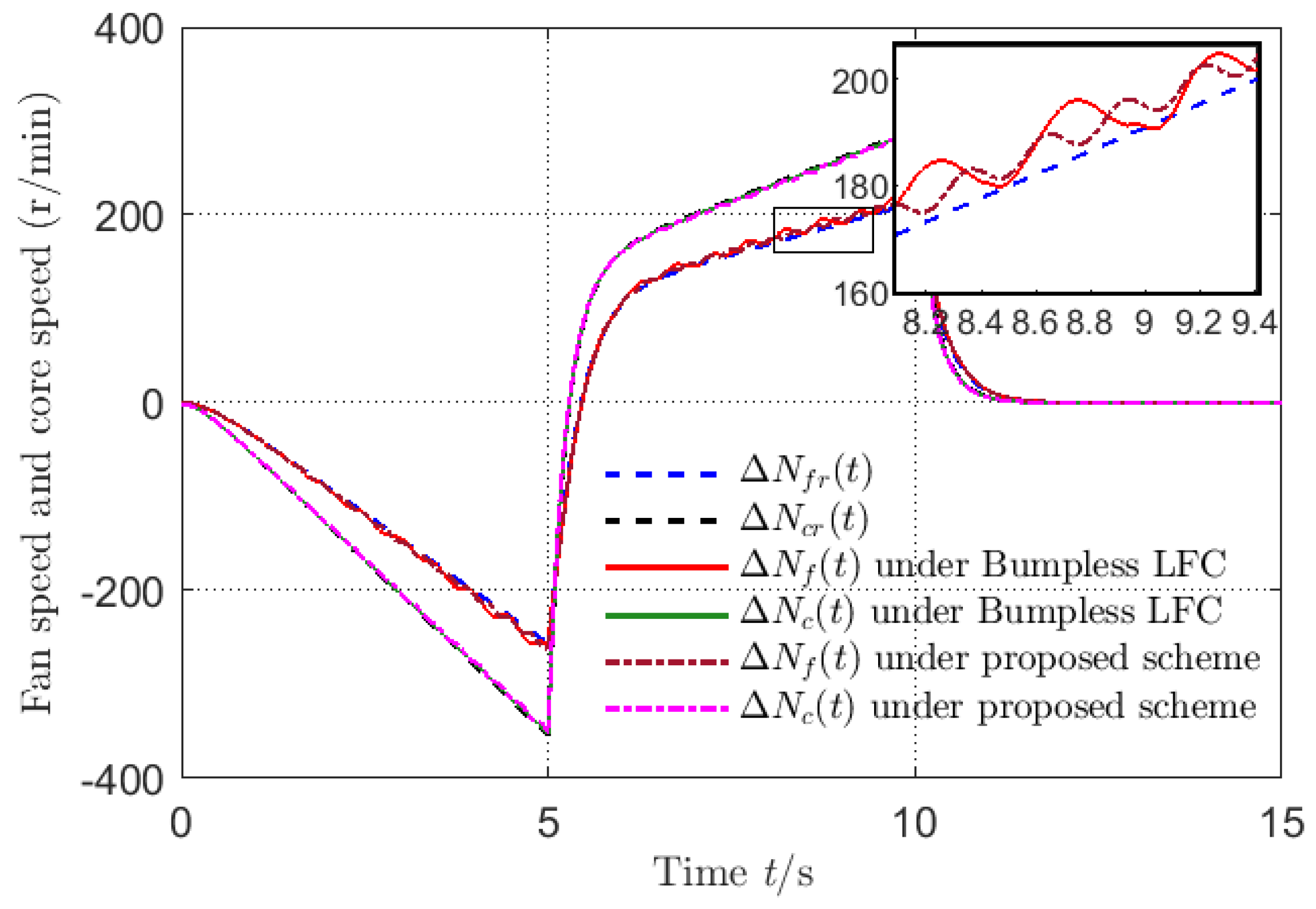
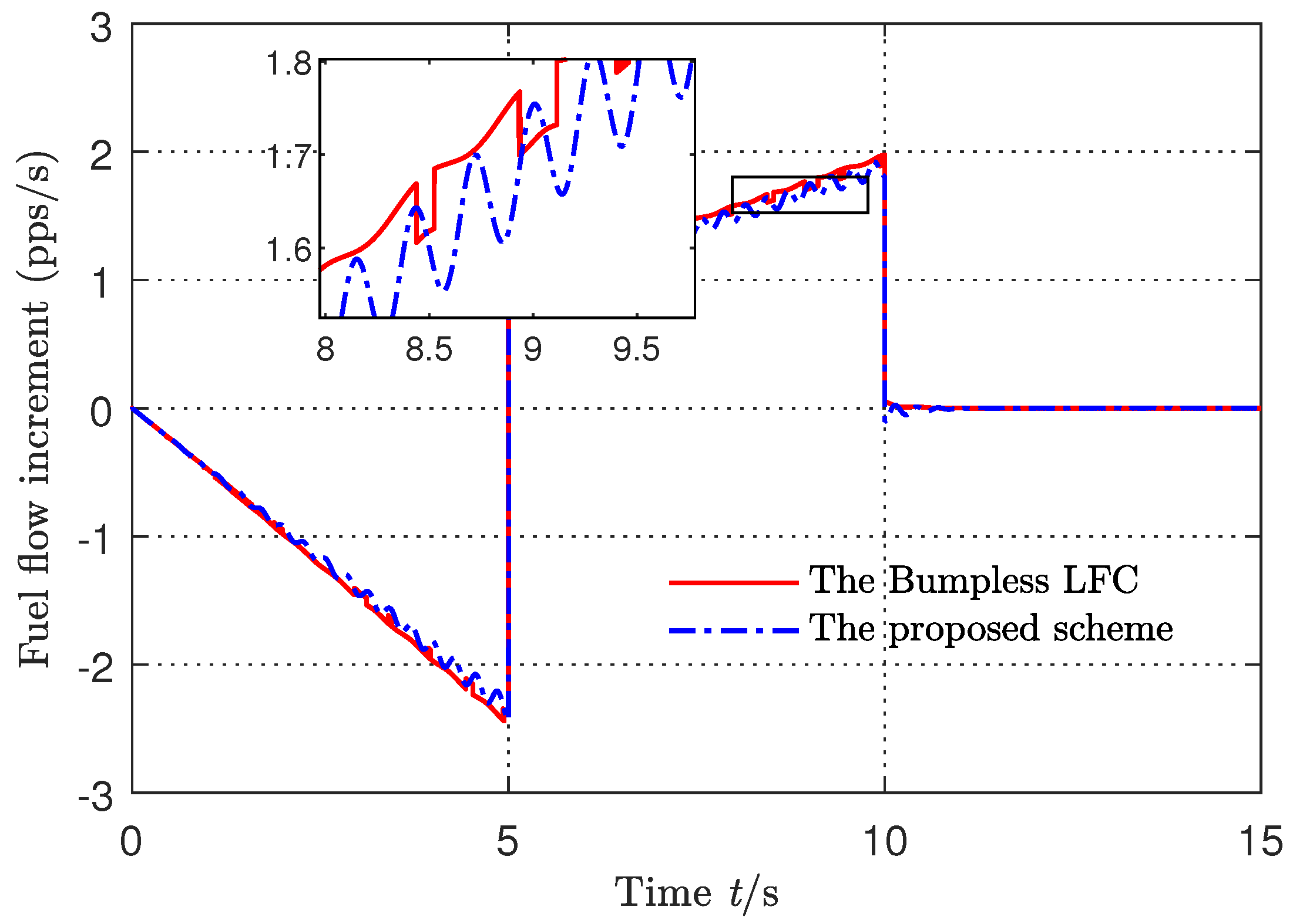
6.1. Example 1: A Turbofan Aeroengine

The switched model of 90K turbofan aeroengine in [30,31] was used to verify the effectiveness of the proposed control scheme. The data in Models (2) and (8) are as follows:

$$\begin{array}{cc}\hfill & A_1=\left[\begin{array}{cc}-3.8557& 1.4467\\ 0.4690& -4.7081\end{array}\right],B_1=\left[\begin{array}{c}230.6739\\ 653.5547\end{array}\right],D_1=\left[\begin{array}{c}1\\ 0.5\end{array}\right],\hfill \\ \hfill & A_2=\left[\begin{array}{cc}-3.7401& 1.4001\\ 0.4752& -4.5586\end{array}\right],B_2=\left[\begin{array}{c}231.5508\\ 657.3084\end{array}\right],D_2=\left[\begin{array}{c}0.8\\ 0.1\end{array}\right],\hfill \\ \hfill & G=\left[\begin{array}{cc}-4.0334& 1.4777\\ 0.5872& -4.6338\end{array}\right],R=\left[\begin{array}{c}225.5204\\ 627.2142\end{array}\right],\omega \left(t\right)=e^{-0.3t}.\hfill \end{array}$$

And the corresponding uncertainties are defined as

$$\begin{array}{cc}\hfill & \Delta A_1=\left[\begin{array}{cc}0.34sin4\pi t& 0\\ 0& 0.4e^{-t}\end{array}\right],\Delta A_2=\left[\begin{array}{cc}0.35cos7\pi t& 0.1e^{-2.2t}\\ 0& 0.23e^{-2.2t}\end{array}\right],\hfill \\ \hfill & \Delta B_1={\left[\begin{array}{cc}0& e^{-3t}\end{array}\right]}^T,\Delta B_2={\left[\begin{array}{cc}0.4& 0\end{array}\right]}^T.\hfill \end{array}$$

The initial condition is $\Delta N_f\left(0\right)=x_{r,1}\left(0\right)=0.5,\Delta N_c\left(0\right)=x_{r,2}\left(0\right)=-2$. Given the bumpless performance indices ${\alpha }_1=0.1$, ${\alpha }_2=1$, by Theorem 1, the coefficients were obtained as

$$\begin{array}{cc}\hfill & K_{1,1}=[3.3836,4.5476],K_{1,2}=\left[\mathrm{3.38274.5479}\right],\hfill \\ \hfill & K_{2,1}={10}^{-3}·[0.0755,0.1160],K_{2,2}={10}^{-4}·[0.1175,-0.6478],\hfill \\ \hfill & K_{3,1}=0.9617,K_{3,2}=0.9564.\hfill \end{array}$$

We designed the RISM parameter $L=[0.02,0.02,1]$, given the $H_{\infty }$ performance index ${\gamma }_1=0.5,{\gamma }_2=0.4$. Using Theorem 2, the parameters of the RISM $K_1,K_2$ were obtained as follows:

$$\begin{array}{cc}\hfill & K_1=[470.1,475.5,5087.1],K_2=\left[\mathrm{333.0552.45084.6}\right],\hfill \end{array}$$

and the matrices $\overline{P},Q,\beta ,{\mu }_i$ are omitted here for brevity. The parameters in the controller (38) were set to ${\lambda }_1={\lambda }_2=10$, ${\eta }_1=2\parallel \overline{e}\left(t\right)\parallel +2\parallel x_r\left(t\right)\parallel +\parallel r\left(t\right)\parallel +4$, ${\eta }_2=0.5{\eta }_1$.

The following two kinds of speed reference inputs were set to be tracked:

$$\begin{array}{c}\hfill r_1\left(t\right)=\left\{\begin{array}{cc}-0.5t,\hfill & 0\le t<5,\hfill \\ 0.2t,\hfill & 5\le t<10,\hfill \\ 0,\hfill & others.\hfill \end{array}\right.\end{array}$$

To compare with the existing control design, the bumpless linear feedback control (LFC) in [31] was repeated in order to be used. The comparing simulation results with the reference input $r\left(t\right)$ are shown in Figure 1, Figure 2 and Figure 3. Figure 1 and Figure 2 show that the tracking performance of the proposed control scheme and the bumpless LFC in [31] were both satisfactory, although there were uncertainties and disturbances. However, the tracking errors under the proposed control scheme were more smaller. Figure 3 shows that the fuel flow control signals did not have big chattering under the switching, and met the bumpless indices without large amplitude jumps. The small jump existed in the control signal of the bumpless LFC scheme in [31], but that in the proposed control scheme was continuous varying.

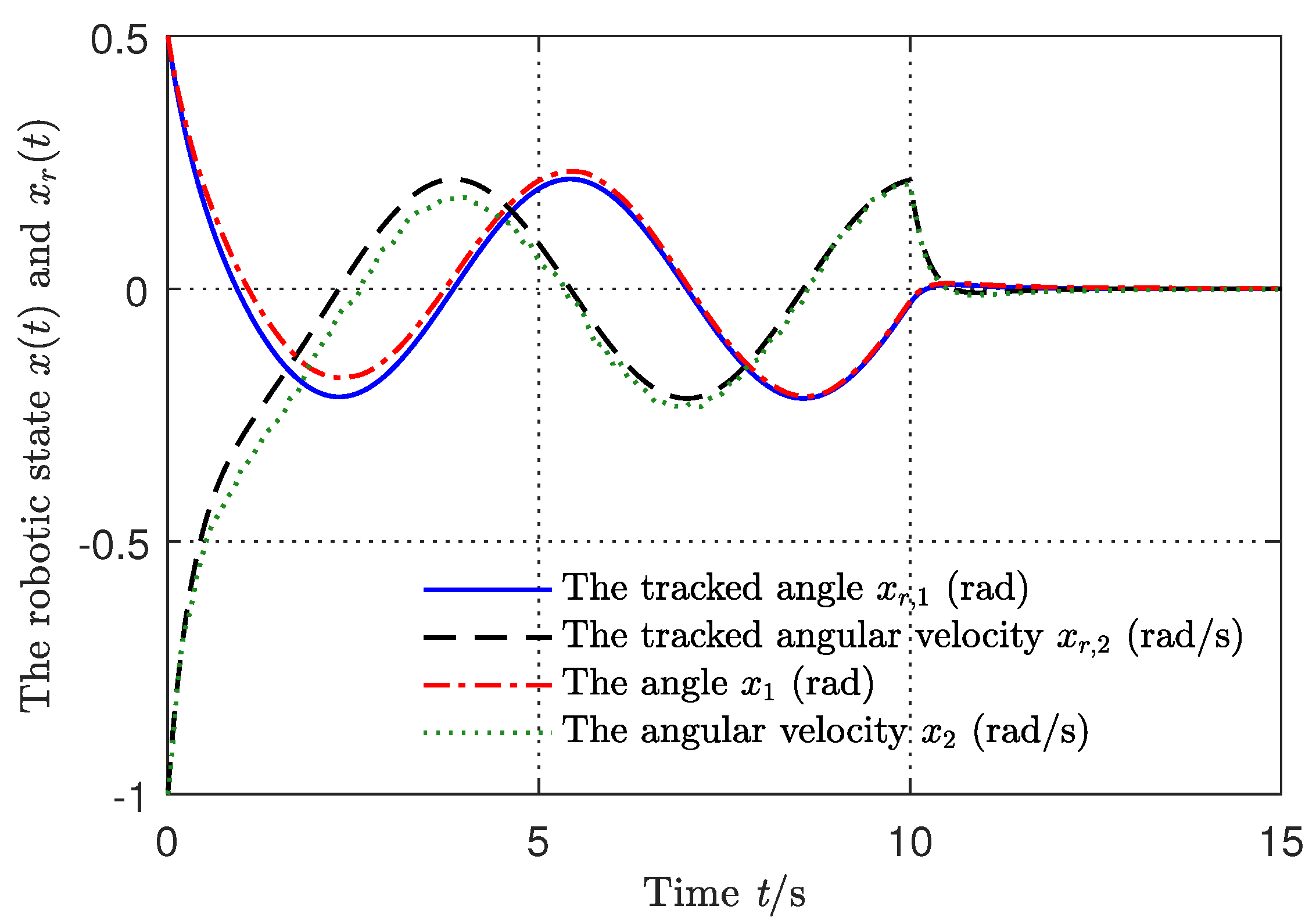
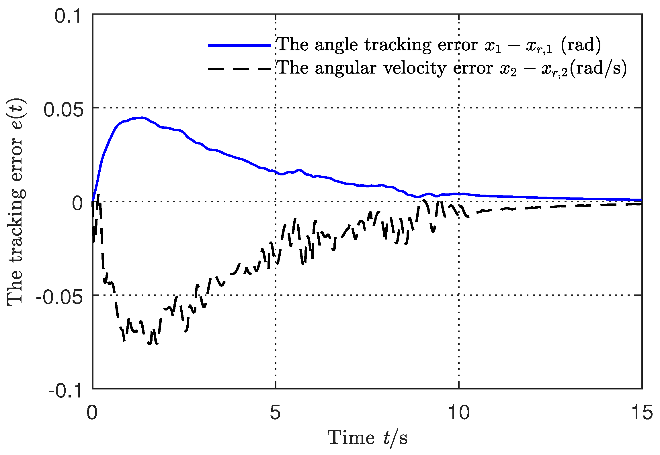
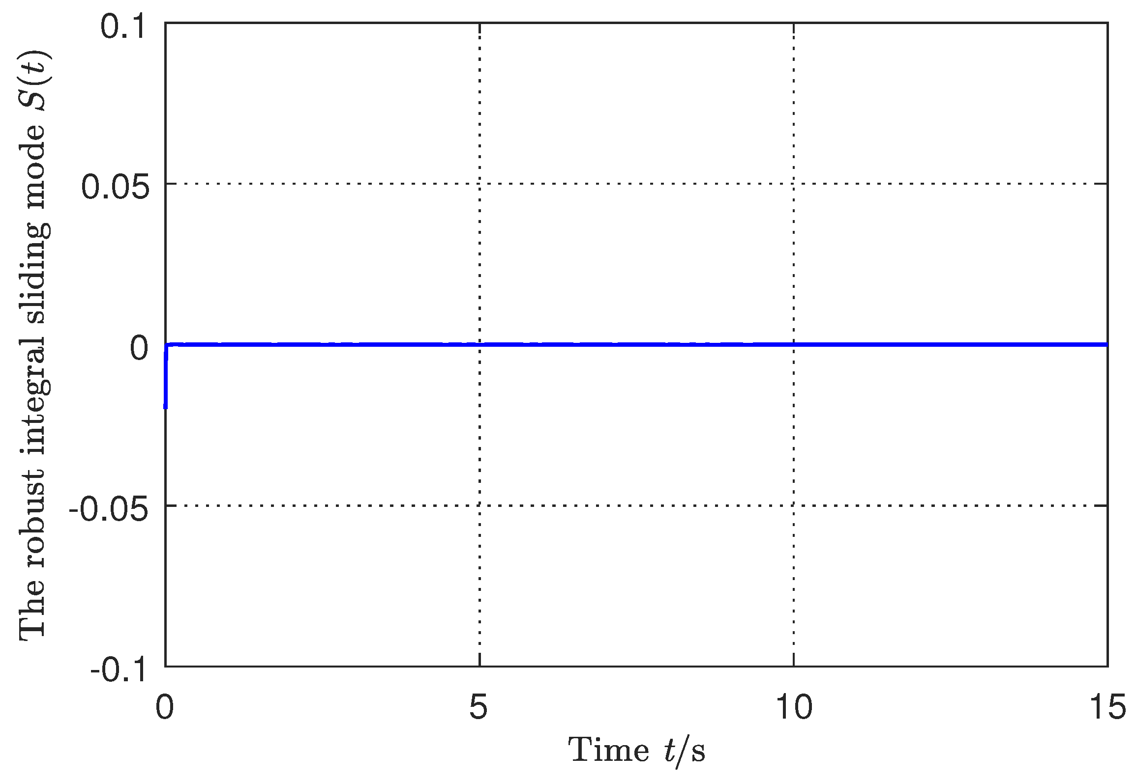
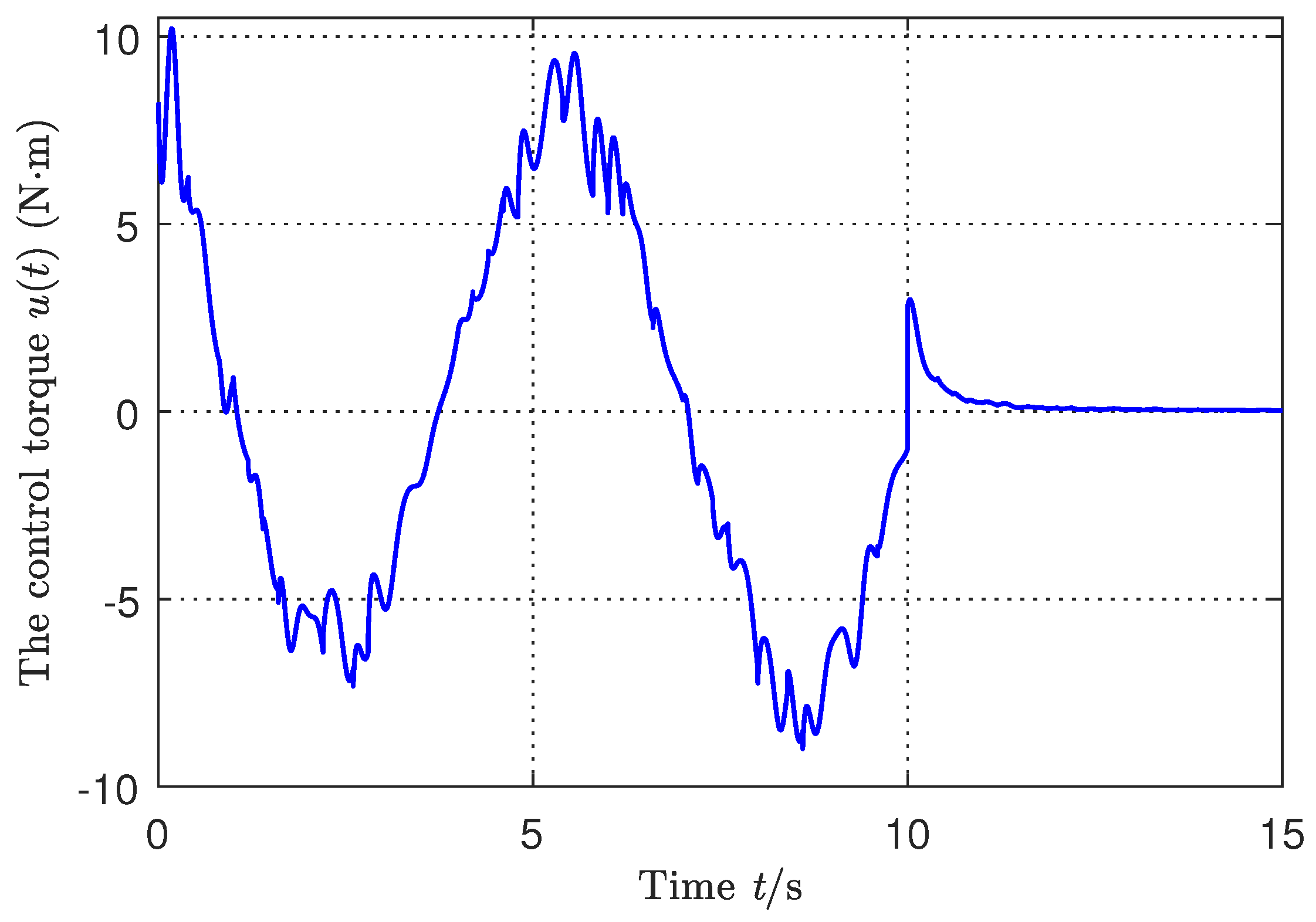
6.2. Example 2: A Manipulator

Consider a one-link robotic manipulator, whose joint angle can only be acquired directly. Its mathematical description is as follows:

$$\begin{array}{cc}{\dot{x}}_1& =x_2,\hfill \\ \hfill {\dot{x}}_2& =-{\displaystyle \frac{mgl}{m{l}^2+J}}cos{x}_1+{\displaystyle \frac{1}{m{l}^2+J}}u\left(t\right)+\varphi \left(t\right),\hfill \\ \hfill y\left(t\right)& =x_1,\hfill \end{array}$$

(40)

where $x_1$ is the joint angle, $x_2$ is the angular velocity, $x={[x_1,x_2]}^T$ is the state vector, m is the mass of the beam, l is the beam length, g represents the gravitational acceleration, and J is the moment of inertia. The control torque is $u\left(t\right)$ and $\varphi \left(t\right)$ indicates the disturbance. It is considered that $z_1=0.5\pi -x_1$, i.e., $z_1$ is the complementary angle of the joint angle with $z_2={\dot{z}}_1=-x_2$, and only the angle $z_1$ can be measured. In this way, by applying the approximation $sin{z}_1\approx z_1$, the mathematical model (40) is transformed into a linear form,

$$\begin{array}{cc}\hfill \dot{z}=& (A+\Delta A)z+Bu\left(t\right)+Dw\left(t\right),y\left(t\right)=Cz,\hfill \end{array}$$

(41)

where $z={[z_1,z_2]}^T$ is the transformed state vector, $w\left(t\right)=\varphi \left(t\right)$ denotes the disturbance, $\Delta z_1$ represents the small angle deviation. The parameter matrices are as follows:

$$\begin{array}{cc}\hfill & A=\left[\begin{array}{cc}0& 1\\ {\displaystyle \frac{mgl}{m{l}^2+J}}& 0\end{array}\right],\Delta A=\left[\begin{array}{cc}0& 1\\ {\displaystyle \frac{\Delta mglcos\Delta z_1}{m{l}^2+J}}& 0\end{array}\right],\hfill \\ \hfill & B={\left[\begin{array}{cc}0& {\displaystyle \frac{-1}{m{l}^2+J}}\end{array}\right]}^T,C={\left[\begin{array}{cc}1& 0\end{array}\right]}^T.\hfill \end{array}$$

When the manipulator grasps different parts in industrial operations, the physical parameters $m,l,J$ will change along with its operation conditions. Therefore, two cases with different loads lead to the switched system with two sets of parameters of System (41),

$$\begin{array}{cc}\hfill & A_1=\left[\begin{array}{cc}0& 1\\ {\displaystyle \frac{m_{1}g{l}_1}{m_1{l}_1^2+J_1}}& 0\end{array}\right],A_2=\left[\begin{array}{cc}0& 1\\ {\displaystyle \frac{m_{2}g{l}_2}{m_2{l}_2^2+J_2}}& 0\end{array}\right],\hfill \\ \hfill & B_1=\left[\begin{array}{c}0\\ {\displaystyle \frac{-1}{m_1{l}_1^2+J_1}}\end{array}\right],B_2=\left[\begin{array}{c}0\\ {\displaystyle \frac{-1}{m_2{l}_2^2+J_2}}\end{array}\right],\hfill \\ \hfill & \Delta A_1=\left[\begin{array}{cc}0& 0\\ {\displaystyle \frac{\Delta mg{l}_{1}cos\Delta z_1}{m_1{l}_1^2+J_1}}& 0\end{array}\right],\Delta A_2=\left[\begin{array}{cc}0& 0\\ {\displaystyle \frac{\Delta mg{l}_{2}cos\Delta z_1}{m_2{l}_2^2+J_2}}& 0\end{array}\right],\hfill \\ \hfill & \Delta B_1={\left[\begin{array}{cc}0& {\displaystyle \frac{1}{m_1{l}_1^2+\Delta J}}\end{array}\right]}^T,\Delta B_2={\left[\begin{array}{cc}0& {\displaystyle \frac{-1}{m_2{l}_2^2+\Delta J}}\end{array}\right]}^T.\hfill \end{array}$$

The physical parameters are given as $m_1=3$ kg, $m_2=3.2$ kg, $l_1=l_2=1$ m, $J_1=0.48$$\mathrm{kg}·{\mathrm{m}}^2$, $J_2=0.52$$\mathrm{kg}·{\mathrm{m}}^2$. It can be proved that $\forall i\in \mathbb{N}$, $(A_i,B_i)$ can be stabilizable and $(A_i,C_i)$ is observable. According to Assumption 2, the uncertainties are decomposed as the following matrices:

$$\begin{array}{cc}\hfill & H_{a,1}=\left[\begin{array}{c}0\\ 1.8\end{array}\right],H_{a,2}=\left[\begin{array}{c}0\\ 1.4\end{array}\right],F_{a,1}=F_{a,2}=cos\Delta z_1,\hfill \\ \hfill & E_{a,1}=E_{a,2}=\left[\begin{array}{cc}0.4& 0\end{array}\right],E_{a,2}=\left[\begin{array}{cc}0.6& 0\end{array}\right],H_{b,1}={\left[\begin{array}{cc}0& 0.6\end{array}\right]}^T,H_{b,2}={\left[\begin{array}{cc}0& -0.4\end{array}\right]}^T,\hfill \\ \hfill & F_{b,1}=F_{b,2}=1,E_{b,1}=E_{b,2}=0.1.\hfill \end{array}$$

The tracked model was set as

$$\begin{array}{c}\hfill G={\left[\begin{array}{cc}0& 1\\ -8& -6\end{array}\right]}^T,R={\left[\begin{array}{c}0\\ 4\end{array}\right]}^T,C_r={\left[\begin{array}{cc}1& 0\end{array}\right]}^T,\end{array}$$

and $D_1=D_2=\left[0.10.1\right]$ are selected with the disturbance $\omega \left(t\right)=e^{-0.3t}$.

According to the parameter design conditions (11)–(13), the parameters are

$$\begin{array}{cc}\hfill & K_{1,1}=[-211.6454,-112.7416],K_{2,1}=[-211.6440,-112.7417],\hfill \\ \hfill & K_{1,2}=[-57.24,-20.88],K_{2,2}=[-61.12,-22.32],\hfill \\ \hfill & K_{1,3}=-13.92,K_{2,3}=-14.88\hfill \end{array}$$

by Theorem 1, with the given performance indices ${\alpha }_1=2,{\alpha }_2=52,{\gamma }_1=0.42,{\gamma }_2=0.38$.

We selected the sliding mode parameter $L=[0.02,0.02,1]$, and designed the common robust integral sliding mode parameter K according to Theorem 2. Moreover, the parameter design conditions (26) were verified. After the above-described calculations, it can be verified that $K=[-29.67,-16.96,1647.84]$ when $\sigma \left(t\right)=1$ and $K=[-33.74,-19.04,1647.83]$ when $\sigma \left(t\right)=2$. These parameters made a RISM based on Theorem 2. We can directly solve the LMIs (26) using the LMI toolbox in Matlab(Version: 2018a; MathWorks, Natick, MA, USA) The matrices $\overline{P}$, Q are found to be

$$\begin{array}{cc}\hfill & \overline{P}=\left[\begin{array}{ccc}0.5725& -1.0257& 0.00012\\ -1.0257& 11.9474& 0.0971\\ 0.00012& 0.0971& 652.15\end{array}\right],Q=\left[\begin{array}{cc}39.2515& 4.6355\\ 4.6355& 2.5931\end{array}\right]\times {10}^5.\hfill \end{array}$$

Thus, the RISM (23) is obtained.

We set the system state initial value as $z\left(t_0\right)={[0.5,-1]}^T$. The sliding mode controller under the arbitrary switching rule can be used according to Theorem 2, for which ${\lambda }_i=10,i=1,2$ were set in the controller (38), and by substituting the system parameter matrices into (39), the practical switched controller can be obtained. The tracked reference signal $r\left(t\right)$ was set as

$$\begin{array}{c}\hfill r_2\left(t\right)=\left\{\begin{array}{cc}-0.5sint,\hfill & 0\le t\le 10,\hfill \\ 0,\hfill & others,\hfill \end{array}\right.\end{array}$$

and the simulation results are shown in Figure 4, Figure 5, Figure 6, Figure 7 and Figure 8.

Figure 4, Figure 5, Figure 6, Figure 7 and Figure 8 display the simulation results of the switched system from which we can observe that under the existence of uncertain parameters, the system state remains on the sliding surface with the arbitrary switching rule from the initial time onward. The control torque signal is shown in Figure 7 and the corresponding switching signal is shown in Figure 8 by the switching rule in Theorem 2. Figure 7 shows that there was not the obvious jump in the control torque signal, which validated the bumpless control performance.

7. Conclusions

Based on the proposed robust integral sliding mode (RISM) design for the switched system with unmatched uncertainty and disturbance, a robust bumpless transfer control scheme of the tracking control is proposed. The controller includes two parts: the RLFC controller and the CSMC controller. The RLFC designed for the uncertain system has not only the robust performance, but also meets the requirements of bumpless transfer indices. The CSMC is designed based on the proposed RISM design, which can suppress the unmatched uncertainty and disturbance. The system state running on the proposed RISM surface has the $H_{\infty }$ robustness to the unmatched uncertainty or disturbance. The combination of the CSMC and the RLFC realizes the requirements of bumpless transfer, unmatched uncertainty suppression at the same time. During control switching, the control signal has no large jump and chattering. Finally, simulation results on the different examples verified the effectiveness of the proposed method.

References

1. Liberzon, D. Switching in Systems and Control; Birkhauser: Boston, MA, USA, 2003. [Google Scholar]
2. Margaliot, M. Stability analysis of switched systems using variational principles: An introduction. Automatica 2006, 42, 2059–2077. [Google Scholar] [CrossRef]
3. Wu, L.; Shi, P.; Su, X. Sliding Mode Control of Uncertain Parameter-Switching Hybrid Systems; John Wiley & Sons: Hoboken, NJ, USA, 2014. [Google Scholar]
4. Wang, Y.; Zhao, J. Neural-network-based event-triggered sliding mode control for networked switched linear systems with the unknown nonlinear disturbance. IEEE Trans. Neural Netw. Learn. Syst. 2023, 34, 3885–3896. [Google Scholar] [CrossRef] [PubMed]
5. Zhang, H.; Zhang, Y.; Zhao, X. Event-triggered adaptive dynamic programming for hierarchical sliding-mode surface-based optimal control of switched nonlinear systems. IEEE Trans. Autom. Sci. Eng. 2024, 21, 4851–4863. [Google Scholar] [CrossRef]
6. Qi, W.; Zhang, N.; Ahn, C.K.; Zong, G. Genetic-algorithm-based sliding mode stabilization for networked switched systems with unreliable channels. IEEE Trans. Control. Netw. Syst. 2024. early access. [Google Scholar] [CrossRef]
7. Wang, T.; Niu, B.; Xu, N.; Zhang, L. ADP-based online compensation hierarchical sliding-mode control for partially unknown switched nonlinear systems with actuator failures. ISA Trans. 2024, in press. [Google Scholar] [CrossRef] [PubMed]
8. Hou, T.; Li, Y.; Lin, Z. Local and global stabilization of switched linear systems with actuator saturation. IEEE Trans. Autom. Control. 2023, 68, 1192–1199. [Google Scholar] [CrossRef]
9. Wang, J.; Wu, J.; Shen, H.; Cao, J.; Rutkowski, L. Fuzzy H control of discrete-time nonlinear Markov jump systems via a novel hybrid reinforcement q-learning method. IEEE Trans. Cybern. 2023, 53, 7380–7391. [Google Scholar] [CrossRef]
10. Wang, J.; Wang, D.; Yan, H.; Shen, H. Composite antidisturbance H control for hidden Markov jump systems with multi-sensor against replay attacks. IEEE Trans. Autom. Control. 2024, 69, 1760–1766. [Google Scholar] [CrossRef]
11. Wang, Z.; Sun, J.; Chen, J. Stability analysis of switched nonlinear systems with multiple time-varying delays. IEEE Trans. Syst. Man Cybern. Syst. 2022, 52, 3947–3956. [Google Scholar] [CrossRef]
12. Jiang, B.; Karimi, H.R.; Zhang, X.; Wu, Z. Adaptive neural-network-based sliding mode control of switching distributed delay systems with Markov jump parameters. Neural Netw. 2023, 165, 846–859. [Google Scholar] [CrossRef]
13. Wang, X.; Ma, Y. Adaptive non-fragile sliding mode control for switched semi-Markov jump system with time-delay and attack via reduced-order method. Appl. Math. Comput. 2023, 440, 127670. [Google Scholar] [CrossRef]
14. Fei, Z.; Wu, Z.; Zhao, X.; Zong, G.; Lin-Shi, X. Reachability-guaranteed sliding mode control for asynchronously switched uncertain systems. IEEE Trans. Autom. Control. 2024. early access. [Google Scholar] [CrossRef]
15. Utkin, V.I.; Shi, J. Integral sliding mode in systems operating under uncertainty conditions. In Proceedings of the 35th IEEE Conference on Decision and Control, Kobe, Japan, 13 December 1996; pp. 4591–4596. [Google Scholar] [CrossRef]
16. Cao, W.J.; Xu, J.X. Nonlinear integral-type sliding surface for both matched and unmatched uncertain systems. IEEE Trans. Autom. Control. 2004, 49, 1355–1360. [Google Scholar] [CrossRef]
17. Kchaou, M.; Al Ahmadi, S. Robust H control for nonlinear uncertain switched descriptor systems with time delay and nonlinear input: A sliding mode approach. Complexity 2017, 2017, 1027909. [Google Scholar] [CrossRef]
18. Chen, H.; Lim, C.C.; Shi, P. Robust H-based control for uncertain stochastic fuzzy switched time-delay systems via integral sliding mode strategy. IEEE Trans. Fuzzy Syst. 2022, 30, 382–396. [Google Scholar] [CrossRef]
19. Song, L.; Tong, S. Observer-based integral sliding mode control with switching gains for fuzzy impulsive stochastic systems. IEEE Trans. Fuzzy Syst. 2024, 32, 1078–1086. [Google Scholar] [CrossRef]
20. Niu, S.; Chen, W.H.; Lu, X.; Xu, W. Integral sliding mode control design for uncertain impulsive systems with delayed impulses. J. Frankl. Inst. 2023, 360, 13537–13573. [Google Scholar] [CrossRef]
21. Ferrara, A.; Incremona, G.P.; Sangiovanni, B. Tracking control via switched integral sliding mode with application to robot manipulators. Control. Eng. Pract. 2019, 90, 257–266. [Google Scholar] [CrossRef]
22. Qi, W.; Gao, X.; Ahn, C.K.; Cao, J.; Cheng, J. Fuzzy integral sliding-mode control for nonlinear semi-Markovian switching systems with application. IEEE Trans. Syst. Man Cybern. Syst. 2022, 52, 1674–1683. [Google Scholar] [CrossRef]
23. Zhang, X.; Xiao, L.; Li, H. Robust control for switched systems with unmatched uncertainties based on switched robust integral sliding mode. IEEE Access 2020, 8, 138396–138405. [Google Scholar] [CrossRef]
24. Zhang, X. Robust integral sliding mode control for uncertain switched systems under arbitrary switching rules. Nonlinear Anal. Hybrid Syst. 2020, 37, 100900. [Google Scholar] [CrossRef]
25. Kao, Y.; Liu, X.; Song, M.; Zhao, L.; Zhang, Q. Nonfragile-observer-based integral sliding mode control for a class of uncertain switched hyperbolic systems. IEEE Trans. Autom. Control. 2022, 68, 5059–5066. [Google Scholar] [CrossRef]
26. Wang, C.; Li, R.; Su, X.; Shi, P. Output feedback sliding mode control of Markovian jump systems and its application to switched boost converter. IEEE Trans. Circuits Syst. Regul. Pap. 2021, 68, 5134–5144. [Google Scholar] [CrossRef]
27. Zhang, X.; Xiao, L.; Tan, R.; Liu, W. Bumpless Transfer Control Design of Continuous Integral Sliding Mode Switching Controller for Turbofan Aeroengine. In Proceedings of the 2022 IEEE 17th International Conference on Control and Automation (ICCA), Naples, Italy, 27–30 June 2022; pp. 868–873. [Google Scholar] [CrossRef]
28. Wang, Y.; Xie, L.; de Souza, C.E. Robust control of a class of uncertain nonlinear systems. Syst. Control. Lett. 1992, 19, 139–149. [Google Scholar] [CrossRef]
29. Shi, J.; Zhao, J. State bumpless transfer control for a class of switched descriptor systems. IEEE Trans. Circuits Syst. Regul. Pap. 2021, 68, 3846–3856. [Google Scholar] [CrossRef]
30. Richter, H. Advanced Control of Turbofan Engines; Springer: New York, NY, USA, 2014. [Google Scholar]
31. Zhao, Y.; Fu, J.; Zhao, J. Bumpless transfer control for switched systems and its application to aeroengines. ACTA Autom. Sin. 2020, 46, 2165–2176. [Google Scholar] [CrossRef]
Figure 1. The aeroengine state tracking curves along the reference r ( t ) .
Mathematics 12 03504 g001
Figure 2. The aeroengine state tracking error curves.
Mathematics 12 03504 g002
Figure 3. The control signals of the fuel flow increment curves.
Mathematics 12 03504 g003
Figure 4. The angle and angular velocity stabilization curves.
Mathematics 12 03504 g004
Figure 5. The state observation error.
Mathematics 12 03504 g005
Figure 6. The RISM signal.
Mathematics 12 03504 g006
Figure 7. The control torque curve.
Mathematics 12 03504 g007
Figure 8. The switching signal.
Mathematics 12 03504 g008
Disclaimer/Publisher’s Note: The statements, opinions and data contained in all publications are solely those of the individual author(s) and contributor(s) and not of MDPI and/or the editor(s). MDPI and/or the editor(s) disclaim responsibility for any injury to people or property resulting from any ideas, methods, instructions or products referred to in the content.