Optimizing HX-Group Compositions Using C++: A Computational Approach to Dihedral Group Hyperstructures

Abstract

The HX-groups represent a generalization of the group notion. The Chinese mathematicians Mi Honghai and Li Honxing analyzed this theory. Starting with a group $(G,·)$, they constructed another group $(\mathcal{G},\ast )\subset {\mathcal{P}}^{\ast }\left(G\right)$, where ${\mathcal{P}}^{\ast }\left(G\right)$ is the set of non-empty subsets of G. The hypercomposition “$\ast$” is thus defined for any A, B from G, $A\ast B=\{a·b|a\in A,b\in B\}.$ In this article, we consider a particular group, G, to be the dihedral group $D_n,n$ is a natural number, greater than 3, and we analyze the HX-groups with the dihedral group $D_n$ as a support. The HX-groups were studied algebraically, but the novelty of this article is that it is a computer analysis of the HX-groups by creating a program in $C++$. This code aims to improve the calculation time regarding the composition of the HX-groups. In the first part of the paper, we present some results from the hypergroup theory and HX-groups. We create another hyperstructure formed by reuniting all the HX-groups associated with a dihedral group $D_n$ as a support for a natural fixed number n. In the second part, we present the $C++$ code created in the Microsoft Visual Studio program, and we provide concrete examples of the program’s application. We created this program because the code aims to improve the calculation time regarding the composition of HX-groups.

1. Introduction

Hypergroup theory represents a generalization of classical algebraic structures. F. Marty noticed that the quotient group’s elements are sets, and he introduced the concept of a hypergroup in 1934 [1]. Over time, the theory of hypergroups has developed greatly from a theoretical point of view. It has applications in numerous fields, such as geometry, topology, cryptography, code theory, graphs, hypergraphs, automata theory, fuzzy degree, probability, etc. [2,3,4,5,6,7,8]. Starting with a non-empty set H and the hyperoperation $“\circ ”:H\times H\to {\mathcal{P}}^{\ast }\left(H\right)$, where ${\mathcal{P}}^{\ast }\left(H\right)$ represents the collection of all non-empty subsets of H, we obtained a semihypergroup if and only if the hyperoperation satisfies the associativity relation, i.e., $(a\circ b)\circ c=a\circ \left(b\circ c\right)$, for any a, b, c $\in H^3$. Also, $\left(H,\circ \right)$ is a quasihypergroup if and only if the hyperoperation satisfies the reproducibility relation, i.e., $H\circ a=a\circ H=H$, for any $a\in H$. We say that $\left(H,\circ \right)$ is a hypergroup if and only if “$\circ$” satisfies the associativity and reproducibility relation. In hypergroup theory, we can compute two sets in the following way: for any A, B sets from H, $A\circ B=A\circ B=\cup \{a\circ b/a\in A,b\in B\}.$ In 1985, three Chinese mathematicians, HongXing Li, QinZhi Duan, and PeizHuang, used the term “hypergroup” [9]. Later, Li renamed the concept with the term HX-groups [10]. Zhenliang studied the properties of HX-groups [11], and, recently, the interest in this concept has increased. Corsini studied the hypergroups associated with $\mathbb{Z}/n\mathbb{Z}$, the Chinese hypergroupoid of an HX-group, and found conditions such that the Chinese hypergroupoid becomes a hypergroup; see [12,13,14]. Cristea established a link between HX-groups and hypergroups [15]. Sonea determined the HX-groups with dihedral group $D_n$ as a support [16], created a new commutative hyperstructure that considered the union of all the HX-groups [17], and studied the NeutroHX-groups [18]. Also, Mousavi, Jafarpour, and Cristea studied the HX-Polygroups [19]. This article is divided into three sections. The first section refers to the introductory notions from the theory of HX-groups and the theory of hypergroups. Also, a new hyperstructure ${\mathcal{G}}_n$ formed by the union of all the HX-groups associated with the dihedral group $D_n$ for a fixed natural number n is presented [17]. Until now, HX-groups have been analyzed only from an algebraic point of view. In the second part of the article, a computational approach to HX-groups is presented using code in the $C++$ programming language. This code facilitates the calculation time regarding the composition of HX-groups, and the third section refers to the connection between HX-groups and graph theory.

2. The Construction of the Hyperstructure ${\mathcal{G}}_{\mathit{n}}$

In this section, we will present the construction of the hyperstructure ${\mathcal{G}}_n$. We consider a new hyperstructure formed by the union of all HX-groups with the dihedral group $D_n$ as support for a fixed natural number $n>3$ [17]. In what follows, we recall the basic notions of HX-groups.

Definition 1

([10]). Let $(G,·)$ be a group and $\mathcal{G}\subset$${\mathcal{P}}^{\ast }\left(G\right)$, where ${\mathcal{P}}^{\ast }\left(G\right)$ is the set of non-empty subsets of $G$. An HX-group is a non-empty subset H of ${\mathcal{P}}^{\ast }\left(G\right)$, which is a group with respect to the operation “*” defined by

$$\forall A,B\in \mathcal{G},A\ast B=\{a·b|a\in A,b\in B\}.$$

(1)

We say that $\mathcal{G}$ has group G as support.

The HX-groups with the dihedral group $D_n$ as support denoted by ${\mathcal{G}}_{p_1}^{q_1}$ are determined [16].

Theorem 1

([16]). For $n=p_1{q}_1,$ $p_1,q_1\in {\mathbb{N}}^{\ast }$, the $({\mathcal{G}}_{p_1}^{q_1},\ast )$ is an HX-group associated with the dihedral group $D_n$ with elements

$$\begin{array}{ccc}\hfill A_i& =& \{{\rho }^i,{\rho }^{q_1+i},{\rho }^{2q_1+i},\dots ,{\rho }^{(p_1-1)q_1+i}\};\hfill \\ \hfill A_{q_1+i}& =& \{{\rho }^i\sigma ,{\rho }^{q_1+i}\sigma ,{\rho }^{2q_1+i}\sigma ,\dots ,{\rho }^{(p_1-1)q_1+i}\sigma \};\hfill \end{array}$$

where $i\in \{0,1,\dots ,q_1-1\}$.

Proposition 1.

The $<{\rho }^q>$ is a normal subgroup in $D_n$, where $n=pq$, p, q are natural numbers.

Proof. 

In what follows, we will recall the definition of a normal subgroup, which we will apply [20] in the demonstration. Let $\left(G,·\right)$ be a group and H a subgroup of G. For any x in G, H is a normal subgroup in G if and only if $xH=Hx$. In this case,

$$H= <{\rho }^q> =\{e,{\rho }^q,q^{2q},\dots ,q^{(p-1)q}\}.$$

Therefore, the elements in H are of the form ${\rho }^{kq}$, $k\in \{0,1,\dots ,p-1\}$. We have to show that $x{\rho }^{kq}{x}^{-1}\in H$ for any $x\in D_n$ and $k\in \{0,1,\dots ,p-1\}.$ For $x={\rho }^t,t\in \{0,1,\dots ,n-1\}$, we obtain

$$xh{x}^{-1}={\rho }^t{\rho }^{kq}{\left({\rho }^t\right)}^{-1}={\rho }^{t+kq+n-t}={\rho }^{n+kq}={\rho }^n{\rho }^{kq}=e{\rho }^{kq}={\rho }^{kq}\in H.$$

For $x={\rho }^t\sigma$,

$$\begin{array}{ccc}\hfill xh{x}^{-1}& =& {\rho }^t\sigma {\rho }^{kq}{\left({\rho }^t\sigma \right)}^{-1}={\rho }^t\sigma {\rho }^{kq}{\rho }^t\sigma ={\rho }^t\sigma {\rho }^{kq+t}\sigma \hfill \\ & =& {\rho }^t\sigma \sigma {\rho }^{n-(kq+t)}={\rho }^{t}e{\rho }^{n-(kq+t)}={\rho }^{t+n-(kq+t)}\hfill \\ & =& {\rho }^{n-kq}={\rho }^{(p-k)q}\in H.\hfill \end{array}$$

In conclusion, $<{\rho }^q>$ is a normal subgroup in the dihedral group $D_n.$    □

Proposition 2.

The HX-group obtained previously represents the quotien group $G_p^q={\displaystyle \frac{D_n}{<{\rho }^q>}}$ for $n=pq.$

Proof. 

We proved before that $<{\rho }^q>$ is a normal subgroup in $D_n$, so

$${\displaystyle \frac{D_n}{<{\rho }^q>}}=\{x<{\rho }^q>/x\in D_n\}.$$

For $x={\rho }^t,t\in \{0,1,\dots ,n-1\}$, we obtain

$${\rho }^t<{\rho }^q> ={\rho }^t·\{e,{\rho }^q,q^{2q},\dots ,q^{(p-1)q}\}=\{{\rho }^t,{\rho }^{t+q},\dots ,{\rho }^{t+\left(p-1\right)q}\}=A_t,$$

where $A_t$ is defined by Theorem 1.

For $x={\rho }^t\sigma$, $t\in \{0,1,\dots ,n-1\}$, we have

$$\begin{array}{ccc}\hfill {\rho }^t\sigma & <& {\rho }^q> ={\rho }^t\sigma ·\{e,{\rho }^q,q^{2q},\dots ,q^{(p-1)q}\}=\{{\rho }^t\sigma ,{\rho }^t\sigma {\rho }^q,{\rho }^t\sigma q^{2q},\dots ,{\rho }^t\sigma q^{(p-1)q}\}\hfill \\ & =& \{{\rho }^t\sigma ,{\rho }^t{\rho }^{n-q}\sigma ,{\rho }^t{\rho }^{n-2q}\sigma ,\dots ,{\rho }^t{\rho }^{n-\left(p-1\right)q}\sigma \}\hfill \\ & =& \{{\rho }^t\sigma ,{\rho }^{t+\left(p-1\right)q}\sigma ,{\rho }^{t+\left(p-2\right)q}\sigma ,\dots ,{\rho }^{t+q}\sigma \}\hfill \\ & =& \{{\rho }^t\sigma ,{\rho }^{t+q}\sigma ,\dots ,{\rho }^{t+\left(p-2\right)q}\sigma ,{\rho }^{t+\left(p-1\right)q}\sigma \}=A_{q+t},\hfill \end{array}$$

where $A_{q+t}$, is defined by Theorem 1. Therefore, we can conclude that ${\displaystyle \frac{D_n}{<{\rho }^q>}}=G_p^q.$    □

After that, we took into consideration the union of all HX-groups associated with a dihedral group $D_n$ as support, and we obtained a new hyperstructure defined in [17].

$${\mathcal{G}}_n=\left\{{\mathcal{G}}_{p_1}^{q_1}|HX-\mathrm{groups}\mathrm{for}\mathrm{any}{p}_1,q_1\in {\mathbb{N}}^{\ast }\mathrm{such}\mathrm{that}n=p_1{q}_1\right\}$$

is the set of all HX-groups. We define the hyperoperation $“\circ ”:$${\mathcal{G}}_n\times {\mathcal{G}}_n\to P^{\ast }\left({\mathcal{G}}_n\right)$; thus,

$$\begin{array}{ccc}\hfill {\mathcal{G}}_{p_1}^{q_1}\circ {\mathcal{G}}_{p_2}^{q_2}& =& \bigcup _{0\le s\le 2p_1-1}\left(\bigcup _{0\le t\le 2p_2-1}{C}_{s,t}\right),\hfill \\ \hfill C_{s,t}& =& X_s^{q_1}\ast Y_t^{q_2};X_s^{q_1}\in {\mathcal{G}}_{p_1}^{q_1},Y_t^{q_2}\in {\mathcal{G}}_{p_2}^{q_2}\hfill \\ \hfill n& =& p_1{q}_1=p_2{q}_2,p_1,q_1,p_2,q_2\in {\mathbb{N}}^{\ast }.\hfill \end{array}$$

We analyzed the hyperstructure $\left({\mathcal{G}}_4,\circ \right)$ and obtained some results; see [17].

Proposition 3.

The hyperstructure $\left({\mathcal{G}}_4,\circ \right)$ is a commutative structure where

$${\mathcal{G}}_4=\left\{{\mathcal{G}}_{p_1}^{q_1}|HX-\mathrm{groups},\mathrm{for}\mathrm{any}{p}_1,q_1\in {\mathbb{N}}^{\ast }\mathrm{such}\mathrm{that}4=p_1{q}_1\right\}.$$

Remark 1.

The elements of the hyperstructure $\left({\mathcal{G}}_4,\circ \right)$ satisfy the following equality

$${\mathcal{G}}_{p_1}^{q_1}\circ {\mathcal{G}}_{p_2}^{q_2}={\mathcal{G}}_{p_2}^{q_2}\circ {\mathcal{G}}_{p_1}^{q_1}={\mathcal{G}}_{gcd\{p_1,p_2\}}^{lcm\{q_1,q_2\}},$$

(2)

for any $p_1$, $q_1$,$q_2$,$p_2\in {\mathbb{N}}^{\ast }$ such that $4=p_1{q}_1=p_2{q}_2.$

lcm$\{q_1,q_2\}$ represents the least common multiple of numbers $q_1,q_2$, and gcd$\{p_1,p_2\}$ represent the greatest common divisors of $p_1,p_2$.

Proposition 4.

The hyperstructure $\left({\mathcal{G}}_4,\circ \right)$ is a semihypergroup, but not a quasihypergroup.

Now, we present the connection between the number of cyclic subgroups and the cardinality of ${\mathcal{G}}_n.$

Remark 2.

The cyclic subgroups of the dihedral group $D_n$ are $<\sigma >,<\rho \sigma >,\dots ,<{\rho }^{n-1}\sigma >$, and $<{\rho }^d>$, where d is a divisor of n. So, the number of all cyclic subgroups is $n+\tau \left(n\right)$, where $\tau \left(n\right)=\left({\alpha }_1+1\right)\left({\alpha }_2+1\right)\dots \left({\alpha }_k+1\right)$, $n=p_1^{{\alpha }_1}{p}_2^{{\alpha }_2}\dots p_k^{{\alpha }_k}.$

Proposition 5.

The cardinality of the hyperstructure ${\mathcal{G}}_n$ is equal to the number of normal subgroups of a dihedral group $D_n$. 

Proof. 

According to Proposition 1 and Remark 2, we can state that the normal subgroups of the dihedral group $D_n$ are $<{\rho }^d>,$ where d is a divisor of n. Also, the construction of the hyperstructure ${\mathcal{G}}_n$ implies that the $|{\mathcal{G}}_n|=\tau \left(n\right)$, where $\tau \left(n\right)=\left({\alpha }_1+1\right)\left({\alpha }_2+1\right)\dots \left({\alpha }_k+1\right)$, $n=p_1^{{\alpha }_1}{p}_2^{{\alpha }_2}\dots p_k^{{\alpha }_k}.$ The conclusion is immediate.     □

Example 1.

We determine the composition between the HX-groups ${\mathcal{G}}_1^4$ and ${\mathcal{G}}_2^2$, where

$$\begin{array}{ccc}\hfill {\mathcal{G}}_2^2& =& \{\{e,{\rho }^2\},\{\rho ,{\rho }^3\},\{\sigma ,{\rho }^2\sigma \},\{\rho \sigma ,{\rho }^3\sigma \}\};\hfill \\ \hfill {\mathcal{G}}_1^4& =& \{\{e,\rho ,{\rho }^2,{\rho }^3\},\{\sigma ,\rho \sigma ,{\rho }^2\sigma ,{\rho }^3\sigma \}\}.\hfill \end{array}$$

Therefore,

$${\mathcal{G}}_1^4\ast {\mathcal{G}}_2^2=\{C_{0,0},C_{0,1},C_{0,2},C_{0,3},C_{1,0},C_{1,1},C_{1,2},C_{1,3}\},$$

and the sets $X_s^{q_1}$,$Y_t^{q_2}$, where $s\in \{0,1\},t\in \{0,1,2,3\},$ $q_1=4,$ $q_2=2$, are

$$\begin{array}{ccc}\hfill X_0^4& =& \{e,\rho ,{\rho }^2,{\rho }^3\},X_1^4=\{\sigma ,\rho \sigma ,{\rho }^2\sigma ,{\rho }^3\sigma \},\hfill \\ \hfill Y_0^2& =& \{e,{\rho }^2\},Y_1^2=\{\rho ,{\rho }^3\},Y_2^2=\{\sigma ,{\rho }^2\sigma \},Y_3^2=\{\rho \sigma ,{\rho }^3\sigma \}.\hfill \end{array}$$

In the following, we calculate the elements $C_{i,j}$, $i\in \{0,1\}$,  $j\in \{0,1,2,3\}$.

$$\begin{array}{ccc}\hfill C_{0,0}& =& X_0^4\ast Y_0^2=\{e,\rho ,{\rho }^2,{\rho }^3\}\ast \{e,{\rho }^2\}=e·e\cup e·{\rho }^2\cup \rho ·e\cup \hfill \\ & & \cup \rho ·{\rho }^2\cup {\rho }^2·e\cup {\rho }^2·{\rho }^2\cup {\rho }^3·e\cup {\rho }^3·{\rho }^3\hfill \\ & =& \{e,\rho ,{\rho }^2,{\rho }^3\}=X_0^4;\hfill \\ \hfill C_{0,1}& =& X_0^4\ast Y_1^2=\{e,\rho ,{\rho }^2,{\rho }^3\}\ast \{\rho ,{\rho }^3\}=\hfill \\ & =& e·\rho \cup e·{\rho }^3\cup \rho ·\rho \cup \rho ·{\rho }^3\cup \hfill \\ & & \cup {\rho }^2·\rho \cup {\rho }^2·{\rho }^3\cup {\rho }^3·\rho \cup {\rho }^3·{\rho }^3.\hfill \\ & =& \{e,\rho ,{\rho }^2,{\rho }^3\}=X_0^4\hfill \\ \hfill C_{0,2}& =& X_0^4\ast Y_2^2=\{e,\rho ,{\rho }^2,{\rho }^3\}\ast \{\sigma ,{\rho }^2\sigma \}=\hfill \\ & =& \{\sigma ,\rho \sigma ,{\rho }^2\sigma ,{\rho }^3\sigma \}=X_1^4.\hfill \\ \hfill C_{0,3}& =& X_0^4\ast Y_3^2=\{e,\rho ,{\rho }^2,{\rho }^3\}\ast \{\rho \sigma ,{\rho }^3\sigma \}=X_1^4.\hfill \end{array}$$

Similarly, we obtain

$$C_{1,0}=X_1^4\ast Y_0^2=X_1^4,C_{1,1}=X_1^4\ast Y_1^2=X_1^4,C_{1,2}=X_1^4\ast Y_1^2=X_0^4,C_{1,3}=X_1^4\ast Y_1^3=X_0^4.$$

So, we have

$${\mathcal{G}}_1^4\circ {\mathcal{G}}_2^2={\mathcal{G}}_1^4.$$

Remark 3.

The calculation time for composing two HX-groups can be quite high. This represents the starting point of the idea of creating code in the $\mathit{C}++$ programming language because we can improve the calculation time and analyze higher-order HX-groups.

3. Materials and Methods

Implementing $\mathit{C}++$ Code into Microsoft Visual Studio 2022

This section will present the code in the $\mathit{C}++$ programming language, created in Microsoft Visual Studio 2022. The code describes the HX-groups associated with the dihedral group $D_n$ and their composition. Creating such a program was needed to improve the calculation time for composing the HX-groups. The composition problem can become quite complex, as observed in the works [17,18]. The input data will be n (the order of the dihedral group $D_n$), and the divisors $p_1,q_1,p_2,q_2$ so that $n=p_1{q}_1=p_2{q}_2$. In the program, we identify the HX-group ${\mathcal{G}}_{p_1}^{q_1}$ with $G(p_1,q_1)$; the elements of ${\mathcal{G}}_{p_1}^{q_1}$ formed a matrix and are noted with $a\left[i\right]\left[j\right]$, and similarly the elements of ${\mathcal{G}}_{p_2}^{q_2}$ are noted through $b\left[i\right]\left[j\right]$. We identify the elements of the dihedral group with natural numbers. So, we consider the function $f:(D_n,·)\to (\mathbb{N},+)$ as follows:

$$\begin{array}{ccc}\hfill f\left({\rho }^k\right)& =& k,\hfill \\ \hfill f\left({\rho }^k\sigma \right)& =& n+k,\hfill \end{array}$$

(3)

where $k\in \{0,1,\dots ,n-1\}.$ For a fixed natural number n, we consider the restriction of function $f,$ so $f:(D_n,·)\to (\{0,1,\dots ,2n-1\},+).$ In these conditions, we can state the following:

Proposition 6.

For a fixed natural number n, the function $f:(D_n,·)\to (\{0,1,\dots ,2n-1\},+)$

$$\begin{array}{ccc}\hfill f\left({\rho }^k\right)& =& k,\hfill \\ \hfill f\left({\rho }^k\sigma \right)& =& n+k,\hfill \end{array}$$

(4)

is a bijective function.

Proof. 

The injectivity results immediately because, for any x,$y\in D_n$ such that $f\left(x\right)=f\left(y\right)$, it implies $x=y$. The elements from $D_n$ have the form ${\rho }^k$ or ${\rho }^k\sigma$. As we can see, $f\left({\rho }^k\right)\ne f\left({\rho }^k\sigma \right)$ for any $k\in \{0,1,\dots ,n-1\}.$ So, to have the equality $f\left(x\right)=f\left(y\right)$ means that $x={\rho }^k$, $y={\rho }^p$, k, $p\in \{0,1,\dots ,n-1\},$ or $x={\rho }^k\sigma$, $y={\rho }^p\sigma .$ In both cases, it results that $p=k$; this means that $x=y.$ To study the surjectivity, we have to prove that, for any element k from $\{0,1,\dots ,2n-1\}$, there is $x\in D_n$ such that $f\left(x\right)=k$. For $k\in \{0,1,\dots ,n-1\},$ we consider $x={\rho }^k$, and, for $k\ge n,$ we consider $x={\rho }^{k-n}\sigma$. In conclusion, f is a bijective function.    □

To determine the composition of groups ${\mathcal{G}}_{p_1}^{q_1}\circ {\mathcal{G}}_{p_2}^{q_2}$, where $n=p_1{q}_1=p_2{q}_2$, we have four cases. We denote by ⊕ the composition law created in the program mentioned above, and we provide the composition rules in each case.

Case 1. We compute the elements that have the form ${\rho }^k$ with ${\rho }^p$, for any k, $p\in \{0,1,\dots ,n-1\}$ in the following way

$$k\oplus p=f\left({\rho }^k\right)\circ f\left({\rho }^p\right)=k+p\left(modn\right)$$

(5)

Case 2. We compute the elements that have the form ${\rho }^k$ with ${\rho }^p\sigma$

$$k\oplus (n+p)=f\left({\rho }^k\right)\circ f\left({\rho }^p\sigma \right)=\left\{\begin{array}{ll}n+k+p,& k+p<n\\ k+p,& k+p\ge n\end{array}\right.$$

(6)

Case 3. The composition of the elements that has the form ${\rho }^p\sigma$ with ${\rho }^k$ is

$$(n+p)\oplus k=f\left({\rho }^p\sigma \right)\circ f\left({\rho }^k\right)=\left\{\begin{array}{c}2n+p-k,p<k\\ n+p-k,p\ge k\end{array}\right.$$

(7)

Case 4. The composition of the elements that has the form ${\rho }^p\sigma$ with ${\rho }^k\sigma$ is

$$(n+p)\oplus (n+k)=f\left({\rho }^p\sigma \right)\circ f\left({\rho }^k\sigma \right)=\left\{\begin{array}{ll}p-k,& p\ge k\\ p+n-k,& p<k\end{array}\right..$$

(8)

In the following, we present the code in the $\mathit{C}++$ programming language.

#include<iostream>

#include<stdio.h>

#include<algorithm>

using namespace std;

int main()

{

int n, i, j, p1, q1, p2, q2, k, l, s, t, a[100][100],

b[100][100],c[200],p,d,e,aux,v[200][200],x, m;

cout << "n=";

cin >> n; cout << "p1=";

cin >> p1;cout << "q1=";

cin >> q1;

if (n == p1 * q1)

{

cout << "The HX Group G(" << p1 << ", " << q1 << ")" << endl;

for (i = 0; i < 2 * p1; i++)

{

for (j = 0; j < q1; j++)

{

if (i < p1)

a[i][j] = i + j * p1;

else

a[i][j] = i + n - p1 + j * p1;

cout << a[i][j] << " ";

}

cout << endl;

}

}

cout << endl;

cout << "p2="; cin >> p2;

cout << "q2="; cin >> q2;

if (n == p2 * q2)

{

cout << "The HX Group G (" << p2 << ", " << q2 << ")" << endl;

d = 2 * p2;

for (i = 0; i < 2 * p2; i++)

{

for (j = 0; j < q2; j++)

{

if (i < p2)

b[i][j] = i + j * p2;

else

b[i][j] = i + n - p2 + j * p2;

cout << b[i][j] << " ";

}

cout << endl;

}

cout << endl;

}

if ((n == p1 * q1)&&(n == p2 * q2))

{

cout << "Composition between the HX group G(" << p1<<

", " << q1 << ") and HX group G(" << p2 << ", " << q2 <<

") is " << endl;

m = p1 * p2;

for (p = 0; p < p1 * p2; p++)

{

for (j = 0; j < q1; j++)

{

for (t = 0; t < q2; t++)

{

c[p] = (a[p / p2][j] + b[p % p2][t]) % n;

cout << c[p] << " ";

}

}

cout << endl;

}

cout << endl;

cout << endl;

for (p = p1 * p2; p < 2 * p1 * p2; p++)

{

for (j = 0; j < q1; j++)

{

for (t = 0; t < q2; t++)

{

c[p] = (a[p / p2][j] + b[p % p2][t]) % n + n;

cout << c[p] << " ";

}

}

cout << endl;

}

cout << endl;

for (p = 2 * p1 * p2; p < 3 * p1 * p2; p++)

{

for (j = 0; j < q1; j++)

{

for (t = 0; t < q2; t++)

{

c[p] = ((a[p1 + p % p1][j] - b[p % p2][t]) % n) + n;

cout << c[p] << " ";

}

}

cout << endl;

}

cout << endl;

for (p = 3 * p1 * p2; p < 4 * p1 * p2; p++)

{

for (j = 0; j < q1; j++)

{

for (t = 0; t < q2; t++)

{

c[p] = ((a[p1 + p % p1][j] - b[p2 + p % p2][t]) + n) % n;

cout << c[p] << " ";

}

}

cout << endl;

}

cout << endl;

cout << " Composition between the HX group G(" <<

p2 << ", " << q2 <<") and HX group G(" << p1 << ", "

<< q1 << ") is " << endl;

e = 2 * p1;

for (p = 0; p < p1 * p2; p++)

{

for (j = 0; j < q2; j++)

{

for (t = 0; t < q1; t++)

{

c[p] = (b[p / p1][j] + a[p % p1][t]) % n;

cout << c[p] << " ";

}

}

cout << endl;

}

cout << endl;

for (p = p1 * p2; p < 2 * p1 * p2; p++)

{

for (j = 0; j < q2; j++)

{

for (t = 0; t < q1; t++)

{

c[p] = (b[p / p1][j] + a[p % p1][t]) % n + n;

cout << c[p] << " ";

}

}

cout << endl;

}

cout << endl;

for (p = 2 * p1 * p2; p < 3 * p1 * p2; p++)

{

for (j = 0; j < q2; j++)

{

for (t = 0; t < q1; t++)

{

c[p] = (b[p / e][j] - a[p % p1][t]) % n + n;

cout << c[p] << " ";

}

}

cout << endl;

}

cout << endl;

for (p = 3 * p1 * p2; p < 4 * p1 * p2; p++)

{

for (j = 0; j < q2; j++)

{

for (t = 0; t < q1; t++)

{

c[p] = ((b[p2 + p % p2][j] - a[p1 + p % p1][t]) + n) % n;

cout << c[p] << " ";

}

}

cout << endl;

}

cout << endl;

}

}

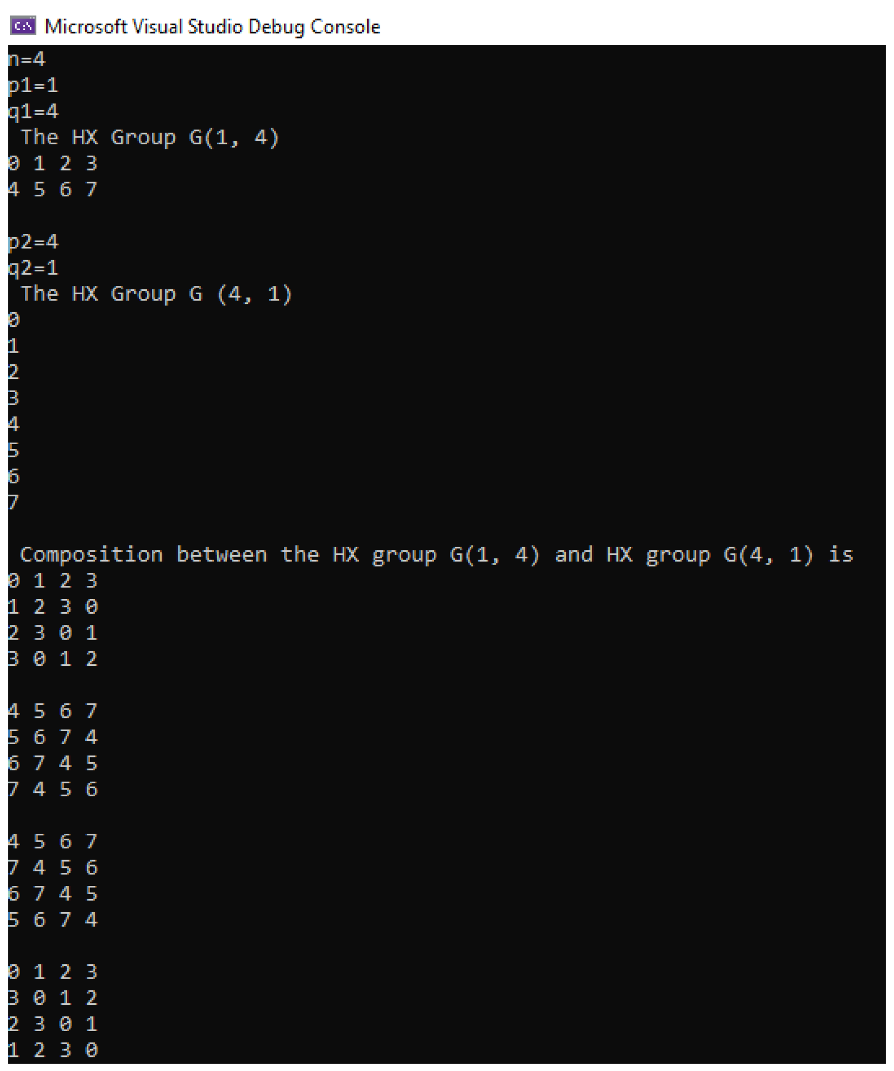
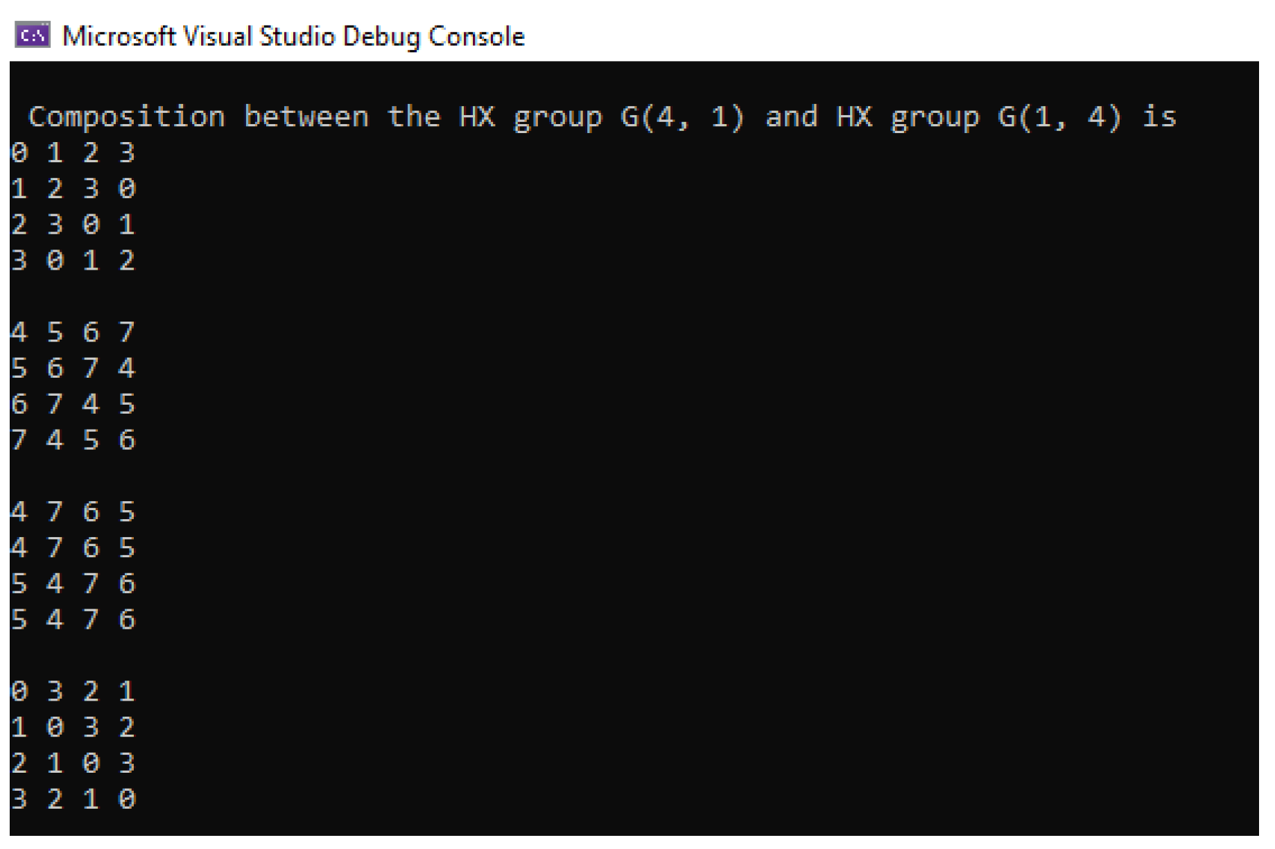
4. Results

4.1. The Results Are Provided by the $\mathit{C}++$ Code Implemented for $N=4$

The following will present the results obtained using the $C++$ code realized in Microsoft Visual Studio 2022. To better understand the above program, we will explain how it works. For $n=4$, we have the hyperstructure

$${\mathcal{G}}_4=\left\{{\mathcal{G}}_2^2,{\mathcal{G}}_1^4,{\mathcal{G}}_4^1\right\}$$

Moreover, we apply the program presented in the previous section in each situation.

First situation: We consider $p_1=2,q_1=2$, $p_2=1,q_2=4,$ respectively. In [16], we presented the composition of HX-groups ${\mathcal{G}}_2^2$ and ${\mathcal{G}}_1^4$. In the presented cod, these HX-groups are equivalent to the following HX-groups

$$\begin{array}{ccc}\hfill {\mathcal{G}}_2^2& =& \left\{\right\{0,2\},\{1,3\},\{4,6\},\{5,7\left\}\right\},\mathrm{where}\hfill \\ \hfill \{0,2\}& =& \left\{f\left({\rho }^0\right),f\left({\rho }^2\right)\right\},\{1,3\}=\left\{f\left({\rho }^1\right),f\left({\rho }^3\right)\right\},\hfill \\ \hfill \{4,6\}& =& \left\{f\left(\sigma \right),f\left({\rho }^2\sigma \right)\right\},\{5,7\}=\left\{f\left(\rho \sigma \right),f\left({\rho }^3\sigma \right)\right\};\hfill \\ \hfill {\mathcal{G}}_1^4& =& \left\{\right\{0,1,2,3\},\{4,5,6,7\left\}\right\},\mathrm{where}\hfill \\ \hfill \{0,1,2,3\}& =& \left\{f\left({\rho }^0\right),f\left({\rho }^1\right),f\left({\rho }^2\right),f\left({\rho }^3\right)\right\},\hfill \\ \hfill \{4,5,6,7\}& =& \left\{f\left(\sigma \right),f\left(\rho \sigma \right),f\left({\rho }^2\sigma \right),f\left({\rho }^3\sigma \right)\right\}.\hfill \end{array}$$

$\left(1\right)$ We compute the elements from case 1, where

$$k\oplus p=f\left({\rho }^k\right)·f\left({\rho }^p\right)=(k+p)\left(modn\right)$$

$$\begin{array}{ccc}\hfill \{0,2\}\oplus \{0,1,2,3\}& =& \left(\bigcup _{k\in \{0,2\}}f\left({\rho }^k\right)\right)\circ \left(\underset{p=0}{\bigcup ^3}f\left({\rho }^p\right)\right)=\hfill \\ & =& 0\oplus 0\cup 0\oplus 1\cup 0\oplus 2\cup 0\oplus 3\cup 2\oplus 0\cup 2\oplus 1\cup 2\oplus 2\cup 2\oplus 3\hfill \\ & =& \{0,1,2,3,2,3,0,1\}=\{0,1,2,3\},\hfill \\ \hfill \{1,3\}\oplus \{0,1,2,3\}& =& \left(\bigcup _{k\in \{1,3\}}f\left({\rho }^k\right)\right)\circ \left(\underset{p=0}{\bigcup ^3}f\left({\rho }^p\right)\right)=\hfill \\ & =& 1\oplus 0\cup 1\oplus 1\cup 1\oplus 2\cup 1\oplus 3\cup 3\oplus 0\cup 3\oplus 1\cup 3\oplus 2\cup 3\oplus 3\hfill \\ & =& \{1,2,3,0,3,0,1,2\}=\{0,1,2,3\}.\hfill \end{array}$$

$\left(2\right)$ We applied the formulas from case $\left(2\right)$, where

$$k\oplus (n+p)=f\left({\rho }^k\right)\circ f\left({\rho }^p\sigma \right)=\left\{\begin{array}{c}n+k+p,k+p<n\\ k+p,k+p\ge n\end{array}\right..$$

$$\begin{array}{ccc}\hfill \{0,2\}\oplus \{4,5,6,7\}& =& \left(\bigcup _{k\in \{0,2\}}f\left({\rho }^k\right)\right)\circ \left(\underset{p=0}{\bigcup ^3}f\left({\rho }^p\sigma \right)\right)=\hfill \\ & =& 0\oplus 4\cup 0\oplus 5\cup 0\oplus 6\cup 0\oplus 7\cup 2\oplus 4\cup 2\oplus 5\cup 2\oplus 6\cup 2\oplus 7\hfill \\ & =& \{4,5,6,7,6,6,4,5\}=\{4,5,6,7\}.\hfill \end{array}$$

We explain the second rule in this situation:

$$\begin{array}{ccc}\hfill 0\oplus 4& =& 4+0+0=4:(k=0,p=0,k+p<4),\hfill \\ \hfill 0\oplus 5& =& 4+0+1=5:(k=0,p=1,k+p<4),\hfill \\ \hfill 0\oplus 6& =& 4+0+2=6:\left(k=0,p=2,k+p<4\right),\hfill \\ \hfill 0\oplus 7& =& 4+0+3=7:\left(k=0,p=3,k+p<4\right),\hfill \\ \hfill 2\oplus 4& =& 4+2+0=6:\left(k=2,p=0,k+p<4\right),\hfill \\ \hfill 2\oplus 5& =& 4+2+1=6:\left(k=2,p=1,k+p<4\right),\hfill \\ \hfill 2\oplus 6& =& 2+2=4:\left(k=2,p=2,k+p\ge 4\right),\hfill \\ \hfill 2\oplus 7& =& 2+3=5:\left(k=2,p=3,k+p\ge 4\right).\hfill \end{array}$$

Similarly, we calculate

$$\begin{array}{ccc}\hfill \{1,3\}\oplus \{4,5,6,7\}& =& \left(\bigcup _{k\in \{1,3\}}f\left({\rho }^k\right)\right)\circ \left(\underset{p=0}{\bigcup ^3}f\left({\rho }^p\sigma \right)\right)=\hfill \\ & =& 1\oplus 4\cup 1\oplus 5\cup 1\oplus 6\cup 1\oplus 7\cup 3\oplus 4\cup 3\oplus 5\cup 3\oplus 6\cup 3\oplus 7\hfill \\ & =& \{5,6,7,4,7,4,5,6\}=\{4,5,6,7\}.\hfill \end{array}$$

$\left(3\right)$ We applied the formulas from case $\left(3\right)$, where

$$(n+p)\oplus k=f\left({\rho }^p\sigma \right)\circ f\left({\rho }^k\right)=\left\{\begin{array}{c}2n+p-k,p<k\\ n+p-k,p\ge k\end{array}\right..$$

$$\begin{array}{ccc}\hfill \{4,6\}\oplus \{0,1,2,3\}& =& \left(\bigcup _{p\in \{0,2\}}f\left({\rho }^p\sigma \right)\right)\circ \left(\underset{k=0}{\bigcup ^3}f\left({\rho }^k\right)\right)=\hfill \\ & =& 4\oplus 0\cup 4\oplus 1\cup 4\oplus 2\cup 4\oplus 3\cup 6\oplus 0\cup 6\oplus 1\cup 6\oplus 2\cup 6\oplus 3\hfill \\ & =& \{4,7,6,5,6,5,4,3\}=\{4,5,6,7\},\hfill \end{array}$$

where

$$\begin{array}{ccc}\hfill 4\oplus 0& =& 4+0-0=4:\left(p=0,k=0,p\ge k\right),\hfill \\ \hfill 4\oplus 1& =& 2\ast 4+0-1=7:\left(p=0,k=1,p<k\right),\hfill \\ \hfill 4\oplus 2& =& 2\ast 4+0-2=6:\left(p=0,k=2,p<k\right),\hfill \\ \hfill 4\oplus 3& =& 2\ast 4+0-3=5:\left(p=0,k=3,p<k\right),\hfill \\ \hfill 6\oplus 0& =& 4+2-0=6:\left(p=2,k=0,p\ge k\right),\hfill \\ \hfill 6\oplus 1& =& 4+2-1=5:\left(p=2,k=1,p\ge k\right),\hfill \\ \hfill 6\oplus 2& =& 4+2-2=4:\left(p=2,k=2,p\ge k\right),\hfill \\ \hfill 6\oplus 3& =& 2\ast 4+2-3=7:\left(p=2,k=3,p<k\right).\hfill \end{array}$$

Analogously, we have

$$\begin{array}{ccc}\hfill \{5,7\}\oplus \{0,1,2,3\}& =& \left(\bigcup _{p\in \{1,3\}}f\left({\rho }^p\sigma \right)\right)\circ \left(\underset{k=0}{\bigcup ^3}f\left({\rho }^k\right)\right)=\hfill \\ & =& 5\oplus 0\cup 5\oplus 1\cup 5\oplus 2\cup 5\oplus 3\cup 7\oplus 0\cup 7\oplus 1\cup 7\oplus 2\cup 7\oplus 3\hfill \\ & =& \{5,4,7,6,7,6,5,4\}=\{4,5,6,7\}.\hfill \end{array}$$

$\left(4\right)$ The fourth case refers to computing the elements that are greater than n. We have the relation

$$(n+p)\oplus (n+k)=f\left({\rho }^p\sigma \right)\circ f\left({\rho }^k\sigma \right)=\left\{\begin{array}{cc}p-k,& p\ge k\\ p+n-k,& p<k\end{array}\right..$$

$$\begin{array}{ccc}\hfill \{4,6\}\oplus \{4,5,6,7\}& =& \left(\bigcup _{p\in \{0,2\}}f\left({\rho }^p\sigma \right)\right)\circ \left(\underset{k=0}{\bigcup ^3}f\left({\rho }^k\sigma \right)\right)=\hfill \\ & =& 4\oplus 4\cup 4\oplus 5\cup 4\oplus 6\cup 4\oplus 7\cup 6\oplus 4\cup 6\oplus 5\cup 6\oplus 6\cup 6\oplus 7\hfill \\ & =& \{0,3,2,1,2,1,0,3\}=\{0,1,2,3\}\hfill \end{array}$$

because

$$\begin{array}{ccc}\hfill 4\oplus 4& =& 0-0=0:\left(p=0,k=0,p\ge k\right);\hfill \\ \hfill 4\oplus 5& =& 0+4-1=3:\left(p=0,k=1,p<k\right);\hfill \\ \hfill 4\oplus 6& =& 0+4-2=2:\left(p=0,k=2,p<k\right);\hfill \\ \hfill 4\oplus 7& =& 0+4-3=1:\left(p=0,k=3,p<k\right);\hfill \\ \hfill 6\oplus 4& =& 2-0=2:\left(p=2,k=0,p\ge k\right);\hfill \\ \hfill 6\oplus 5& =& 2-1=1:\left(p=2,k=1,p\ge k\right);\hfill \\ \hfill 6\oplus 6& =& 2-2=0:\left(p=2,k=2,p\ge k\right);\hfill \\ \hfill 6\oplus 7& =& 2+4-3=3:\left(p=2,k=3,p<k\right).\hfill \end{array}$$

Therefore, ${\mathcal{G}}_2^2\circ {\mathcal{G}}_1^4=\left\{\{0,1,2,3\},\{4,5,6,7\}\right\}={\mathcal{G}}_1^4.$

The composition ${\mathcal{G}}_1^4\circ {\mathcal{G}}_2^2$ is analyzed analogously and will be described in

Table 1. The composition between $HX$-groups ${\mathcal{G}}_1^4$ and ${\mathcal{G}}_2^2$.

${\mathcal{G}}_1^4\circ {\mathcal{G}}_2^2$	$\{0,2\}$	$\{1,3\}$	$\{4,6\}$	$\{5,7\}$
$\{0,1,2,3\}$	$\{0,1,2,3\}$	$\{0,1,2,3\}$	$\{4,5,6,7\}$	$\{4,5,6,7\}$
$\{4,5,6,7\}$	$\{4,5,6,7\}$	$\{4,5,6,7\}$	$\{0,1,2,3\}$	$\{0,1,2,3\}$

:

We have ${\mathcal{G}}_1^4\circ {\mathcal{G}}_2^2=\left\{\{0,1,2,3\},\{4,5,6,7\}\right\}={\mathcal{G}}_1^4$. In conclusion,

$${\mathcal{G}}_2^2\circ {\mathcal{G}}_1^4={\mathcal{G}}_1^4\circ {\mathcal{G}}_2^2={\mathcal{G}}_1^4.$$

Second situation: We consider $p_1=2,q_1=2$, and $p_2=4,q_2=1$ so that the composition ${\mathcal{G}}_2^2\circ {\mathcal{G}}_4^1$ is illustrated in the following table according to the rules presented above for each case.

We can state that ${\mathcal{G}}_2^2\circ {\mathcal{G}}_4^1=\{\{0,2\},\{1,3\},\{4,6\},\{5,7\}\}={\mathcal{G}}_2^2$, and, proceeding similarly, we obtain ${\mathcal{G}}_4^1\circ {\mathcal{G}}_2^2=\{\{0,2\},\{1,3\},\{4,6\},\{5,7\}\}={\mathcal{G}}_2^2$.

Third situation: We have to compute ${\mathcal{G}}_4^1\circ {\mathcal{G}}_1^4$ and ${\mathcal{G}}_1^4\circ {\mathcal{G}}_4^1$, where

$${\mathcal{G}}_4^1=\left\{\left\{0\right\},\left\{1\right\},\left\{2\right\},\left\{3\right\},\left\{4\right\},\left\{5\right\},\left\{6\right\},\left\{7\right\}\right\}.$$

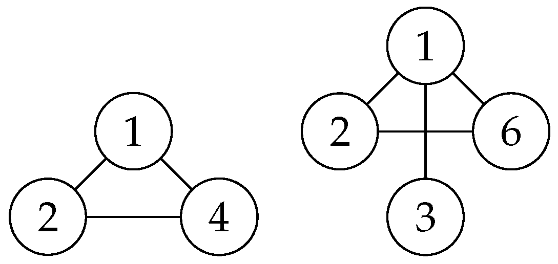
4.2. A Graph Representation of the HX-Groups with Dihedral Group $D_n$ as Support

Graph theory is applied in many fields, such as computer science, physics, biology [4,21,22], and social and information systems. A graph represents connected points along with their connections. Lines or curves can represent these connections. The points are called nodes or vertices; the lines between points are edges. The sets of nodes are denoted by V, and the sets of edges are denoted by E; therefore, a graph is represented by $G=(V,E)$. In this section, we construct the graph associated with the hyperstructures $\left({\mathcal{G}}_4,\circ \right)$ and $\left({\mathcal{G}}_6,\circ \right)$. The vertices represent the elements of the set ${\mathcal{G}}_n$, and we say that $x,y$ formed an edge if and only if

$$[x,y]=x\circ y\cap \{x,y\}\ne \varnothing .$$

(9)

So, let $G_4=(V_4,E_4)$ be the graph associated with the hyperstructures $\left({\mathcal{G}}_4,\circ \right)$, where $V_4=\{{\mathcal{G}}_1^4,{\mathcal{G}}_2^2,{\mathcal{G}}_4^1\}$. In relation (2), we established the connection between the composition of two HX-groups. So, according to them, we can draw the following graphs $G_4$, and, similarly, we obtained the graph $G_6$. For graph $G_4$, the node i is represented by the HX-group ${\mathcal{G}}_i^{{\displaystyle \frac{4}{i}}}$, where i is a divisior of 4, and, for the graph $G_6$, the node j is represented by the HX-group ${\mathcal{G}}_j^{{\displaystyle \frac{6}{j}}}$, where j is a divisior of 6. In graph theory, it is important to determine the degree of a vertex. The degree of a vertex v is denoted by $deg\left(v\right)$ and represents the number of edges that are incident to the vertex. In our situation, we can say that $deg\left(1\right)=deg\left(2\right)=deg\left(4\right)=2$ for $G_4$, and $deg\left(1\right)=3$, $deg\left(2\right)=2$, $deg\left(3\right)=2$, and $deg\left(6\right)=3$ for $G_6$.

5. Discussion

The main objective of the study was to analyze the HX-groups associated with the dihedral group $D_n$ through the IT theory. A code in the $C++$ programming language, created in the Microsoft Visual Studio 2022 program, was presented in detail. This code represents a novelty in the field of HX-groups. In the first part of the paper, we discussed the HX-groups associated with the dihedral group from an algebraic point of view. In the second part of the work, the innovative part of the article was revealed. In Proposition 6, we established a connection between the elements of the dihedral group and natural numbers to implement the HX-groups in the $\mathit{C}++$ code programming language. The compositions between ${\mathcal{G}}_4^1$ and ${\mathcal{G}}_2^2$ and ${\mathcal{G}}_2^2$ and ${\mathcal{G}}_4^1$, respectively, are described in Table 1 and

Table 2. Composition of HX-groups ${\mathcal{G}}_2^2$ and ${\mathcal{G}}_4^1$.

${\mathcal{G}}_2^2\circ {\mathcal{G}}_4^1$	$\left\{0\right\}$	$\left\{1\right\}$	$\left\{2\right\}$	$\left\{3\right\}$	$\left\{4\right\}$	$\left\{5\right\}$	$\left\{6\right\}$	$\left\{7\right\}$
$\{0,2\}$	$\{0,2\}$	$\{1,3\}$	$\{0,2\}$	$\{1,3\}$	$\{4,6\}$	$\{5,7\}$	$\{4,6\}$	$\{5,7\}$
$\{1,3\}$	$\{1,3\}$	$\{0,2\}$	$\{1,3\}$	$\{0,2\}$	$\{5,7\}$	$\{4,6\}$	$\{5,7\}$	$\{4,6\}$
$\{4,6\}$	$\{4,6\}$	$\{5,7\}$	$\{4,6\}$	$\{5,7\}$	$\{0,2\}$	$\{1,3\}$	$\{0,2\}$	$\{1,3\}$
$\{5,7\}$	$\{5,7\}$	$\{4,6\}$	$\{5,7\}$	$\{4,6\}$	$\{1,3\}$	$\{0,2\}$	$\{5,7\}$	$\{0,2\}$

. This code is necessary to improve the calculation time for the composition of two HX-groups. In Figure 1 and Figure 2, we can notice how the program works for $n=4$. Finally, a connection between the HX-groups ${\mathcal{G}}_4$, ${\mathcal{G}}_6$ and graph theory was presented in Figure 3.

References

- Marty, F. Sur une generalization de la notion de group. In Proceedings of the Congress of Scandinavian Mathematicians, Stockholm, Sweden, 14–18 August 1934; pp. 45–49. [Google Scholar]
- Corsini, P.; Leoreanu, V. Applications of Hyperstructures Theory; Kluwer Academic Publishers: Boston, MA, USA; Dordrecht, The Netherlands; London, UK, 2003. [Google Scholar]
- Davvaz, B.; Cristea, I. Fuzzy Algebraic Hyperstructures—An Introduction; Studies in Fuzziness and Soft Computing; Springer: Cham, Switzerland, 2015; Volume 321. [Google Scholar]
- Kalampakas, A.; Spartalis, S.; Tsigkas, A. The Path Hyperoperation. An. Şt. Univ. Ovidius Constanţa 2014, 22, 141–153. [Google Scholar] [CrossRef]
- Linzi, A.; Cristea, I. Dependence Relations and Grade Fuzzy Set. Symmetry 2023, 15, 311. [Google Scholar] [CrossRef]
- Massourous, C.; Mittas, J. Languages-automata and hypercompositional structure. In Algebraic Hyperstructures and Applications, Proceeding of the 4th International Congress, Xanthi, Greece, 27–30 June 1990; World Scientific: Singapore, 1991; pp. 137–147. [Google Scholar]
- Vougiouklis, T. On some representations of hypergroups. Ann. Sci. L’Univ. Clermont Mathématiques 1990, 95, 21–29. [Google Scholar]
- Tofan, I.; Volf, A.C. On some conections between; hyperstructures and fuzzy sets. Ital. J. Pure Appl. Math. 2000, 7, 63–68. [Google Scholar]
- Li, H.X.; Duan, Q.Z.; Wang, P.Z.; Wang, P.Z. Hypergroup(I). BUSEFAL 1985, 23, 22–29. [Google Scholar]
- Li, H.X. HX-groups. BUSEFAL 1987, 33, 31–37. [Google Scholar]
- Zhenliang, Z. The properties of HX-groups. Italian J. Pure Appl. Math. 1997, 2, 97–106. [Google Scholar]
- Corsini, P. HX-groups and Hypergroups. An. Şt. Univ. Ovidius Constanţa 2016, 24, 101–121. [Google Scholar] [CrossRef]
- Corsini, P. HX-Hypergroups associated with the direct product of some Z/nZ. J. Algebr. Struct. Their Appl. 2016, 3, 1–15. [Google Scholar]
- Corsini, P. Hypergroups associated with HX-groups. An. Şt. Univ. Ovidius Constanţa 2017, 25, 49–64. [Google Scholar] [CrossRef]
- Cristea, I.; Novák, M.; Onasanya, B.O. Links Between HX-Groups and Hypergroups. Algebra Coll. 2021, 28, 441–452. [Google Scholar] [CrossRef]
- Sonea, A. HX-groups associated to the dihedral group Dn. J. Mult. Valued Log. Soft Comput. 2019, 33, 11–26. [Google Scholar]
- Sonea, A. A Way to Construct Commutative Hyperstructures. Comput. Sci. Math. Forum. 2023, 7, 22. [Google Scholar] [CrossRef]
- Sonea, A.; Al-Kaseasbeh, S. An introduction to NeutroHX-Groups. In Theory and Applications of NeutroAlgebras as Generalizations of Classical Algebras; IGI Global Publishing Tomorrow’s Research Today: Hershey, PA, USA, 2022. [Google Scholar] [CrossRef]
- Mousavi, S.S.; Jafarpour, M.; Cristea, I. From HX-Groups to HX-Polygroups. Axioms 2024, 13, 7. [Google Scholar] [CrossRef]
- Rotman, J.J. An Introduction to the Theory of Groups; Springer: New York, NY, USA, 1995. [Google Scholar]
- Cristea, I.; Kocijan, J.; Novák, M. Introduction to Dependence Relations and Their Links to Algebraic Hyperstructures. Mathematics 2019, 7, 885. [Google Scholar] [CrossRef]
- Kalampakas, A.; Spartalis, S. Hyperoperations on directed graphs. J. Discret. Math. Sci. Cryptogr. 2023, 27, 1011–1025. [Google Scholar] [CrossRef]
Disclaimer/Publisher’s Note: The statements, opinions and data contained in all publications are solely those of the individual author(s) and contributor(s) and not of MDPI and/or the editor(s). MDPI and/or the editor(s) disclaim responsibility for any injury to people or property resulting from any ideas, methods, instructions or products referred to in the content. |
© 2024 by the authors. Licensee MDPI, Basel, Switzerland. This article is an open access article distributed under the terms and conditions of the Creative Commons Attribution (CC BY) license (https://creativecommons.org/licenses/by/4.0/).
Share and Cite
Sonea, A.P.; Chiruţă, C. Optimizing HX-Group Compositions Using C++: A Computational Approach to Dihedral Group Hyperstructures. Mathematics 2024, 12, 3492. https://doi.org/10.3390/math12223492
Sonea AP, Chiruţă C. Optimizing HX-Group Compositions Using C++: A Computational Approach to Dihedral Group Hyperstructures. Mathematics. 2024; 12(22):3492. https://doi.org/10.3390/math12223492
Chicago/Turabian StyleSonea, Andromeda Pătraşcu, and Ciprian Chiruţă. 2024. "Optimizing HX-Group Compositions Using C++: A Computational Approach to Dihedral Group Hyperstructures" Mathematics 12, no. 22: 3492. https://doi.org/10.3390/math12223492
APA StyleSonea, A. P., & Chiruţă, C. (2024). Optimizing HX-Group Compositions Using C++: A Computational Approach to Dihedral Group Hyperstructures. Mathematics, 12(22), 3492. https://doi.org/10.3390/math12223492