
A Long-Memory Model for Multiple Cycles with an Application to the US Stock Market


Abstract
1. Introduction
2. The Econometric Model
3. The Test Statistic
4. Finite Sample Properties
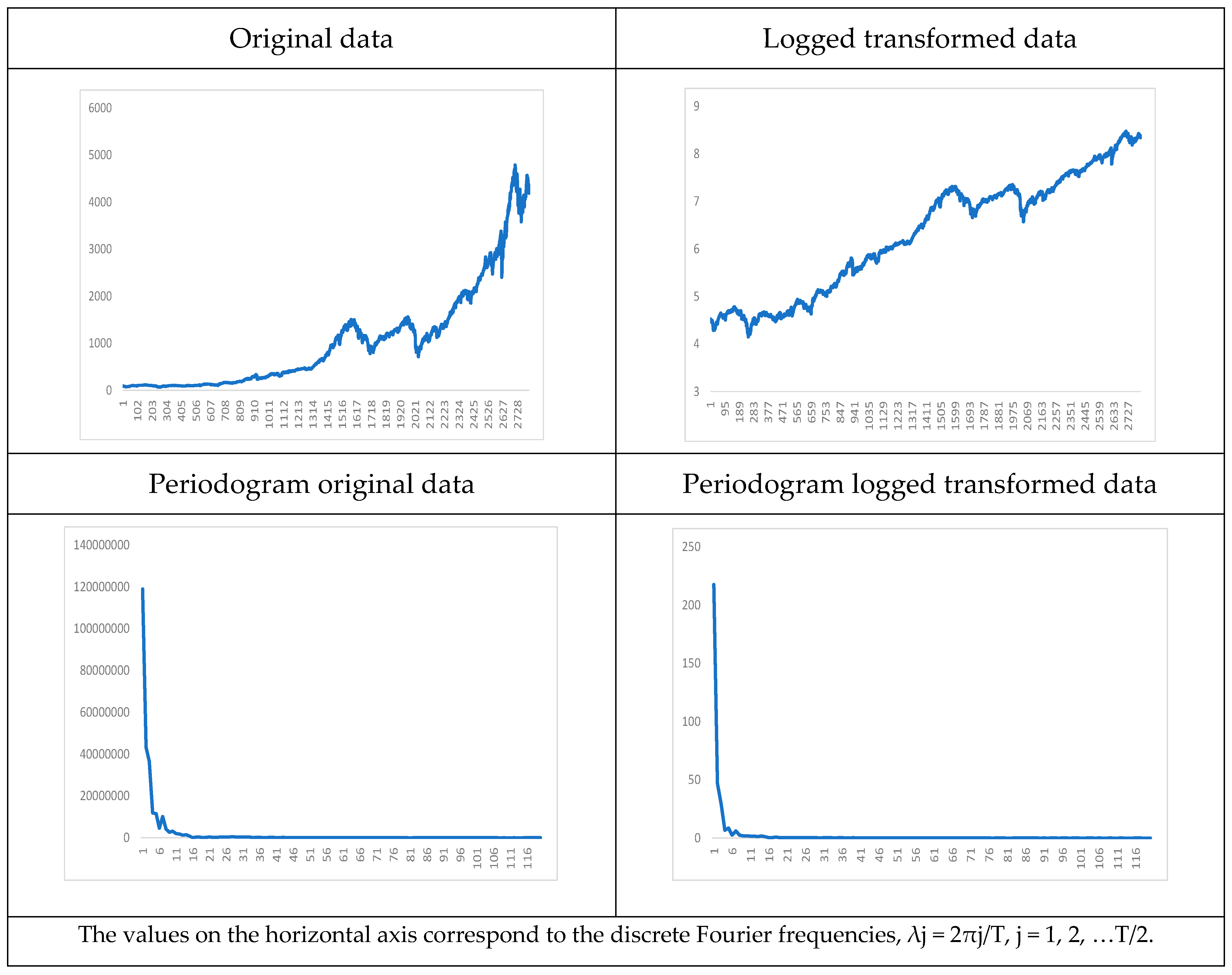
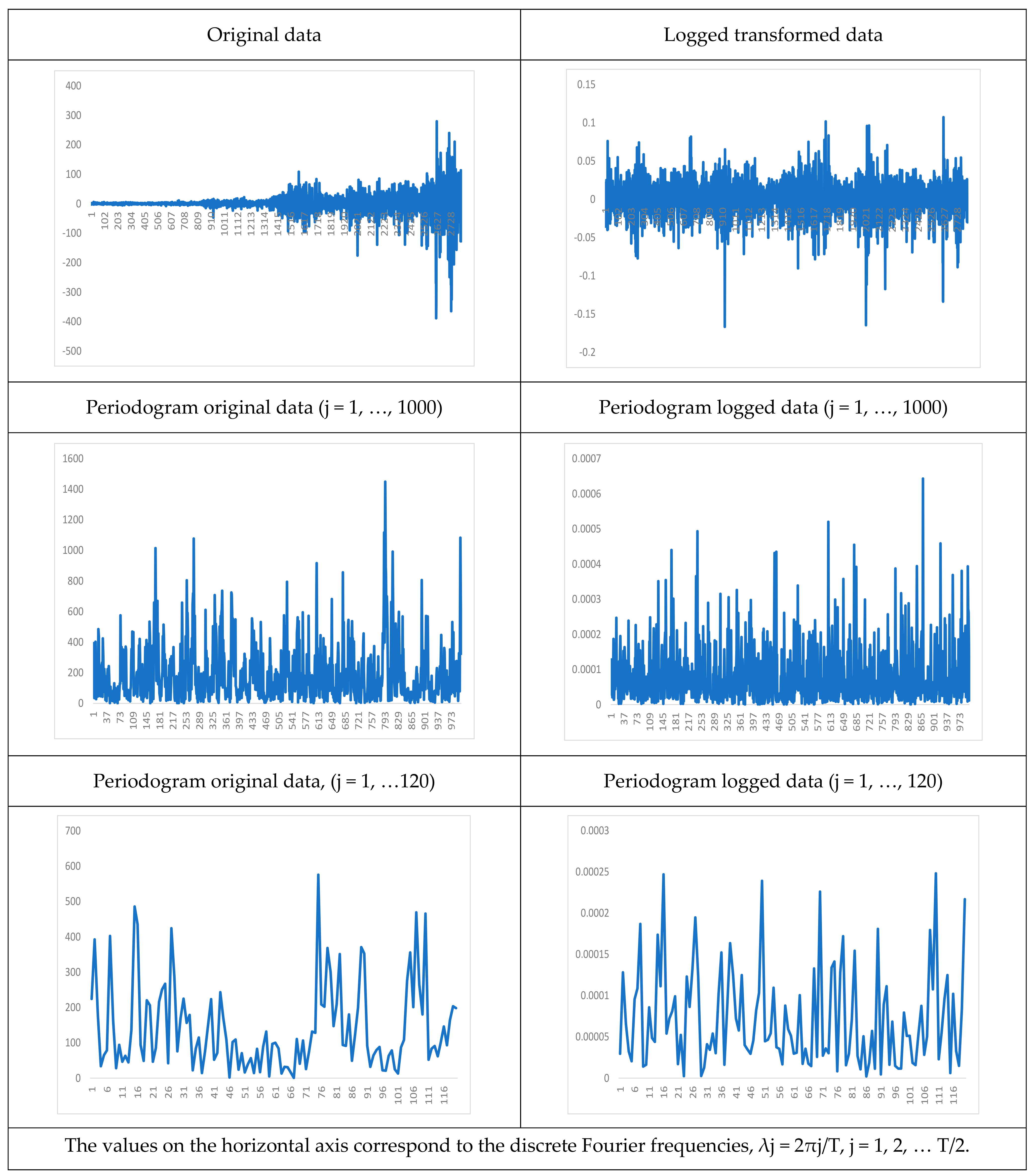
5. An Empirical Application
6. Conclusions
Author Contributions
Funding
Data Availability Statement
Acknowledgments
Conflicts of Interest
References
- Nelson, C.R. Trend/Cycle Decomposition. In The New Palgrave Dictionary of Economics; Palgrave Macmillan: London, UK, 2008. [Google Scholar] [CrossRef]
- Persons, W.M. Indices of business conditions. Rev. Econ. Stat. 1919, 1, 5–107. [Google Scholar]
- Almeida, A.; Brás, S.; Sargento, S.; Pinto, F.C. Time series big data: A survey on data stream frameworks, analysis and algorithms. J. Big Data 2023, 10, 83. [Google Scholar] [CrossRef] [PubMed]
- Robinson, P.M. Efficient tests of nonstationary hypotheses. J. Am. Stat. Assoc. 1994, 89, 1420–1437. [Google Scholar] [CrossRef]
- Bhargava, A. On the theory of testing for unit roots in observed time series. Rev. Econ. Stud. 1986, 52, 369–384. [Google Scholar] [CrossRef]
- Schmdit, P.; Phillips, P.C.B. LM Tests for a Unit Root in the Presence of Deterministic Trends. Oxf. Bull. Econ. Stat. 1992, 54, 257–287. [Google Scholar] [CrossRef]
- Conde-Ruiz, J.I.; García, M.; Puch, L.A.; Ruiz, J. Calendar effects in daily aggregate employment creation and destruction in Spain. SERIEs 2019, 10, 25–63. [Google Scholar] [CrossRef]
- Yaya, O.; Oghonna, A.; Furuoka, F.; Gil-Alana, L.A. A new unit root analysis for testinghysteresis in unemployment. Oxf. Bull. Econ. Stat. 2021, 83, 960–981. [Google Scholar] [CrossRef]
- Gil-Alana, L.A.; Yaya, O. Testing fractional unit roots with non-linear smooth break approximations using Fourier functions. J. Appl. Stat. 2021, 48, 2542–2559. [Google Scholar] [CrossRef]
- Cuestas, J.C.; Gil-Alana, L.A. A non-linear approach with long range dependence based on Chebyshev polynomials. Stud. Nonlinear Dyanmics Econom. 2016, 20, 57–70. [Google Scholar]
- Koumané, E.F.; Hili, O. A new time domain estimation of k-factors GARMA processes. Comptes Rendus Math. 2012, 350, 925–928. [Google Scholar]
- Dickey, D.A.; Fuller, W.A. Distributions of the estimators for autoregressive time series with a unit root. J. Am. Stat. Assoc. 1979, 74, 427–481. [Google Scholar]
- Elliot, G.; Rothenberg, T.J.; Stock, J.H. Efficient tests for an autoregressive unit root. Econometrica 1996, 64, 813–836. [Google Scholar] [CrossRef]
- Geweke, J.; Porter-Hudak, S. The estimation and application of long memory time series models. J. Time Ser. Anal. 1983, 4, 221–223. [Google Scholar] [CrossRef]
- Sowell, F. Maximum Likelihood Estimation of Stationary Univariate Fractionally Integrated Time Series Models. J. Econom. 1992, 53, 165–188. [Google Scholar] [CrossRef]
- Hamming, R.W. Numerical Methods for Scientists and Engineers; Dove Medical Press: Macclesfield, UK, 1973. [Google Scholar]
- Smyth, G.K. Polynomial Approximation; John Wiley & Sons, Ltd.: Hoboken, NJ, USA, 1998. [Google Scholar]
- Bierens, H.J.; Martins, L.F. Time Varying Cointegration. Econom. Theory 2010, 26, 1453–1490. [Google Scholar] [CrossRef]
- Bierens, H.J. Testing the Unit Root with Drift Hypothesis Against Trend Stationarity with an Application to the US Price Level and Interest Rate. J. Econom. 1997, 81, 29–64. [Google Scholar] [CrossRef]
- Tomasevic, N.; Tomasevic, M.; Stanivuk, T. Regression Analysis and Approximation by Means of Chebishev Polynomials. Informatologia 2009, 42, 166–172. [Google Scholar]
- Bloomfield, P. An exponential model in the spectrum of a scalar time series. Biometrika 1973, 60, 217–226. [Google Scholar] [CrossRef]
- Gil-Alana, L.A. The use of the Bloomfield model as an approximation to ARMA processes in the context of fractional integration. Math. Comput. Model. 2004, 39, 429–436. [Google Scholar] [CrossRef]
- Granger, C.W.J. Long memory relationships and the aggregation of dynamic models. J. Econom. 1980, 14, 227–238. [Google Scholar] [CrossRef]
- Granger, C.W.J.; Joyeux, R. An introduction to long memory time series models and fractional differencing. J. Time Ser. Anal. 1980, 1, 15–39. [Google Scholar] [CrossRef]
- Hosking, J.R. Fractional differencing. Biometrika 1981, 68, 165–176. [Google Scholar] [CrossRef]
- Gil-Alana, L.A. Testing Stochastic Cycles in Macroeconomic Time Series. J. Time Ser. Anal. 2001, 22, 411–430. [Google Scholar] [CrossRef]
- Kwiatkowski, D.; Phillips, P.C.; Schmidt, P.; Shin, Y. Testing the null hypothesis of stationarity against the alternative of a unit root. J. Econom. 1992, 54, 159–178. [Google Scholar] [CrossRef]
- Ng, S.; Perron, P. Lag length selection and the Construction of Unit Root Tests with Good Size and Power. Econometrica 2001, 69, 1519–1554. [Google Scholar] [CrossRef]
- Phillips, P.C.B.; Perron, P. Testing for a Unit Root in Time Series Regression. Biometrica 1988, 75, 335–346. [Google Scholar] [CrossRef]
- Ferrara, L.; Guegan, D. Forecasting with k-factor Gegenbauer processes: Theory and Applications. J. Forecast. 2001, 20, 581–601. [Google Scholar] [CrossRef]
- Giraitis, L.; Leipus, P. A generalized fractionally differencing approach in long memory modelling. Lith. Math. J. 1995, 35, 65–81. [Google Scholar] [CrossRef]
- Sadek, N.; Khotanzad, A. K-factor Gegenbauer ARMA process for network traffic simulation. Comput. Commun. 2004, 2, 963–968. [Google Scholar]
- Woodward, W.A.; Cheng, Q.C.; Ray, H.L. A k-factor Gamma long memory model. J. Time Ser. Anal. 1998, 19, 485–504. [Google Scholar] [CrossRef]

| d1 | d2 | d3 | Rejection Freq. |
|---|---|---|---|
| 0.25 | 0.25 | 0.25 | 0.889 |
| 0.25 | 0.25 | 0.50 | 0.947 |
| 0.25 | 0.25 | 0.75 | 1.000 |
| 0.25 | 0.50 | 0.25 | 0.799 |
| 0.25 | 0.50 | 0.50 | 0.845 |
| 0.25 | 0.50 | 0.75 | 0.945 |
| 0.25 | 0.75 | 0.25 | 0.904 |
| 0.25 | 0.75 | 0.50 | 0.967 |
| 0.25 | 0.75 | 0.75 | 1.000 |
| 0.50 | 0.25 | 0.25 | 0.866 |
| 0.50 | 0.25 | 0.50 | 0.923 |
| 0.50 | 0.25 | 0.75 | 0.988 |
| 0.50 | 0.50 | 0.25 | 0.777 |
| 0.50 | 0.50 | 0.50 | 0.814 |
| 0.50 | 0.50 | 0.75 | 0.908 |
| 0.50 | 0.75 | 0.25 | 0.890 |
| 0.50 | 0.75 | 0.50 | 0.923 |
| 0.50 | 0.75 | 0.75 | 0.998 |
| 0.75 | 0.25 | 0.25 | 0.815 |
| 0.75 | 0.25 | 0.50 | 0.901 |
| 0.75 | 0.25 | 0.75 | 0.945 |
| 0.75 | 0.50 | 0.25 | 0.119 |
| 0.75 | 0.50 | 0.50 | 0.807 |
| 0.75 | 0.50 | 0.75 | 0.833 |
| 0.75 | 0.75 | 0.25 | 0.812 |
| 0.75 | 0.75 | 0.50 | 0.865 |
| 0.75 | 0.75 | 0.75 | 0.939 |
| d1 | d2 | d3 | Rejection Freq. |
|---|---|---|---|
| 0.25 | 0.25 | 0.25 | 0.911 |
| 0.25 | 0.25 | 0.50 | 1.000 |
| 0.25 | 0.25 | 0.75 | 1.000 |
| 0.25 | 0.50 | 0.25 | 0.801 |
| 0.25 | 0.50 | 0.50 | 0.906 |
| 0.25 | 0.50 | 0.75 | 1.000 |
| 0.25 | 0.75 | 0.25 | 0.998 |
| 0.25 | 0.75 | 0.50 | 1.000 |
| 0.25 | 0.75 | 0.75 | 1.000 |
| 0.50 | 0.25 | 0.25 | 0.899 |
| 0.50 | 0.25 | 0.50 | 0.978 |
| 0.50 | 0.25 | 0.75 | 1.000 |
| 0.50 | 0.50 | 0.25 | 0.839 |
| 0.50 | 0.50 | 0.50 | 0.848 |
| 0.50 | 0.50 | 0.75 | 0.922 |
| 0.50 | 0.75 | 0.25 | 0.955 |
| 0.50 | 0.75 | 0.50 | 0.988 |
| 0.50 | 0.75 | 0.75 | 1.000 |
| 0.75 | 0.25 | 0.25 | 0.890 |
| 0.75 | 0.25 | 0.50 | 0.977 |
| 0.75 | 0.25 | 0.75 | 0.994 |
| 0.75 | 0.50 | 0.25 | 0.094 |
| 0.75 | 0.50 | 0.50 | 0.883 |
| 0.75 | 0.50 | 0.75 | 0.847 |
| 0.75 | 0.75 | 0.25 | 0.890 |
| 0.75 | 0.75 | 0.50 | 0.914 |
| 0.75 | 0.75 | 0.75 | 0.978 |
| d1 | d2 | d3 | Rejection Freq. |
|---|---|---|---|
| 0.25 | 0.25 | 0.25 | 0.989 |
| 0.25 | 0.25 | 0.50 | 1.000 |
| 0.25 | 0.25 | 0.75 | 1.000 |
| 0.25 | 0.50 | 0.25 | 0.991 |
| 0.25 | 0.50 | 0.50 | 0.911 |
| 0.25 | 0.50 | 0.75 | 1.000 |
| 0.25 | 0.75 | 0.25 | 1.000 |
| 0.25 | 0.75 | 0.50 | 1.000 |
| 0.25 | 0.75 | 0.75 | 1.000 |
| 0.50 | 0.25 | 0.25 | 0.939 |
| 0.50 | 0.25 | 0.50 | 1.000 |
| 0.50 | 0.25 | 0.75 | 1.000 |
| 0.50 | 0.50 | 0.25 | 0.965 |
| 0.50 | 0.50 | 0.50 | 0.934 |
| 0.50 | 0.50 | 0.75 | 0.980 |
| 0.50 | 0.75 | 0.25 | 0.999 |
| 0.50 | 0.75 | 0.50 | 1.000 |
| 0.50 | 0.75 | 0.75 | 1.000 |
| 0.75 | 0.25 | 0.25 | 0.956 |
| 0.75 | 0.25 | 0.50 | 1.000 |
| 0.75 | 0.25 | 0.75 | 0.999 |
| 0.75 | 0.50 | 0.25 | 0.066 |
| 0.75 | 0.50 | 0.50 | 0.909 |
| 0.75 | 0.50 | 0.75 | 0.917 |
| 0.75 | 0.75 | 0.25 | 0.943 |
| 0.75 | 0.75 | 0.50 | 0.993 |
| 0.75 | 0.75 | 0.75 | 1.000 |
| (i) Results Based on White Noise Errors | |||
| No Terms | With an Intercept | With a Time Trend | |
| Original | 0.97 (0.94, 1.00) | 0.97 (0.94, 1.00) | 0.97 (0.94, 1.00) |
| Logged values | 0.99 (0.96, 1.02) | 0.98 (0.96, 1.01) | 0.98 (0.96, 1.01) |
| (ii) Results Based on Autocorrelated (Bloomfield) Errors | |||
| No Terms | With an Intercept | With a Time Trend | |
| Original | 0.95 (0.92, 0.99) | 0.95 (0.92, 1.00) | 0.95 (0.92, 1.00) |
| Logged values | 0.97 (0.93, 1.02) | 0.99 (0.95, 1.04) | 0.99 (0.95, 1.04) |
| (i) Results Based on White Noise Errors | |||||
| D | θ1 | θ2 | θ3 | θ4 | |
| Original | 0.97 (0.93, 1.01) | 1811.38 (1.92) | −1381.76 (−2.44) | 484.63 (1.67) | −335.25 (−1.72) |
| Logged | 1.01 (0.98, 1.04) | 5.400 (6.81) | −0.058 (−0.12) | −0.575 (−2.39) | 1.167 (7.30) |
| (ii) Results Based on Autocorrelated (Bloomfield) Errors | |||||
| D | θ1 | θ2 | θ3 | θ4 | |
| Original | 0.96 (0.94, 1.02) | 1043.07 (1.59) | −702.52 (−1.93) | 307.28 (1.48) | −185.24 (−1.32) |
| Logged | 1.00 (0.97, 1.04) | 0.915 (6.81) | −3.429 (−4.32) | 1.096 (2.77) | 0.047 (0.17) |
| (1 − L) Data | (1 − L) Log Data | ||||
|---|---|---|---|---|---|
| j | T/j | Value at Periodogram | J | T/j | Value at Periodogram |
| 794 | 3.53 | 1448.09 | 871 | 3.22 | 0.000642 |
| 998 | 2.81 | 1082.75 | 607 | 4.62 | 0.000520 |
| 274 | 10.24 | 1076.58 | 242 | 11.60 | 0.000493 |
| 170 | 16.51 | 1013.94 | 920 | 3.05 | 0.000458 |
| 814 | 3.45 | 990.76 | 679 | 4.13 | 0.000454 |
| 608 | 4.61 | 916.17 | 170 | 16.51 | 0.000639 |
| (1 − L) Data | (1 − L) Log Data | ||||
|---|---|---|---|---|---|
| j | T/j | Value at Periodogram | J | T/j | Value at Periodogram |
| 75 | 37.44 | 575.65 | 110 | 25.52 | 0.000248 |
| 15 | 187.20 | 485.48 | 16 | 175.50 | 0.000247 |
| 107 | 26.25 | 469.23 | 50 | 56.16 | 0.000239 |
| 110 | 25.52 | 465.70 | 70 | 40.11 | 0.000226 |
| j1 | j2 | j3 | d1 | d2 | d3 | |
|---|---|---|---|---|---|---|
| White noise | 602 (4.66) | 240 (11.70) | 14 (200.57) | 0.09 (0.02, 1.17) | 0.06 (0.01, 0.09) | 0.13 (0.11, 0.14) |
| Bloomfield | 601 (4.67) | 241 (11.65) | 14 (200.57) | 0.06 (−0.01, 1.17) | 0.07 (0.02, 0.10) | 0.05 (−0.02, 0.10) |
| j1 | j2 | j3 | d1 | d2 | d3 | |
|---|---|---|---|---|---|---|
| White noise | 600 (4.69) | 236 (11.89) | 13 (216.00) | 0.07 (−0.01, 0.14) | 0.04 (−0.05, 0.08) | 0.12 (0.05, 0.16) |
| Bloomfield | 609 (4.61) | 238 (11.78) | 14 (200.57) | 0.05 (−0.02, 0.19) | 0.03 (−0.03, 0.07) | 0.11 (0.04, 0.17) |
Disclaimer/Publisher’s Note: The statements, opinions and data contained in all publications are solely those of the individual author(s) and contributor(s) and not of MDPI and/or the editor(s). MDPI and/or the editor(s) disclaim responsibility for any injury to people or property resulting from any ideas, methods, instructions or products referred to in the content. |
© 2024 by the authors. Licensee MDPI, Basel, Switzerland. This article is an open access article distributed under the terms and conditions of the Creative Commons Attribution (CC BY) license (https://creativecommons.org/licenses/by/4.0/).
Share and Cite
Caporale, G.M.; Gil-Alana, L.A. A Long-Memory Model for Multiple Cycles with an Application to the US Stock Market. Mathematics 2024, 12, 3487. https://doi.org/10.3390/math12223487
Caporale GM, Gil-Alana LA. A Long-Memory Model for Multiple Cycles with an Application to the US Stock Market. Mathematics. 2024; 12(22):3487. https://doi.org/10.3390/math12223487
Chicago/Turabian StyleCaporale, Guglielmo Maria, and Luis Alberiko Gil-Alana. 2024. "A Long-Memory Model for Multiple Cycles with an Application to the US Stock Market" Mathematics 12, no. 22: 3487. https://doi.org/10.3390/math12223487
APA StyleCaporale, G. M., & Gil-Alana, L. A. (2024). A Long-Memory Model for Multiple Cycles with an Application to the US Stock Market. Mathematics, 12(22), 3487. https://doi.org/10.3390/math12223487