A New Extragradient-Viscosity Method for a Variational Inequality, an Equilibrium Problem, and a Fixed Point Problem

Abstract

In this research article, we introduce a novel iterative approach that builds upon a two-step extragradient-viscosity method. This method aims to find a common element among the solution set of a variational inequality, an equilibrium problem, and the set of common fixed points from a countable family of demicontractive mappings in a Hilbert space. We offer a robust convergence theorem for the proposed iterative scheme, considering certain well-conditioned parameters. Our findings represent an improvement over similar results already available in the existing literature. Furthermore, we demonstrate the applicability of our main result to W-mappings. Lastly, we present two numerical examples to exhibit the consistency and accuracy of our devised scheme.

1. Introduction

Consider a real Hilbert space H with inner product $⟨·,·⟩$ and norm $\parallel · \parallel$. Let C denote a nonempty closed convex subset of H. A mapping $T:C\to C$ is defined as nonexpansive if it satisfies the inequality $\parallel Tx-Ty\parallel \le \parallel x-y\parallel$ for all $x,y\in C$.

In this paper, we address the equilibrium problem (EP) defined by finding a point $u\in C$ such that:

$$\begin{array}{c}\hfill \varphi (u,v)\ge 0\mathrm{for}\mathrm{all}v\in C,\end{array}$$

(1)

where $\varphi :C\times C\to \mathbb{R}$ is a bifunction. The solution set of this equilibrium problem is denoted by $EP\left(\varphi \right)=\{u\in C$: (1) holds}. Equilibrium problems have broad applications across diverse fields such as physics, optimization, finance, game theory, and economics. They encompass various models including mathematical programming, variational inequalities, complementarity problems, saddle point problems, Nash equilibrium in games, minimization problems, and fixed point problems, as referenced in the literature [1,2,3,4,5,6,7,8,9,10,11,12,13].

Setting $\varphi (x,y)=⟨Ax,y-x⟩$ for $x,y\in C$, where $A:C\to H$ is a nonlinear operator, transforms EP (1) into the classical variational inequality problem (VIP):

$$\begin{array}{c}\hfill \mathrm{Find}{x}^{*}\in C\mathrm{such}\mathrm{that}⟨A{x}^{*},y-x^{*}⟩\ge 0\mathrm{for}\mathrm{all}y\in C,\end{array}$$

(2)

introduced by Hartmann and Stampacchia [14]. The set of solutions to (2) is denoted by $VI(A,C)$. Various methods for solving VIPs have been developed, such as the extragradient method (EGM) proposed by Korpelevich [15] in 1976, which generates two sequences through:

$$\begin{array}{c}\hfill \left\{\begin{array}{c}{y}_n=P_C(x_n-\lambda A{x}_n),\hfill \\ x_{n+1}=P_C(x_n-\lambda A{y}_n),\hfill \end{array}\right.\end{array}$$

(3)

where $\lambda >0$ is a parameter and $A:C\to {\mathbb{R}}^n$ is a monotone and Lipschitzian continuous operator. Subsequent improvements to EGM include the subgradient extragradient algorithm (SEGM) introduced by Censor et al. [16], which modifies the projection process to simplify computation:

$$\begin{array}{c}\hfill \left\{\begin{array}{c}{y}_n=P_C(x_n-\lambda A{x}_n),\hfill \\ C_n=\{v\in H:⟨x_n-\lambda A{x}_n-y_n,v-y_n⟩\le 0\},\hfill \\ x_{n+1}=P_{C_n}(x_n-\lambda A{y}_n).\hfill \end{array}\right.\end{array}$$

(4)

The SEGM method offers computational advantages by replacing the second projection with a projection onto a half-space, under certain assumptions.

The fixed point problem (FPP), on the other hand, involves finding $x^{*}\in C$ such that:

$$\begin{array}{c}\hfill T{x}^{*}=x^{*},\end{array}$$

(5)

where $T:C\to C$ is a nonlinear mapping. The solution set of (5) is denoted by $Fix\left(T\right)=\{x\in C:Tx=x\}$.

We are also interested in finding a common solution to both VIP (2) and FPP (5), which can be expressed as:

$$\begin{array}{c}\hfill \mathrm{Find}{x}^{*}\in VI(A,C)\cap Fix\left(T\right).\end{array}$$

(6)

Recent studies have explored iterative schemes for solving this combined problem. For example, Nadezhkina and Takahashi [17] proposed an iterative scheme based on EGM, which is formulated as:

$$\begin{array}{c}\hfill \left\{\begin{array}{c}{y}_n=P_C(x_n-{\lambda }_{n}A{x}_n),\hfill \\ x_{n+1}=(1-{\alpha }_n)x_n+{\alpha }_{n}T{P}_C(x_n-{\lambda }_{n}A{y}_n),\hfill \end{array}\right.\end{array}$$

(7)

where T is nonexpansive and A is monotone and L-Lipschitzian continuous. The authors showed that the sequence $\left\{x_n\right\}$ converges weakly to a solution of (6) (see [16,18,19,20]).

For strong convergence, Censor et al. [21] proposed a hybrid scheme combining SEGM and a method that includes:

$$\begin{array}{c}\hfill \left\{\begin{array}{c}{y}_n=P_C(x_n-\lambda A{x}_n),\hfill \\ C_n=\{v\in H:⟨x_n-\lambda A{x}_n-y_n,v-y_n⟩\le 0\},\hfill \\ z_n=P_{C_n}(x_n-\lambda A{y}_n),\hfill \\ t_n={\alpha }_n{x}_n+(1-{\alpha }_n)({\beta }_n{z}_n+(1-{\beta }_n)T{z}_n),\hfill \\ Q_n=\{z\in H:\parallel t_n-z\parallel \le \parallel t_n-z\parallel \},\hfill \\ S_n=\{z\in H:⟨x_n-z,x_n-x_0⟩\le 0\},\hfill \\ x_{n+1}=P_{Q_n\cap S_n}\left(x_0\right).\hfill \end{array}\right.\end{array}$$

(8)

After that, Maingé [18] proposed a hybrid extragradient-viscosity method (HEGVM) to address (6) without requiring projection onto the intersection of sets:

$$\begin{array}{c}\hfill \left\{\begin{array}{c}{y}_n=P_C(x_n-{\lambda }_{n}A{x}_n),\hfill \\ z_n=P_C(x_n-{\lambda }_{n}A{y}_n),\hfill \\ x_{n+1}=(1-\omega )I{x}_n+\omega T{t}_n,t_n=z_n-{\alpha }_{n}F{z}_n,\hfill \end{array}\right.\end{array}$$

(9)

where A is monotone and Lipschitzian, T is demicontractive, F is an operator, and ${\lambda }_n,$${\alpha }_n>0$, $\omega \in [0,1]$ are parameters. This method guarantees strong convergence to the unique solution of the variational inequality.

In this work, we propose a new iterative scheme for finding a common solution to the equilibrium problem (EP), variational inequality (VIP), and fixed point problem (FPP). Our method, based on the two-step extragradient-viscosity approach, aims to solve the composite problem:

$$\begin{array}{c}\hfill ⟨F{x}^{*},p-x^{*}⟩\ge 0\mathrm{for}\mathrm{all}p\in \Gamma ,\end{array}$$

(10)

where $\Gamma =EP\left(\varphi \right)\cap VI(A,C)\cap Fix\left(T\right)$ and $F:H\to H$ is an operator meeting certain conditions. We present a strong convergence theorem for our scheme and demonstrate its effectiveness through numerical examples.

2. Preliminaries

Let H be a real Hilbert space. We denote weak convergence by ⇀ and strong convergence by → in H. The following identity holds:

$$\begin{array}{cc}\hfill {|\alpha x+\beta y+\gamma z|}^2=& {\alpha \left|x\right|}^2+{\beta \left|y\right|}^2+\gamma {\left|z\right|}^2\hfill \\ \hfill & {-\alpha \beta |x-y|}^2{-\beta \gamma |z-y|}^2-\alpha \gamma {|z-x|}^2,\hfill \end{array}$$

for all $x,y,z\in H$ and $\alpha ,\beta ,\gamma \in [0,1]$ such that $\alpha +\beta +\gamma =1$.

Let C be a nonempty, closed, convex subset of H. For any $x\in H$, there exists a unique nearest point in C, denoted by $P_C\left(x\right)$, such that

$$\begin{array}{c}\hfill |x-P_C\left(x\right)|\le |x-y|\mathrm{for}\mathrm{all}y\in C.\end{array}$$

The mapping $P_C$ is referred to as the metric projection of H onto C, and it is known that $P_C$ is nonexpansive.

Lemma 1. 

Let $P_C$ be the metric projection of H onto C. Then,

 (i) 

$\parallel x-P_C{y\parallel }^2+\parallel P_C{y-y\parallel }^2\le {\parallel x-y\parallel }^2\mathit{for}\mathit{all}x\in C,y\in H.$

 (ii) 

$z=P_C\left(x\right)\iff ⟨x-z,z-y⟩\ge 0\mathit{for}\mathit{all}y\in C.$

Definition 1. 

A mapping $T:H\to H$ is called firmly nonexpansive if, for any $x,y\in H,$

$$\begin{array}{c}\hfill {\parallel Tx-Ty\parallel }^2\le ⟨Tx-Ty,x-y⟩.\end{array}$$

Lemma 2 

([1]). Let C be a nonempty closed convex subset of H and $\varphi :C\times C\to \mathbb{R}$ be a bifunction satisfying the following conditions:

($A_1$)

$\varphi (x,x)=0$ for all $x\in C$;

($A_2$)

ϕ is monotone, i.e., $\varphi (x,y)+\varphi (y,x)\le 0$, for all $x,y\in C$;

($A_3$)

For each $x,y,z\in C,$ ${lim}_{t\downarrow 0}\varphi (tz+(1-t)x,y)\le \varphi (x,y)$;

($A_4$)

For each $x\in C,y\mapsto \varphi (x,y)$ is convex and weakly lower semicontinuous.

Let $r>0$ and $x\in H$. Then, there exists $z\in C$ such that

$$\begin{array}{c}\hfill \varphi (z,y)+{\displaystyle \frac{1}{r}}⟨y-z,z-x⟩\ge 0,\mathit{for}\mathit{all}y\in C.\end{array}$$

Lemma 3 

([22]). Assume $\varphi :C\times C\to \mathbb{R}$ satisfies the conditions ($A_1$)–($A_4$). For $r>0$, define a mapping $Q_r:H\to C$ by

$$\begin{array}{c}\hfill Q_{r}x:=\{z\in C:\varphi (z,y)+{\displaystyle \frac{1}{r}}⟨y-z,z-x⟩\ge 0,\forall y\in C\}\end{array}$$

(11)

for all $x\in H$. Then, the following hold:

 (i) 

$Q_r$ is single-valued;

 (ii) 

$Q_r$ is firmly nonexpansive;

 (iii) 

$Fix\left(Q_r\right)=EP\left(\varphi \right)$;

 (iv) 

$EP\left(\varphi \right)$ is closed and convex.

Definition 2. 

Assume $T:H\to H$ is a mapping. Then, $I-T$ is said to be demiclosed at zero if, for any $\left\{x_n\right\}$ in H, the following implication holds:

$$\begin{array}{c}\hfill x_n\rightharpoonup x\mathit{and}(I-T)x_n\to 0\Rightarrow x\in Fix\left(T\right).\end{array}$$

It is well known that each nonexpansive mapping is demiclosed at zero.

Definition 3. 

Let $T:H\to H$ be a mapping with $Fix\left(T\right)\ne \varnothing$. Then,

 (i) 

$T:H\to H$ is called quasi-nonexpansive if

$$\begin{array}{c}\hfill \parallel Tx-z\parallel \le \parallel x-z\parallel ,\forall z\in Fix\left(T\right),x\in H.\end{array}$$

 (ii) 

$T:H\to H$ is called β-demicontractive with $0\le \beta <1$ if

$$\begin{array}{c}\hfill {\parallel Tx-z\parallel }^2\le {\parallel x-z\parallel }^2+\beta {\parallel x-Tx\parallel }^2,\forall z\in Fix\left(T\right),x\in H.\end{array}$$

Definition 4. 

$F:H\to H$ is an operator. Then,

F is called L-Lipschitzian continuous ($L>0$) if

$$\begin{array}{c}\hfill \parallel Fx-Fy\parallel \le L\parallel x-y\parallel \mathit{for}\mathit{all}x,y\in H.\end{array}$$

F is called η-strongly monotone ($\eta >0$) if

$$\begin{array}{c}\hfill ⟨Fx-Fy,x-y⟩\ge {\eta \parallel x-y\parallel }^2\mathit{for}\mathit{all}x,y\in H.\end{array}$$

Lemma 4 

([18]). Assume that $T:C\to C$ is a β-demicontractive mapping with $Fix\left(T\right)\ne \varnothing$. Then,

 (i) 

$S_{\omega }=(1-\omega )I+\omega TwS$ is a quasi-nonexpansive mapping over C for every $\omega \in [0,1-\beta ]$. Furthermore,

$$\begin{array}{c}\hfill \parallel S_{\omega }x-x^{*}{\parallel }^2\le \parallel x-x^{*}{\parallel }^2-\omega (1-\beta -\omega ){\parallel Tx-x\parallel }^2,\forall x^{*}\in Fix\left(T\right),\forall x\in C.\end{array}$$

 (ii) 

Fix(T) is closed and convex.

Recall that the normal cone $N_C$ of C at a point $x\in C$ is defined by

$$\begin{array}{c}\hfill N_C\left(x\right)=\{\omega \in H:⟨\omega ,x-y⟩\ge 0,\forall y\in C\}.\end{array}$$

Lemma 5 

([23]). Let $F:H\to H$ be an η-strongly monotone and L-Lipschitzian continuous mapping and $0<\mu <{\displaystyle \frac{2\eta }{L^2}}$. Define the mapping $G:H\to H$ by

$$\begin{array}{c}\hfill G^{\mu }\left(x\right)=(I-\mu F)x,x\in H.\end{array}$$

Then,

 (i) 

$G^{\mu }$ is a Lipschitzian continuous mapping on H with the constant $\sqrt{1-\mu (2\eta -\mu L^2)}$.

 (ii) 

For all $\nu \in (0,\mu )$, we obtain

$$\begin{array}{c}\hfill \parallel G^{\nu }\left(y\right)-x\parallel \le (1-{\displaystyle \frac{\nu \tau }{\mu }})\parallel y-x\parallel +\nu \parallel Fx\parallel ,\end{array}$$

for all $x,y\in H$, where $\tau =1-\sqrt{1-\mu (2\eta -\mu L^2)}\in (0,1)$.

Definition 5. 

Let C be a nonempty closed bounded subset of H. An operator $A:H\to H$ is called maximal monotone on C if it is monotone on C and its graph $G\left(A\right):=\left\{\right(x,Ax):x\in C\}$ is not a proper subset of the graph of any other monotone mapping.

Lemma 6 

([24]). Let C be a nonempty closed convex subset of H and let A be a monotone and Lipschitzian continuous (even hemi-continuous) mapping of C into H with $D\left(A\right)=C$. Let Q be a mapping defined by

$$\begin{array}{c}\hfill Q\left(x\right)=\left\{\begin{array}{c}Ax+N_{C}x\mathit{if}x\in C\hfill \\ \varnothing \mathit{if}x\notin C.\hfill \end{array}\right.\end{array}$$

Then, Q is maximal monotone and $Q^{-1}0=VI(A,C)$.

Lemma 7 

([25]). Let C be a nonempty closed bounded subset of H. Suppose

$$\sum _{n=1}^{\infty }sup\{\parallel T_{n+1}z-T_{n}z\parallel :z\in C\}<\infty .$$

Then, for each $y\in C$, $\left\{T_{n}y\right\}$ converges strongly to some point of C. Moreover, let T be a mapping of C into itself defined by $Ty={lim}_{n\to \infty }{T}_{n}y$ for all $y\in C$. Then, ${lim}_{n\to \infty }sup\{\parallel Tz-T_{n}z\parallel :z\in C\}=0$.

Lemma 8 

([18]). Let $\left\{a_n\right\}$ be a sequence of non-negative real numbers which is not decreasing at infinity in the sense that there exists a subsequence $\left\{a_{n_j}\right\}$ of $\left\{a_n\right\}$ such that $a_{n_j}<a_{n_j+1}$ for all $j\in \mathbb{N}$. Then, there exists a nondecreasing subsequence $\left\{m_k\right\}$ of $\mathbb{N}$ such that ${lim}_{k\to \infty }{m}_k=\infty$ and the following properties are satisfied for all (sufficiently large) numbers $k\in \mathbb{N}$:

$$\begin{array}{c}\hfill a_{m_k}\le a_{m_k+1}\mathit{and}{a}_k\le a_{m_k+1}.\end{array}$$

In fact, for each k, $m_k$ is the largest number $n\in \{1,2,\dots ,k\}$ such that $a_n<a_{n+1}$.

3. Main Result

Lemma 9. 

Let $A:H\to H$ be monotone on C and a κ-Lipschitzian continuous mapping on H, and let $\varphi :H\times H\to \mathbb{R}$ be a bifunction satisfying the conditions $\left(A_1\right)$–$\left(A_4\right)$ of Lemma 2 and $\Omega :=VI(A,C)\cap EP\left(\varphi \right)\ne \varnothing$. Suppose that three parameters r, μ, and λ satisfy the conditions $r>0$, $0<\lambda <{\displaystyle \frac{1}{3\kappa }}$, and $0\le \mu \le \lambda$. Let $x\in H$ and

$$u=Q_{r}x,y=P_C(u-\mu Au),z=P_C(y-\lambda Ay),v=P_C(u-\lambda Az).$$

Then,

 (i) 

$\parallel v-z\parallel \le \parallel u-y\parallel +\lambda \kappa \parallel y-z\parallel$.

 (ii) 

${\parallel v-p\parallel }^2\le {\parallel x-p\parallel }^2{-\parallel u-x\parallel }^2{-(1-3\lambda \kappa )(\parallel u-y\parallel }^2{+\parallel y-z\parallel }^2)$ for all $p\in \Omega$.

 Proof. 

(i)

Since $P_C$ is nonexpansive and A is a $\kappa$-Lipschitzian mapping, we obtain

$$\begin{array}{cc}\hfill \parallel v-z\parallel & \le \parallel P_C(u-\lambda Az)-P_C(y-\lambda Ay)\parallel \le \parallel (u-\lambda Az)-(y-\lambda Ay)\parallel \hfill \\ \hfill & \le \parallel u-y\parallel +\lambda \kappa \parallel y-z\parallel .\hfill \end{array}$$

(ii)

Let $p\in \Omega$. Noticing $u=Q_{r}x$ and $Q_{r}p=p$, it follows from Lemma 3 (ii) that

$$\begin{array}{cc}\hfill {\parallel u-p\parallel }^2=& \parallel Q_{r}x-Q_r{p\parallel }^2\le ⟨x-p,u-p⟩\hfill \\ \hfill =& {\displaystyle \frac{1}{2}}{(\parallel x-p\parallel }^2{+\parallel u-p\parallel }^2{-\parallel u-x\parallel }^2).\hfill \end{array}$$

This implies

$$\begin{array}{c}\hfill {\parallel u-p\parallel }^2\le {\parallel x-p\parallel }^2-{\parallel u-x\parallel }^2.\end{array}$$

(12)

Moreover, from the definition of v and Lemma 1 (i), we have

$$\begin{array}{cc}\hfill {\parallel v-p\parallel }^2& \le {\parallel u-\lambda Az-p\parallel }^2-{\parallel u-\lambda Az-v\parallel }^2\hfill \\ \hfill & ={\parallel u-p\parallel }^2-{\parallel u-v\parallel }^2-2\lambda ⟨Az,v-p⟩.\hfill \end{array}$$

(13)

From $p\in VI(A,C)$, $⟨Ap,z-p⟩\ge 0$. Since A is monotone, we obtain

$$\begin{array}{c}\hfill ⟨Az,z-p⟩\ge ⟨Ap,z-p⟩\ge 0.\end{array}$$

Therefore,

$$\begin{array}{c}\hfill ⟨Az,v-p⟩=⟨Az,v-z⟩+⟨Az,z-p⟩\ge ⟨Az,v-z⟩.\end{array}$$

(14)

It follows from (13) and (14) that

$$\begin{array}{cc}\hfill {\parallel v-p\parallel }^2& \le {\parallel u-p\parallel }^2-{\parallel u-v\parallel }^2-2\lambda ⟨Az,v-z⟩\hfill \\ \hfill & ={\parallel u-p\parallel }^2-{\parallel u-v\parallel }^2+2\lambda ⟨Ay-Az,v-z⟩-2\lambda ⟨Ay,v-z⟩\hfill \\ \hfill & \le {\parallel u-p\parallel }^2{-\parallel u-v\parallel }^2+2\lambda \parallel Ay-Az\parallel \parallel v-z\parallel -2\lambda ⟨Ay,v-z⟩\hfill \\ \hfill & \le {\parallel u-p\parallel }^2{-\parallel u-v\parallel }^2+2\lambda \kappa \parallel y-z\parallel \parallel v-z\parallel -2\lambda ⟨Ay,v-z⟩\hfill \end{array}$$

(15)

$$\begin{array}{cc}\hfill & \le {\parallel u-p\parallel }^2{-\parallel u-v\parallel }^2{+\lambda \kappa \parallel y-z\parallel }^2+\lambda \kappa {\parallel v-z\parallel }^2\hfill \\ \hfill & -2\lambda ⟨Ay,v-z⟩.\hfill \end{array}$$

(16)

By $z=P_C(y-\lambda Ay)$ and Lemma 1, we obtain

$$\begin{array}{c}\hfill ⟨y-\lambda Ay-z,z-w⟩\ge 0\mathrm{for}\mathrm{all}w\in C.\end{array}$$

(17)

So, from $v\in C$, we have

$$\begin{array}{cc}\hfill 2\lambda ⟨Ay,v-z⟩& \ge 2⟨y-z,v-z⟩=2⟨y-u,v-z⟩+2⟨u-z,v-z⟩\hfill \\ \hfill & =2⟨y-u,v-y⟩+2⟨y-u,y-z⟩+2⟨u-z,v-z⟩\hfill \\ \hfill & ={2⟨y-u,v-y⟩+\parallel y-u\parallel }^2{+\parallel y-z\parallel }^2-{\parallel u-z\parallel }^2\hfill \\ \hfill & {+\parallel u-z\parallel }^2{+\parallel v-z\parallel }^2-{\parallel u-v\parallel }^2\hfill \\ \hfill & ={2⟨y-u,v-y⟩+\parallel y-u\parallel }^2{+\parallel y-z\parallel }^2+{\parallel v-z\parallel }^2\hfill \\ \hfill & {-\parallel u-v\parallel }^2.\hfill \end{array}$$

(18)

Using (16) and (18), we obtain

$$\begin{array}{cc}\hfill {\parallel v-p\parallel }^2& \le {\parallel u-p\parallel }^2{-\parallel y-u\parallel }^2{-(1-\lambda \kappa )\parallel y-z\parallel }^2-(1-\lambda \kappa ){\parallel v-z\parallel }^2\hfill \\ \hfill & +2⟨u-y,v-y⟩\hfill \\ \hfill & \le {\parallel u-p\parallel }^2{-\parallel y-u\parallel }^2-(1-\lambda \kappa ){\parallel y-z\parallel }^2+2⟨u-y,v-y⟩\hfill \\ \hfill & \le {\parallel u-p\parallel }^2{-\parallel y-u\parallel }^2{-(1-3\lambda \kappa )(\parallel y-z\parallel }^2{+\parallel y-u\parallel }^2)\hfill \\ \hfill & +2⟨u-y,v-y⟩.\hfill \end{array}$$

(19)

By $y=P_C(u-\mu Au)$ and Lemma 1, we obtain

$$\begin{array}{c}\hfill ⟨u-\mu Au-y,y-w⟩\ge 0\mathrm{for}\mathrm{all}w\in C.\end{array}$$

Hence, from $v\in C$, we have

$$\begin{array}{c}\hfill \mu ⟨Au,v-y⟩\ge ⟨u-y,v-y⟩.\end{array}$$

(20)

Therefore, it follows from (12) and (19) that

$$\begin{array}{cc}\hfill {\parallel v-p\parallel }^2& \le {\parallel u-p\parallel }^2{-\parallel y-u\parallel }^2{-(1-3\lambda \kappa )(\parallel y-z\parallel }^2{+\parallel y-u\parallel }^2)\hfill \\ \hfill & +2\mu ⟨Au,v-y⟩\hfill \\ \hfill & \le {\parallel x-p\parallel }^2{-\parallel u-x\parallel }^2-{\parallel y-u\parallel }^2\hfill \\ \hfill & -(1-3\lambda \kappa )(\parallel y-z{\parallel }^2+\parallel y-u{\parallel }^2)+2\mu ⟨Au,v-y⟩.\hfill \end{array}$$

(21)

Now, we consider two cases.

Case 1. $⟨Au,v-y⟩\le 0$. From (21) and $\mu >0$, the desired conclusion is proven.

Case 2. $⟨Au,v-y⟩\ge 0$. So, since $0\le \mu \le \lambda$ and (20), we obtain

$$\begin{array}{c}\hfill ⟨u-y,v-y⟩\le \mu ⟨Au,v-y⟩\le \lambda ⟨Au,v-y⟩.\end{array}$$

(22)

Combining (15) and (22), we obtain

$$\begin{array}{cc}\hfill {\parallel v-p\parallel }^2& \le {\parallel u-p\parallel }^2-{\parallel u-v\parallel }^2-2\lambda ⟨Az,v-z⟩\hfill \\ \hfill & ={\parallel u-p\parallel }^2-{\parallel u-y-(v-y)\parallel }^2-2\lambda ⟨Az,v-z⟩\hfill \\ \hfill & ={\parallel u-p\parallel }^2{-\parallel u-y\parallel }^2-{\parallel v-y\parallel }^2+2⟨u-y,v-z⟩-2\lambda ⟨Az,v-z⟩\hfill \\ \hfill & \le {\parallel u-p\parallel }^2{-\parallel u-y\parallel }^2-{\parallel v-y\parallel }^2+2\lambda ⟨Au,v-y⟩-2\lambda ⟨Az,v-z⟩.\hfill \end{array}$$

(23)

Letting $w=y\in C$ in (17), we have

$$\begin{array}{c}\hfill ⟨y-\lambda Ay-z,z-y⟩\ge 0.\end{array}$$

Therefore, $-\lambda ⟨Ay,z-y⟩\ge {\parallel y-z\parallel }^2$. Hence,

$$\begin{array}{c}\hfill {-2\lambda ⟨Ay,z-y⟩-2\parallel y-z\parallel }^2\ge 0.\end{array}$$

Adding this non-negative term to the right-hand side of inequality (23), we obtain

$$\begin{array}{cc}\hfill {\parallel v-p\parallel }^2& \le {\parallel u-p\parallel }^2{-\parallel u-y\parallel }^2{-\parallel v-y\parallel }^2-2{\parallel y-z\parallel }^2\hfill \\ \hfill & +2\lambda (⟨Au,v-y⟩-⟨Az,v-z⟩-⟨Ay,z-y⟩).\hfill \end{array}$$

(24)

Since A is a $\kappa$-Lipschitzian mapping, we obtain

$$\begin{array}{cc}\hfill & ⟨Au,v-y⟩-⟨Az,v-z⟩-⟨Ay,z-y⟩\hfill \\ \hfill & =⟨Au,v-z⟩+⟨Au,z-y⟩-⟨Az,v-z⟩-⟨Ay,z-y⟩\hfill \\ \hfill & =⟨Au-Az,v-z⟩+⟨Au-Ay,z-y⟩\hfill \\ \hfill & \le \kappa \parallel u-z\parallel \parallel v-z\parallel +\kappa \parallel u-y\parallel \parallel y-z\parallel \hfill \\ \hfill & \le {\displaystyle \frac{\kappa }{2}}{(\parallel u-z\parallel }^2{+\parallel v-z\parallel }^2{+\parallel u-y\parallel }^2{+\parallel y-z\parallel }^2).\hfill \end{array}$$

(25)

Substituting (25) into (24), we have

$$\begin{array}{cc}\hfill {\parallel v-p\parallel }^2& \le {\parallel u-p\parallel }^2{-\parallel u-y\parallel }^2{-\parallel v-y\parallel }^2-2{\parallel y-z\parallel }^2\hfill \\ \hfill & +\lambda \kappa (\parallel u-z{\parallel }^2+\parallel v-z{\parallel }^2+\parallel u-y{\parallel }^2+\parallel y-z{\parallel }^2)\hfill \\ \hfill & \le {\parallel u-p\parallel }^2{-(1-\lambda \kappa )\parallel u-y\parallel }^2-(2-\lambda \kappa ){\parallel y-z\parallel }^2\hfill \\ \hfill & {+\lambda \kappa \parallel u-z\parallel }^2{+\lambda \kappa \parallel v-z\parallel }^2-{\parallel v-y\parallel }^2.\hfill \end{array}$$

(26)

It follows from the inequality ${(a+b)}^2\le 2(a^2+b^2)$ for all $a,b\in \mathbb{R}$ that

$$\begin{array}{c}\hfill {\parallel u-z\parallel }^2\le {(\parallel u-y\parallel +\parallel y-z\parallel )}^2\le {2(\parallel u-y\parallel }^2{+\parallel y-z\parallel }^2),\end{array}$$

and

$$\begin{array}{c}\hfill {\parallel z-v\parallel }^2\le {(\parallel z-y\parallel +\parallel y-v\parallel )}^2\le {2(\parallel z-y\parallel }^2{+\parallel y-v\parallel }^2).\end{array}$$

Combining (12), (26), and these two last inequalities, we obtain

$$\begin{array}{cc}\hfill {\parallel v-p\parallel }^2& \le {\parallel u-p\parallel }^2{-(1-3\lambda \kappa )\parallel u-y\parallel }^2-(2-5\lambda \kappa ){\parallel y-z\parallel }^2\hfill \\ \hfill & {-(1-2\lambda \kappa )\parallel v-y\parallel }^2\hfill \\ \hfill & \le {\parallel u-p\parallel }^2{-(1-3\lambda \kappa )\parallel u-y\parallel }^2-(2-5\lambda \kappa ){\parallel y-z\parallel }^2\hfill \\ \hfill & \le {\parallel u-p\parallel }^2{-(1-3\lambda \kappa )(\parallel u-y\parallel }^2{+\parallel y-z\parallel }^2)\hfill \\ \hfill & \le {\parallel x-p\parallel }^2{-\parallel u-x\parallel }^2{-(1-3\lambda \kappa )(\parallel u-y\parallel }^2{+\parallel y-z\parallel }^2).\hfill \end{array}$$

The proof is complete. □

Theorem 1. 

Let H be a real Hilbert space and C be a nonempty closed convex subset of H. Let $\left\{T_n\right\}$ be an infinite family of β-demicontractive self-mappings on H with $\beta \in \left[0.1\right)$, $A:H\to H$ be monotone on C and a κ-Lipschitzian continuous mapping on H, $\varphi :H\times H\to \mathbb{R}$ be a bifunction satisfying the conditions $\left(A_1\right)$–$\left(A_4\right)$ of Lemma 2, and $F:H\to H$ be η-strongly monotone and an L-Lipschitzian continuous mapping. Set $\Gamma :={\cap }_{n=1}^{\infty }F\left(T_n\right)\cap EP\left(\varphi \right)\cap VI(A,C)$ and assume $\Gamma \ne \varnothing$. Suppose $\left\{{\alpha }_n\right\}$, $\left\{{\mu }_n\right\}$, $\left\{{\lambda }_n\right\}$, $\left\{r_n\right\}$, and $\left\{s_n\right\}$ are real sequences satisfying the following conditions:

($B_1$)

$0<{\alpha }_{*}\le {\alpha }_n<{\displaystyle \frac{1-\beta }{2}}$;

($B_2$)

$0<{\lambda }_{*}\le {\lambda }_n\le {\lambda }^{*}<{\displaystyle \frac{1}{3\kappa }}$ and $0\le {\mu }_n\le {\lambda }_n$;

($B_3$)

$\left\{s_n\right\}\subset (0,1]$, ${lim}_{n\to \infty }{s}_n=0$ and ${\sum }_{n=1}^{\infty }{s}_n=\infty$;

($B_4$)

$\left\{r_n\right\}\subset (a,\infty )$ for some $a>0$.

Let $\left\{x_n\right\}$ be a sequence generated by the five-layer iteration process

$$\begin{array}{c}\hfill \left\{\begin{array}{c}{u}_n=Q_{r_n}{x}_n,\hfill \\ y_n=P_C(u_n-{\mu }_{n}A{u}_n),\hfill \\ z_n=P_C(y_n-{\lambda }_{n}A{y}_n),\hfill \\ v_n=P_C(u_n-{\lambda }_{n}A{z}_n),\hfill \\ x_{n+1}=(1-{\alpha }_n)w_n+{\alpha }_n{T}_n{w}_n,\hspace{1em}n\ge 1,\hfill \end{array}\right.\end{array}$$

(27)

where the initial guess $x_0\in C$ is arbitrary, $w_n=v_n-s_{n}F{v}_n$, and $Q_r$ is defined by (11) for $r>0$. Suppose ${\sum }_{n=1}^{\infty }sup\{\parallel T_{n+1}z-T_{n}z\parallel :z\in K\}<\infty$ for any bounded subset K of H. Let T be a mapping of H into itself defined by $Tz={lim}_{n\to \infty }{T}_{n}z$ for all $z\in H$ such that $Fix\left(T\right)={\bigcap }_{n=1}^{\infty }Fix\left(T_n\right)$ and $I-T$ is demiclosed at zero. Then, the sequences $\left\{x_n\right\}$, $\left\{y_n\right\}$, $\left\{z_n\right\}$, $\left\{u_n\right\}$, and $\left\{v_n\right\}$ converge strongly to the unique solution $x^{*}$ of VIP (10).

Proof. 

First, we claim that $\left\{x_n\right\}$ and $\left\{u_n\right\}$ are bounded. To see this, taking $p\in \Gamma$ and noticing (27), we obtain

$$\begin{array}{c}\hfill \parallel x_{n+1}-w_n{\parallel }^2={\alpha }_n^2{\parallel T_n{w}_n-w_n\parallel }^2.\end{array}$$

So,

$$\begin{array}{c}\hfill \parallel T_n{w}_n-w_n{\parallel }^2={\displaystyle \frac{1}{{\alpha }_n^2}}{\parallel x_{n+1}-w_n\parallel }^2.\end{array}$$

(28)

Hence, since $T_n$ is $\beta$-demicontractive, it follows from Lemma 4 that the operator $(1-{\alpha }_n)I+{\alpha }_n{T}_n$ is quasi-nonexpansive and

$$\begin{array}{cc}\hfill \parallel x_{n+1}{-p\parallel }^2=& \parallel (1-{\alpha }_n)w_n+{\alpha }_n{T}_n{w}_n\parallel \hfill \\ \hfill \le & \parallel w_n{-p\parallel }^2-{\alpha }_n(1-\beta -{\alpha }_n){\parallel T{w}_n-w_n\parallel }^2\hfill \\ \hfill =& \parallel w_n{-p\parallel }^2-{\displaystyle \frac{1-\beta -{\alpha }_n}{{\alpha }_n}}{\parallel x_{n+1}-w_n\parallel }^2.\hfill \end{array}$$

From $\left(B_1\right)$, we obtain ${\displaystyle \frac{1-\beta -{\alpha }_n}{{\alpha }_n}}\ge 1$, and so,

$$\begin{array}{c}\hfill \parallel x_{n+1}{-p\parallel }^2\le \parallel w_n{-p\parallel }^2-{\parallel x_{n+1}-w_n\parallel }^2.\end{array}$$

(29)

Let $\delta \in (0,{\displaystyle \frac{2\eta }{L^2}})$ be fixed. Since ${lim}_{n\to \infty }{s}_n=0$, we can assume that $s_n\in (0,\delta )$. Applying the definitions of $G^{\delta }$ in Lemma 5 to $w_n=v_n-s_{n}F{v}_n$, we have $w_n=G^{s_n}{v}_n$. By Lemma 5, we obtain

$$\begin{array}{c}\hfill \parallel w_n-p\parallel =|G^{s_n}\left(v_n\right)-p\parallel \le (1-{\displaystyle \frac{s_n\tau }{\delta }})\parallel v_n-p\parallel +s_n\parallel Fp\parallel ,\end{array}$$

(30)

where $\tau =1-\sqrt{1-\delta (2\eta -\delta L^2)}\in (0,1)$. Using Lemma 9 (ii) and ($B_2$), we obtain

$$\begin{array}{c}\hfill \parallel v_n-p\parallel \le |x_n-p\parallel .\end{array}$$

(31)

Also, from (29), we have

$$\begin{array}{c}\hfill \parallel x_n{-p\parallel }^2\le {\parallel w_{n-1}-p\parallel }^2.\end{array}$$

(32)

Hence, it follows from (31) that

$$\begin{array}{c}\hfill \parallel v_n-p\parallel \le \parallel w_{n-1}-p\parallel .\end{array}$$

(33)

Substituting (33) into (30), we obtain

$$\begin{array}{cc}\hfill \parallel w_n-p\parallel \le & (1-{\displaystyle \frac{s_n\tau }{\delta }})\parallel w_{n-1}-p\parallel +s_n\parallel Fp\parallel \hfill \\ \hfill =& (1-{\displaystyle \frac{s_n\tau }{\delta }})\parallel w_{n-1}-p\parallel +{\displaystyle \frac{s_n\tau }{\delta }}({\displaystyle \frac{\delta }{\tau }}\parallel Fp\parallel )\hfill \\ \hfill \le & max\{\parallel w_{n-1}-p\parallel ,{\displaystyle \frac{\delta }{\tau }}\parallel Fp\parallel \}.\hfill \end{array}$$

By induction, we have

$$\begin{array}{c}\hfill \parallel w_n-p\parallel \le max\left\{\parallel w_0-p\parallel ,{\displaystyle \frac{\delta }{\tau }}\parallel Fp\parallel \right\},\end{array}$$

for all $n\ge 1$. Hence, $\left\{w_n\right\}$ is bounded, and so are $\left\{x_n\right\}$, $\left\{u_n\right\}$, $\left\{v_n\right\}$, and $\left\{F{v}_n\right\}$. So, from Lemma 9 (ii) and ($B_2$), $\left\{y_n\right\}$ and $\left\{z_n\right\}$ are bounded.

Second, we claim that

$$\begin{array}{cc}\hfill \parallel x_{n+1}{-p\parallel }^2\le & \parallel x_n{-p\parallel }^2-\parallel u_n-x_n{\parallel }^2-(1-3{\lambda }_n\kappa )(\parallel u_n-y_n{\parallel }^2\hfill \\ \hfill & +\parallel y_n-z_n{\parallel }^2)-\parallel x_{n+1}-v_n{\parallel }^2-2s_n⟨x_{n+1}-p,F{v}_n⟩.\hfill \end{array}$$

(34)

From Lemma 9 (i), we obtain

$$\begin{array}{cc}\hfill \parallel v_n{-p\parallel }^2\le & \parallel x_n{-p\parallel }^2-\parallel u_n-x_n{\parallel }^2-(1-3{\lambda }_n\kappa )(\parallel u_n-y_n{\parallel }^2\hfill \\ \hfill & +\parallel y_n-z_n{\parallel }^2).\hfill \end{array}$$

Therefore, from (29), we obtain

$$\begin{array}{cc}\hfill \parallel x_{n+1}{-p\parallel }^2\le & \parallel w_n{-p\parallel }^2-{\parallel x_{n+1}-w_n\parallel }^2\hfill \\ \hfill =& \parallel v_n-s_{n}F{v}_n{-p\parallel }^2-{\parallel x_{n+1}-(v_n-s_{n}F{v}_n)\parallel }^2\hfill \\ \hfill =& \parallel v_n{-p\parallel }^2-2s_n⟨x_{n+1}-p,F{v}_n⟩-{\parallel x_{n+1}-v_n\parallel }^2\hfill \\ \hfill \le & \parallel x_n{-p\parallel }^2-\parallel u_n-x_n{\parallel }^2-(1-3{\lambda }_n\kappa )(\parallel u_n-y_n{\parallel }^2\hfill \\ \hfill & +\parallel y_n-z_n{\parallel }^2)-2s_n⟨x_{n+1}-p,F{v}_n⟩-{\parallel x_{n+1}-v_n\parallel }^2.\hfill \end{array}$$

(35)

Let ${\Lambda }_n={\parallel x_n-x^{*}\parallel }^2$. Since $\left\{x_n\right\}$ and $\left\{v_n\right\}$ are bounded, there exists $M>0$ such that

$$\begin{array}{c}\hfill 2|⟨x_{n+1}-x^{*},F{v}_n⟩|<M.\end{array}$$

Applying (35) to $p=x^{*}$, we have

$$\begin{array}{cc}\hfill {\Lambda }_{n+1}-{\Lambda }_n+& (1-3{\lambda }_n\kappa )(\parallel u_n-y_n{\parallel }^2+\parallel y_n-z_n{\parallel }^2)+\parallel u_n-x_n{\parallel }^2\hfill \\ \hfill & +\parallel x_{n+1}-v_n{\parallel }^2\hfill \\ \hfill & \le s_{n}M.\hfill \end{array}$$

(36)

Now, we consider two cases.

Case 1. ${\left\{{\Lambda }_n\right\}}_{n\ge n_0}$ is nonincreasing for some integer $n_0\ge 0$. This implies ${lim}_{n\to \infty }{\Lambda }_n$ exists. Suppose ${\Lambda }_n\to \Lambda \ge 0$. By (36), ($B_2$), and ($B_3$), we derive that

$$\begin{array}{cc}\hfill \underset{n\to \infty }{lim}{\parallel u_n-y_n\parallel }^2=& \underset{n\to \infty }{lim}\parallel y_n-z_n{\parallel }^2=\underset{n\to \infty }{lim}{\parallel u_n-x_n\parallel }^2\hfill \\ \hfill =& \underset{n\to \infty }{lim}{\parallel x_{n+1}-v_n\parallel }^2=0.\hfill \end{array}$$

(37)

This implies that $\parallel v_n-x^{*}{\parallel }^2\to \Lambda \ge 0$. We choose a subsequence $\left\{v_{n_k}\right\}$ of $\{v_n\}$ such that

$$\begin{array}{c}\hfill \underset{n\to \infty }{lim\; inf}⟨v_n-x^{*},F{x}^{*}⟩=\underset{k\to \infty }{lim}⟨v_{n_k}-x^{*},F{x}^{*}⟩.\end{array}$$

(38)

Without loss of generality, we assume $v_{n_k}\rightharpoonup q$. By (37), we also have $u_{n_k}\rightharpoonup q$. Next, we show $q\in \Gamma$. From the definition of $w_{n_k}$ and $s_n\to 0$, we obtain

$$\begin{array}{c}\hfill w_{n_k}-v_{n_k}=s_{n}F{v}_{n_k}\to 0.\end{array}$$

So, $w_{n_k}\rightharpoonup q$, and from (37), we obtain

$$\begin{array}{c}\hfill x_{n_{k+1}}-w_{n_k}\to 0.\end{array}$$

(39)

From (28), (39), and $\left(B_1\right)$, we have

$$\begin{array}{c}\hfill \parallel T_{n_k}{w}_{n_k}-w_{n_k}{\parallel }^2={\displaystyle \frac{1}{{\alpha }_{n_k}^2}}\parallel x_{n_{k+1}}-w_{n_k}{\parallel }^2\le {\displaystyle \frac{1}{{{\alpha }_{*}}^2}}{\parallel x_{n_{k+1}}-w_{n_k}\parallel }^2\to 0.\end{array}$$

Therefore, from

$$\begin{array}{cc}\hfill \parallel w_{n_k}-T{w}_{n_k}\parallel \le & \parallel T_{n_k}{w}_{n_k}-T{w}_{n_k}\parallel +\parallel w_{n_k}-T_{n_k}{w}_{n_k}\parallel \hfill \\ \hfill \le & sup\{\parallel T_{n_k}z-Tz\parallel :z\in K\}+\parallel w_{n_k}-T_{n_k}{w}_{n_k}\parallel ,\hfill \end{array}$$

where $K=\{w_{n_k}:k\in \mathbb{N}\}$, and from Lemma 7, we obtain

$$\begin{array}{c}\hfill \underset{k\to \infty }{lim}\parallel w_{n_k}-T{w}_{n_k}\parallel =0.\end{array}$$

So, from the demiclosedness of $I-T$, we have $q\in Fix\left(T\right)$. Now, we claim that $q\in EP\left(\varphi \right)$. Since $u_{n_k}=Q_{r_{n_k}}{x}_{n_k}$, we have

$$\begin{array}{c}\hfill \varphi (u_{n_k},v)+{\displaystyle \frac{1}{r_{n_k}}}⟨v-u_{n_k},u_{n_k}-x_{n_k}⟩\ge 0\mathrm{for}\mathrm{all}v\in C.\end{array}$$

Using the monotonicity condition ($A_2$), we obtain

$$\begin{array}{c}\hfill {\displaystyle \frac{1}{r_{n_k}}}⟨v-u_{n_k},u_{n_k}-x_{n_k}⟩\ge \varphi (v,u_{n_k}).\end{array}$$

which implies by $\left(B_4\right)$ and (37) that

$$\begin{array}{c}\hfill \underset{k\to \infty }{lim\; sup}\varphi (v,u_{n_k})\le 0.\end{array}$$

By the weak lower semicontinuity of $\varphi (v,·)$ and the fact $u_{n_k}\rightharpoonup q$, we immediately obtain

$$\begin{array}{c}\hfill \varphi (v,q)\le 0.\end{array}$$

Next, for each $v\in C$ and $t\in (0,1)$, setting $v_t:=tv+(1-t)q$ and using properties $\left(A_1\right)$ and $\left(A_4\right)$, we obtain

$$\begin{array}{c}\hfill 0=\varphi (v_t,v_t)=\varphi (v_t,tv+(1-t)q)\le t\varphi (v_t,v)+(1-t)\varphi (v_t,q)\le t\varphi (v_t,v).\end{array}$$

Consequently, $\varphi (v_t,v)\ge 0$, which together with the monotonicity $\left(A_2\right)$ implies that $\varphi (v,v_t)\le 0$. This implies, upon letting $t\to 0$, by the lower semicontinuity property $\left(A_4\right)$, that $\varphi (v,q)\le 0$ for each $v\in C$. Hence, $q\in EP\left(\varphi \right)$. Now, we will prove that $q\in VI(A,C)$. Let $x\in H$ and

$$\begin{array}{c}\hfill O\left(x\right)=\left\{\begin{array}{c}Ax+N_{C}x\mathrm{if}x\in C\hfill \\ \varnothing \mathrm{if}x\notin C,\hfill \end{array}\right.\end{array}$$

where $N_C(.)$ is the normal cone of C. By the monotonicity and Lipschitzian continuity of A, Lemma 6 ensures that O is maximal monotone and $O^{-1}\left(0\right)=VI(A,C)$. For every $(x,y)$ in the graph of O, i.e., $(x,y)\in G\left(O\right)$, we have $y-Ax\in N_C\left(x\right)$. From the definition of $N_C\left(x\right)$, we obtain

$$\begin{array}{c}\hfill ⟨x-z,y-Ax⟩\ge 0\mathrm{for}\mathrm{all}z\in C.\end{array}$$

(40)

Taking $z=v_{n_k}$ in (40), one has

$$\begin{array}{c}\hfill ⟨x-v_{n_k},y⟩\ge ⟨x-v_{n_k},Ax⟩.\end{array}$$

(41)

From (27) and Lemma 1, we find

$$\begin{array}{c}\hfill ⟨x-v_{n_k},v_{n_k}-u_{n_k}+{\lambda }_{n_k}A{z}_{n_k}⟩\ge 0.\end{array}$$

Hence,

$$\begin{array}{c}\hfill ⟨x-v_{n_k},A{z}_{n_k}⟩\ge ⟨x-v_{n_k},{\displaystyle \frac{u_{n_k}-v_{n_k}}{{\lambda }_{n_k}}}⟩.\end{array}$$

(42)

Using (41), (42), and the monotonicity of A, we obtain

$$\begin{array}{cc}\hfill ⟨x-v_{n_k},y⟩& \ge ⟨x-v_{n_k},Ax⟩=⟨x-v_{n_k},Ax-A{v}_{n_k}⟩\hfill \\ \hfill & +⟨x-v_{n_k},A{v}_{n_k}-A{z}_{n_k}⟩+⟨x-v_{n_k},A{z}_{n_k}⟩\hfill \\ \hfill & \ge ⟨x-v_{n_k},A{v}_{n_k}-A{z}_{n_k}⟩+⟨x-v_{n_k},{\displaystyle \frac{u_{n_k}-v_{n_k}}{{\lambda }_{n_k}}}⟩\hfill \\ \hfill & \ge -\parallel x-v_{n_k}\parallel \parallel A{v}_{n_k}-A{z}_{n_k}\parallel -\parallel x-v_{n_k}\parallel {\displaystyle \frac{\parallel u_{n_k}-v_{n_k}\parallel }{{\lambda }_{n_k}}}\hfill \\ \hfill & \ge -M_x(\parallel A{v}_{n_k}-A{z}_{n_k}\parallel +{\displaystyle \frac{\parallel u_{n_k}-v_{n_k}\parallel }{{\lambda }_{*}}}),\hfill \end{array}$$

(43)

where $M_x=sup\{\parallel x-v_{n_k}\parallel :k\ge 0\}$. From Lemma 9 (i), we have

$$\begin{array}{c}\hfill \parallel v_{n_k}-z_{n_k}\parallel \le \parallel u_{n_k}-y_{n_k}\parallel +{\lambda }_{n_k}\kappa \parallel y_{n_k}-z_{n_k}\parallel .\end{array}$$

Therefore, from $\left(B_2\right)$ and (37), we obtain $\parallel v_{n_k}-z_{n_k}\parallel \to 0$. So, by the Lipschitzian continuity of A, we obtain

$$\begin{array}{c}\hfill \parallel A{v}_{n_k}-A{z}_{n_k}\parallel \to 0.\end{array}$$

(44)

Thus, it follows from (37) and $\parallel v_{n_k}-z_{n_k}\parallel \to 0$ that

$$\begin{array}{c}\hfill \parallel u_{n_k}-v_{n_k}\parallel \le \parallel u_{n_k}-y_{n_k}\parallel +\parallel y_{n_k}-z_{n_k}\parallel +\parallel z_{n_k}-v_{n_k}\parallel \to 0.\end{array}$$

(45)

Letting $k\to \infty$ in (43) and using (44), (45), and $v_{n_k}\rightharpoonup q$, we have $⟨x-q,y⟩\ge 0$ for all $(x,y)\in G\left(O\right)$. Therefore, by the maximal monotonicity of O and Lemma 6, we find $q\in O^{-1}\left(0\right)=VI(A,C)$. So, $q\in \Gamma$.

Finally, we claim $x_n\to x^{*}$. As a matter of fact, from (38), (10), $v_{n_k}\rightharpoonup q$, and $q\in \Gamma$, we obtain

$$\begin{array}{c}\hfill \underset{n\to \infty }{lim\; inf}⟨v_n-x^{*},F{x}^{*}⟩=\underset{k\to \infty }{lim}⟨v_{n_k}-x^{*},F{x}^{*}⟩=⟨q-x^{*},F{x}^{*}⟩\ge 0.\end{array}$$

(46)

On the other hand, since F is $\eta$-strongly monotone, we have

$$\begin{array}{cc}\hfill ⟨x_{n+1}-x^{*},F{v}_n⟩& =⟨x_{n+1}-v_n,F{v}_n⟩+⟨v_n-x^{*},F{v}_n⟩\hfill \\ \hfill & =⟨x_{n+1}-v_n,F{v}_n⟩+⟨v_n-x^{*},F{v}_n-F{x}^{*}⟩\hfill \\ \hfill & +⟨v_n-x^{*},F{x}^{*}⟩\hfill \\ \hfill & \ge ⟨x_{n+1}-v_n,F{v}_n⟩+\eta {\parallel v_n-x^{*}\parallel }^2+⟨v_n-x^{*},F{x}^{*}⟩\hfill \\ \hfill & \ge -\parallel x_{n+1}-v_n\parallel \parallel F{v}_n\parallel +\eta \parallel v_n-x^{*}{\parallel }^2\hfill \\ \hfill & +⟨v_n-x^{*},F{x}^{*}⟩.\hfill \end{array}$$

Combining this with (37), (46), and $\parallel v_n-x^{*}{\parallel }^2\to \Lambda$, we obtain

$$\begin{array}{c}\hfill \underset{n\to \infty }{lim\; inf}⟨x_{n+1}-x^{*},F{v}_n⟩\ge \eta \Lambda .\end{array}$$

(47)

Suppose that $\Lambda >0$. Then, from (47), there exists $N_0\in \mathbb{N}$ such that

$$\begin{array}{c}\hfill ⟨x_{n+1}-x^{*},F{v}_n⟩\ge {\displaystyle \frac{1}{2}}\eta \Lambda \mathrm{for}\mathrm{all}n\ge N_0.\end{array}$$

Hence, from (34), we obtain

$$\begin{array}{c}\hfill \parallel x_{n+1}-x^{*}{\parallel }^2-{\parallel x_n-x^{*}\parallel }^2\le -2s_n⟨x_{n+1}-x^{*},F{v}_n⟩\le -\eta \Lambda s_n,\end{array}$$

for all $n\ge N_0$. Thus, ${\Lambda }_{n+1}-{\Lambda }_n\le -\eta \Lambda s_n$ for all $n\ge N_0$. So, ${\Lambda }_{n+1}-{\Lambda }_{N_0}\le -\eta \Lambda {\sum }_{k=N_0}^{n+1}{s}_n$. From $\eta \Lambda >0$ and ${\sum }_{n=1}^{\infty }{s}_n=\infty$, we have ${\Lambda }_n\to -\infty$. This is a contradiction, and hence, $\Lambda =0$. Therefore, $x_n\to x^{*}$.

Case 2. ${\left\{{\Lambda }_n\right\}}_{n\ge n_0}$ is not nonincreasing at infinity. In this case, from Lemma 8, there exists a nondecreasing sequence $\left\{m_k\right\}$ of $\mathbb{N}$ such that ${lim}_{k\to \infty }{m}_k=+\infty$ and the following inequalities hold:

$$\begin{array}{c}\hfill {\Lambda }_{m_k}\le {\Lambda }_{m_k+1}\mathrm{and}{\Lambda }_k\le {\Lambda }_{m_k+1},\end{array}$$

(48)

for all $k\in \mathbb{N}$. Next, we prove ${\Lambda }_{m_k+1}\to 0$. In similar way as in Case 1, we have

$$\begin{array}{cc}\hfill \underset{k\to \infty }{lim}{\parallel u_{m_k}-y_{m_k}\parallel }^2=& \underset{k\to \infty }{lim}\parallel y_{m_k}-z_{m_k}{\parallel }^2=\underset{k\to \infty }{lim}{\parallel u_{m_k}-x_{m_k}\parallel }^2\hfill \\ \hfill =& \underset{k\to \infty }{lim}{\parallel x_{m_k+1}-v_{m_k}\parallel }^2=0.\hfill \end{array}$$

(49)

With no loss of generality, we may assume $v_{m_k}\rightharpoonup x^{\prime }$ as $k\to \infty$ such that

$$\begin{array}{c}\hfill \underset{k\to \infty }{lim\; inf}⟨v_{m_k}-x^{*},F{x}^{*}⟩=⟨x^{\prime }-x^{*},F{x}^{*}⟩.\end{array}$$

(50)

Moreover, repeating the relevant part of the proof of Case 1, we also obtain $x^{\prime }\in \Gamma$. Now, we prove $x_n\to x^{*}$. From (34), we obtain

$$\begin{array}{cc}\hfill 2s_{m_k}⟨x_{m_k+1}-x^{*},F{v}_{m_k}⟩\le & {\Lambda }_{m_k}-{\Lambda }_{m_k+1}-{\parallel u_{m_k}-x_{m_k}\parallel }^2\hfill \\ \hfill & -(1-3{\lambda }_{m_k}\kappa )(\parallel u_{m_k}-y_{m_k}{\parallel }^2+\parallel y_{m_k}-z_{m_k}{\parallel }^2)\hfill \\ \hfill & -\parallel x_{m_k+1}-v_{m_k}{\parallel }^2.\hfill \end{array}$$

This together with ($B_2$), ($B_3$), and (48) implies that

$$\begin{array}{c}\hfill ⟨x_{m_k+1}-x^{*},F{v}_{m_k}⟩\le 0\mathrm{for}\mathrm{all}k\in \mathbb{N}.\end{array}$$

(51)

So, since F is $\eta$-strongly monotone, we have

$$\begin{array}{cc}\hfill \eta \parallel v_{m_k}-x^{*}{\parallel }^2\le & ⟨v_{m_k}-x^{*},F{v}_{m_k}-F{x}^{*}⟩\hfill \\ \hfill =& ⟨v_{m_k}-x^{*},F{v}_{m_k}⟩-⟨v_{m_k}-x^{*},F{x}^{*}⟩\hfill \\ \hfill =& ⟨v_{m_k}-x_{m_k+1},F{v}_{m_k}⟩+⟨x_{m_k+1}-x^{*},F{v}_{m_k}⟩\hfill \\ \hfill & -⟨v_{m_k}-x^{*},F{x}^{*}⟩\hfill \\ \hfill \le & ⟨v_{m_k}-x_{m_k+1},F{v}_{m_k}⟩-⟨v_{m_k}-x^{*},F{x}^{*}⟩\hfill \\ \hfill \le & \parallel v_{m_k}-x_{m_k+1}\parallel \parallel F{v}_{m_k}\parallel -⟨v_{m_k}-x^{*},F{x}^{*}⟩.\hfill \end{array}$$

Combining this with the Lipschitzian continuity of F, (49), and (50), we obtain

$$\begin{array}{c}\hfill \underset{k\to \infty }{lim\; sup}\eta {\parallel v_{m_k}-x^{*}\parallel }^2\le \underset{k\to \infty }{lim\; inf}-⟨v_{m_k}-x^{*},F{x}^{*}⟩=-⟨x^{\prime }-x^{*},F{x}^{*}⟩\le 0.\end{array}$$

Since $\eta >0$, we also obtain $\parallel v_{m_k}-x^{*}{\parallel }^2\to 0$. Thus, using (49), we obtain $\parallel x_{m_k+1}-x^{*}{\parallel }^2\to 0$. Hence, $0\le {\Lambda }_k\le {\Lambda }_{m_k+1}={\parallel x_{m_k+1}-x^{*}\parallel }^2\to 0$. It turns out that $x_k\to x^{*}$. The proof is complete. □

Corollary 1. 

Let all the assumptions of Theorem 1 hold except the bifunction $\varphi =0$ and $\Gamma ={\cap }_{n=1}^{\infty }Fix\left(T_n\right)\cap VI(A,C)$ [instead of $\Gamma ={\cap }_{n=1}^{\infty }Fix\left(T_n\right)\cap VI(A,C)\cap EP\left(\varphi \right)$]. Then, the sequences $\left\{x_n\right\}$, $\left\{y_n\right\}$, $\left\{z_n\right\}$, and $\left\{v_n\right\}$ defined by

$$\begin{array}{c}\hfill \left\{\begin{array}{c}{y}_n=P_C(x_n-{\mu }_{n}A{x}_n),\hfill \\ z_n=P_C(y_n-{\lambda }_{n}A{y}_n),\hfill \\ v_n=P_C(x_n-{\lambda }_{n}A{z}_n),\hfill \\ x_{n+1}=(1-{\alpha }_n)w_n+{\alpha }_n{T}_n{w}_n,n\ge 1,\hfill \end{array}\right.\end{array}$$

where the initial guess $x_0\in C$ is arbitrary, converge strongly to the unique solution $x^{*}$ of VIP (10).

Remark 1. 

Corollary 1 is a generalization of ([26] Theorem 3.1) in the sense that the old theorem is established just for a single β-demicontractive mapping, but Corollary 1 is established for a sequence of β-demicontractive mappings.

Remark 2. 

Theorem 1 and Corollary 1 remain true when $\left\{T_n\right\}$ is an infinite family of quasi-nonexpansive mappings because every quasi-nonexpansive mapping is a β-demicontractive mapping.

Remark 3. 

Since every nonexpansive mapping is a β-demicontractive mapping, Theorem 1 and Corollary 1 remain true when $\left\{T_n\right\}$ is an infinite family of nonexpansive self-mappings on H. Moreover, it is not necessary for $I-T$ to be demiclosed at zero, where T is a mapping of H into itself defined by $Tz={lim}_{n\to \infty }{T}_{n}z$ for all $z\in H$, because every nonexpansive mapping is demiclosed at zero.

4. Application

Let ${\left\{T_n\right\}}_{n=1}^{\infty }$ be a sequence of nonexpansive self-mappings on H and ${\left\{{\theta }_n\right\}}_{n=1}^{\infty }$ a sequence of non-negative numbers in $[0,1]$. For any $n\ge 1$, define a mapping $W_n$ of H into itself as follows:

$$\begin{array}{cc}\hfill & U_{n,n+1}=I,\hfill \\ \hfill & U_{n,n}={\theta }_n{T}_n{U}_{n,n+1}+(1-{\theta }_n)I,\hfill \\ \hfill & ⋮\hfill \\ \hfill & U_{n,k}={\theta }_k{T}_k{U}_{n,k+1}+(1-{\theta }_k)I,\hfill \\ \hfill & U_{n,k-1}={\theta }_{k-1}{T}_{k-1}{U}_{n,k}+(1-{\theta }_{k-1})I,\hfill \\ \hfill & ⋮\hfill \\ \hfill & U_{n,2}={\theta }_2{T}_2{U}_{n,3}+(1-{\theta }_2)I,\hfill \\ \hfill & W_n=U_{n,1}={\theta }_1{T}_1{U}_{n,2}+(1-{\theta }_1)I.\hfill \end{array}$$

(52)

Such a mapping $W_n$ is called the W-mapping generated by $T_1,T_2,\dots ,T_n$ and ${\theta }_1,{\theta }_2,\dots ,{\theta }_n$; see [27].

Lemma 10 

([28]). Let C be a nonempty closed convex subset of a strictly convex Banach space X, ${\left\{T_n\right\}}_{n=1}^{\infty }$ a sequence of nonexpansive self-mappings on C such that ${\cap }_{n=1}^{\infty }Fix\left(T_n\right)\ne \varnothing$, and ${\left\{{\theta }_n\right\}}_{n=1}^{\infty }$ a sequence of positive numbers in $[0,b]$ for some $b\in (0,1)$. Then, for every $x\in C$ and $k\ge 1$, the limit ${lim}_{n\to \infty }{U}_{n,k}x$ exists.

Using Lemma 10, one can define the mapping $W:C\to C$ as follows:

$$\begin{array}{c}\hfill Wx=\underset{n\to \infty }{lim}{W}_{n}x=\underset{n\to \infty }{lim}{U}_{n,1}x,\end{array}$$

(53)

for every $x\in C$. Such a W is called the W-mapping generated by ${\left\{T_n\right\}}_{n=1}^{\infty }$ and ${\left\{{\theta }_n\right\}}_{n=1}^{\infty }$.

Throughout this section, we assume ${\left\{{\theta }_n\right\}}_{n=1}^{\infty }$ is a sequence of positive numbers in $[0,b]$ for some $b\in (0,1)$.

Lemma 11 

([28]). Let C be a nonempty closed convex subset of a strictly convex Banach space X, ${\left\{T_n\right\}}_{n=1}^{\infty }$ a sequence of nonexpansive self-mappings on C such that ${\bigcap }_{n=1}^{\infty }Fix\left(T_n\right)\ne \varnothing$, and ${\left\{{\theta }_n\right\}}_{n=1}^{\infty }$ a sequence of positive numbers in $[0,b]$ for some $b\in (0,1)$. Then, $Fix\left(W\right)={\bigcap }_{n=1}^{\infty }Fix\left(T_n\right)$.

Theorem 2. 

Let H be a real Hilbert space and C be a nonempty closed convex subset of H. Let $A:H\to H$ be monotone on C and a κ-Lipschitzian continuous mapping on H, $\varphi :H\times H\to \mathbb{R}$ be a bifunction satisfying the conditions $\left(A_1\right)$–$\left(A_4\right)$ of Lemma 2, and $F:H\to H$ be η-strongly monotone and an L-Lipschitzian continuous mapping. Set $\Gamma :={\cap }_{n=1}^{\infty }Fix\left(T_n\right)\cap EP\left(\varphi \right)\cap VI(A,C)$ and assume $\Gamma \ne \varnothing$. Suppose $\left\{{\alpha }_n\right\}$, $\left\{{\mu }_n\right\}$, $\left\{{\lambda }_n\right\}$, $\left\{r_n\right\}$, and $\left\{s_n\right\}$ are real sequences satisfying conditions ($B_1$)–($B_4$) of Theorem 1. Let $\left\{x_n\right\}$ be a sequence generated by the five-layer iteration process

$$\begin{array}{c}\hfill \left\{\begin{array}{c}{u}_n=Q_{r_n}{x}_n,\hfill \\ y_n=P_C(u_n-{\mu }_{n}A{u}_n),\hfill \\ z_n=P_C(y_n-{\lambda }_{n}A{y}_n),\hfill \\ v_n=P_C(u_n-{\lambda }_{n}A{z}_n),\hfill \\ x_{n+1}=(1-{\alpha }_n)w_n+{\alpha }_n{W}_n{w}_n,n\ge 1,\hfill \end{array}\right.\end{array}$$

where the initial guess $x_0\in C$ is arbitrary and $w_n=v_n-s_{n}F{v}_n$. Then, the sequences $\left\{x_n\right\}$, $\left\{y_n\right\}$, $\left\{z_n\right\}$, $\left\{u_n\right\}$, and $\left\{v_n\right\}$ converge strongly to the unique solution $x^{*}$ of VIP (10).

Proof. 

From (53) and Lemma 11, we have ${\cap }_{n=1}^{\infty }Fix\left(W_n\right)={\cap }_{n=1}^{\infty }Fix\left(T_n\right)=Fix\left(W\right)$. So, by Theorem 1, it is suffices to show ${\sum }_{n=1}^{\infty }sup\{\parallel W_{n+1}z-W_{n}z\parallel :z\in K\}<\infty$ for any bounded subset K of H. Let K be a bounded subset of H and $z\in K$. From (52), since $T_i$ and $U_{n,i}$ are nonexpansive, we obtain

$$\begin{array}{cc}\hfill \parallel W_{n+1}z-W_{n}z\parallel =& \parallel {\theta }_1{T}_1{U}_{n+1,2}z-{\theta }_1{T}_1{U}_{n,2}z\parallel \hfill \\ \hfill \le & {\theta }_1\parallel U_{n+1,2}z-U_{n,2}z\parallel \hfill \\ \hfill =& {\theta }_1\parallel {\theta }_2{T}_2{U}_{n+1,3}z-{\theta }_2{T}_2{U}_{n,3}z\parallel \hfill \\ \hfill \le & {\theta }_1{\theta }_2\parallel U_{n+1,3}z-U_{n,3}z|\hfill \\ \hfill \le & \dots \hfill \\ \hfill \le & {\theta }_1{\theta }_2\dots {\theta }_n\parallel U_{n+1,n+1}z-U_{n,n+1}z\parallel \hfill \\ \hfill \le & M\prod _{i=1}^n{\theta }_i\le M{b}^n,\hfill \end{array}$$

where $M\ge 0$ is a constant such that $M=sup\{\parallel U_{n+1,n+1}z-U_{n,n+1}z\parallel :z\in K\}$. Since $0<b<1$, we have

$$\begin{array}{c}\hfill \sum _{n=1}^{\infty }sup\{\parallel W_{n+1}z-W_{n}z\parallel :z\in K\}\le M\sum _{n=1}^{\infty }{b}^n<\infty .\end{array}$$

□

5. Numerical Test

In this section, first we give a numerical example to illustrate the convergence of algorithm (27) in Theorem 1. Next, we give another numerical example for (27) to compare its behavior with the iterative method (9) of Hieu et al. [26].

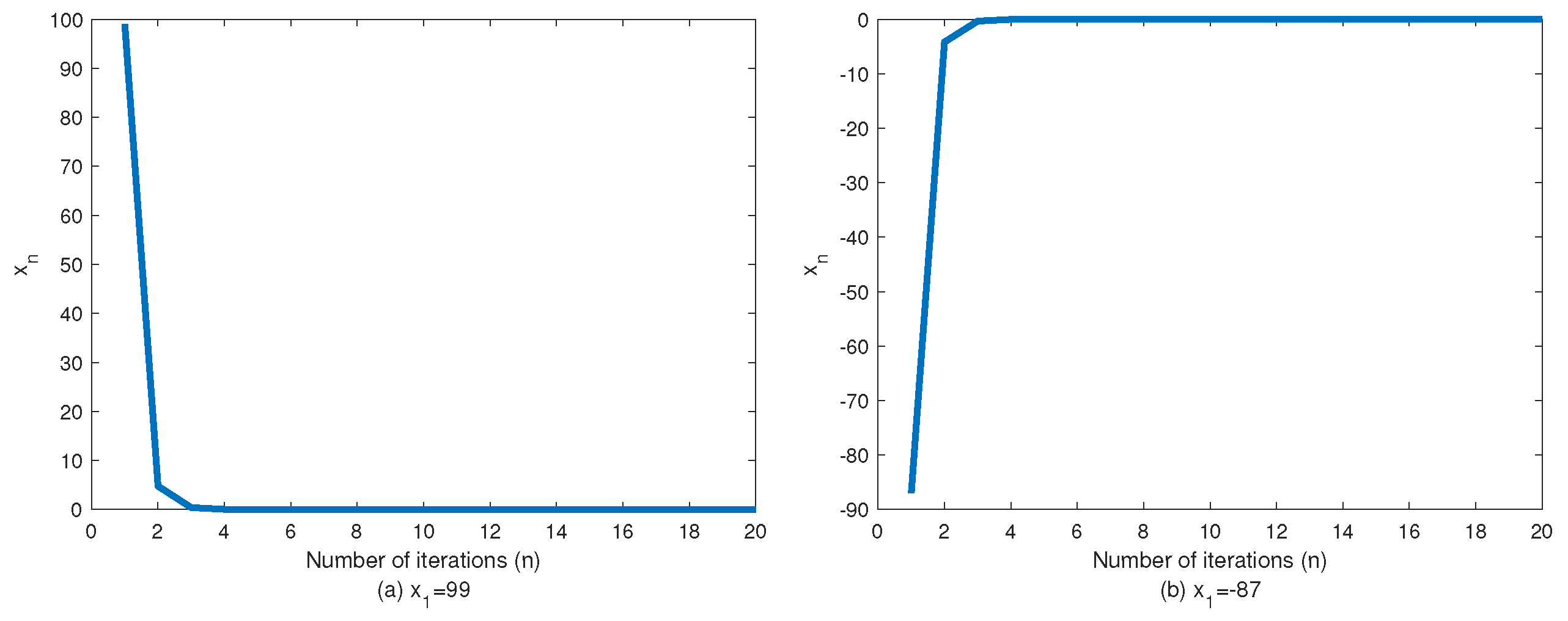
Example 1. 

Let $C=[-100,100]\subset H=\mathbb{R}$ and define $\varphi (x,y)=-8x^2+3xy+5y^2$. It is easy to verify that ϕ satisfies the conditions $\left(A_1\right)$–$\left(A_4\right)$. First, we deduce a formula for $Q_r\left(x\right)$. For any $y\in [-100,100]$ and $r>0$,

$$\begin{array}{cc}\hfill & \varphi (z,y)+{\displaystyle \frac{1}{r}}⟨y-z,z-x⟩\ge 0\iff \hfill \\ \hfill & 5r{y}^2+((1+3r)z-x)y+xz-(1+8r)z^2\ge 0.\hfill \end{array}$$

Set $G\left(y\right)=5r{y}^2+((1+3r)z-x)y+xz-(1+8r)z^2$. Then, $G\left(y\right)$ is a quadratic function of y with coefficients

$$\begin{array}{c}\hfill a:=5r,b:=((1+3r)z-x),c:=xz-(1+8r)z^2.\end{array}$$

Therefore, $z={\displaystyle \frac{x}{13r+1}}$, which yields $Q_r\left(x\right)={\displaystyle \frac{x}{13r+1}}$. So, from Lemma 3, we obtain $EP\left(\varphi \right)=\left\{0\right\}$. Let ${\alpha }_n={\displaystyle \frac{1}{5n}},{\lambda }_n={\displaystyle \frac{n+1}{48n}},{\mu }_n={\displaystyle \frac{1}{48n}},r_n={\displaystyle \frac{n}{2n-1}},s_n={\displaystyle \frac{1}{n}}$, and $T_{n}x={\displaystyle \frac{x}{n}}$ for all $n\in \mathbb{N}$. Suppose $Ax=3x$ with $\kappa =4$, $Fx={\displaystyle \frac{1}{4}}x$, $L={\displaystyle \frac{1}{2}}$, and $\eta ={\displaystyle \frac{1}{5}}$. Hence, $\Gamma ={\cap }_{n=1}^{\infty }F\left(T_n\right)\cap EP\left(\varphi \right)\cap VI(A,C)=\left\{0\right\}$. Then, from Theorem 1, the sequence $\left\{x_n\right\}$, generated iteratively by

$$\begin{array}{c}\hfill \left\{\begin{array}{c}{u}_n=Q_{r_n}{x}_n={\displaystyle \frac{2n-1}{15n-1}}{x}_n,\hfill \\ y_n=P_C(u_n-{\mu }_{n}A{u}_n)={\displaystyle \frac{16n-1}{16n}}{u}_n,\hfill \\ z_n=P_C(y_n-{\lambda }_{n}A{y}_n)={\displaystyle \frac{15n-1}{16n}}{y}_n,\hfill \\ v_n=P_C(u_n-{\lambda }_{n}A{z}_n)=u_n-({\displaystyle \frac{n+1}{16n}})z_n,\hfill \\ x_{n+1}=(1-{\alpha }_n)w_n+{\alpha }_n{T}_n{w}_n={\displaystyle \frac{20n^3-9n^2+5n-1}{20n^3}}{v}_n,\hfill \end{array}\right.\end{array}$$

converges strongly to the unique solution 0 of VIP (10).

In the following, we provide numerical results for two suitable initial points.

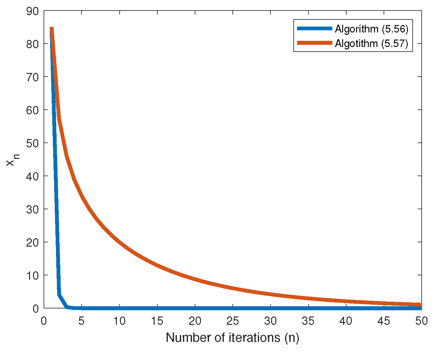
Now, we will compare the effectiveness of our algorithm with algorithm (9) via a numerical example.

Example 2. 

Let all the assumptions of Example 1 hold except the mappings $T_{n}x=Tx=x$ for all $n\in \mathbb{N}$. First, suppose the sequence $\left\{x_n\right\}$ is generated by (27). Then, the scheme (27) can be simplified as

$$\begin{array}{c}\hfill \left\{\begin{array}{c}{u}_n=Q_{r_n}{x}_n={\displaystyle \frac{2n-1}{15n-1}}{x}_n,\hfill \\ y_n=P_C(u_n-{\mu }_{n}A{u}_n)={\displaystyle \frac{16n-1}{16n}}{u}_n,\hfill \\ z_n=P_C(y_n-{\lambda }_{n}A{y}_n)={\displaystyle \frac{15n-1}{16n}}{y}_n,\hfill \\ v_n=P_C(u_n-{\lambda }_{n}A{z}_n)=u_n-({\displaystyle \frac{n+1}{16n}})z_n,\hfill \\ x_{n+1}=(1-{\alpha }_n)w_n+{\alpha }_n{T}_n{w}_n={\displaystyle \frac{4n-1}{4n}}{v}_n.\hfill \end{array}\right.\end{array}$$

(54)

Therefore, the sequence $\left\{x_n\right\}$ converges strongly to 0 by Theorem 1. Next, let the sequence $\left\{x_n\right\}$ be generated by (9). Then, the scheme (9) can be simplified as

$$\begin{array}{c}\hfill \left\{\begin{array}{c}{y}_n=P_C(x_n-{\mu }_{n}A{x}_n)={\displaystyle \frac{16n-1}{16n}}{x}_n,\hfill \\ z_n=P_C(y_n-{\lambda }_{n}A{y}_n)={\displaystyle \frac{15n-1}{16n}}{y}_n,\hfill \\ v_n=P_C(x_n-{\lambda }_{n}A{z}_n)=x_n-({\displaystyle \frac{n+1}{16n}})z_n,\hfill \\ x_{n+1}=(1-{\alpha }_n)w_n+{\alpha }_{n}T{w}_n={\displaystyle \frac{4n-1}{4n}}{v}_n.\hfill \end{array}\right.\end{array}$$

(55)

Therefore, the sequence $\left\{x_n\right\}$ converges strongly to 0 by Theorem 1.

Next, the numerical comparison of algorithms (54) and (55) is provided.

Table 1 and Table 2 and Figure 1 and Figure 2 show that the sequence $\left\{x_n\right\}$ generated by the above algorithms converges to 0.

Table 1. The values of the sequence $\left\{x_n\right\}$ for Algorithm (27).

n	${\mathit{x}}_{\mathit{n}}$	${\mathit{x}}_{\mathit{n}}$
1	99	−87
2	4.7597	−4.1828
3	0.37561	−0.33008
4	0.034591	−0.030398
5	0.0034407	−0.0030236
⋮	⋮	⋮
16	1.3236$\times {10}^{-13}$	$-1.1632\times {10}^{-13}$
17	$1.5671\times {10}^{-14}$	$-1.3771\times {10}^{-14}$
18	$1.8617\times {10}^{-15}$	$-1.636\times {10}^{-15}$
19	$2.2184\times {10}^{-16}$	$-1.9495\times {10}^{-16}$
20	$2.6507\times {10}^{-17}$	$-2.3294\times {10}^{-17}$

Numerical results for $x_1=99$ and $x_1=-87$.

Table 2. Comparison between Algorithm (54) and Algorithm (55).

n	${\mathit{x}}_{\mathit{n}}$ for (54)	${\mathit{x}}_{\mathit{n}}$ for (55)
1	85	85
2	4.0867	57.213
3	0.33947	1.0035
4	0.032716	38.963
5	0.003381	33.938
⋮	⋮	⋮
24	$7.309\times {10}^{-21}$	6.4915
25	$8.8944\times {10}^{-22}$	6.0339
26	$1.0837\times {10}^{-22}$	5.6115
27	$1.322\times {10}^{-23}$	5.221
28	$1.6143\times {10}^{-24}$	4.8599
⋮	⋮	⋮
46	$6.6475\times {10}^{-41}$	$1.4058$
47	$8.2107\times {10}^{-42}$	$1.3147$
48	$1.0145\times {10}^{-42}$	$1.2297$
49	$1.2539\times {10}^{-43}$	$1.1503$
50	$1.5503\times {10}^{-44}$	$1.0762$

Numerical results for $x_1=85$.

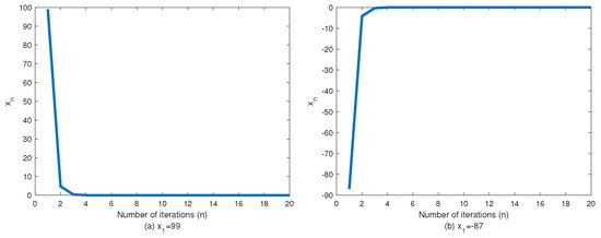
Figure 1. The convergence of $\left\{x_n\right\}$ with different initial values $x_1$.

Figure 2. Comparison between Algorithm (54) and Algorithm (55).

Remark 4. 

Table 2 shows that the convergent rate of iterative algorithm (27) is faster than that of iterative algorithm (9) of Hieu et al.

References

- Blum, E.; Oettli, W. From optimization and variatinal inequalities to equilibrium problems. Math. Stud. 1994, 63, 123–145. [Google Scholar]
- Daniele, P.; Giannessi, F.; Mougeri, A. (Eds.) Equilibrium Problems and Variational Models. Nonconvex Optimization and Its Application; Kluwer Academic Publications: Norwell, Australia, 2003; Volume 68. [Google Scholar]
- Sababe, S.H.; Yazdi, M. A hybrid viscosity approximation method for a common solution of a general system of variational inequalities, an equilibrium problem, and fixed point problems. J. Comput. Math. 2023, 41, 153–172. [Google Scholar]
- Hieu, D.V. An extension of hybrid method without extrapolation step to equilibrium problems. J. Ind. Manag. Optim. 2017, 13, 1723–1741. [Google Scholar] [CrossRef]
- Khuangsatung, W.; Kangtunyakarn, A. Iterative approximation method for various nonlinear mappings and equilibrium problems with numerical example. Rev. Real Acad. Cienc. Exactas Físicas Nat. Ser. A Mat. 2017, 111, 65–88. [Google Scholar] [CrossRef]
- Migot, T.; Cojocaru, M.-G. A parametrized variational inequality approach to track the solution set of a generalized nash equilibrium problem. Eur. J. Oper. Res. 2020, 283, 1136–1147. [Google Scholar] [CrossRef]
- Moudafi, A. Second order differential proximal methods for equilibrium problems. J. Inequal. Pure Appl. Math. 2003, 4, 1–7. [Google Scholar]
- Munkong, J.; Dinh, B.V.; Ungchittrakool, K. An inertial multi-step algorithm for solving equilibrium problems. J. Nonlinear Convex Anal. 2020, 21, 1981–1993. [Google Scholar]
- Wang, S.; Hu, C.; Chia, G. Strong convergence of a new composite iterative method for equilibrium problems and fixed point problems. Appl. Math. Comput. 2010, 215, 3891–3898. [Google Scholar] [CrossRef]
- Yazdi, M.; Hashemi Sababe, S. A new extragradient method for equilibrium, split feasibility and fixed point problems. J. Nonlinear Convex Anal. 2021, 22, 759–773. [Google Scholar]
- Yazdi, M.; Hashemi Sababe, S. Strong convergence theorem for a general system of variational inequalities, equilibrium problems, and fixed point problems. Fixed Point Theory 2022, 23, 763–778. [Google Scholar] [CrossRef]
- Yazdi, M.; Sababe, S.H. On a new iterative method for solving equilibrium problems and fixed point problems. Fixed Point Theory 2024, 25, 419–434. [Google Scholar] [CrossRef]
- Yao, Y.; Postolache, M.; Yao, C. An iterative algorithm for solving the generalized variational inequalities and fixed points problems. Mathematics 2019, 7, 61. [Google Scholar] [CrossRef]
- Hartman, P.; Stampacchia, G. On some non-linear elliptic differential-functional equation. Acta Math. 1966, 115, 271–310. [Google Scholar] [CrossRef]
- Korpelevich, G.M. The extragradient method for finding saddle points and other problems. Ekon. Mat. Metod. 1976, 12, 747–756. [Google Scholar]
- Censor, Y.; Gibali, A.; Reich, S. The subgradient extragradient method for solving variational inequalities in Hilbert space. J. Optim. Theory Appl. 2011, 148, 318–335. [Google Scholar] [CrossRef]
- Nadezhkina, N.; Takahashi, W. Weak convergence theorem by an extragradient method for nonexpansive mappings and monotone mappings. J. Optim. Theory Appl. 2006, 128, 191–201. [Google Scholar] [CrossRef]
- Maingé, P.E. A hybrid extragradient-viscosity method for monotone operators and fixed point problems. SIAM J. Control Optim. 2008, 47, 1499–1515. [Google Scholar] [CrossRef]
- Takahashi, S.; Toyoda, M. Weak convergence theorems for nonexpansive mappings and monotone mappings. J. Optim. Theory Appl. 2003, 118, 417–428. [Google Scholar] [CrossRef]
- Zeng, L.C.; Yao, J.C. Strong convergence theorem by an extragradient method for fixed point problems and variational inequality problems. Taiwan. J. Math. 2006, 10, 1293–1303. [Google Scholar] [CrossRef]
- Censor, Y.; Gibali, A.; Reich, S. Strong convergence of subgradient extragradient methods for the variational inequality problem in Hilbert space. Optim. Methods Softw. 2011, 26, 827–845. [Google Scholar] [CrossRef]
- Combettes, P.I.; Hirstoaga, S.A. Equilibrium programming in Hilbert spaces. J. Nonlinear Convex Anal. 2005, 6, 117–136. [Google Scholar]
- Yamada, I. The Hybrid Steepest Descent Method for the Variational Inequality Problem over the Intersection of Fixed Point Sets of Nonexpansive Mappings. In: Inherently Parallel Algorithms for Feasibility and Optimization and Their Applications. Stud. Comput. Math. 2004, 8, 473–504. [Google Scholar]
- Rockafellar, R.T. On the maximality of sums of nonlinear monotone operators. Trans. Am. Math. Soc. 1970, 149, 75–88. [Google Scholar] [CrossRef]
- Aoyama, K.; Kimura, Y.; Takahashi, W.; Toyoda, M. Approximation of common fixed points of a countable family of nonexpansive mappings in a Banach space. Nonlinear Anal. 2007, 67, 2350–2360. [Google Scholar] [CrossRef]
- Hieu, D.V.; Son, D.X.; Anh, P.K.; Muu, L.D. A two-step extragradient-viscosity method for variational inequalities and fixed point problems. Acta Math. Vietnam. 2019, 44, 531–552. [Google Scholar] [CrossRef]
- O’Hara, J.G.; Pillay, P.; Xu, H.K. Iterative approaches to convex feasibility problems in Banach spaces. Nonlinear Anal. 2006, 64, 2022–2042. [Google Scholar] [CrossRef]
- Shimoji, K.; Takahashi, W. Strong convergence to common fixed points of infinite nonexpansive mappings and applications. Taiwan. J. Math. 2001, 5, 387–404. [Google Scholar] [CrossRef]
Disclaimer/Publisher’s Note: The statements, opinions and data contained in all publications are solely those of the individual author(s) and contributor(s) and not of MDPI and/or the editor(s). MDPI and/or the editor(s) disclaim responsibility for any injury to people or property resulting from any ideas, methods, instructions or products referred to in the content. |
© 2024 by the authors. Licensee MDPI, Basel, Switzerland. This article is an open access article distributed under the terms and conditions of the Creative Commons Attribution (CC BY) license (https://creativecommons.org/licenses/by/4.0/).