Mechanical and Civil Engineering Optimization with a Very Simple Hybrid Grey Wolf—JAYA Metaheuristic Optimizer

Abstract

Metaheuristic algorithms (MAs) now are the standard in engineering optimization. Progress in computing power has favored the development of new MAs and improved versions of existing methods and hybrid MAs. However, most MAs (especially hybrid algorithms) have very complicated formulations. The present study demonstrated that it is possible to build a very simple hybrid metaheuristic algorithm combining basic versions of classical MAs, and including very simple modifications in the optimization formulation to maximize computational efficiency. The very simple hybrid metaheuristic algorithm (SHGWJA) developed here combines two classical optimization methods, namely the grey wolf optimizer (GWO) and JAYA, that are widely used in engineering problems and continue to attract the attention of the scientific community. SHGWJA overcame the limitations of GWO and JAYA in the exploitation phase using simple elitist strategies. The proposed SHGWJA was tested very successfully in seven “real-world” engineering optimization problems taken from various fields, such as civil engineering, aeronautical engineering, mechanical engineering (included in the CEC 2020 test suite on real-world constrained optimization problems) and robotics; these problems include up to 14 optimization variables and 721 nonlinear constraints. Two representative mathematical optimization problems (i.e., Rosenbrock and Rastrigin functions) including up to 1000 variables were also solved. Remarkably, SHGWJA always outperformed or was very competitive with other state-of-the-art MAs, including CEC competition winners and high-performance methods in all test cases. In fact, SHGWJA always found the global optimum or a best cost at most 0.0121% larger than the target optimum. Furthermore, SHGWJA was very robust: (i) in most cases, SHGWJA obtained a 0 or near-0 standard deviation and all optimization runs practically converged to the target optimum solution; (ii) standard deviation on optimized cost was at most 0.0876% of the best design; (iii) the standard deviation on function evaluations was at most 35% of the average computational cost. Last, SHGWJA always ranked 1st or 2nd for average computational speed and its fastest optimization runs outperformed or were highly competitive with their counterpart recorded for the best MAs.

1. Introduction

Metaheuristic algorithms (MAs) nowadays represent the standard approach to complex engineering optimization problems. The popularity of these algorithms is demonstrated by the wide variety of applications of MAs to various fields of science, engineering and technology. For example, some areas that can be mentioned include static and dynamic structural optimization [1,2], mechanical characterization of materials and structural identification (also including damage identification) [3,4,5], vehicle routing optimization [6], optimization of solar devices [7], forest fire mapping [8], urban water demand [9], 3D printing process optimization [10], identification of COVID-19 infection and cancer classification [11,12] image processing including feature extraction/selection [13].

Unlike gradient-based optimizers, MAs are stochastic algorithms that do not use gradient information to perturb design variables. In metaheuristic optimization, new trial solutions are randomly generated according to the inspiring principle of the selected algorithm. The trial solutions generated in each iteration attempt to improve the best record obtained so far. Exploration and exploitation are the two typical phases of metaheuristic search. In exploration, optimization variables are perturbed to a great extent to try to quickly identify the best regions of the design space, while exploitation performs local searches in a set of selected neighborhoods of the most promising solutions. Exploration governs the optimization search in the early iterations, while exploitation dominates as soon as the optimizer converges toward the global optimum.

Several classifications of MAs have been proposed in the literature. The first distinction is between single-solution algorithms where the optimizer updates the position of only one search agent and population-based algorithms where the optimizer operates on a population of candidate designs or search agents. However, the single-point search is limited to a few classical algorithms, such as simulated annealing and tabu search. Hence, the vast majority of MAs are population-based optimizers and their classification relies on the inspiring principle that drives the metaheuristic search. In this regard, MAs can be roughly divided into four categories: (i) evolutionary algorithms; (ii) science-based algorithms; (iii) human-based algorithms; (iv) swarm intelligence-based algorithms.

Evolutionary algorithms imitate evolution theory and evolutionary processes. Genetic algorithms (GAs) [14,15], differential evolution (DE) [16,17], evolutionary programming (EP) [18], evolution strategies (ES) [19], biogeography-based optimization (BBO) [20] and black widow optimization (BWO) [21] fall in this category. GAs and DE algorithms certainly are the most popular evolutionary algorithms. Their success is demonstrated by the about 7000 citations gathered by Refs. [14,15] and the 23,030 citations gathered by Ref. [16] in the Scopus database over about 35 years (a total of about 860 citations/year up to October 2024). GAs are based on Darwin’s concepts of natural selection. Selection, crossover and mutation operators are used for creating a new generation of designs starting from the parent designs stored in the previous iteration. DE includes four basic steps: random initialization of the population, mutation, recombination and selection. GAs and DE mainly differ in the selection process for generating the next generation of designs that will be stored in the population.

Science-based MAs mimic the laws of physics, chemistry, astronomy, astrophysics and mathematics. Simulated annealing (SA) [22,23], charged system search (CSS) [24], magnetic charged system search (MCSS) [25], ray optimization (RO) [26], colliding bodies optimization (CBO) [27], water evaporation optimization (WAO) [28], thermal exchange optimization (TEO) [29], equilibrium optimizer (EO) [30] and light spectrum optimizer (LSO) [31] are examples of physics-based MAs. Generally speaking, the above-mentioned methods tend to reach the equilibrium condition of mechanical, electro-magnetic or thermal systems under external perturbations. Optics-based methods such as RO and LSO utilize the concepts of refraction and dispersion of the light to set directions for exploring the search space. SA certainly is the most popular science-based metaheuristic algorithm considering the about 33,940 citations gathered by Ref. [22] in the Scopus database over 42 years (about 810 citations/year up to October 2024). SA mimics the annealing process in liquid or solid materials that reach the lowest energy level (a globally stable condition) as temperature decreases. The SA search strategy is rather simple: (i) a new trial solution replaces the current best record if it improves it; (ii) otherwise, a probabilistic criterion indicates if solution may improve the current best record in the next iteration. The “temperature” parameter is used in SA for computing probability and is progressively updated as the optimization progresses. SA has an inherent hill-climbing capacity given by search strategy (ii) that allows local minima to be eventually bypassed in the next iterations.

The artificial chemical reaction optimization algorithm (ACROA) [32], gas Brownian motion optimization (GBMO) [33] and Henry gas solubility optimization (HGSO) [34] are examples of chemistry-based MAs that also rely on important physics concepts such as Brownian motion and Henry’s law. ACROA simulates interactions between chemical reactants: the positions of search agents correspond to concentrations and potentials of reactants and they are no longer perturbed when no more reactions can take place. GBMO utilizes the law of motion, the Brownian motion of gasses and turbulent rotational motion to search for an optimal solution; search agents correspond to molecules and their performance is measured by their positions. HGSO mimics the state of equilibrium of a gas mixture in a liquid; search agents correspond to gasses and their optimal positions correspond to the equilibrium distribution of gasses in the mixture. HSGO is the most popular algorithm in this sub-category considering the about 780 citations (up to October 2024) gathered by Ref. [34] five years after its release.

Big bang–big crunch optimization (BB-BC) [35], the gravitational search algorithm (GSA) [36], galaxy-based search algorithm (GBSA) [37], black hole algorithm [38], astrophysics-inspired grey wolf algorithm [39] and supernova optimizer [40] are examples of MAs that mimic astronomical or astrophysical phenomena, such as the expansion (big bang)–contraction (big crunch) cycles that lead to the formation of new star–planetary systems, the spreading of stellar material following supernovae explosions, gravitational interactions between masses, interactions between black holes and starsand the movement of spiral galaxy arms, which also introduces the concept of elliptical orbit in the hunting process of wolves. GSA and BB-BC are the most popular algorithms in this sub-category, considering the about 6030 and 1280 citations, respectively, gathered by Refs. [35,36] in the Scopus database over almost two decades (a total of about 415 citations per year).

The sine cosine algorithm (SCA) [41], the Runge–Kutta optimizer (RUN) [42] and the arithmetic optimization algorithm (AOA) [43] are inspired by mathematics. In the SCA, candidate solutions fluctuate outwards or towards the best solution using a mathematical model based on sine and cosine functions. RUN combines a slope calculation scheme based on the Runge–Kutta method with an enhanced solution quality mechanism to increase the quality of trial designs. The AOA uses the four basic arithmetic operators (i.e., addition, subtraction, multiplication, division) to perturb the design variables of the current best record: in particular, multiplication and division drive the exploration phase, while addition and subtraction drive the exploitation phase. The AOA and RUN, respectively, were associated with about 1830 and 705 citations in Scopus after only 3 years from their release (a total of 845 citations/year). The SCA also achieved a considerable number of citations, about 4040 over 8 years with an average of about 505 citations/year up to October 2024.

Human-based MAs mimic human activities (e.g., talking, walking, playing, exploring new places/situations), behaviors (e.g., natural tendency to look for the best and avoid the worst, parental cares, teaching–learning, decision processes) and social sciences (including politics). Tabu search (TS) [44,45] was the first human-based MA and was developed about 40 years ago. TS is inspired by the ancestral concept that sacred things cannot be touched: hence, in the optimization process, local search is performed in the neighborhood of candidate solutions and solutions that do not improve the design are stored in a database so that the optimizer will not explore them and their neighborhoods further. Harmony search optimization (HS), which simulates the music improvisation process of jazz players [46,47], teaching–learning-based optimization (TLBO) [48], which simulates the teaching–learning mechanisms in a classroom and JAYA [49] using just one single equation to perturb the optimization variables to approach the current best record and escape from the worst candidate solution, are the most popular human-based MAs according to the number of citations reported in the Scopus database. In particular, TLBO achieved the highest average number of citations/year (about 300) and was cited in about 3920 papers since its release in 2011 as of October 2024. TLBO is followed by JAYA (about 250 citations/year for about 2000 citations gathered over 8 years and a huge number of variants and hybrid schemes) and HS (about 235 citations/year for 5450 citations over 23 years).

The learning process is an important source of inspiration in human-based MAs. This is demonstrated by the group teaching optimization algorithm (GTOA) [50], another teaching–learning-based algorithm where students (i.e., candidate solutions) are divided into groups according to defined rules; the teacher (current best record) adopts specific teaching methods to improve the knowledge of each group. The mother optimization algorithm (MOA) [51] mimics the human interaction between a mother and her children, simulating the mother’s care of her children in education, advice and upbringing. The preschool education optimization algorithm (PEOA) [52] simulates the phases of children’s preschool education, including (i) the gradual growth of the preschool teacher’s educational influence, (ii) individual knowledge development guided by the teacher and (iii) individual increases in knowledge and self-awareness. The learning cooking algorithm (LCA) [53] mimics the cooking learning activity of humans: children learn from their mothers, and children and mothers learn from a chef. The decision making behavior of humans is instead simulated by the collective decision optimization algorithm (CDOA) [54]: candidate solutions are generated by operators reproducing the different phases of the decision process that can be experience-based, others-based, group thinking-based, leader-based and innovation-based.

The imperialist competitive algorithm (ICA) [55] and the political optimizer (PO) [56] are based on politics, another important human activity. The ICA simulates the international relationships between countries: search agents represent countries that are categorized into colonies and imperialist states; powerful empires take possession of the former colonies of weak empires. Imperialistic competitions direct the search process toward the powerful imperialist or the optimum points. PO simulates all the major phases of politics (i.e., constituency allocation, party switching, election campaign, inter-party election and parliamentary affairs); the population is divided into political parties and constituencies, thus facilitating each candidate to update its position with respect to the party leader and the constituency winner. Learning behaviors of the politicians from the previous election are also accounted for in the optimization process.

Swarm intelligence-based algorithms reproduce the social/individual behavior of animals (insects, terrestrial animals, birds, and aquatic animals) in reproduction, food search, hunting, migration, etc. Most of the newly published MAs belong to this category. Particle swarm optimization (PSO) [57,58,59], developed in 1995, is the most popular MA overall: in particular, the seminal studies [57,58] gathered about 73,550 citations over 29 years in the Scopus database; the average citation rate is about 2535 articles/year, more than three times higher than for SA. PSO simulates interactions between individuals of bird/fish swarms. If one leading individual or a group of leaders see a desirable path to go through (for food, protection, etc.), the rest of swarm quickly follows the leader(s), even in the absence of direct connections. In the optimization process, a population of candidate designs (the particles) is generated. Particles move through the search space and their positions and velocities are updated based on the position of the leader(s) and the best positions of individual particles in each iteration until the optimum solution is reached.

Insect behavior has also inspired MA experts to a great extent. Ant system and colony optimization (AS, ACO) [60,61,62], which mimic the cooperative search technique in the foraging behavior of real-life ant colonies, artificial bee colony (ABC) [63], which simulates the nectar search carried out by bees, the firefly algorithm (FFA) [64,65], which simulates the social behavior of fireflies and their bioluminescent communication, and ant lion optimizer (ALO) [66], which simulates the hunting mechanism of ant lions, fall in this sub-category. The interest of the optimization community in insect-based MAs is confirmed by the high number of citations achieved by the algorithms mentioned above: about 11,320 for AS, ACO (i.e., 405 citations/year since 1996), 6335 for ABC (i.e., 370 citations/year since 2007), 2720 for ALO (i.e., about 300 citations/year since 2015) and 2895 for FFA (i.e., 207 citations/year since 2010) up to October 2024.

The grey wolf optimizer (GWO) [67], coyote optimization algorithm (COA) [68], snake optimizer (SO) [69] and snow leopard optimization algorithm (SLOA) [70] are MAs simulating the behavior of terrestrial animals. GWO and COA, respectively, mimic the hunting behavior of grey wolves and coyotes; SO mimics the mating behavior of snakes. SLOA is somehow more general than GWO, COA and SO as it perturbs optimization variables by means of operators simulating a wide variety of behaviors of a snow leopard, including travel routes and movement, hunting, reproduction and mortality. GWO is one of the most popular MAs considering the about 13,700 citations reported in Scopus since its release in 2014 up to October 2024: the average number of citations per year is about 1370, the second best amongst all MAs after PSO.

Cuckoo search (CS) [71,72], the crow search algorithm (CSA) [73], starling murmuration optimizer (SMO) [74] and bat algorithm (BA) [75,76] are MAs that mimic the behavior of birds and bats. While BA updates the population of candidate designs simulating the echolocation behavior of bats, CS reproduces the parasitic behavior of some cuckoo species that mix their eggs with those of other birds to guarantee the survival of their chicks. CSA simulates crows’ behavior concerning how they hide their excess food and retrieve it when the food is needed. SMO explores the search space by reproducing the flying behavior of starlings: exploration is carried out by means of the separating and diving search strategies while exploitation relies on the whirling strategy. CS is the most popular MA in this sub-category: the Scopus database reports about 8570 citations for Refs. [71,72] over 15 years with about 570 citations/year up to October 2024. CS is followed by BA (about 6030 citations for Refs. [75,76] since 2010 with about 430 citations/year) and CSA (about 1765 citations since 2016 with about 220 citations/year).

Among MAs inspired by aquatic animals, the following methods have to be mentioned. The dolphin echolocation algorithm (DE) [77] simulates the hunting strategy of dolphins based on the echolocation of prey. The whale optimization algorithm (WOA) [78] mimics the social behavior of humpback whales and, in particular, their bubble-net hunting strategy. The salp swarm algorithm (SSA) [79] simulates swarming and foraging behaviors of ocean salps. The marine predators algorithm (MPA) [80] updates design variables by simulating random walk movements (essentially Brownian motion and Lévy flight) of ocean predators. The giant trevally optimizer (GTO) [81] mimics hunting strategies of giant trevally marine fish, including Lévy flight movement. WOA is the most popular algorithm in this sub-category: the Scopus database reports about 9790 citations since 2016 with an average rate of about 1225 citations/year. WOA is followed by SSA, which gathered about 3920 citations since 2017 with about 560 citations/year, and by MPA, which gathered about 1600 citations since 2020 with about 400 citations/year up to October 2024.

A large number of improved/enhanced variants for existing MAs, hybrid algorithms combining MAs with gradient-based optimizers, and hybrid algorithms combining two or more MAs have been developed by optimization experts (see, for example, Refs. [82,83,84,85,86,87,88,89,90,91,92,93,94,95,96,97,98,99,100,101,102], published in the last two decades). High-performance MAs were often selected as component algorithms in developing hybrid formulations. The common denominator of all those studies was to find the best balance between exploration and exploitation phases that hopefully resulted in the following: (i) the optimizer’s ability to avoid local minima (i.e., hill-climbing capability, especially for algorithms including SA-based operators), keeping the diversity in the population, and avoiding stagnation and premature convergence to false optima; (ii) a reduction in the number of function evaluations (structural analyses, analyses) required in the optimization process; (iii) high robustness in terms of low dispersion on optimized cost function values; (iv) a reduction in the number of internal parameters as well as in the level of heuristics entailed by the search process. In general, these tasks were accomplished by (i) combining highly explorative methods with highly exploitative methods; (ii) forcing the optimizer to switch again to exploration if the exploitation phase started prematurely or the design did not improve for a certain number of iterations in the exploitation phase; (iii) introducing new perturbation strategies (for example, chaotic perturbation of the design; mutation operators to avoid stagnation and increase the diversity of the population; Lévy flight/movements in swarm-based methods, etc.) for optimization variables tailored to the specific MA under consideration.

Continuous increases in computing power have greatly favored the development of new metaheuristic algorithms (including enhanced variants and hybrid formulations). However, some aspects should carefully be considered in metaheuristic optimization: (i) according to the No Free Lunch theorem [103,104], no metaheuristic algorithm can always outperform all other MAs in all optimization problems; (ii) MAs often require a very large number of function evaluations (analyses) for completing the optimization process, even 1–2 orders of magnitude higher than their classical gradient-based optimizer counterparts; (iii) the easiness of implementation, which is typically underlined as a definite strength point of Mas, is very often nullified by the complexity of algorithmic variants or hybrid algorithms combining multiple methods; and (iv) sophisticated MA formulations often include many internal parameters that may be difficult to tune.

It should be noted that newly developed MAs often add very little to the optimization field and their appeal quickly vanishes just a few years after their release. This is confirmed by the literature survey presented in this introduction. The “classical” MAs developed prior to 2014, such as GA, DE, SA, PSO, ACO, CS, BA, HS, GSA, BBBC and GWO, gathered a much higher number of citations/year (up to 2535 until October 2024) than the MAs developed in 2015-2024, except for WOA, SCA, AOA/RUN, SSA, MPA, ALO, JAYA and CSA (up to 1225 citations/year). For this reason, the present study focused on improving available MAs rather than formulating a new MA from scratch. The main goal was to prove that a very efficient hybrid metaheuristic algorithm can be built by simply combining the basic formulations of two well-established MAs without complicating the formulation of the hybrid optimizer both in terms of number of strategies/operators used for perturbing the design variables and number of internal parameters (including parameters that regulate the switching from one optimizer to another).

In view of the arguments above, a very simple hybrid metaheuristic algorithm (SHGWJA, where the acronym stands for Simple Hybrid Grey Wolf JAYA) able to solve engineering optimization problems with less computational effort than the other currently available MAs was developed by combining two classical population-based MAs, namely the Grey Wolf Optimizer (GWO) and the Jaya Algorithm (JAYA). GWO and JAYA were selected in this study as the component algorithms of the new optimizer SHGWJA because of their simple formulations without internal parameters, and in view of the high interest of metaheuristic optimization experts in these two methods, proven by the various applications and many algorithmic variants documented in the literature. These motivations are detailed as follows.

(1)

GWO, originally developed by Mirjalili et al. [67] in 2014, is the second most cited metaheuristic algorithm after PSO in terms of citations/year. However, GWO has a much simpler formulation than PSO and, unlike PSO, does not require any setting of internal parameters. GWO mimics the hierarchy of leadership and group hunting of the grey wolves in nature: the optimization search is driven by the three best individuals that catch the prey and attract the rest of the hunters. Applications of GWO to various fields of science, engineering and technology are reviewed in Refs. [105,106].

(2)

JAYA, originally developed by Rao [49] in 2016, is one of the most cited MAs released in the last decade. It utilizes the most straightforward search scheme ever presented in the metaheuristic optimization literature for a population-based MA: to approach the population’s best solution and move away from the worst solution, thus achieving significant convergence capability. Hence, optimization variables are perturbed by JAYA using only one equation, thus minimizing the computational complexity of the search process. In spite of its inherent simplicity, JAYA is a powerful metaheuristic algorithm that has been proven able to efficiently solve a wide variety of optimization problems (see, for example, the reviews presented in [107,108]). An interesting argument made in [107] may explain JAYA’s versatility. JAYA combines the basic features of evolutionary algorithms, in terms of the fittest individual’s survivability (such a feature is, however, common to all population-based MAs), and swarm-based algorithms where the swarm normally follow the leader during the search for an optimal solution. This hybrid nature, in addition to the inherent algorithmic simplicity, makes JAYA an ideal candidate to be selected as a component of new hybrid metaheuristic algorithms.

(3)

Both GWO and JAYA do not have internal parameters that have to be set by the user, except the parameters common to all population-based MAs, such as population size and the limit on the number of optimization iterations.

(4)

Both algorithms have good exploration capabilities but have weaknesses in the exploitation phase. The challenge is to combine their exploration capabilities to directly approach the global optimum. Elitist strategies may facilitate the exploitation phase, which only has to focus on a limited number of potentially optimal solutions to be refined.

Here, GWO and JAYA were simply merged, and the JAYA perturbation strategy was applied to improve the positions of the leading wolves, thus avoiding the search stagnation that may occur in GWO if the three best individuals of the population remain the same for many iterations. The original formulations of GWO and JAYA combined into the hybrid SHGWJA algorithm were slightly modified to maximize the search capability of the new algorithm and reduce the number of function evaluations required by the GWO and JAYA engines. However, while algorithmic variants of GWO and JAYA (including hybrid optimizers) usually include specific operators/schemes to increase the diversity of the population or/and improve the exploitation capability (this, however, increases the computational complexity of the optimizer) [105,106,107,108], SHGWJA adopts a very straightforward elitist approach. In fact, SHGWJA always attempts to improve the current best design of the population regardless of having generated new trial solutions in the exploration phase or exploitation phase. Trial solutions that are unlikely to improve the current best record stored in the population are directly rejected without evaluating constraints. This allows SHGWJA to reduce the computational cost of the optimization process by always directing the search process towards the best regions of the search space, and eliminating any unnecessary exploitation of trial solutions that cannot improve the current best record.

The proposed SHGWJA was successfully tested in seven “real-world” engineering problems selected from civil engineering, mechanical engineering and robotics. The selected test problems, including up to 14 optimization variables and 721 nonlinear constraints, regarded: (i) shape optimization of a concrete gravity dam (volume minimization); (ii) optimal design of a tension/compression spring (weight minimization); (iii) optimal design of a welded beam (minimization of fabrication cost); (iv) optimal design of a pressure vessel (minimization of forming, material, and welding costs); (v) optimal design of an industrial refrigeration system; (vi) 2D path planning (minimization of trajectory length); (vii) mechanical characterization of a flat composite panel under axial compression (by matching experimental data and finite element simulations). Test problems (ii) through (v) were included in the CEC 2020 (IEEE Congress on Evolutionary Computing) test suite for constrained mechanical engineering problems. Example (vii) is a typical highly nonlinear inverse problem in the fields of aeronautical engineering and mechanics of materials. Besides the seven “real-world” engineering problems listed above, two classical mathematical optimization problems (i.e., Rosenbrock’s banana function and Rastrigin’s function) with up to 1000 variables were solved in this study to evaluate the scalability of the proposed algorithm.

For all test cases, the optimization results obtained by SHGWJA were compared with those quoted in the literature for the best-performing algorithms. SHGWJA was compared with at least 10 other MAs, each of which had been reported in the literature to have outperformed in turn up to 35 other MAs. Comparisons with high performance algorithms and CEC competitions winners such as LSHADE and IMODE variants as well as with other MAs that were reported to outperform CEC winners (i.e., MPA and GTO among others) also are presented in the article.

The rest of the article is structured as follows. Section 2 recalls formulations of GWO and JAYA, while Section 3 describes the new hybrid optimization algorithm SHGWJA developed in this research. Test problems and implementation details are presented in Section 4, while optimization results are presented and discussed in Section 5. In the last section, the main findings are summarized, and directions of future research are outlined.

2. The GWO and JAYA Algorithms

2.1. The GWO Algorithm

The grey wolf optimization (GWO) algorithm reproduces the leadership hierarchy and hunting mechanism of grey wolves in nature [67]. GWO simulates the leadership hierarchy by defining four types of grey wolves, namely α, β, δ and ω. The hunting mechanism is simulated by different operations corresponding to searching for prey, encircling prey and attacking prey. The α wolf is the group leader and makes decisions regarding hunting, sleeping place, time to wake, etc. The β wolf helps the α in decision making or other pack activities. The lowest-ranking grey wolf is the ω, which must submit to dominant wolves. Delta wolves (scouts, sentinels, elders, hunters and caretakers) must submit to α and β wolves, but they dominate the ω wolves. Alpha, beta, and delta wolves estimate the position of the prey, and other wolves update their positions randomly around the prey.

GWO starts with defining the population of N_POP wolves covering the search space. The best three individuals stored in the population are ranked as α, β and δ. The rest of the population is ranked as ω. Prey is encircled by wolves during the hunt. This behavior is mathematically described as follows:

$$\stackrel{\rightharpoonup }{D}=\left|\overrightarrow{C}·\overrightarrow{X_p}\right|-\overrightarrow{X_{it}}$$

(1)

$$\overrightarrow{X_{it+1}}=\overrightarrow{X_p}-\overrightarrow{A}·\overrightarrow{D}$$

(2)

where it refers to the current iteration, $\overrightarrow{A}$ and $\overrightarrow{C}$ are coefficient vectors, $\overrightarrow{X_p}$ is the position vector of the prey and $\overrightarrow{X_{it}}$ is the generic grey wolf (i.e., search agent) included in the population. The “$·$” notation denotes the term by term multiplication between vectors which results in another vector.

Vectors $\overrightarrow{A}$ and $\overrightarrow{C}$ are defined as follows:

$$\stackrel{\rightharpoonup }{A}=2\overrightarrow{a}·\overrightarrow{r_1}-\overrightarrow{a}$$

(3)

$$\stackrel{\rightharpoonup }{C}=2\overrightarrow{r_2}$$

(4)

where the components of the $\overrightarrow{a}$ vector decrease linearly from 2 to 0 as the optimization progresses, and $\overrightarrow{r_1},\overrightarrow{r_2}$ are random vectors in the [0, 1] interval.

In the hunting phase, grey wolves recognize their prey’s location and encircle it. However, in an optimization search, the location of the optimum (prey) is usually not known a priori. To simulate wolves’ hunting behavior, GWO assumes that the three best search agents corresponding to α, β and δ wolves have a better knowledge of the potential prey’s location (i.e., the target optimum). Hence, all other agents must update their positions based on the positions of the best three search agents, $\overrightarrow{X_{\alpha }}$, $\overrightarrow{X_{\beta }}$ and $\overrightarrow{X_{\delta }}$. Such a task is accomplished by the following equations for the generic solution $\overrightarrow{X_{it}}$ included in the population:

$$\left\{\begin{array}{c}\stackrel{\rightharpoonup }{D_{\alpha }}=\left|\overrightarrow{C_1}·\overrightarrow{X_{\alpha }}\right|-\overrightarrow{X_{it}}\\ \stackrel{\rightharpoonup }{D_{\beta }}=\left|\overrightarrow{C_2}·\overrightarrow{X_{\beta }}\right|-\overrightarrow{X_{it}}\\ \stackrel{\rightharpoonup }{D_{\delta }}=\left|\overrightarrow{C_3}·\overrightarrow{X_{\delta }}\right|-\overrightarrow{X_{it}}\end{array}\right.$$

(5)

$$\left\{\begin{array}{c}\stackrel{\rightharpoonup }{X_1}=\overrightarrow{X_{\alpha }}-\overrightarrow{A_1}·\overrightarrow{ D_{\alpha }}\\ \stackrel{\rightharpoonup }{X_2}=\overrightarrow{X_{\beta }}-\overrightarrow{A_2}·\overrightarrow{ D_{\beta }}\\ \stackrel{\rightharpoonup }{X_3}=\overrightarrow{X_{\delta }}-\overrightarrow{A_3}·\overrightarrow{D_{\delta }}\end{array}\right.$$

(6)

$$\stackrel{\rightharpoonup }{X_{it+1}}={\displaystyle \frac{\stackrel{\rightharpoonup }{X_1}+\stackrel{\rightharpoonup }{X_2}+\stackrel{\rightharpoonup }{X_3}}{3}}$$

(7)

where the vectors $\stackrel{\rightharpoonup }{X_1}, \stackrel{\rightharpoonup }{X_2} \mathrm{and} \stackrel{\rightharpoonup }{X_3}$ are defined for each individual $\stackrel{\rightharpoonup }{X_i}$ of the population.

Equations (5) through (7) are utilized to update the positions of all search agents. The new population is ordered with respect to penalized cost function values to update the positions $\overrightarrow{X_{\alpha }}$, $\overrightarrow{X_{\beta }}$ and $\overrightarrow{X_{\delta }}$. The prey’s position corresponds to the current best record. The process is repeated until the limit number of iterations or function evaluations defined by the user is completed.

In summary, in the optimization iterations, α, β and δ wolves estimate the prey’s position (target optimal solution corresponding to the current best record) and each search agent updates its distance from prey. The a parameter decreases from 2 to 0 in order to govern the exploration phase and exploitation phase, respectively. Candidate solutions tend to diverge from prey and search for another prey in the exploration phase when $\Vert \overrightarrow{A}\Vert$ > 1, while they converge towards the prey in the exploitation phase when $\Vert \overrightarrow{A}\Vert$ < 1.

The main drawbacks of GWO are premature convergence and low diversity because the population is moved towards only the three best search agents, the wolves α, β and δ. For this reason, Nadimi-Shahraki et al. [105] developed the gaze cues learning-based grey wolf optimizer (GGWO) algorithm. GGWO implemented new search strategies based on other typical behaviors of grey wolves, such as the gaze cues learning. Wolves may direct their attention towards some target simply by following the sight of other wolves that found the target sufficiently interesting. In order to implement this mechanism in the optimization search, GGWO defined three candidate solutions for updating each design $\stackrel{\rightharpoonup }{X_i}$ of the population: (i) the $\overrightarrow{X_{i-GWO}}$ solution obtained with classical GWO, Equation (7); (ii) the $\overrightarrow{X_{i-NGCL}}$ solution generated with the neighbor gaze cues learning (NGCL) search strategy, where $\stackrel{\rightharpoonup }{X_i}$ is updated considering the alpha wolf $\overrightarrow{X_{\alpha }}$, and the neighborhood of $\stackrel{\rightharpoonup }{X_i}$ formed by two wolves ranked immediately below $\stackrel{\rightharpoonup }{X_i}$ and two wolves ranked immediately above $\stackrel{\rightharpoonup }{X_i}$; (iii) the $\overrightarrow{X_{i-RGCL}}$ solution generated with the random gaze cues learning (RGCL) search strategy where $\stackrel{\rightharpoonup }{X_i}$ is updated considering two randomly selected wolves from the population. The fitness values of the three candidate solutions $\overrightarrow{X_{i-GWO}}$, $\overrightarrow{X_{i-NGCL}}$ and $\overrightarrow{X_{i-RGCL}}$ are compared and the best-fitted amongst the three individuals is provisionally set as the new $\stackrel{\rightharpoonup }{X_i}$, which replaces the old $\stackrel{\rightharpoonup }{X_i}$ solution if it has a better fitness than the old $\stackrel{\rightharpoonup }{X_i}$.

Very recently, Tsai and Shi [106] proposed two GWO variants that correct the original formulation of GWO to remove causes of potential biases in the search process. The GWO–C1 variant does not use the $\overrightarrow{C}$ vector and the absolute value any more to compute the $\overrightarrow{D}$ vectors in Equation (5). Furthermore, in the GWO–C2 variant, Equation (6) is modified by replacing $\overrightarrow{X_{\alpha }}$, $\overrightarrow{X_{\beta }}$ and $\overrightarrow{X_{\delta }}$ with the current position $\overrightarrow{X_{it}}$. Both the GWO–C2 and GGWO algorithms were very competitive in solving CEC test suites but GGWO fits better in the present study because it was tested in [105] in real engineering problems.

2.2. The JAYA Algorithm

The JAYA method is the simplest metaheuristic algorithm ever presented in the optimization literature [49]. It only utilizes one equation to perturb the design and does not include any internal parameter besides population size N_POP and the limit on the number of iterations N_itermax. Let X_j,i,it be the jth optimization variable (j = 1,…, NDV) for the ith search agent (i = 1,…, N_POP) in the itth iteration. The X_j,i,it value is modified in the current iteration as follows:

$$X_{j,i,it}^{new}=X_{\mathrm{j},\mathrm{i},\mathrm{it}}+r_{1,\mathrm{j},\mathrm{it}}\left(X_{\mathrm{j},\mathrm{best},\mathrm{it}}-\left|X_{\mathrm{j},\mathrm{i},\mathrm{it}}\right|\right)-r_{2,\mathrm{j},\mathrm{it}}\left(X_{\mathrm{j},\mathrm{worst},\mathrm{it}}-\left|X_{\mathrm{j},\mathrm{i},\mathrm{it}}\right|\right)$$

(8)

where $X_{\mathrm{j},\mathrm{i},\mathrm{it}}^{\mathrm{new}}$ is the updated value of $X_{\mathrm{j},\mathrm{i},\mathrm{it}}$; $r_{1,\mathrm{j},\mathrm{it}}$ and $r_{2,\mathrm{j},\mathrm{it}}$, respectively, are two random numbers extracted from the [0, 1] interval for the jth variable; $X_{\mathrm{j},\mathrm{best},\mathrm{it}}$ and $X_{\mathrm{j},\mathrm{worst},\mathrm{it}}$, respectively, are the values of the jth variable for the best individual X_best,it and worst individual X_worst,it currently included in the population.

The term ${\mathrm{r}}_{1,\mathrm{j},\mathrm{it}}\left(X_{\mathrm{j},\mathrm{best},\mathrm{it}}-\left|X_{\mathrm{j},\mathrm{i},\mathrm{it}}\right|\right)$ describes JAYA’s ability to approach the best solution $\overrightarrow{X_{best,it}}$, while the term $-r_{2,\mathrm{j},\mathrm{it}}\left(X_{\mathrm{j},\mathrm{worst},\mathrm{it}}-\left|X_{\mathrm{j},\mathrm{i},\mathrm{it}}\right|\right)$ describes its ability to escape from the worst solution $\overrightarrow{X_{worst,it}}$. Random factors r₁ and r₂ allow the design space to be efficiently explored while the absolute value $\left|X_{\mathrm{j},\mathrm{i},\mathrm{it}}\right|$ in Equation (8) further enhances exploration [49]. It should be noted that using the absolute value $\left|X_{\mathrm{j},\mathrm{i},\mathrm{it}}\right|$ in Equation (8) does not affect the search process in real engineering problems because optimization variables can usually take only positive values. However, in mathematical optimization problems where variables may take optimal values of 0, using the absolute value $\left|X_{\mathrm{j},\mathrm{i},\mathrm{it}}\right|$ in Equation (8) actually limits the movements $\left(X_{\mathrm{j},\mathrm{best},\mathrm{it}}-\left|X_{\mathrm{j},\mathrm{i},\mathrm{it}}\right|\right)$ and $\left(X_{\mathrm{j},\mathrm{worst},\mathrm{it}}-\left|X_{\mathrm{j},\mathrm{i},\mathrm{it}}\right|\right)$, thus reducing biases in the convergence to zero values.

The new trial solution $\overrightarrow{{X_i}^{new}}$ defined by Equation (8) is compared with the previous solution $\overrightarrow{{X_i}^{pre}}$ in the population. If $\overrightarrow{{X_i}^{new}}$ is better than $\overrightarrow{{X_i}^{pre}}$, the population is updated by replacing $\overrightarrow{{X_i}^{pre}}$ with $\overrightarrow{{X_i}^{new}}$. This is reiterated until the limit number of iterations/function evaluations is reached. In most implementations, the computational cost of JAYA is N_POP × N_itermax function evaluations. JAYA variants [93,109] have tried to save computational cost by directly rejecting worse trial solutions than the search agents stored in the population; however, this strategy failed to find global optima in many structural optimization problems different from truss weight minimization. A similar approach was followed in [110]: the new trial solution $\overrightarrow{{X_i}^{new}}$ generated by the SJAYA variant replaces the $\overrightarrow{{X_i}^{pre}}$ solution that is being currently perturbed not only if it improves $\overrightarrow{{X_i}^{pre}}$ but also if it has the same cost (or penalized cost in constrained optimization).

Improving the balance of exploration and exploitation in JAYA is the most important concern of optimization experts. In this regard, Rao and Saroj [111] implemented in their SAMP-JAYA algorithm an adaptive scheme to divide the population into m sub-populations. Subpopulations are independently updated and then merged. Their number is increased to (m + 1) if the best record $\overrightarrow{X_{best,it}}$ is improved in the current iteration or it is decreased to (m − 1) if $\overrightarrow{X_{best,it}}$ is not improved. In this way, exploration characterizes the search process if iterations are successful while exploitation is activated if the optimizer cannot find a better solution over the whole search space covered by the sub-populations.

In [98], JAYA was hybridized with the Rao-1 optimizer into the EHRJAYA algorithm. Optimization variables are perturbed with JAYA or Rao-1 schemes based on a probabilistic threshold. This allows for improving the population diversity and solving situations of insufficient exploration and exploitation that may occur if the same perturbation strategy is utilized throughout the optimization process. A self-adaptive classification learning strategy assigns the perturbation equation to each individual based on its rank in the population. Each perturbation equation includes coefficients that adaptively vary in the optimization process. Population is continuously reduced in size to facilitate a smooth transition from exploration to local exploitation.

Zhang et al. [112] developed the variant EJAYA, which uses population information more efficiently than classical JAYA to balance exploration and exploitation. EJAYA updates optimization variables considering the current best and worst solutions (like classical JAYA), the current mean solution (obtained by averaging the N_POP search agents of the population), and the historical solutions (a population of candidate solutions initially generated besides the standard population and probabilistically permuted in the optimization process). In EJAYA, local exploitation relies on defined upper and lower local attractors (weighted averages of best/worst and average solution), while global exploration is guided by the historical population.

Fuzzy clustering competitive learning, experience learning and Cauchy mutation mechanisms were recently included in the I-JAYA algorithm [113]. The fuzzy clustering competitive learning mechanism effectively utilizes population information, speeding up convergence. Experience learning allows for balancing between exploiting previously visited regions and exploring new regions of the search space. Cauchy mutation reduces the risk of being stuck in local optima by fine-tuning the quality of the current best solution.

3. The SHGJA Algorithm

The simple hybrid metaheuristic algorithm SHGWJA developed in this research combined the GWO and JAYA methods to improve search by means of elitist strategies. The new algorithm is very simple and efficiently explores the search space. This allows for limiting the number of function evaluations. The new algorithm is now described in detail. A population of N_POP candidate designs (i.e., wolves) is randomly generated as follows:

$$x_j^i=x_j^L+{{\rho }_j}^i \hspace{0.17em}(x_j^U-x_j^L) \left\{\begin{array}{c}j=1,\dots ,NDV\\ i=1,\dots ,N_{POP}\end{array}\right.$$

(9)

where NDV is the number of optimization variables; $x_j^L$ and $x_j^U$, respectively, are the lower and upper bounds of jth variable; ${{\rho }_j}^i$ is a random number extracted in the interval (0, 1).

Considering the classical statement of the optimization problem where the goal is to minimize the function W($\overrightarrow{X}$) of NDV variables (stored in the design vector $\overrightarrow{X}$), subjected to N_CON inequality/equality constraint functions of the form G_k($\overrightarrow{\mathrm{X}}$) ≤ 0, the penalized cost function W_p($\overrightarrow{X}$) is defined as follows:

$$W_p\left(\overrightarrow{X}\right)=W\left(\overrightarrow{X}\right)+p·\psi$$

(10)

where p is the penalty coefficient. The penalty function $\psi$ is defined as follows:

$$\psi ={\displaystyle \sum }_{k=1}^{N_{con}}{\left(\max \left(0,g_j\right)\right)}^2$$

(11)

The penalized cost function W_p($\overrightarrow{X}$) obviously coincides with the cost function W($\overrightarrow{X}$) if the trial solution $\overrightarrow{X}$ is feasible. Candidate solutions are sorted with respect to penalized cost function values: the current best record corresponds to the lowest value of $\psi$.

• Step 1. Generation of new trial designs with classical GWO

The best three search agents achieving the lowest penalized cost values are set as the wolves α, β and δ. Let $\overrightarrow{X_{\alpha }}$, $\overrightarrow{X_{\beta }}$ and $\overrightarrow{X_{\delta }}$ be the corresponding design vectors. It obviously holds that W_p($\overrightarrow{X_{\alpha }}$) < W_p($\overrightarrow{X_{\beta }}$) < W_p($\overrightarrow{X_{\delta }}$). The α wolf is also set as the current best record $\overrightarrow{X_{opt}}$ and the corresponding penalized cost function W_p($\overrightarrow{X_{\alpha }}$) is set as W_p,opt.

Each individual $\overrightarrow{X_i}$ of the population is provisionally updated with the classical GWO Equations (1) through (7). As in [67], the components of the $\overrightarrow{a}$ vector linearly decrease from 2 to 0 as the optimization goes by in SHGWJA. Let $\overrightarrow{X_{i,tr}}$ denote the new trial solution obtained by perturbing the generic individual $\overrightarrow{X_i}$ stored in the population in the previous iteration.

• Step 2. Evaluation and refinement of new trial designs: Elitist strategy and JAYA schemes

Each new trial design $\overrightarrow{X_{i,tr}}$ generated in Step 1 via classical GWO with Equations (1) through (7) is evaluated by SHGWJA using two new operators. In GWO implementations, each new design $\overrightarrow{X_{i,tr}}$ is compared with its counterpart solution $\overrightarrow{X_i}$ previously stored in the population. If the new design $\overrightarrow{X_{i,tr}}$ is better than the old design $\overrightarrow{X_i},$ it is stored in the updated population in the current iteration, replacing the old design. However, this task requires a new evaluation of the constraint functions for each new $\overrightarrow{X_{i,tr}}$.

In order to reduce the computational cost, SHGWJA implements an elitist strategy, retaining only the trial solutions that are likely to improve the current best record. Hence, SHGWJA initially compares only the cost function W($\overrightarrow{X_{i,tr}}$) of the new trial solution $\overrightarrow{X_{i,tr}}$ with 1.1 times the cost function W($\overrightarrow{X_{opt}}$) of the current best record. If the new trial design does not improve the current best record—i.e., if W($\overrightarrow{X_{i,tr}}$) > 1.1W($\overrightarrow{X_{opt}}$) holds— it is not necessary to process it further and the old design $\overrightarrow{X_i}$ is provisionally maintained also in the new population.

The 1.1W($\overrightarrow{X_{opt}}$) threshold has proven to be effective in all test problems solved in this study. Such a behavior may be explained in the following way. In the exploration phase, the optimizer assigns large movements to design variables and the probability to improve design is high: hence, the W($\overrightarrow{X_{i,tr}}$) > 1.1W($\overrightarrow{X_{opt}}$) scenario will not be likely to occur. In the exploitation phase, the optimizer should bypass local minima to find the global optimum: like SA, the optimizer may accept candidate solutions slightly worse than $\overrightarrow{X_{opt}}$. Looking at the probabilistic acceptance/rejection criterion used by advanced SA formulations [84,93], it can be seen that the threshold level of acceptance probability is 0.9 if the γ ratio between the cost function increment recorded for the trial solution $\overrightarrow{X_{i,tr}}$ with respect to the current best record $\overrightarrow{X_{opt}}$ and the annealing temperature T is 0.1; hence, the probability of provisionally accepting some design worse than $\overrightarrow{X_{opt}}$ and improving it in the next iterations is 90%. Since the initial value of the T temperature set in SA corresponds to the expected optimum cost (or the cost value of the current best record), it may be reasonably assumed that trial solutions up to 10% worse than $\overrightarrow{X_{opt}}$ would become better than $\overrightarrow{X_{opt}}$ in the next iterations.

However, the new design $\overrightarrow{X_{i,tr}}$ is generated by classical GWO to try to approach the position of the best three individuals, the wolves α, β and δ. To avoid stagnation, the $\overrightarrow{X_i}$ design is perturbed using a JAYA-based scheme if the classical GWO generation was unsuccessful and the trial solution $\overrightarrow{X_{i,tr}}$ did not satisfy the condition W($\overrightarrow{X_{i,tr}}$) ≤ 1.1W($\overrightarrow{X_{opt}}$). That is, the following holds:

$${\left(\overrightarrow{X_{i,tr}}\right)}^{\prime }=\overrightarrow{X_i}+\overrightarrow{{\lambda }_1} ·\left(\overrightarrow{X_{opt}}-\overrightarrow{X_i}\right)-\overrightarrow{{\lambda }_2} ·\left(\overrightarrow{X_{worst}}-\overrightarrow{X_i}\right)$$

(12)

If the classical GWO generation was successful and trial design $\overrightarrow{X_{i,tr}}$ satisfied the condition W($\overrightarrow{X_{i,tr}}$) ≤ 1.1W($\overrightarrow{X_{opt}}$), the JAYA scheme is applied directly to $\overrightarrow{X_{i,tr}}$ as follows:

$${\left(\overrightarrow{X_{i,tr}}\right)}^{\prime }=\overrightarrow{X_{i,tr}}+\overrightarrow{{\lambda }_1} ·\left(\overrightarrow{X_{opt}}-\overrightarrow{X_{i,tr}}\right)-\overrightarrow{{\lambda }_2} ·\left(\overrightarrow{X_{\delta }}-\overrightarrow{X_{i,tr}}\right)$$

(13)

In Equations (12) and (13), $\overrightarrow{{\lambda }_1}$ and $\overrightarrow{{\lambda }_2}$ are two vectors including NDV random numbers in the interval [0, 1]. The absolute values of optimization variables (like the $\left|X_{\mathrm{j},\mathrm{i},\mathrm{it}}\right|$ values in Equation (8)) are taken for each component X_j,i or X_j,i,tr of vectors $\overrightarrow{X_i}$ or $\overrightarrow{X_{i,tr}}$, respectively.

The cost function W(($\overrightarrow{X_{i,tr}}$)′) is evaluated also for the new trial design ${\left(\overrightarrow{X_{i,tr}}\right)}^{\prime }$ defined by Equations (12) or (13). W(($\overrightarrow{X_{i,tr}}$)′) is compared with 1.1W($\overrightarrow{X_{opt}}$). The modified trial design ($\overrightarrow{X_{i,tr}}$)′ is always directly rejected if it certainly does not improve the current best record, that is, if the condition W(($\overrightarrow{X_{i,tr}}$)′) > 1.1W($\overrightarrow{X_{opt}}$) is satisfied. If W(($\overrightarrow{X_{i,tr}}$)′) ≤ 1.1W($\overrightarrow{X_{opt}}$) and W($\overrightarrow{X_{i,tr}}$) ≤ 1.1W($\overrightarrow{X_{opt}}$), W(($\overrightarrow{X_{i,tr}}$)′) and W($\overrightarrow{X_{i,tr}}$) are compared. ($\overrightarrow{X_{i,tr}}$)′ is used to update the population if W(($\overrightarrow{X_{i,tr}}$)′) ≤ 1.1W($\overrightarrow{X_{opt}}$) or $\overrightarrow{X_{i,tr}}$ is used if W(($\overrightarrow{X_{i,tr}}$)′) > W($\overrightarrow{X_{i,tr}}$).

Equation (12) is related to exploration. In fact, it tries to involve the whole population in the formation of the new trial design ($\overrightarrow{X_{i,tr}}$)′ because the α, β and δ wolves could not move the other search agents (i.e., $\overrightarrow{X_i}$) to better positions of search space near the prey (i.e., $\overrightarrow{X_{opt}}$) with respect to the previous iteration. Since the main goal of the population renewal task is to improve each individual $\overrightarrow{X_i}$, SHGWJA tries searching on descent direction $\left(\overrightarrow{X_{opt}}-\overrightarrow{X_i}\right)$ with respect to $\overrightarrow{X_i}$ (the cost function certainly improves, moving from a generic individual towards the current best record) and escapes from the worst individual of population $\overrightarrow{X_{worst}}$, which certainly may not improve $\overrightarrow{X_i}$.

Equation (13) is instead related to exploitation because it operates on a good trial solution dictated by wolves α, β and δ. This design is very likely to be close to $\overrightarrow{X_{opt}}$ or even to improve it. The δ wolf is temporarily selected as the worst individual of the population. This forces SHGWJA to locally search in a region of design space containing high-quality solutions like the three best individuals of the population.

• Step 3. Re-sort population and update α, β, δ wolves, $\overrightarrow{X_{opt}}$ and $\overrightarrow{X_{worst}}$

When all $\overrightarrow{X_i}$ have been updated by SHGWJA via the classical GWO scheme based on Equations (1) through (7) or the JAYA-based schemes of Equations (12) and (13), and their quality has been evaluated using the elitist strategy W($\overrightarrow{X_{i,tr}}$) ≤ 1.1W($\overrightarrow{X_{opt}}$), the population is re-sorted and the N_POP individuals are ranked with respect to penalty function values. Should W_p($\overrightarrow{X_{i,tr}}$) or W_p(($\overrightarrow{X_{i,tr}}$)′) be greater than W_p($\overrightarrow{X_i}$), all new trial solutions generated/refined for $\overrightarrow{X_i}$ are rejected and the old design $\overrightarrow{X_i}$ is retained in the population.

SHGWJA sets the best three individuals of the new population as wolves α, β and δ with $\overrightarrow{X_{\alpha }}$, $\overrightarrow{X_{\beta }}$ and $\overrightarrow{X_{\delta }}$ design vectors, respectively. The best and worst solutions are set as $\overrightarrow{X_{opt}}$ and $\overrightarrow{X_{worst}}$, respectively.

The present algorithm attempts to avoid stagnation by checking the ranking of wolves α, β and δ with an elitist criterion. This is achieved each time that the wolves’ positions are not updated in the current iteration. The elitist criterion adopted by SHGWJA relies on the concept of descent direction. $\overrightarrow{S_{\beta }}=\left(\overrightarrow{X_{opt}}-\overrightarrow{X_{\beta }}\right)$ and $\overrightarrow{S_{\delta }}=\left(\overrightarrow{X_{opt}}-\overrightarrow{X_{\delta }}\right)$ are obviously descent directions with respect to the positions $\overrightarrow{X_{\beta }}$ and $\overrightarrow{X_{\delta }}$ of wolves β and δ. Hence, SHGWJA perturbs $\overrightarrow{X_{\beta }}$ and $\overrightarrow{X_{\delta }}$ along the descent directions $\left(\overrightarrow{X_{opt}}-\overrightarrow{X_{\beta }}\right)$ and $\left(\overrightarrow{X_{opt}}-\overrightarrow{X_{\delta }}\right)$. The positions of β and δ wolves are “mirrored” with respect to $\overrightarrow{X_{opt}}$ as follows:

$$\left\{\begin{array}{c}{\left(\overrightarrow{X_{\beta }}\right)}^{mirr}=\left(1+{\eta }_{mirr,\beta }\right)\overrightarrow{X_{opt}}-{\eta }_{mirr,\beta }\overrightarrow{X_{\beta }}\\ {\left(\overrightarrow{X_{\delta }}\right)}^{mirr}=\left(1+{\eta }_{mirr,\delta }\right)\overrightarrow{X_{opt}}-{\eta }_{mirr,\delta }\overrightarrow{X_{\delta }}\end{array}\right.$$

(14)

In Equation (14), the random numbers η_mirr,β and η_mirr,δ are extracted in the (0, 1) interval. They limit step sizes to reduce the probability of generating infeasible positions. The best three positions amongst $\overrightarrow{X_{\alpha }}$, $\overrightarrow{X_{\beta }}$, $\overrightarrow{X_{\delta }}$, ${\left(\overrightarrow{X_{\beta }}\right)}^{mirr}$ and ${\left(\overrightarrow{X_{\delta }}\right)}^{mirr}$ are set as the α, β and δ wolves in the next iteration. The two worst positions are compared with the rest of the population to see if they can replace $\overrightarrow{X_{worst}}$ and the second worst design of old population. The latter check also covers the scenario where ${\left(\overrightarrow{X_{\beta }}\right)}^{mirr}$ and ${\left(\overrightarrow{X_{\delta }}\right)}^{mirr}$ could not improve any of the α, β and δ wolves.

Figure 1 illustrates the rationale of the mirroring strategy adopted by SHGWJA. The figure shows the following: (i) the original positions of the α, β and δ wolves (respectively, points P_opt≡P_α, P_β and P_δ of the search space); (ii) the positions of mirror wolves β^mirr and δ^mirr (respectively, points P_β,mirr and P_δ,mirr of search space); (iii) the cost function gradient vector $\overrightarrow{𝛻W_{opt}}$ evaluated at $\overrightarrow{X_{opt}}$, that is, wolf α. The “mirror” wolves β^mirr and δ^mirr— i.e., ${\left(\overrightarrow{X_{\beta }}\right)}^{mirr}$ and ${\left(\overrightarrow{X_{\delta }}\right)}^{mirr}$— defined by Equation (14) lie on descent directions and may even improve $\overrightarrow{X_{opt}}$ (i.e., the position of wolf α). In fact, the conditions $\overrightarrow{𝛻W_{opt}}\times \left({\left(\overrightarrow{X_{\beta }}\right)}^{mirr}-\overrightarrow{X_{opt}}\right)<0$ and $\overrightarrow{𝛻W_{opt}}\times \left({\left(\overrightarrow{X_{\delta }}\right)}^{mirr}-\overrightarrow{X_{opt}}\right)<0$ hold, where “$\times$” denotes the scalar product between two vectors. Since $\left({\left(\overrightarrow{X_{\delta }}\right)}^{mirr}-\overrightarrow{X_{opt}}\right)$ is in all likelihood a steeper descent direction than $\left({\left(\overrightarrow{X_{\beta }}\right)}^{mirr}-\overrightarrow{X_{opt}}\right)$, the δ wolf may have a higher probability than wolf β of replacing wolf α even though wolf β occupies a better position than wolf δ in the search space. The consequence of this elitist approach is that SHGWJA must perform a new exploration of the search space instead of attempting to exploit trial solutions that did not improve the design in the last iteration. Furthermore, the replacement of the two worst designs of population improves the average quality of search agents and increases the probability of defining higher-quality trial solutions in the next iteration.

• Step 4. Convergence check

The standard deviations of design variables and cost function values of search agents decrease as the search approaches the global optimum. Therefore, SHGWJA normalizes standard deviations with respect to the average design $\overrightarrow{X_{aver}}=\left({\sum }_{\mathrm{i}=1}^{N_{\mathrm{POP}}}\overrightarrow{X_i}\right)/N_{\mathrm{POP}}$ and the average cost function $W_{\mathrm{aver}}=\left({\sum }_{\mathrm{i}=1}^{N_{\mathrm{POP}}}W\left(\overrightarrow{X_i}\right)\right)/N_{\mathrm{POP}}$. The convergence criterion used by SHGWJA is the following:

$$Max\left\{\begin{array}{l}\frac{STD\left\{\Vert \overrightarrow{X_1}-\overrightarrow{X_{aver}}\Vert ,\Vert \overrightarrow{X_2}-\overrightarrow{X_{aver}}\Vert ,\dots ,\Vert \overrightarrow{X_{NPOP}}-\overrightarrow{X_{aver}}\Vert \right\}}{\left|\left|\overrightarrow{X_{aver}}\right|\right|};\\ {\displaystyle \frac{STD\left\{W_1, W_2,\dots , W_{NPOP}\right\}}{W_{aver}}}\end{array}\right\}\le {\epsilon }_{conv}$$

(15)

where the convergence limit ${\epsilon }_{\mathrm{conv}}$ is equal to 10⁻⁷. Equation (15) is based on the following rationale. The classical convergence criteria of optimization algorithms compare the cost function values with $W_{opt}$ as well as the best solutions set as $\overrightarrow{X_{opt}}$ obtained in the last iterations, and stop the search process if both these quantities do not change more than the fixed convergence limit. Accounting for variation in the best solution $\overrightarrow{X_{opt}}$ allows for avoiding local minima if the optimizer enters a large region of the design space containing many competitive solutions with the same cost function values. However, this approach may not be effective in population-based algorithms where all candidate designs stored in the population should cooperate in searching for the optimum. For example, it may occur that the optimizer updates only sub-optimal solutions and leaves $\overrightarrow{X_{opt}}$ unchanged over many iterations. Should this occur, the optimizer would stop the search process while there is still a significant level of diversity in the population, which is a typical scenario of the exploration phase dominating the early stage of the optimization process. Equation (15) assumes instead that all individuals are in the best region of the search space which hosts the global optimum and cooperate in the exploitation phase: hence, diversity must decrease and search agents must aggregate in the neighborhood of $\overrightarrow{X_{opt}}$. For this reason, in Equation (15), the standard deviation of search agents’ positions with respect to the average solution is normalized to the average solution to quantify population diversity. As all solutions come very close to $\overrightarrow{X_{opt}}$, they coincide with their average and the search process finally converges. The standard deviation of solutions is hence normalized with respect to the average solution, thus having a dimensionless convergence parameter. The same approach is followed for cost function values by normalizing their standard deviation with respect to the average cost: competitive solutions almost coincide with the optimum only when are effectively close to it, that is, when the search process is near its end.

Steps 1 through 3 are repeated until SHGWJA converges to the global optimum.

• Step 5. Terminate optimization process

SHGWJA terminates the optimization process and writes output data in the results file.

Algorithm 1 presents the SHGWJA pseudo-code. Figure 2 shows the flow chart of the proposed hybrid optimizer.

Algorithm 1 Pseudo-code of SHGWJA

START SHGWJA.

Set population size NPOP and generate randomly a population of NPOP candidate designs $\overrightarrow{X_i}$(i = 1,…,NPOP) using Equation (9). For i = 1,…,NPOP       Compute cost function and constraints of the given optimization problem for each candidate design $\overrightarrow{X_i}$.       Compute penalized cost function $W_p\left(\overrightarrow{X_i}\right)$ for each candidate design $\overrightarrow{X_i}$ using Equations (10) and (11). end for Sort population by values $W_p\left(\overrightarrow{X_i}\right)$ in ascending order. Set the best three individuals with the lowest $W_p$ values as wolves α, β and δ. Let $\overrightarrow{X_{\alpha }}$, $\overrightarrow{X_{\beta }}$ and $\overrightarrow{X_{\delta }}$ the design vectors for wolves α, β and δ, respectively. Set the α wolf as current best record $\overrightarrow{X_{opt}}$ ≡ $\overrightarrow{X_{\alpha }}$ with penalized cost Wp,opt = Wp($\overrightarrow{X_{\alpha }}$). For i = 1,…,NPOP       Step 1. Use classical GWO Equations (1)–(7) to provisionally update each individual $\overrightarrow{X_i}$ of the population to $\overrightarrow{X_{i,tr}}$       Step 2. Evaluate trial design $\overrightarrow{X_{i,tr}}$ and/or additional/new trial design ${\left(\overrightarrow{X_{i,tr}}\right)}^{\prime }$    If W($\overrightarrow{X_{i,tr}}$) ≤ 1.1W($\overrightarrow{X_{opt}}$)       Keep trial design $\overrightarrow{X_{i,tr}}$ and define additional trial design ${\left(\overrightarrow{X_{i,tr}}\right)}^{\prime }$ using the JAYA strategy of Equation (13).    else       Reject trial design $\overrightarrow{X_{i,tr}}$ and define the new trial design ${\left(\overrightarrow{X_{i,tr}}\right)}^{\prime }$ using the JAYA strategy of Equation (12).    end if    If $W\left({\left(\overrightarrow{X_{i,tr}}\right)}^{\prime }\right)$ > 1.1W($\overrightarrow{X_{opt}}$) & W($\overrightarrow{X_{i,tr}}$) > 1.1W($\overrightarrow{X_{opt}}$)       Reject also ${\left(\overrightarrow{X_{i,tr}}\right)}^{\prime }$ and keep individual $\overrightarrow{X_i}$ in the new population.    end if    If $W\left({\left(\overrightarrow{X_{i,tr}}\right)}^{\prime }\right)$ ≤ 1.1W($\overrightarrow{X_{opt}}$) & W($\overrightarrow{X_{i,tr}}$) ≤ 1.1W($\overrightarrow{X_{opt}}$) & $W\left({\left(\overrightarrow{X_{i,tr}}\right)}^{\prime }\right)$ < W($\overrightarrow{X_{i,tr}}$)       Use trial design ${\left(\overrightarrow{X_{i,tr}}\right)}^{\prime }$ to update the population.    end if    If $W\left({\left(\overrightarrow{X_{i,tr}}\right)}^{\prime }\right)$ ≤ 1.1W($\overrightarrow{X_{opt}}$) & W($\overrightarrow{X_{i,tr}}$) ≤ 1.1W($\overrightarrow{X_{opt}}$) & $W\left({\left(\overrightarrow{X_{i,tr}}\right)}^{\prime }\right)$ > W($\overrightarrow{X_{i,tr}}$)       Use trial design $\overrightarrow{X_{i,tr}}$ to update the population.    end if    If Wp($\overrightarrow{X_{i,tr}}$) or $W_p\left({\left(\overrightarrow{X_{i,tr}}\right)}^{\prime }\right)$ < Wp($\overrightarrow{X_i}$)    Keep ${\left(\overrightarrow{X_{i,tr}}\right)}^{\prime }$ or $\overrightarrow{X_{i,tr}}$ in the updated population.    else    Discharge ${\left(\overrightarrow{X_{i,tr}}\right)}^{\prime }$ or $\overrightarrow{X_{i,tr}}$ and keep $\overrightarrow{X_i}$ also in the updated population.    end if end for Step 3. Re-sort population, define new wolves α, β and δ, update $\overrightarrow{ X_{opt}}$ and $\overrightarrow{X_{worst}}$ Sort the updated population by the values of $W_p$ in ascending order Update the positions $\overrightarrow{X_{\alpha }}$, $\overrightarrow{X_{\beta }}$ and $\overrightarrow{X_{\delta }}$ of wolves α, β and δ, respectively. Use the elitist mirror strategy of Equation (14) to avoid the stagnation of wolves α, β and δ. Update, if necessary, positions $\overrightarrow{X_{\alpha }}$, $\overrightarrow{X_{\beta }}$ and $\overrightarrow{X_{\delta }}$ or at least the worst two individuals of the population. Set the α wolf as the current best record $\overrightarrow{X_{opt}}$≡$\overrightarrow{X_{\alpha }}$ with penalized cost Wp,opt = Wp($\overrightarrow{X_{\alpha }}$). Step 4. Check for convergence If the convergence criterion stated by Equation (15) is satisfied Terminate the optimization process. Output the optimal design $\overrightarrow{X_{opt}}$ and optimal cost value W($\overrightarrow{X_{opt}}$). else Continue the optimization process. Go to line 6. end if

END SHGWJA.

In summary, SHGWJA is a grey wolf-based optimizer, which updates the population by checking whether the α, β, δ wolves may effectively improve the current best record. The JAYA operators (indicated in red on the flowchart) and the elitist strategies included in SHGWJA enhance the exploration and exploitation phases, forcing the algorithm to increase the population diversity and select high-quality trial solutions without performing too many function evaluations. The classical GWO algorithmic structure is modified by the elitist strategy W($\overrightarrow{X_{i,tr}}$) ≤ 1.1W($\overrightarrow{X_{opt}}$), by the JAYA-based strategies stated in Equations (12) and (13) to generate high-quality trial designs, and by the mirroring strategy stated in Equation (14) to increase the population diversity over the whole optimization search. These four operators introduced in the GWO formulation can be defined “simple modifications” because they are very easy to implement.

It should be noted that since classical GWO and JAYA formulations do not include any specific operator taking care of the exploitation phase, they may suffer from a limited exploitation capability. Conversely, SHGWJA performs exploration or exploitation based on the current trend in the optimization history, and, in particular, on the quality of the currently generated trial solution. If a trial solution does not improve the current best record, SHGWJA performs exploration to search for higher-quality trial solutions over the whole search space (JAYA strategy of Equation (12)). If a trial solution is good, SHGWJA performs exploitation to further improve the current best record (JAYA strategy of Equation (13)). These phases alternate over the whole optimization history and, hence, are dynamically balanced. Furthermore, SHGWJA continuously explores the search space to avoid stagnation of the α, β and δ wolves.

Since JAYA operators modify the trial solutions generated by GWO, the proposed algorithm is a “high-level” hybrid optimizer where both components concur to form the new design. Interestingly, SHGWJA does not require any new internal parameters with respect to classical GWO and JAYA. This feature is not very common in metaheuristic optimization because hybrid algorithms usually utilize new heuristic internal parameters to switch the search process from one component optimizer to another.

Another interesting issue is the selection of the population size N_POP. Increasing the population size in metaheuristic optimization may lead to performing too many function evaluations. This occurs because the total number of evaluations is usually determined as the product of population size N_POP with the limit number of iterations. Using a larger population size may improve the exploration capability but computational cost may significantly increase. However, a large population is not necessary if the optimizer can always generate high-quality designs that continuously improve the current best record or the currently perturbed search agents. Furthermore, grey wolves hunt in nature in groups including at most 10–20 individuals (a family pack is typically formed by 5–11 animals; however, the pack can be composed by up to 2–3 families). For this reason, all SHGWJA optimizations carried out here for engineering design problems were performed with a population of 10 individuals. Sensitivity analysis confirmed the validity of this setting also for mathematical optimization where the population size was increased to 30 or 50, consistent with the referenced studies on other MAs.

The last issue is the computational (i.e., time) complexity of the proposed SHGWJA method. In general, this parameter is obtained by summing over the complexity of different algorithm steps, such as the search agent initialization, optimization variables perturbation and population sorting. The computational complexity of classical GWO over N_iter iterations performed is O(N_POP × NDV + N_iter × N_POP × (NDV + logN_POP)). For each optimization iteration of SHGWJA, the following occurs: (i) the elitist strategy W($\overrightarrow{X_{i,tr}}$) ≤ 1.1W($\overrightarrow{X_{opt}}$) introduces N_POP new operations; (ii) each JAYA-based strategy (Equations (12) and (13)) introduces N_POP × NDV new operations; (iii) the mirroring strategy of Equation (14) introduces 2NDV new operations. In summary, SHGWJA performs in each iteration N_POP + (N_POP + 2) × NDV more operations than classical GWO. For example, for the largest test problem solved in this study with NDV = 14 and N_POP = 10, SHGWJA performed in each iteration at most 10 + (12 × 14) = 178 more operations than classical GWO. In the worst-case scenario where all operators are used for all agents, the computational complexity of SHGWJA increases to O(140 + N_iter × 328) from only O(140 + N_iter × 150) for classical GWO. The levels of computational complexity reported in the literature for very efficient GWO/JAYA variants such as GGWO [105] and EHRJAYA [98] are O(140 + N_iter × 150) and O(N_iter × 160), respectively, significantly lower than for SHGWJA. However, the higher number of operations performed by SHGWJA in each iteration are always finalized to generate high-quality trial designs, thus allowing the present algorithm to better explore/exploit the search space than its competitors.

4. Test Problems and Implementation Details

4.1. Mathematical Optimization

The SHGWJA method developed here was preliminarily tested with two classical mathematical optimization problems: the Rosenbrock problem (“Banana function”) and the Rastrigin problem. The NDV-dimension Rosenbrock problem is stated as follows:

$$Minimize W\left(\overrightarrow{X}\right)={\displaystyle \sum }_{j=1}^{NDV-1}\left[100{\left(x_{j+1}-{x_j}^2\right)}^2{\left(1-x_j\right)}^2\right]$$

(16)

$$Subject to -a\le x_j\le a$$

where a is the bound of optimization variables, which may range from 2 to 100 according to the selected test suite. The Rosenbrock problem is classified in mathematical optimization as a nonlinear unimodal problem; the global minimum of W is 0 for all optimization variables equal to 1. Unimodal optimization problems give information on the exploitation capability of metaheuristic algorithms.

The NDV-dimension Rastrigin problem is stated as follows:

$$Minimize W\left(\overrightarrow{X}\right)={\displaystyle \sum }_{j=1}^{NDV}\left[{x_j}^2-10cos{\left(2\pi x_j\right)}^2+10\right]$$

(17)

$$Subject to -5.12\le x_j\le 5.12$$

The Rastrigin problem is a multimodal problem with the global minimum W = 0 for all optimization variables equal to 0. Multimodal optimization problems give information on the exploration capability of metaheuristic algorithms because the number of local optima exponentially increases with NDV, although convergence to the global minimum may become faster.

The most common settings used in the literature for these mathematical optimization problems are N_POP = 30, NDV = 30 or N_POP = 50 and NDV = 50. However, in order to cover the different studies presented in the literature, the Rosenbrock function and the Rastrigin function were minimized in this research for the following combinations of population size N_POP and number of NDV variables:

(i)

N_POP = 10 and NDV = 10, 30, 50, 100;

(ii)

N_POP = 30 and NDV = 30, 100, 500, 1000;

(iii)

N_POP = 50 and NDV = 30, 50, 100.

SHGWJA was extensively compared with the best-performing MAs applied to these test problems, such as the following: (i–ii) improved GWO [39] and JAYA [95,110,111,113] variants that also include chaotic perturbation of the design variables and hybridization with sequential quadratic programming; (iii–iv) equilibrium optimizer (EO) [30] and its improved version (mEO) [92]; (v) light spectrum optimizer (LSO) [31]; (vi) Runge–Kutta optimizer (RUN) [42]; (vii–viii) the arithmetic optimization algorithm (AOA) [43] and its improved version IAOA that forces the optimizer to switch back to exploration if the design does not improve over a certain number of iterations [96]; (ix) the mother optimization algorithm (MOA) [51]; (x) the preschool education optimization algorithm (PEOA) [52]; (xi) the learning cooking algorithm (LCA) [53]; (xii) the snow leopard optimization algorithm (SLOA) [70]; (xiii) the giant trevally optimizer (GTO) [81]; (xiv–xvi) the basic marine predators algorithm (MPA) [80], its improved version by self-adaptive weight parameter tuning and a dynamic social mechanism (IMPA) [101], and a hybrid algorithm combining MPA and gorilla troops optimizer (EGTO) [102]; (xvii) the hybridized differential evolution naked mole-rat algorithm (SaDN) [94]; (xviii) the modified sine cosine algorithm (MSCA) [99]; (xix) hybrid slime mould simulated annealing (hSM-SA) [100]; (xx–xxi) particle swarm optimization variants [114] based on the global best (GPSO) or on the presence of an aging leader with challengers (ALC-PSO) and the NDWPSO hybrid algorithm [115] combining PSO, differential evolution and whale optimization (three of the most cited MAs); (xxii–xxv) high-performance optimizers such as the covariance matrix adaptation evolution strategy (CMA-ES) [116] and IEEE CEC competitions winners such as success history-based adaptive differential evolution with linear population size reduction (LSHADE) [117], its variant including covariance matrix learning with Euclidean neighborhood (LSHADE-cnEpSin) [118] and the hybrid LSHADE-SPACMA algorithm [119] combining LSHADE and CMA-ES; and (xxvi–xxviii) the hybrid harmony search (hybrid HS), hybrid big bang–big crunch (hybrid BBBC) and hybrid fast simulated annealing (HFSA) algorithms developed in [93].

4.2. Concrete Gravity Dam Shape Optimization

The first design problem regarded civil engineering: the shape optimization of a concrete gravity dam. The dam cross-section to be optimized is shown in Figure 3. The concrete volume V_dam per unit width was minimized by varying the nine shape variables (x₁,x₂,x₃,x₄,x₅,x₆,x₇,x₈,x₉) in Figure 3. The dam height is Hdam = 150 m, water elevation in the normal state in dam upstream is 145 m, sediment height is 7 m.

This optimization problem included eight constraints (six of which are nonlinear) and is stated as follows:

$$\begin{gathered} Minimize W\left(\overrightarrow{X}\right)=H_{dam}{X}_1+{\displaystyle \frac{1}{2}}{X}_2{X}_3+X_3\left(X_4+X_6\right)+{\displaystyle \frac{1}{2}}{X}_4{X}_5+X_5{X}_6+{\displaystyle \frac{1}{2}}{X}_6{X}_7+{\displaystyle \frac{1}{2}}{X}_8{X}_9 \\ Subject to \left\{\begin{array}{c}{X}_2+X_4+X_6=H_{dam}\\ X_4+X_6-X_8\le 0 \\ SFS\ge 4 \\ SFO\ge 1.5 \\ 0\le {\sigma }_U\le {\sigma }_{max} \\ 0\le {\sigma }_D\le {\sigma }_{max} \end{array}\right. \end{gathered}$$

(18)

In Equation (18), SFS and SFO, respectively, are the safety factors against dam sliding and overturning; σ_U, σ_D and σ_max, respectively, are the vertical fatigue specific loads in the upstream and downstream, and their fatigue limit. Shape variables were limited as follows: 1 ≤ X₁,X₃ ≤ 20 m; 1 ≤ X₂ ≤ 50 m; 5 ≤ X₄,X₅,X₆,X₇ ≤ 100 m; and 50 ≤ X₈,X₉ ≤ 150 m.

SFS = (f·∑F_v + σ·b)/∑F_H, where f is the static friction coefficient, σ is the allowable shear tension of cutting surface and b = (X₁ + X₃ + X₅ + X₇ + X₉) is the dam base length. The dam is subject to the vertical forces F_v corresponding to the concrete weight W, the vertical components of the water pressure Fh_v and sediment pressure P_SV, the uplift force generated by the dam basement F_uplift, and the earthquake force F_E. Forces W, Fh_v and P_SV are directed downward while forces F_uplift and F_E are directed upward. The horizontal forces F_H acting on dam in the positive X-direction are the horizontal components of the water pressure Fh_h and sediment pressure P_SO. Furthermore, SFO = ∑M_R/∑M_o; M_R and M_o, respectively, are torques of the resisting forces (W, Fh_v, P_SV) and driving forces (F_uplift, Fh_h, P_SO) acting on dam. The vertical fatigue loads σ_U and σ_D are defined as (∑F_v/b − 6∑M_o/b²) and (∑F_v/b + 6∑M_o/b²), respectively.

More details on this test problem are in [93,120,121]. The SHGWJA algorithm developed in this research was compared with the best optimizers quoted in the literature for this design example: the hybrid harmony search (hybrid HS), hybrid big bang–big crunch (hybrid BBBC) and hybrid fast simulated annealing (HFSA) algorithms developed in [93]. Such a comparison was very indicative because the hybrid optimizers of Ref. [93] combined metaheuristic search with approximate line search and gradient information while SHGWJA utilized only classical GWO and JA operators augmented by elitist strategies. The classical grey wolf optimizer (GWO), classical and improved JAYA formulations [93], multi-level cross entropy optimizer (MCEO) [120], flying squirrel optimizer (FSO) [121], modified harmony search optimization with adaptive parameter updating (mAHS, derived from [122]), modified big bang–big crunch with an upper bound strategy (mBBBC–UBS, derived from [123]) and modified sinusoidal differential evolution (MsinDE, derived from [124]) were also compared with SHGWJA. In particular, the original formulations of algorithms in Refs. [122,123,124] were enhanced by including the elitist strategy W($\overrightarrow{X_{i,tr}}$) ≤ 1.1W($\overrightarrow{X_{opt}}$) implemented in SHGWJA.

4.3. Optimal Design of Tension/Compression Spring

The second design problem solved in this study regarded the weight minimization of the tension/compression spring shown in Figure 4. This optimization problem, taken from the field of mechanical design, included three design variables: wire diameter d (x₁), mean coil diameter D (x₂) and number of active coils (N). The spring must be designed under four constraints (three of which are nonlinear) on minimum deflection, shear stress and surge frequency.

The optimization problem was formulated as follows:

$$\begin{array}{l}Minimize \mathrm{W}\left(x_1,x_2,x_3\right)=\left(x_3+2\right)x_2{x_1}^2\\ \mathit{Subject} \mathit{to}\left\{\begin{array}{ll}{\mathrm{g}}_1\left(\overline{X}\right)=& 1-\frac{{x_2}^3{x}_3}{71785{x_1}^4}\le 0 \\ {\mathrm{g}}_2\left(\overline{X}\right)=& \frac{4{x_2}^2-x_1{x}_2}{12566\left({x_1}^3{x}_2-{x_1}^4\right)}+\frac{1}{5108{x_1}^2}-1\le 0 \\ {\mathrm{g}}_3\left(\overline{X}\right)=& 1-\frac{140.45x_1}{{x_2}^2{x}_3}\le 0 \\ {\mathrm{g}}_4\left(\overline{X}\right)=& \frac{x_1+x_2}{1.5}-1\le 0\end{array}\right.\end{array}$$

(19)

Design variables could vary as follows: 0.05 ≤ x₁ ≤ 20 in; 0.25 ≤ x₂ ≤ 1.3 in; 2 ≤ x₃ ≤ 15. More details on this example of mechanical engineering design optimization can be found in [30,31,43,51,52,53,69,74,80,94,98,100,102,105,111,112,125,126,127,128]. This test problem was included in the mechanical engineering section of the CEC 2020 test suite on real-world constrained problems from various fields [74,126].

In this study, the proposed SHGWJA method was compared in detail to the following MAs: (i) gaze cues learning-based graygrey wolf optimizer (GGWO) [105], currently the most advanced GWO variant; (ii) astrophysics-based GWO (MGWO-III) [39] (another powerful GWO variant not directly compared with GGWO in [105]); (iii) JAYA variants such as EHRJAYA [98] (a hybrid optimizer combining JAYA and Rao-1 algorithms reported to be the best amongst 34 MAs), SAMP-JAYA [111] (which utilizes an adaptively variable number of sub-populations) and EJAYA [112] (which utilizes a larger sets of solutions than best/worst individuals of the population to form the new trial solutions); (iv) equilibrium optimizer (EO) [30]; (v) light spectrum optimizer (LSO) [31] (reported to be the best amongst 32 MAs); (vi–vii) the arithmetic optimization algorithm (AOA) [43] and its improved version IAOA that forces the optimizer to switch back to exploration if the design does not improve over a certain number of iterations [96]; (viii) the mother optimization algorithm (MOA) [51]; (ix) the preschool education optimization algorithm (PEOA) [52]; (x) learning cooking algorithm (LCA) [53]; (xi) snake optimizer (SO) [69]; (xii) starling murmuration optimizer (SMO) [74]; (xiii–xiv) the basic marine predators algorithm (MPA) [80] and the hybrid EGTO algorithm combining marine predators and gorilla troops optimizer [102]; (xv) the hybridized differential evolution naked mole-rat algorithm (SaDN) [94]; (xvi) hybrid slime mould simulated annealing (hSM-SA) [100]; (xvii) improved multi-operator differential evolution (IMODE) [125]; (xviii) success history-based adaptive differential evolution with gradient-based repair (En(L)SHADE) [126]; and (xix) the nine algorithms analyzed in Ref. [127], which run with a computational budget of 18,000 function evaluations. These comparisons should be considered very indicative because SHGWJA’s competitors are other GWO and JAYA formulations, other state-of-the-art metaheuristic methods (EO, AOA, MOA, PEOA, LCA, SO, SMO, SaDN, hSM-SA, MPA and EGTO, as well as the MAs analyzed in Ref. [127]), and high-performance optimizers (IMODE and En(L)SHADE), inherently suited for nonlinear optimization.

4.4. Optimal Design of Welded Beam

The third design problem solved in this study regarded the minimization of the fabrication cost of the welded beam shown in Figure 5. The optimization problem included four design variables: weld thickness (x₁), length of attached part of bar (x₂), bar height (x₃) and bar thickness (x₄). The weld must be designed under seven constraints on shear stress, the bending stress of the beam, the end deflection of the beam, the buckling load of the bar, geometric constraints on weld thickness and the weld/beam thickness aspect ratio, and the weld fabrication cost, which must not exceed five.

The optimization problem is formulated as follows:

$$\begin{array}{l}Minimize \mathrm{W}\left(x_1,x_{2,}{x}_3,x_4\right)=1.10471{x_1}^2{x}_2+0.04811x_3{x}_4\left(x_2+14\right)\\ \mathit{Subject} \mathit{to}\left\{\begin{array}{ll}{\mathrm{g}}_1\left(\overline{\mathrm{X}}\right)=& \tau \left(\overline{\mathrm{X}}\right)-{\tau }_{\max }\le 0\\ {\mathrm{g}}_2\left(\overline{X}\right)=& \sigma \left(\overline{\mathrm{X}}\right)-{\sigma }_{\max }\le 0 \\ {\mathrm{g}}_3\left(\overline{X}\right)=& \delta \left(\overline{\mathrm{X}}\right)-{\delta }_{\max }\le 0 \\ {\mathrm{g}}_4\left(\overline{X}\right)=& P-P_c\left(\overline{X}\right)\le 0 \\ {\mathrm{g}}_5\left(\overline{X}\right)=& x_1-x_4\le 0 \\ {\mathrm{g}}_6\left(\overline{X}\right)=& 0.125-x_1\le 0 \\ {\mathrm{g}}_7\left(\overline{X}\right)=& 1.10471{x_1}^2{x}_2+0.04811x_3{x}_4\left(x_2+14\right)-5.0 \le 0\end{array}\right.\end{array}$$

(20)

where τ($\overline{X}$) is the bar shear stress, which must not exceed the limit τ_max = 13,600 psi; σ($\overline{X}$) is the bar bending stress, which must not exceed the limit σ_max = 30,000 psi; δ($\overline{X}$) is the maximum deflection of the bar tip, which should not exceed the limit δ_max = 0.25 in; P = 6000 lb is the applied load, which must be lower than the buckling load P_c($\overline{X}$) of the beam modeled as a narrow rectangular bar.

Design variables could vary as follows: 0.1 ≤ x₁,x₄ ≤ 2 in; 0.1 ≤ x₂,x₃ ≤ 10 in. More details on this example of mechanical engineering design optimization are given in [30,31,43,51,52,53,69,74,80,94,100,102,105,111,112,115,121,125,127,129,130,131,132]. This test problem was included in the mechanical engineering section of the CEC 2020 test suite on real-world constrained problems from various fields [74,126,129,130,131]. Several variants of this problem have been proposed, thus leading to different target optimal solutions. In the classical formulation (variant 1), the moment of inertia of the structure J, the end deflection of the beam $\delta \left(\overline{X}\right)$, and the buckling load $P_{\mathrm{c}}\left(\overline{X}\right)$ are expressed, respectively, as follows: J = $2\sqrt{2}·x_1{x}_2·\left[{\displaystyle \frac{{x_2}^2}{12}}+{\left({\displaystyle \frac{x_1+x_3}{2}}\right)}^2\right]$, $\delta \left( \mathrm{X} ¯\right)={\displaystyle \frac{6P{L}^3}{\mathrm{E}{x_3}^2{x}_4}}$, and $P_{\mathrm{c}}\left(\overline{X}\right)={\displaystyle \frac{4.013E}{L^2}}\sqrt{{\displaystyle \frac{{x_3}^2{x_4}^6}{36}}}\left(1-{\displaystyle \frac{x_3}{2L}}\right)\sqrt{{\displaystyle \frac{E}{4G}}}$; the corresponding target optimum is 1.72485. In another formulation (variant 2), the moment of inertia is changed to J = 2$\sqrt{2}·x_1{x}_2·\left[{\displaystyle \frac{{x_2}^2}{4}}+{\left({\displaystyle \frac{x_1+x_3}{2}}\right)}^2\right]$, with a corresponding target optimum of 1.695. Finally, the CEC 2020 library (variant 3) reported the expressions J = $2\sqrt{2}·x_1{x}_2·\left[{\displaystyle \frac{{x_2}^2}{4}}+{\left({\displaystyle \frac{x_1+x_3}{2}}\right)}^2\right]$, $\delta \left(\overline{X}\right)={\displaystyle \frac{4P{L}^3}{E{x_3}^2{x}_4}}$, and $P_{\mathrm{c}}\left(\overline{X}\right)={\displaystyle \frac{4.013E}{L^2}}\sqrt{{\displaystyle \frac{{x_3}^2{x_4}^6}{30}}}\left(1-{\displaystyle \frac{x_3}{2L}}\right)\sqrt{{\displaystyle \frac{E}{4G}}}$, with a corresponding target optimum of 1.670.

In this study, the proposed SHGWJA algorithm was compared with GGWO [105], MGWO-III [39], EHRJAYA [98] (reported to be the best amongst 32 MAs), SAMP-JAYA [111], EJAYA [112], EO [30], LSO [31] (reported to be the best amongst 27 MAs), AOA [43], MOA [51], PEOA [52], LCA [53], SO [69], SMO [74], MPA [80], SaDN [94], hSM-SA [100], EGTO [102], NDWPSO [115] (combining PSO, differential evolution and whale optimization, three of the most cited MAs), the high performance computing hybrid LSHADE-SPACMA algorithm that combines history based adaptive differential evolution with linear population size reduction and covariance matrix adaptation evolution strategy [119,129], FSO [121], IMODE [125], En(L)SHADE [126], self-adaptive spherical search (SASS, another very efficient algorithm for CEC 2020 real-world problems) [130,131], and the Taguchi method integrated harmony search algorithm (TIHHSA, that can op-timize selection of internal parameters based on statistical analysis) [132]. SHGWJA was also compared with the nine MAs analyzed in Ref. [127] that operate on a computational budget of 18,000 function evaluations. Comparisons with the optimization literature were indicative also for this test problem given the variety of competitors, which included inherently robust optimization algorithms such as TIHHSA.

4.5. Optimal Design of Pressure Vessel

The fourth design problem solved in this study regarded the minimization of the forming, material and welding costs of the pressure vessel shown in Figure 6a. The vessel must be designed according to the ASME boiler code requirements. The optimization problem included four design variables schematized in Figure 6b: the thickness of cylindrical segment Ts (x₁), the thickness of spherical caps Th (x₂), the radius of curvature of spherical caps R (x₃) and the length of cylindrical segment L (x₄).

The optimization problem included four constraints and was formulated as follows:

$$\begin{array}{l}Minimize W\left(x_1,x_{2,}{x}_3,x_4\right)=0.6224x_1{x}_3{x}_4+1.7781x_2{x_3}^2+3.1661{x_1}^2{x}_4+19.84{x_1}^2{x}_3\\ \mathit{Subject}\mathit{to}:\left\{\begin{array}{l}{\mathrm{g}}_1\left(\overline{X}\right)=-x_1+0.0193x_3\le 0\\ {\mathrm{g}}_2\left(\overline{X}\right)=-x_1+0.00954x_3\le 0\\ {\mathrm{g}}_3\left(\overline{X}\right)=-\pi {x_3}^2{x}_4-{\displaystyle \frac{4}{3}}\pi {x_3}^3+1296000\le 0\\ {\mathrm{g}}_4\left(\overline{X}\right)=x_4-240\le 0\end{array}\right.\end{array}$$

(21)

In the continuous version of this design problem, optimization variables can vary as follows: 0 ≤ x₁,x₂ ≤ 100 in; 10 ≤ x₃,x₄ ≤ 200 in. In the mixed variable version of the problem, the thickness variables x₁,x₂ must be multiple integers of 0.0625 in, which is the available thickness of rolled steel plates. More details on this mechanical design example are in [30,31,43,51,52,53,69,74,80,81,92,94,100,102,105,111,112,115,121,125,127,129,132]. This test problem was included in the mechanical engineering section of the CEC 2020 test suite on real-world constrained problems from various fields [74,126,129,130,131].

In this study, SHGWJA was compared with other metaheuristic optimizers like GGWO [105], MGWO-III [39], EHRJAYA [98] (reported to be the best amongst 33 MAs), SAMP-JAYA [111], EJAYA [112], EO [30] and mEO [92], LSO [31] (reported to be the best amongst 31 MAs), AOA [43] and its improved version IAOA [96], MOA [51], PEOA [52], LCA [53], SO [69], SMO [74], MPA [80], GTO [81], SaDN [94], hSM-SA [100], EGTO [102], NDWPSO [115], FSO [121], IMODE [125], En(L)SHADE [126], SASS [130,131], and TIHHSA [132], as well as the nine algorithms analyzed in Ref. [127] (that used a computational budget of 25,000 function evaluations), following the same rationale outlined in Section 4.3 and Section 4.4 for the spring and the weld beam design problems.

4.6. Optimal Design of Industrial Refrigeration System

The fifth design problem regarded the optimal design of an industrial refrigeration system. This example, originally developed by Paul and Tay [133], became a part of the CEC-2020 benchmark test suite of real-world mechanical engineering problems [74,126,130,131,134,135]. The objective of the optimization is to minimize the fabrication and operation costs of the refrigeration system with constraints derived from the geometry and heat transfer characteristics. The mathematical formulation of this test problem is very complex because it presents 14 optimization variables, a highly nonlinear cost function, and 15 highly nonlinear inequality constraints. The optimization variables are the following: shell diameter of the evaporator D_se (x₁), shell diameter of the condenser D_sc (x₂), shell thickness of the evaporator T_se (x₃), shell thickness of the condenser T_sc (x₄), tubesheet thickness for the evaporator t_se (x₅), tubesheet thickness for the condenser t_sc (x₆), fluid velocity in the evaporator V_e (x₇), fluid velocity in the condenser V_c (x₈), number of tube passes for the evaporator P_e (x₉), number of tube passes for the condenser P_c (x₁₀), tube length for the evaporator L_e (x₁₁), tube length for the condenser L_c (x₁₂), condenser effectiveness ε (x₁₃), and inlet/outlet fluid temperature difference ΔT_c (x₁₄).

The optimization problem is stated as follows:

$$\begin{gathered} Minimize W\left(x_1,x_2,x_3,x_4,x_5,x_6,x_7,x_{8,}{x}_9,x_{10},x_{11},x_{12},x_{13},x_{14}\right)= \\ 63098.88·x_2·x_4·x_{12}+5441.5·x_2^2·x_{12}+115055.5·x_2^{1.664}·x_6+6172.27·x_2^2·x_6+63098.88·x_1·x_3·x_{11} \\ +5441.5·x_1^2·x_{11}+115055.5·x_1^{1.664}·x_5+6172.27·x_1^2·x_5+140.53·x_1·x_{11}+281.29·x_1{x}_3 \\ +70.26·x_1^2+281.29·x_3{x}_{11}+281.29·x_3^2+14437·x_1^2·x_8^{1.8812}·x_{12}^{0.3424}·x_7·x_9^{-1}·x_{10}·x_{14}^{-1} \\ +20470.2·x_1^2·x_7^{2.893}·x_{11}^{0.316} \end{gathered}$$

$$\begin{array}{l}\mathit{Subject} \mathit{to}:\\ \left\{\begin{array}{ll}{g}_1\left(\overline{X}\right)=& 1.524·x_7^{-1}-1\le 0 \\ g_2\left(\overline{X}\right)=& 1.524·x_8^{-1}-1\le 0\\ g_3\left(\overline{X}\right)=& 0.07789·x_1-2·x_7^{-1}·x_9-1\le 0 \\ g_4\left(\overline{X}\right)=& 7.05305·x_1^2·x_2^{-1}·x_8^{-1}·x_9^{-1}·x_{10}·x_{14}^{-1}-1\le 0 \\ g_5\left(\overline{X}\right)=& 0.0833·x_{13}^{-1}·x_{14}-1\le 0 \\ g_6\left(\overline{X}\right)=& 47.136·x_2^{0.333}·x_{10}^{-1}·x_{12}-1.333·x_8·x_{13}^{2.1195}+62.08·x_8^{0.2}·x_{10}^{-1}·x_{12}^{-1}·x_{13}^{2.1195}-1\le 0 \\ g_7\left(\overline{X}\right)=& 0.04771·x_8^{1.8812}·x_{10}·x_{12}^{0.3424}-1\le 0 \\ g_8\left(\overline{X}\right)=& 0.0488·x_7^{1.893}·x_9·x_{11}^{0.316}-1\le 0 \\ g_9\left(\overline{X}\right)=& 0.0099·x_1·x_3^{-1}-1\le 0 \\ g_{10}\left(\overline{X}\right)=& 0.0193·x_2·x_4^{-1}-1\le 0\\ g_{11}\left(\overline{X}\right)=& 0.0298·x_1·x_5^{-1}-1\le 0 \\ g_{12}\left(\overline{X}\right)=& 0.056·x_2·x_6^{-1}-1\le 0 \\ g_{13}\left(\overline{X}\right)=& 2·x_9^{-1}-1\le 0 \\ g_{14}\left(\overline{X}\right)=& 2·x_{10}^{-1}-1\le 0\\ g_{15}\left(\overline{X}\right)=& x_{12}·x_{11}^{-1}-1\le 0\end{array}\right.\end{array}$$

(22)

All design variables vary between 0.001 and 5. The target optimum of this problem is P_OPT[0.001;0.001;0.001;0.001;0.001;0.001;1.524;1.524;5;2;0.001;0.001;0.0072934;0.087556] with the globally optimum cost of 0.032213 (see, for example, Ref. [134]).

The proposed SHGWJA algorithm was compared with the hybrid HS, hybrid BBBC and hybrid HSA algorithms developed in [93]; the SMO algorithm [74]; classical GWO; classical and improved JAYA formulations [93]; mAHS (derived from [122]); mBBBC–UBS (derived from [123]); MsinDE (derived from [124]); success history-based adaptive differential evolution with gradient-based repair (En(L)SHADE) [126]; self-adaptive spherical search (SASS) [130,131]; the hybrid algorithm SDDS-SABC combining Split–Detect–Discard–Shrink (which uses partitions to identify promising regions of the search space) and Sophisticated Artificial Bee Colony (with modifications in the initialization process, employed and scout bees searching strategy) [131]; and cuckoo search (CS) variants [134], following the same rationale outlined in Section 4.2, Section 4.3, Section 4.4, Section 4.5.

4.7. Two-Dimensional Path Planning

The sixth engineering problem solved in this study is a 2D path planning problem taken from the field of robotics. The goal was to search for the shortest path C between the start point A and the end point B, trying not to collide with seven obstacles located between A and B. Figure 7 shows the design space of this test problem (all quantities are expressed in mm). There are the start/end points A(1,1) and B(29,29) to be connected, and the 7 obstacles, O1(6,6), O2(7,24), O3(9,15), O4(16,23), O5(20,11), O6(23,6) and O7(24,23), which limit cir-cular areas of radii 3, 1, 3, 2, 2, 1 and 2 mm, respectively.

Because of the presence of obstacles between the points A and B, the C trajectory is no longer a straight line and becomes a complex non-smooth curve. The 2D path planning problem for a trajectory with NCP control points (xc_r,yc_r) connected by (NCP–1) segments is generally formulated as follows:

$$Minimize W\left(\overrightarrow{X}\right)={\displaystyle \sum }_{·r=1}^{·NCP}\sqrt{{\left(x{c}_{r+1}-x{c}_r\right)}^2+{\left(y{c}_{r+1}-y{c}_r\right)}^2}+Penalty$$

(23)

where the cost function W represents the length of the $𝒞$ trajectory to be minimized. The first and last control points, respectively, are the start point A and the end point B. The “Penalty” term is 0 only if $𝒞$ does not collide with the N_OB obstacles.

The $𝒞$ trajectory passes through NBP base points whose coordinates (x_b,y_b) are included as optimization variables. The trajectory is fitted by cubic splines over the base points A and B. As the base points are updated by the optimizer, splines are sampled in NCP points to describe the path trajectory. If an obstacle is defined by a circular region centered at (x_p,y_p) with radius ρ_p, nonlinear optimization constraints are defined by the non-collision conditions:

$$Subject to \left\{\begin{array}{c}G\left(\overrightarrow{X}\right)={\displaystyle \frac{{\rho }_p}{\sqrt{{\left(x{c}_r-x_p\right)}^2+{\left(y{c}_r-y_p\right)}^2}}}-1<0\\ G\left(\overrightarrow{X}\right)={\displaystyle \frac{{\rho }_p}{\sqrt{{\left(x{b}_i-x_p\right)}^2+{\left(y{b}_i-y_p\right)}^2}}}-1<0\end{array}\right. \left\{\begin{array}{c}p=1,\dots ,NOB\\ r=1,\dots ,NCP\\ i=1,NBP\end{array}\right.$$

(24)

Equation (24) states that the distance between any control point (xc_r,yc_r) or any base point (x_bi,y_bi) of the trajectory and the center (x_p,y_p) of an obstacle must be longer than the radius ρ_p of the circular region limited by the obstacle. This will avoid the intersection between the trajectory and the obstacle.

In general, the optimization problem stated by Equations (23) and (24) includes 2·NBP design variables and (NCP + NBP) × NOB nonlinear constraints. More details on the formulation of path planning problems in robotics can be found in Refs. [136,137,138].

In the present study, there were NBP = 3 base points, NOB = 7 obstacles and the trajectory was sampled by NCP = 100 points. The coordinates of the three base points defined six optimization variables, that could vary between 1 and 29 mm. This test problem was certainly challenging as it included a highly nonlinear cost function, 721 (i.e., (100 + 3) × 7) nonlinear constraints and fewer base points than obstacles. The “Penalty” term in Equation (23) was defined as the sum of the squares of violations of constraint inequalities (24) multiplied by 1000 in order to amplify the effect of collisions.

The proposed SHGWJA algorithm was compared with the hybrid HS, hybrid BBBC and hybrid SA algorithms developed in [93], classical GWO, classical and improved JAYA, mAHS (derived from [122]), mBBBC–UBS (derived from [123]), MsinDE (derived from [124]) and dynamic differential annealed optimization (DDAO) [134]. The original computational budget selected in [136] for this problem was 10,000 function evaluations. The comparison with the above-mentioned algorithms is very indicative because all methods tested in Ref. [93] converged to their optimal solutions on average within only 6000 function evaluations.

4.8. Mechanical Characterization of a Flat Composite Panel Under Axial Compression

The seventh engineering problem solved in this study regarded the identification of elastic properties and ply orientations of a flat IM7/977-2 graphite–epoxy composite panel (43 cm long, 16.5 cm wide and 3 mm thick) used in aircraft structures. The panel is unstiffened and subject to axial compression that may cause buckling. The panel manufacturer specified both panel layup —1/3 of the layers oriented at 0° (longitudinal direction L), 1/3 at 90° (transverse direction T) and 1/3 at ±45°—and target values of the elastic constants—E_L = 148,300 MPa, E_T = 7450 MPa, G_LT = 4140 MPa and ν_LT = 0.01510.

The inverse problem of identifying mechanical and stiffness properties of the axially compressed flat composite panel was formulated as an optimization problem including seven unknown material/orientation parameters as design variables: the four elastic constants E_L, E_T, G_LT and ν_LT and the three ply orientations θ_o, θ₉₀ and θ₄₅ of the laminate (corresponding, respectively, to nominal ply angles 0°, 90° and ±45°). The optimization process entailed by this identification problem minimized the error functional Ω corresponding to the difference between the panel’s fundamental buckling mode shape measured experimentally and its counterpart computed by a finite element model simulating the experimental measurements. The buckling mode shape was normalized with respect to the maximum out-of-plane displacement w_max at the buckling onset. Hence, the target quantity of the optimization process was the normalized out-of-plane displacement w_norm defined as w/w_max. The optimization problem is stated as follows:

$$\begin{array}{l}Minimize\hspace{1em}\Omega (E_L,E_T,G_{LT},{\nu }_{LT},{\theta }_o,{\theta }_{90},{\theta }_{45})=\sqrt{{\displaystyle \sum _{p=1}^{N_{CNT}}\hspace{0.17em}{\left(\frac{{w_{norm,FEM}}^p-{w_{norm,EXP}}^p}{{w_{norm,EXP}}^p}\right)}^2}}\\ \mathit{Subject}\mathit{to}\left\{\begin{array}{l}{E}_L-E_T>0\\ 1-{\nu }_{LT}\hspace{0.33em}(E_T/E_L)>0\end{array}\right.\end{array}$$

(25)

In Equation (25), w_norm,EXP^p and w_norm,FEM^p, respectively, denote the experimentally measured and computed normalized out-of-plane displacements of the panel at the selected p-th control point. The error functional Ω was evaluated at N_CNT control points. The inverse problem stated by Equation (25) is highly nonlinear because its cost function results from the combination of experimental measurements, numerical simulations and optimization. The optimizer must be able to deal with experimental uncertainties as well as modeling assumptions made in the finite element simulations. In this regard, the number of control points considered here was 170 vs. only 86 in Ref. [3] to increase the level of noise in the optimization process.

Figure 8a shows the white light double illumination projection moiré setup used in [3] for measuring the buckling mode shape of the panel. The panel was axially compressed by end-shortening its top edge while the bottom edge was fixed. The end-shortening was progressively increased up to 1.5 mm by moving the testing machine cross-bar downward. The testing machine, the GRlo grip applying the axial load to the panel’s top edge and the GRkc grip applying the kinematic constraints to the panel’s bottom edge, and the load cell LC measuring the load transferred to the panel are also shown in the figure. The moiré setup included two slide projectors (SPR 1 and SPR 2) and one standard digital camera (DC) mounted on a tripod. The optical axis of the camera is orthogonal to the panel surface. The projectors are symmetrically placed about the camera’s optical axis. Each projector projects a system of lines and the corresponding light wave fronts interfere to form an equivalent grating that travels in the space. This grating is projected onto the specimen surface and then modulated as the panel deforms under the applied load. By comparing the pattern of lines projected onto the deformed surface with the one projected onto the undeformed surface (reference configuration), it is possible to recover the out-of-plane displacement field of the panel. More details on the projection moiré technique and the experimental setup of Figure 8a are given in [3,139,140,141]. The phase distribution of the moiré pattern corresponding to the onset of buckling is shown in Figure 8b. The recorded images were processed with the HoloStrain Version 2.0 software [142].

The moiré measurements were simulated by the finite element model of Figure 8c. The FEM model was implemented in ANSYS^® using 2465 eight-node shell elements. Convergence analysis was carried out to obtain mesh independent solutions preserving the correspondence between control nodes and image pixels. The panel’s critical load and corresponding buckled shape were determined with linear buckling analysis.

The error functional Ω in Equation (25) was defined by comparing moiré data and w-displacements computed by ANSYS at 170 control nodes located on the control paths AB, CD, EF and GH sketched in Figure 8c. The vertical path AB was selected in [3] because the observed panel’s buckling mode is a typical Euler mode with one half-wave and maximum out-of-plane displacement at the center of the panel. Here, we added the horizontal control paths to increase the number of control nodes involved in the definition of the Ω functional. The following bounds were set for the unknown parameters identified in the optimization process: 10,000 ≤ E_T,E_L ≤ 1,000,000 MPa, 500 ≤ G_LT ≤ 20,000 MPa and 0.001 ≤ ν_LT ≤ 0.1; −50° ≤ θ_o ≤ 50°, 0° ≤ θ₉₀ ≤ 91°, 10° ≤ θ₄₅ ≤ 70°. The selected bounds were large enough in order not to affect the results of identification process.

The proposed SHGWJA algorithm was compared with the hybrid fast harmony search HFHS, hybrid fast big bang–big crunch HFBBBC and hybrid fast simulated annealing HFSA algorithms specifically developed in [3] for material characterization inverse problems, standard GWO and JAYA, improved JAYA [93], mAHS (derived from [122]), mBBBC–UBS (derived from [123]), and MsinDE (derived from [124]).

4.9. Implementation Details

SHGWJA was implemented in the MATLAB^® R2024 software environment with its own standalone code. Optimization runs were carried on a standard PC equipped with a 3.1 MHz AMD processor and 16 MB of RAM memory. In order to draw statistically significant conclusions, 20 independent optimization runs were carried out for each test problem. For the two mathematical problems (i.e., Rosembrock and Rastrigin functions), the number of design variables, population size and limit number of optimization iterations were set according to the literature in order to complete the same number of function evaluations (also see details on parameters setting in Section 4.1). For the seven engineering design optimization examples, the population size and limit number of iterations were, respectively, set equal to 10 and 5000. In engineering problems, should all iterations be completed and all population individuals be evaluated in each iteration, the total computational budget of each optimization run would be 50,000 function evaluations. However, the proposed algorithm was able to complete optimizations within a much lower number of function evaluations with no need to complete all iterations. The parameter settings of SHGWJA’s competitors are those reported in the referenced literature.

The initial populations were defined with the following characteristics: (i) the population covers the whole design space, generated with the classical Equation (9) $x_j^i=x_j^L+{{\rho }_j}^i \hspace{0.17em}(x_j^U-x_j^L)$ for the jth variable of the ith search agent stored in the population; (ii) the initial designs were all close to the lower bounds of the optimization variables, generated with the equation $x_j^i=x_j^L+{{\rho }_j}^i \hspace{0.17em}(x_j^U-x_j^L)$/100,000; and (iii) the initial designs were all close to the upper bounds of the optimization variables, generated with the equation $x_j^i=x_j^U-{{\rho }_j}^i \hspace{0.17em}(x_j^U-x_j^L)$/100,000. Some initial designs significantly violated constraints (up to 1000% in the trajectory problem) and the corresponding cost function values were up to two orders of magnitude larger than target optima. This served to test the ability of SHGWJA to quickly approach the best region of the search space containing the optimum solution.

The constraint handling technique of each optimization algorithm compared with SHGWJA was always specified in the selected literature for each test problem. The most common approach was to use a static penalty function strategy with a constant penalty factor over the whole optimization process. The optimization runs specifically carried out in this study for SHGWJA, standard GWO, standard JAYA, mAHS, mBBBC-UBS, and MsinDE always adopted the penalty function approach stated by Equations (10) and (11). A sensitivity analysis was carried out by varying the penalty factor p in Equation (10) from 1 to 1,000,000 as 10⁰, 10¹, 10², 10³, 10⁴, 10⁵, and 10⁶. This was carried out because setting large values for the penalty factor may amplify the effect of constraint violations and make it harder for the metaheuristic algorithm to generate feasible trial solutions. Remarkably, in all test problems, the largest deviation from the target optimum cost obtained by SHGWJA for the different penalty factor values never exceeded 0.001% of the target optimum cost.

5. Results and Discussion

5.1. Mathematical Optimization

Table 1. Optimization results for the unimodal Rosenbrock function.

Algorithm	NDV	NPOP	Best	Average	Worst	ST Dev	NFE
SHGWJA—Present	10	10	5.179·10−13	1.044·10−12	2.291·10−12	1.117·10−12	15,000
	30	10	4.789·10−13	2.832·10−12	3.706·10−12	1.029·10−12	15,000
	50	10	4.998·10−13	3.959·10−12	6.803·10−12	2.669·10−12	15,000
	100	10	8.460·10−15	1.032·10−14	1.239·10−14	1.606·10−14	15,000
	30	30	1.001·10−15	3.846·10−14	7.309·10−14	7.545·10−14	14,187 ± 1319
	100	30	4.189·10−13	4.213·10−13	2.423·10−12	9.620·10−13	15,000
	500	30	2.284·10−14	1.018·10−13	2.030·10−13	7.813·10−13	15,000
	1000	30	7.028·10−14	5.407·10−13	6.704·10−13	3.875·10−13	15,000
	30	50	1.006·10−15	1.072·10−15	1.710·10−15	1.563·10−16	14,233 ± 861
	50	50	4.541·10−13	3.144·10−12	6.331·10−12	1.336·10−12	15,000
	100	50	1.000·10−15	1.092·10−14	9.215·10−14	2.120·10−14	13,997 ± 1190
MGWO-III [39]	30	30	N/A	16.3	N/A	12.5	30,000
	50	30	N/A	35.0	N/A	19.2	30,000
	100	30	N/A	66.1	N/A	41.8	30,000
CJAYA-SQP [95]	30	40	N/A	0.312	N/A	1.32	80,000
	100	40	N/A	13.0	N/A	33.9	80,000
SJAYA [110]	30	100	0.0015	25.453	N/A	28.876	30,000
SAMP-JAYA [111]	30	Variab. subpopul.	N/A	1.801·10−9	N/A	1.844·10−8	50,000
Hybrid HS [93]	100	For all algorithms	N/A	1.197·10−11	N/A	Aver. of optim.	9509 ± 420
Hybrid BBBC [93]	100	of [93]	N/A	1.369·10−11	N/A	runs of [93]	9865 ± 680
HFSA [93]	100	20;200;500	N/A	1.480·10−11	N/A	7.4·10−12	9896 ± 1406
EO [30]	30	30	N/A	25.3233	N/A	0.16958	15,000 *
	50	30	N/A	45.55	N/A	0.4772	15,000 *
	100	30	N/A	96.73	N/A	1.109	15,000 *
	500	30	N/A	497.6	N/A	0.1441	15,000 *
mEO [92]	30	30	N/A	0.07952	N/A	0.05427	15,000 *
	50	30	N/A	0.2291	N/A	0.2360	15,000 *
	100	30	N/A	0.4783	N/A	0.4249	15,000 *
	500	30	N/A	6.2	N/A	5.142	15,000 *
LSO [31]	100	20	N/A	97.0	N/A	0.618	50,000
RUN [42]	30	50	22.9	24.5	N/A	1.04	25,000 *
AOA [43]	30	30	N/A	24.9	N/A	0.364	15,000 *
	100	30	N/A	97.9	N/A	0.655	15,000 *
	500	30	N/A	497	N/A	0.532	15,000 *
	1000	30	N/A	921	N/A	969	15,000 *
IAOA [96]	30	30	26.470	27.941	N/A	0.2065	15,000 *
	500	30	495.848	496.902	N/A	0.1511	15,000 *
	1000	30	996.137	997.156	N/A	0.1662	15,000 *
MOA [51]	N/A	50	0	0	0	0	50,000 *
PEOA [52]	N/A	50	4.577·10−7	4.425·10−4	3.201·10−3	9.18·10−4	50,000 *
LCA [53]	30	30	0	0	0	0	30,000 *
SLOA [70]	30	50	N/A	24.25997	N/A	1.51·10−14	50,000 *
GTO [81]	30	30	N/A	2.86·10−8	N/A	5.221·10−9	30,000 *
	100	30	N/A	2.53·10−8	N/A	4.619·10−9	30,000 *
	500	30	N/A	5.1·10−7	N/A	9.311·10−8	30,000 *
	1000	30	N/A	3.57·10−6	N/A	6.518·10−7	30,000 *
MPA [80]	30	50	25.943	26.618	27.502	0.3975	25,000 *
	50	50	43.803	45.117	47.741	0.951	25,000 *
IMPA [101]	50	50	N/A	2.298·10−5	N/A	2.461·10−5	50,000 *
EGTO [102]	30	50	4.29·10−7	9.2257	24.696	11.601	25,000 *
	50	50	3.99·10−6	10.7996	44.761	19.178	25,000 *
SaDN [94]	100	50	N/A	98.9	N/A	3.01·10−2	25,000 *
MSCA [99]	30	50	N/A	25.5	N/A	0.166	25,000 *
hSM-SA [100]	30	30	1.146·10−2	11.778	28.355	7.059·10−3	15,000 *
ALC-PSO [114]	30	20	3.729·10−7	7.613	N/A	6.658	6406
GPSO [114]	30	20	2.362·10−4	11.657	N/A	14.999	5348
NDWPSO [115]	50	70	N/A	46.2	N/A	0.65	14,000 *
CMA-ES [116]	30	30	1.777	27.05	3.812	0.6222	30,000 *
	50	50	N/A	52.11	N/A	23.15	25,000 *
LSHADE [117]	30	Lin. decr. from 18NDV = 540 to 4	3.970	46.38	84.12	29.30	30,000
LSHADE-cnEpSin [118]	50	Lin. decr. from 18NDV = 900 to 4	N/A	59.253	N/A	29.012	25,000
LSHADE-SPACMA [119]	30	Lin. decr. from 18NDV = 540 to 4	N/A	28.8255	N/A	0.8242	15,000

* Determined as the product between the population size and the limit number of optimization iterations.

compares the optimization results obtained by SHGWJA and the other 31 MAs for the Rosenbrock problem. For each selected combination (NDV;N_POP), the table lists (when available) the best, average and worst optimized values, the corresponding standard deviation on the optimized cost (always indicated as ST Dev in all result tables), and the required function evaluations (NFE) for all optimizers. The limit number of function evaluations for SHGWJA was set equal to 15,000, which is the smallest number of function evaluations indicated in the literature for practically all SHGWJA’s competitors.

It can be seen from the table that SHGWJA always converged to the lowest values of the cost function, ranging from 1.000·10⁻¹⁵ for the parameter settings (NDV = 30; N_POP = 30) and (NDV = 30; N_POP = 50) commonly used in the literature to 5.179·10⁻¹³ for (NDV = 10; N_POP = 10). Remarkably, SHGWJA’s performance was practically insensitive to the selected combination of problem dimensionality and population size. In particular, the present algorithm always converged to a best solution very close to the target optimum cost of 0 within 15,000 function evaluations: the optimized cost obtained in the best runs of all (NDV;N_POP) settings never exceeded 5.179·10⁻¹³, while the standard deviation on the optimized cost never exceeded 2.669·10⁻¹². Interestingly, for all (NDV;N_POP) settings, the average optimized cost and standard deviation on the optimized cost obtained by HSGWJA dropped to 10⁻²⁸ when the convergence limit ${\epsilon }_{conv}$ in Equation (14) was reduced to 10⁻¹⁵ and the computational budget was increased to 30,000 function evaluations, the same as for LCA and much less than for MOA (50,000), to obtain their reported null standard deviations.

The above results indicate that SHGWJA was the best optimizer overall. In fact, only the mother optimization algorithm (MOA) [51] and the learning cooking algorithm (LCA) [53] reached the 0 target solution in all optimization runs, but this required, respectively, 50,000 and 30,000 function evaluations. However, for the (NDV = 30; N_POP = 30) setting used by LCA, the best/average/worst optimized costs and standard deviation reached by SHGWJA within at most 15,000 function evaluations ranged between 1.001·10⁻¹⁵ and 7.545·10⁻¹⁴, very close numerically to the 0 target value. Furthermore, for N_POP = 50 set in MOA optimizations, SHGWJA obtained its best values: 10⁻¹⁵ for NDV = 30 and 100 with corresponding averages between 1.1·10⁻¹⁵ and 1.1·10⁻¹⁴, again very close to 0. The convergence curves provided in [51] for MOA and in [53] for LCA have low resolution and cannot be compared directly with those recorded for the present algorithm. However, SHGWJA’s intermediate solutions reached the cost of 10⁻⁷ within only 1000–1500 function evaluations in all optimization runs. Such behavior was fully consistent with the trends shown in [51,53].

The performance of SHGWJA was comparable to the hybrid harmony search (hybrid HS), hybrid big bang–big crunch (hybrid BBBC) and hybrid fast simulated annealing (HFSA) algorithms developed in [93]. In fact, the average optimized cost resulting from Table 1 for SHGWJA is 1.1·10⁻¹², while the average optimized costs of hybrid HS/BBBC/SA were always above 1.197·10⁻¹¹. The standard deviation on the optimized cost was on average 1.478·10⁻¹² vs. the 7.4·10⁻¹² average deviation of hybrid HS/BBBC/SA. However, the algorithms of Ref. [93] were run with a convergence limit ${\epsilon }_{conv}$ of 10⁻¹⁵. The inspection of convergence curves reveals that hybrid HS/BBBC/SA actually stopped to improve the cost function already at about 80% of the search process in spite of their tighter convergence limit. This was due to the use of gradient information in the generation of new trial solutions. Conversely, SHGWJA kept reducing the cost function until the very last iterations of its search process.

SHGWJA also outperformed the two particle swarm optimization variants based on global best (GPSO) or including the presence of an aging leader with challengers (ALC-PSO) [114]. In fact, these PSO variants completed their best optimization runs within less than 6500 function evaluations but their best optimized cost was at most 3.7·10⁻⁷ vs. 1.001·10⁻¹⁵ to 4.789·10⁻¹³ obtained by SHGWJA for the same number of optimization variables (30) and similar population sizes (10 and 30). Furthermore, the average optimized cost and standard deviation of PSO variants, respectively, ranged between 7.6 and 11.7, and 6.7 and 15 vs. only 2.832·10⁻¹² obtained by SHGWJA in the worst case.

Limiting our analysis to the classical setting (NDV = 30; N_POP = 30 ± 10) used in the metaheuristic optimization of unimodal functions and the very small computational budget of 15,000 function evaluations, the algorithms ranked as follows in terms of average optimized cost: SHGWJA, mEO, ALCO-PSO, GPSO, hSM-SA, AOA, EO, IAOA and LSHADE-SPACMA. When the computational budget increased to 30,000 function evaluations with (NDV;N_POP) ≤ 50, the ranking changed as follows: SHGWJA, MOA and LCA, SAMP-JAYA, GTO, IMPA, PEOA, mEO, ALC-PSO, EGTO, GPSO, hSM-SA, MGWO-III, SLOA, RUN, AOA, EO, MPA, CMA-ES, IAOA, LSHADE-SPACMA, LSHADE and LSHADE-CnEpSin. Increasing the population size to 70 and the number of function evaluations to 80,000 allowed the hybrid CJAYA-SQP algorithm (combining chaotic perturbation in JAYA’s exploration and sequential quadratic programming for exploitation) [95] to rank ninth between mEO and ALC-PSO; the hybrid NDWPSO algorithm (combining PSO, differential evolution and whale optimization) [115] ranked right before the high-performance algorithm LSHADE [117]. Interestingly, all JAYA variants except the steady-state JAYA (SJAYA) [110]) ranked in the top 10 algorithms, while high-performance algorithms like the LSHADE variants [117,118,119] and the basic formulation of the marine predators algorithm (MPA) [80] were not very efficient in the Rosenbrock problem. This confirms the advantage in selecting JAYA as a component algorithm for hybrid metaheuristic optimizers.

As mentioned before, SHGWJA was insensitive to parameter settings while all other algorithms showed a marked decay in performance as the number of optimization variables increased. For example, fixing the population size at 30 and varying the problem dimension from 30 to 1000, the average optimized cost went up to almost 1000 except for the giant trevally optimizer (GTO) [81] and equilibrium optimizer with a mutation strategy (mEO) [92] that limited this increase to 3.57·10⁻⁶ for NDV = 1000 and 6.2 for NDV = 500, respectively. For NDV = 1000, SHGWJA ranked first followed by hybrid HS/BBBC/SA and GTO with at most 2.53·10⁻⁸ average optimized costs; mEO had an average optimized cost still below 0.5; CJAYA-SQP, MGWO-III [39] (an astrophysics-based GWO variant), EO, leopard snow optimizer (LSO) [91] and SaDN [94] (hybridized differential evolution naked mole-rat) obtained average optimized costs between 13 and 99.

Table 2. Optimization results for multimodal Rastrigin function.

Algorithm	NDV	NPOP	Best	Average	Worst	ST Dev	NFE
SHGWJA—Present	10	10	1.776·10−15	2.186·10−15	3.553·10−15	7.793·10−16	13,770 ± 978
	30	10	1.776·10−15	1.776·10−15	1.776·10−15	0	13,400 ± 1253
	50	10	1.776·10−15	2.265·10−15	3.553·10−15	9.175·10−16	13,960 ± 865
	100	10	2.842·10−14	3.908·10−14	8.882·10−14	3.224·10−14	13,989 ± 288
	30	30	1.776·10−15	2.131·10−15	3.553·10−15	7.493·10−16	13,736 ± 1123
	100	30	1.776·10−15	1.973·10−15	5.329·10−15	8.375·10−16	13,803 ± 1316
	500	30	1.492·10−13	2.065·10−12	1.114·10−11	3.771·10−12	15,000
	1000	30	2.934·10−13	1.368·10−12	7.212·10−12	3.459·10−12	15,000
	30	50	1.776·10−15	1.776·10−15	1.776·10−15	0	13,250 ± 1125
	50	50	1.776·10−15	1.924·10−15	3.553·10−15	5.130·10−16	13,630 ± 724
	100	50	1.776·10−15	1.776·10−15	1.776·10−15	0	13,578 ± 1397
CJAYA-SQP [95]	30	40	0	0	0	0	80,000
	30	100	0	0	0	0	80,000
SAMP-JAYA [111]	30	Variab. subpopul.	N/A	68.516	N/A	32.543	50,000
I-JAYA [113]	30	100	1.0·10−10	N/A	N/A	N/A	15,700
MGWO-III [39]	30	30	0	0	0	0	30,000 *
	50	30	0	0	0	0	30,000 *
	100	30	0	0	0	0	30,000 *
Hybrid HS [93]	100	For all algorithms	N/A	2.988·10−12	N/A	Aver. of optim.	10,877 ± 538
Hybrid BBBC [93]	100	of [93]	N/A	1.606·10−11	N/A	runs of [93]	9703 ± 1096
HFSA [93]	100	20;200;500	N/A	1.192·10−11	N/A	7.3·10−12	9875 ± 677
EO [30]	30	30	0	0	0	0	15,000 *
	50	30	0	0	0	0	15,000 *
	100	30	0	0	0	0	15,000 *
	500	30	N/A	9.095·10−14	N/A	2.775·10−13	15,000 *
mEO [92]	30	30	0	0	0	0	15,000 *
	50	30	0	0	0	0	15,000 *
	100	30	0	0	0	0	15,000 *
	500	30	0	0	0	0	15,000 *
LSO [31]	100	20	0	0	0	0	50,000
AOA [43]	30	30	N/A	3.42·10−7	N/A	3.42·10−7	15,000 *
	100	30	N/A	8.46·10−6	N/A	9.24·10−6	15,000 *
	500	30	N/A	1.58·10−2	N/A	1.58·10−2	15,000 *
	1000	30	N/A	3.99·10−2	N/A	2.64·10−2	15,000 *
IAOA [96]	30	30	0	0	0	0	15,000 *
MOA [51]	N/A	50	0	0	0	0	50,000 *
PEOA [52]	N/A	50	0	0	0	0	50,000 *
LCA [53]	30	30	0	0	0	0	30,000 *
SLOA [70]	30	50	0	0	0	0	50,000 *
GTO [81]	30	30	0	0	0	0	30,000 *
MPA [80]	30	50	4.32·10−7	1.43·10−4	1.393·10−3	3.07·10−4	25,000 *
	50	50	0	0	0	0	25,000 *
IMPA [101]	50	50	0	0	0	0	50,000 *
EGTO [102]	30	50	0	0	0	0	25,000 *
	50	50	0	0	0	0	25,000 *
SaDN [94]	30	50	0	0	0	0	25,000 *
MSCA [99]	30	50	0	0	0	0	25,000 *
hSM-SA [100]	30	30	0	0	0	0	15,000 *
ALC-PSO [114]	30	20	7.105·10−15	2.528·10−14	N/A	1.376·10−14	74,206
NDWPSO [115]	50	70	0	0	0	0	14,000 *
CMA-ES [116]	30	30	141.952	157.610	165.209	7.324	30,000 *
	30	50	N/A	30.91	N/A	5.383	25,000 *
LSHADE [117]	30	Lin. decr. from 18NDV = 540 to 4	1.275·10−6	4.983·10−2	0.99504	0.2225	30,000
LSHADE-cnEpSin [118]	50	Lin. decr. from 18NDV = 900 to 4	N/A	76.052	N/A	9.15	25,000
LSHADE-SPACMA [119]	30	Lin. decr. from 18NDV = 540 to 4	N/A	67.542	N/A	10.016	15,000

* Determined as the product between the population size and the limit number of optimization iterations.

presents the optimization results obtained by SHGWJA and its 29 MA competitors in the Rastrigin problem. The data arrangement is the same as for Table 1. The limit number of function evaluations for SHGWJA was also set to 15,000 for this multimodal problem. SHGWJA’s performance was again insensitive to the setting of NDV and N_POP. SHGWJA’s competitors were also much less sensitive to parameter settings than in the case of Rosenbrock’s problem. Such a behavior was somehow expected considering that the convergence of Rastrigin’s function to the global optimum becomes “easier” as the problem dimensionality increases.

It can be seen from Table 2 that most of the algorithms (including the astrophysics-based GWO variant MGWO-III [39], giant trevally optimizer (GTO) [81], improved marine predators algorithm (IMPA) [101], and improved arithmetic optimization algorithm (IOAO) [96]) converged to the target global optimum of 0 with a null average and standard deviation already for the lowest number of optimization variables. SHGWJA performed very well also in this multimodal optimization problem, converging to the best cost of 1.776·10⁻¹⁵ in eight cases, 2.842·10⁻¹⁴ in one case, and from 1.492·10⁻¹³ to 2.934·10⁻¹³ in the remaining two cases, always very close to the 0 target value. Furthermore, SHGWJA achieved a 0 standard deviation in three cases with all independent optimization runs converging to 1.776·10⁻¹⁵, and practically null standard deviation values ranging between 5.13·10⁻¹⁶ and 9.175·10⁻¹⁶ in the other five cases where the best value was 1.776·10⁻¹⁵. The average optimized cost and average standard deviation on the optimized cost obtained by SHGWJA for all (NDV;N_POP) combinations, respectively, were 3.171·10⁻¹³ and 6.606·10⁻¹³, hence, 1–2 orders of magnitude smaller than their counterpart values recorded for hybrid HS/BBBC/SA. Again, the hybrid HS/BBBC/SA algorithms of Ref. [93] stopped to significantly improve the cost function well before the end of the optimization iterations.

Interestingly, SHGWJA obtained cost function values and corresponding standard deviation values on the order of 10⁻²⁸ by setting the convergence limit ${\epsilon }_{conv}$ in Equation (14) to 10⁻¹⁵ and increasing the computational budget to 25,000 function evaluations, that is, (i) the same as for MPA, EGTO, SaDN and MSCA, (ii) less than for MGWO-III, LCA and GTO (30,000), (iii) much less than for LSO, MOA, PEOA, SLOA and IMPA (50,000), and CJAYA-SQP (80,000) to obtain their reported null standard deviations.

SHGWJA always required on average less than 14,000 function evaluations (i.e., the computational cost of NDWPSO, the fastest algorithm to reach the 0 target solution with a 0 standard deviation) to successfully complete the optimization process when the problem dimensionality was at most 100. The fastest optimization runs of SHGWJA converging to 1.776·10⁻¹⁵ were always completed within 12,877 function evaluations, less than the 14,000 evaluations required by NDWPSO for the single setting (NDV = 50; N_POP = 70); a more detailed inspection of convergence curves revealed that SHGWJA’s intermediate solutions always reached the cost of 10⁻⁷ within about 1000 function evaluations, practically the same behavior observed for NDWPSO. The I-JAYA algorithm (augmenting classical JAYA with fuzzy clustering competitive learning, experience learning and Cauchy mutation) rapidly reduced within only 15,700 function evaluations the cost function value to the 10⁻¹⁰ target value set in [113]. ALC-PSO also performed well in terms of optimized cost, which was reduced to 7.105·10⁻¹⁵ but required almost five times more function evaluations than SHGWJA (i.e., 74,206 vs. at most 15,000).

Since SHGWJA practically converged to the target optimum cost of 0 with a null or nearly null average optimized cost and standard deviation on the optimized cost within the lowest number of function evaluations in all cases, it should be considered the best optimizer also for Rastrigin’s problem. The MAs listed in Table 2 that failed to reach 0 average cost and 0 standard deviation by more than 10⁻⁷ obviously occupy the worst seven positions in the algorithm ranking as follows: AOA, MPA, LSHADE, LSHADE-SPACMA, SAMP-JAYA, LSHADE-cnEpSin and CMA-ES. All of these MAs were executed with NDV = 30 except LSHADE-SPACMA, which was run with NDV = 50.

5.2. Shape Optimization of Concrete Gravity Dam

Table 3. Optimization results obtained for the concrete gravity dam design problem.

Algorithm	Best (m3)	Average (m3)	Worst (m3)	ST Dev (m3)	NFE	Constraint Violation (%)
SHGWJA (Present)	6647.874	6647.874	6647.874	0	10,388 ± 3628 6584	1.284·10−3
Standard GWO	6654.927	6752.644	6841.402	97.723	50,000	7.209·10−3
Standard JAYA	6647.874	6722.392	6836.902	95.216	25,000	1.284·10−3
Improved JAYA [93]	6833.391	6835.337	6839.574	1.1078	23,662 ± 8263 19,531	4.06
Hybrid HS [93]	6830.976	6831.519	6832.542	0.7349	16,193 ± 965 16,703	3.398·10−5
Hybrid BBBC [93]	6830.235	6830.998	6831.732	0.6248	15,846 ± 948 15,487	7.284·10−6
HFSA [93]	6832.164	6833.612	6834.344	1.0277	14,560 ± 184 14,447	1.396·10−5
mAHS (der. from [122])	6658.024	6768.352	6848.309	96.455	34,159 ± 6898 36,310	1.311·10−3
mBBBC−UBS (der. from [123])	6656.341	6776.125	6845.265	93.866	31,690 ± 9902 32,004	3.376·10−3
MsinDE (der. from [124])	6652.513	6771.478	6851.634	100.189	35,208 ± 7169 37,545	3.653·10−3
MCEO [120]	7448.74	N/A	N/A	3.274·10−2	35,000	32
FSO [121]	7448.74	N/A	N/A	N/A	N/A	32

presents the optimization results for the concrete gravity dam design problem. The table also reports the average number of function evaluations NFE (structural analyses), the corresponding standard deviation, and the number of function evaluations required by the fastest optimization run for SHGWJA and some of its competitors.

The multi-level cross entropy optimizer (MCEO) [120] and the flying squirrel optimizer (FSO) [121] reduced the concrete volume per unit width of 10,502.1 m³ of the real structure to only 7448.774 m³. The hybrid harmony search, big bang–big crunch and simulated annealing algorithms developed in [93] found a similar solution to the improved JA [93] (a JAYA variant including line search to reduce the number of function evaluations entailed by the optimization) and significantly reduced the dam’s concrete volume to about 6831 m³. However, hybrid HS/BBBC/SA completed the optimization process within less function evaluations and converged to practically feasible designs while JAYA’s solution violated constraints by 4.06%. The 32% constraint violation reported for MCEO and FSO solutions refers to the fact that the constraint on the dam’s height X₂ + X₄ + X₆ = 150 m (see Section 4.2) was not considered in [120,121].

It can be seen from Table 3 that the simple hybrid algorithm SHGWJA proposed in this study was the best optimizer overall. In fact, it could reduce the dam’s concrete volume by 2.68% with respect to the best solutions quoted in [93], reaching the optimal volume of 6647.874 m³. This optimal solution practically satisfied the design constraints, achieving a very low violation of 1.284·10⁻³%. The number of function evaluations performed in the SHGWJA optimizations was on average 50% lower than for the metaheuristic algorithms of Ref. [93] (i.e., only 10,388 analyses vs. 14,560 to 16,200 analyses) and 70% for MCEO [120], which required 35,000 function evaluations. FSO was reported in [121] to be considerably faster than particle swarm optimization and genetic algorithms, thus achieving a similar converge speed to MCEO.

Standard JAYA converged to the same optimal solution as SHGWJA, 6647.874 m³, but required 2.5 times the average number of function evaluations of SHGWJA (i.e., the JAYA’s computational budget was set to 25,000 function evaluations while SHGWJA converged within only 10,388 evaluations) and almost four times the function evaluations of the fastest SHGWJA’s optimization run (i.e., 25,000 vs. only 6584). Standard GWO obtained a slightly worse solution than SHGWJA and standard JAYA in terms of concrete dam volume (6654.927 m³ vs. 6647.874 m³). The GWO’s solution was also practically feasible but constraint violation increased to 7.209·10⁻³ vs. only 1.284·10⁻³% recorded for SHGWJA and standard JAYA. Furthermore, the computational cost of GWO was about five times higher than for SHGWJA (i.e., 50,000 analyses vs. only 10,388 analyses). This confirms the validity of the hybrid search scheme used by SHGWJA.

The modified sinusoidal differential evolution (MsinDE) (derived from [124]), the modified big bang–big crunch with upper bound strategy (mBBBC–UBS) (derived from [123]), and modified harmony search optimization with adaptive parameter updating (mAHS) (derived from [122]), respectively, ranked third, fifth and sixth in terms of optimized volumes that were very close to the global optimum found by SHGWJA and standard JAYA, ranging from 6652.513 to 6658.024 m³ vs. only 6647.874 m³. It should be noted that the SHGWJA’s elitist strategy W($\overrightarrow{X_{i,tr}}$) ≤ 1.1W($\overrightarrow{X_{opt}}$) implemented also in mAHS, mBBBC–UBS and MsinDE was very effective because it allowed these algorithms to improve the best solution quoted in the literature and to significantly reduce the gap with respect to the best optimizer. In particular, the optimized volumes by mAHS, mBBBC–UBS and MsinDE were at most 0.15% larger than the SHGWJA’s optimum volume (i.e., only 10.150 m³ gap vs. 6647.874 m³) vs. the 0.89% seen for the original algorithms with respect to hybrid BBBC, the best optimizer in Ref. [93]. Furthermore, the optimized designs obtained by mAHS, mBBBC–UBS and MsinDE in their best runs were always practically feasible: in fact, constraint violation was, respectively, 1.311·10⁻³%, 3.376·10⁻³% and 3.653·10⁻³% vs. 1.437·10⁻³%, 6.733·10⁻³% and 6.598·10⁻³%, as reported in [93]. The computational cost of the best optimization runs was reduced compared to [93], saving about 10,000 function evaluations in the case of mAHS. However, mBBBC–UBS, mAHS and MsinDE still required on average more than three times the function evaluations required by SHGWJA (i.e., from 31,690 to 35,208 analyses vs. only 10,388 analyses) and their best optimization runs required 4.9 to 5.7 times more function evaluations than the present algorithm (i.e., from 32,004 to 37,545 analyses vs. only 6584 analyses).

Remarkably, SHGWJA achieved a 100% rate of success converging to the same optimal solution of 6647.874 m³ in all independent optimization runs with a null standard deviation on the optimized cost. None of the other algorithms referred to in Table 3 could obtain in all of their optimization runs better designs than the best volume of 6830.235 m³ quoted in [93] for hybrid BBBC. The standard deviation on the number of function evaluations required by SHGWJA was about 35% of the average number of function evaluations. These results prove the robustness of SHGWJA.

Further information on SHGWJA’s convergence behavior and robustness can be gathered from Figure 9, which compares the optimization history of the proposed algorithm and its competitors. The curves relative to best and average optimization runs of SHGWJA are shown in the figure. Since SHGWJA always converged to the global optimum of 6647.874 m³ in all optimization runs, its best run also corresponds to the fastest one. For the sake of clarity, the plot is limited to the first 18,000 function evaluations. The initial cost function value for the best individual of all algorithms ranged from 13,265.397 m³ to 17,351.728 m³, well above the global optimum of 6647.874 m³. The better convergence behavior of SHGWJA with respect to its competitors is clear from the very beginning of the search process. In fact, the optimized cost found on average by SHGWJA for a feasible intermediate design generated within the 6584 function evaluations of the best optimization run was only 0.933% larger than the target global optimum. Interestingly, in its best run, SHGWJA could generate a feasible intermediate design just 1% worse than the global optimum at approximately 69% of the optimization process. The mBBBC-UBS algorithm was the only optimizer close enough to SHGWJA in terms of convergence speed for the first 630 function evaluations and for 5400 to 6600 function evaluations.

Table 4. Optimized designs for concrete gravity dam problem.

Variables (m)	SHGWJA	GWO	MsinDE (Der. from [124]	Hybrid HS [93]	Hybrid BBBC [93]	HFSA [93]	Impr. JA [93]	MCEO/FSO [120,121]	Existing Design
X1	5.0000	5.0070	5.0100	5.0531	5.1417	5.0606	5.0000	5.1678	4
X2	50.000	50.000	50.000	47.093	49.188	48.448	47.992	25.1978	42
X3	1.0000	1.1671	1.1471	4.0802	4.2062	4.0008	4.0000	4.9556	4.2
X4	69.799	69.808	69.801	70.771	68.177	66.920	72.007	55.7811	50
X5	18.179	17.955	17.945	16.226	15.521	12.392	19.939	16.0874	12.5
X6	30.000	30.001	30.001	32.136	32.627	34.860	30.000	21.0009	58
X7	40.000	40.000	40.000	39.772	39.659	39.943	37.427	29.9036	23.2
X8	99.787	99.799	99.811	103.56	102.76	100.48	102.01	120.169	140
X9	80.000	80.018	80.015	81.147	82.235	87.756	80.000	85.382	105

lists the optimized designs obtained by SHGWJA and its main competitors. SHGWJA and standard JAYA designs coincided as these algorithms converged to the same optimal solution and were just slightly different from the optimized designs of standard GWO and MsinDE. The new optimal solution yielding 6647.874 m³ concrete volume was very similar to the optimal solutions of the algorithms of Ref. [93]: all variables changed by at most 5% except X₃, which was fixed to its lower bound by SHGWJA or close to the lower bound by GWO and MsinDE.

Figure 10 compares the dam’s optimized shapes (coordinates are expressed in meters) as found by SHGWJA and MsinDE, with the dam configurations reported in [93,120,121]. Since standard JAYA found the same optimum design as SHGWJA, while standard GWO, mAHS, mBBBC–UBS and MsinDE obtained very similar configurations to SHGWJA, only the plot referred to MsinDE (the best optimizer after SHGWJA and standard JAYA) is shown in the figure for the sake of clarity.

Remarkably, the dam safety factors against sliding and overturning corresponding to the SHGWJA’s optimal solution became 6.318 and 3.515, respectively, vs. their counterpart values of 6.213 and 3.453 indicated in [93]. Hence, reducing the concrete volume of the dam from 6831 m³ to 6647.874 m³ not only resulted in a more convenient design but also allowed a higher level of structural safety to be achieved. This proves the suitability of the proposed SHGWJA algorithm for civil engineering design problems.

5.3. Optimal Design of Tension/Compression Spring

Table 5. Optimization results for tension/compression spring design problem.

Algorithm	Best	Average	Worst	ST Dev	NFE	X1 (in)	X2 (in)	X3
SHGWJA—Present	0.0126665	0.012682	0.012692	1.11·10−5	6347 ± 2246 ♣	0.0514648	0.35134343	11.611476
GGWO [105]	0.0126652	0.0127	0.0127	0.0000	22,640	0.0516	0.3540	11.4515
MGWO-III [39]	0.0126662	0.012679	0.012721	1.4·10−5	30,000 *	0.051658	0.355975	11.33351
EHRJAYA [98]	0.012665	0.012716	0.012869	5.24·10−5	2000	0.0517098	0.357218	11.2597
SAMP-JAYA [111]	0.012665	0.012714	0.013193	9.252·10−5	6861 (aver)	N/A	N/A	N/A
EJAYA [112]	0.012665	0.012668	0.012687	4.633·10−6	15,000	0.0517431	0.3580205	11.213015
EO [30]	0.012666	0.013017	0.013997	3.91·10−4	15,000 *	0.0516199	0.35505438	11.387968
LSO [31]	0.0126652	N/A	N/A	N/A	5000 **	0.051689	0.35671	11.290
AOA [43]	0.012124	N/A	N/A	N/A	15,000 *	0.05	0.349809	11.8637
IAOA [96]	0.012018	N/A	N/A	N/A	15,000 *	0.0500825	0.363061	11.197508
MOA [51]	0.012665	0.012665	0.012665	9.85·10−19	N/A	N/A	N/A	N/A
PEOA [52]	0.012667	0.01268	0.01272	2·10−5	30,000 *	0.05161	0.35472	11.4068
SO [69]	0.0126725	0.013634	0.017773	1.2·10−3	30,000 *	0.0511	0.3418	12.2222
SMO [74]	0.0126652	N/A	N/A	N/A	30,000 *	0.0516759	0.35640097	11.307562
MPA [80]	0.012665	0.012665	0.012665	5.55·10−8	25,000 *	0.0517245	0.35757003	11.239196
EGTO [102]	0.0126652	0.012666	0.012668	1.13·10−6	25,000 *	0.0516840	0.35659664	11.296069
SaDN [94]	0.012665	0.012678	0.012872	6.73·10−8	15,000	0.051622	0.355105	11.384415
MSCA [99]	0.0126668	0.012817	0.013342	1.90·10−4	25,000 *	0.051782	0.3589448	11.160789
hSM-SA [100]	0.012715	0.013757	0.017731	1.561·10−3	15,000 *	0.050059	0.3187474	13.919190
IMODE [125]	0.012665	0.0135	0.0145	6.32·10−4	30,000	0.0519	0.3623	11
En(L)SHADE [126] ♦	1.27·10−2	1.27·10−2	1.27·10−2	0	100,000	N/A	N/A	N/A
QSA (best alg. [127])	0.0126652	0.012667	0.012674	2.589·10−6	18,000	0.051688	0.3567	11.28999

^♣ The fastest optimization run of SHGWJA converging to the best solution required only 2247 function evaluations. * Determined as the product between the population size and the limit number of optimization iterations. ** Maximum number of function evaluations indicated in the convergence curve plot. ^♦ The number of significant digits given in Ref. [126] was only 3.

presents the optimization results obtained by SHGWJA and its competitors in the spring design problem. Statistical data on the optimization runs (i.e., best cost, average cost, worst cost and standard deviation optimized cost for the independent optimization runs), number of function evaluations NFE and optimal design are listed in the table for all the algorithms compared in this study. The values of the standard deviation on optimized cost listed in the table for the referenced algorithms are exactly those reported in the literature.

It can be seen that the SHGWJA algorithm proposed in this study performed very well: its best solution, 0.0126665, practically coincided with the optimized costs of MGWO-III —the astrophysics-based GWO variant of Ref. [39] (0.0126662) -, the preschool education optimization algorithm (PEOA) [52] (0.012667), and the modified sine cosine algorithm (MSCA) [99] (0.012668). SHGWJA’s optimized cost was only 0.0121% larger than the 0.012665 global optimum obtained by the JAYA variants EHRJAYA [98], SAMP-JAYA [111] and EJAYA [112], the mother optimization algorithm (MOA) [51], the marine predators algorithm (MPA) [80], the hybridized differential evolution naked mole-rat algorithm (SaDN) [94] and improved multi-operator differential evolution (IMODE) [125]. The gaze cues learning-based grey wolf optimizer (GGWO) ([105], the currently known best GWO variant), light spectrum optimizer (LSO) [31], starling murmuration optimizer (SMO) [74], hybrid EGTO algorithm combining marine predators and gorilla troops optimizer [102] and queuing search algorithm (QSA, which mimics the human activities in queuing and was the best amongst the nine MAs compared in [127]) converged to 0.0126652, the same as for EHRJAYA, MOA, MPA, SaDN and IMODE up to the fifth significant digit. The high-performance algorithm success history-based adaptive differential evolution with gradient-based repair (En(L)SHADE) was reported in [126] to obtain an optimized cost of 1.27·10⁻², corresponding to the round up of the 0.0126652 cost.

The arithmetic optimization algorithm (AOA) [43] and its improved variant IAOA [96] found the smallest optimized costs, respectively, of 0.012124 and 0.012018, but the corresponding optimal designs were infeasible, violating the second constraint equation—g₂($\overrightarrow{X}$) in Equation (19)—by 8.05% and 10.8%. All other algorithms compared in Table 3 obtained practically feasible solutions, violating constraints by less than 0.143%. The learning cooking algorithm (LCA) was reported in [53] to converge within 30,000 function evaluations to the optimized cost of 0.0125 for the corresponding solution $\overrightarrow{X_{*}}$(0.05566; 0.4591; 7.194). However, the actual value of cost function computed by giving in input $\overrightarrow{X_{*}}$ to Equation (19) is 0.013107, much higher than the 0.012665 optimum quoted in Table 5.

The rate of success of SHGWJA was 100% also for this test problem: in fact, the present algorithm found very close designs to the global optimum in all independent optimization runs. SHGWJA obtained the seventh-lowest standard deviation on optimized cost out of the 29 MAs compared in this study (21 listed in Table 3 and the other 8 from Ref. [127], while no information was available for LSO and its 31 competitors, compared in [31]), thus ranking in the first quartile. The standard deviation on optimized cost was only 0.0876% of the best design found by SHGWJA. Furthermore, the average optimized cost and worst optimized cost by SHGWJA, respectively, were at most 0.134% and 0.213% larger than the 0.012665 target value. Statistical dispersion on the optimized cost was very similar in its counterparts, that is, in MGWO-III, EHRJAYA and PEOA. However, EHRJAYA exhibited a larger average optimal cost than SHGWJA, while the worst solutions of MGWO-III and PEOA achieved a larger cost than that of SHGWJA.

As far computational cost is concerned, SHGWJA was on average the third fastest optimizer overall after EHRJAYA and LSO. However, the fastest optimization run of SHGWJA converging to the best solution of 0.0126665 was completed within only 2247 function evaluations, practically the same as for EHRJAYA, while the LSO’s convergence curve indicated in [31] for the best optimization run covered 5000 function evaluations. Among other JAYA variants, SAMP-JAYA was just slightly slower than SHGWJA (6861 function evaluations vs. only 6347). Furthermore, the present algorithm was on average about (i) 4.7 times faster than MGWO-III, LCA, PEOA, SO, SMO and IMODE, (ii) 4 times faster than MPA, EGTO and MSCA, (iii) 3.6 times faster than GGWO, (iv) 2.8 times faster than QSA and the other algorithms of Ref. [127], and (v) 2.4 times faster than EJAYA, EO, AOA, IAOA, SaDN and hSM-SA. It should be noted that Table 5 compares the average number of function evaluations required by SHGWJA either with the fixed computational budget of all optimization runs or the computational cost of the best optimization run. Furthermore, SHGWJA was robust enough in terms of computational cost: the standard deviation on the number of function evaluations was about 35.4% of the average number of evaluations.

Figure 11 shows a more detailed comparison of the optimization history of SHGWJA with those of EGTO [102] and QSA [127]. For the sake of clarity, the plot is limited to the first 3000 function evaluations. It can be seen that the convergence curves of the best and average optimization runs recorded for the present algorithm practically coincided after only 700 function evaluations, that is, at about 31% of the optimization history of the best run. Interestingly, EGTO started its optimization search from a much better initial design than those of SHGWJA and EGTO: the initial cost evaluated for its best individual was only 0.016 vs. 0.06 for QSA, 0.1 for the best SHGWJA run and 0.1528 for the average SHGWJA run. In spite of this, the present algorithm recovered the gap with respect to EGTO already in the early optimization cycles and the convergence curves of EGTO and the best SHGWJA’s run crossed each other after 650 function evaluations. Furthermore, SHGWJA generated on average better feasible intermediate designs than QSA after only 135 function evaluations, keeping this ability over the first 750 function evaluations. After about 2500 function evaluations, the cost function values of 0.012673 and 0.012697, respectively, achieved by EGTO and QSA in their best optimization runs were still higher than the best cost of 0.0126665, finally reached by SHGWJA after only 2250 function evaluations.

The data presented in this section demonstrate without a shadow of a doubt the computational efficiency of SHGWJA. In fact, the present algorithm generated very competitive results as compared to the 21 state-of-the art MAs, each of which was in turn proven in the literature to outperform 5 to 34 other metaheuristic algorithms and their variants.

5.4. Optimal Design of Welded Beam

Table 6. Optimization results for welded beam design problem.

Algorithm	Best	Average	Worst	ST Dev	NFE	X1 (in)	X2 (in)	X3 (in)	X4 (in)
SHGWJA (Present) Problem Variant 1	1.724852	1.724852	1.724852	0	4276 ± 509 ♣	0.20573	3.470489	9.036624	0.20573
GGWO [105]	1.72485	1.72485	1.72485	0	13,920	0.2057	3.4705	9.0366	0.2057
MGWO-III [39]	1.724984	1.725156	1.725420	1.37·10−4	30,000 *	0.20567	3.4719	9.03668	0.20573
SAMP-JAYA [111]	1.724852	1.724852	1.724852	6.7·10−16	3618 (aver)	N/A	N/A	N/A	N/A
EJAYA [112]	1.724852	1.724852	1.724852	5.563·10−10	24,000	0.20573	3.470489	9.036624	0.20573
EO [30]	1.724853	1.726482	1.736725	3.257·10−3	15,000 *	0.2057	3.4705	9.03664	0.2057
LSO [31]	1.724866	N/A	N/A	N/A	5000 **	0.20572	3.4707	9.0366	0.20573
AOA [43]	1.7164	N/A	N/A	N/A	15,000 *	0.194475	2.57092	10.000	0.201827
MOA [51]	1.724852	1.724852	1.724852	6.9·10−16	N/A	N/A	N/A	N/A	N/A
PEOA [52]	1.724856	1.724892	1.724948	3.11·10−5	30,000 *	0.20573	3.47048	9.03664	0.20573
SO [69]	1.724852	1.769949	2.455685	0.137	30,000 *	0.2057	3.4705	9.0366	0.2057
SMO [74]	1.724852	N/A	N/A	N/A	30,000 *	0.20573	3.47049	9.03662	0.20573
MPA [80]	1.724853	1.724861	1.724873	6.41·10−6	25,000 *	0.20573	3.47051	9.03662	0.20573
EGTO [102]	1.724852	1.724852	1.724852	5.32·10−16	25,000 *	0.20573	3.47049	9.03662	0.20573
SaDN [94]	1.9773	1.9828	1.9947	5.5·10−6	15,000	0.2444	6.21787	8.2915	0.2444
hSM-SA [100]	1.725134	1.778021	2.321843	0.143522	15,000 *	0.20573	3.47113	9.03548	0.20578
IMODE [125]	2.82578	4.44	7.55	1.01	30,000	0.2344	4.9662	7.5300	0.3674
QSA (Best Alg. [127])	1.724852	1.724852	1.724852	1.121·10−15	18,000	0.20573	3.47049	9.03662	0.20573
TIHHSA [132]	1.74026	N/A	N/A	N/A	N/A	0.19823	3.64539	9.02857	0.206407
SHGWJA (Present) Problem Variant 2	1.69525	1.69525	1.69525	0	4201 ± 406 ♣♣	0.20573	3.25312	9.036624	0.20573
EHRJAYA [98]	1.6952	1.696	1.6989	9.44·10−4	2000	0.20573	3.2531	9.0366	0.20573
MSCA [99]	1.6971	1.70209	1.72216	5.816·10−3	25,000 *	0.20519	3.26607	9.033801	0.20591
NDWPSO [115]	1.6978	N/A	N/A	2.76·10−9	20,000 *	0.206	3.25	9.04	0.2066
FSO [121]	1.69525	1.69673	1.70139	7.24·10−4	4500	0.20573	3.25312	9.036624	0.20573
SHGWJA (Present) Problem Variant 3	1.670218	1.670218	1.670218	0	4438 ± 424 ♣♣♣	0.198832	3.337365	9.192024	0.198832
En(L)SHADE [126] ♦	1.670	1.670	1.670	0	100,000	N/A	N/A	N/A	N/A
LSHADE-SPACMA [119,129]	167,021	167,021	N/A	1.977·10−16	40,000	N/A	N/A	N/A	N/A
SASS [130,131]	N/A	1.670218	N/A	2.27·10−16	20,000	N/A	N/A	N/A	N/A

^♣ The fastest optimization run of SHGWJA for problem variant 1 required only 3670 function evaluations. ^♣♣ The fastest optimization run of SHGWJA for problem variant 2 required only 3635 function evaluations. ^♣♣♣ The fastest optimization run of SHGWJA for problem variant 3 required only 3791 function evaluations. * Determined as the product between the population size and the limit number of optimization iterations. ** Maximum number of function evaluations indicated in the convergence curve plot. ^♦ The number of significant digits given in Ref. [126] was only 4.

presents the optimization results for the welded beam design problem. The values of the standard deviation on optimized cost listed in the table for the referenced algorithms are exactly those reported in the literature. It can be seen that the proposed SHGWJA method was the best optimizer overall. In fact, the optimum cost of 1.724852 corresponds to the target solution of the classical formulation (see Section 4.4) and practically coincided with the optimized cost values obtained by all SHGWJA competitors except for the hybrid JAYA variant EHRJAYA [98], arithmetic optimization algorithm (AOA) [43], hybridized differential evolution naked mole-rat algorithm (SaDN) [94], improved multi-operator differential evolution (IMODE) [125], and Taguchi method integrated harmony search algorithm (TIHHSA) [132]. In particular, IMODE and SaDN converged to the largest costs, respectively, about 63.8% and 14.6% higher than the optimum cost of 1.72485. The Taguchi method integrated harmony search algorithm (TIHHSA) [132] converged to an optimized cost of 1.74026, close enough to the global optimum reached by SHGWJA.

The arithmetic optimization algorithm (AOA) [43] converged to an optimized solution yielding a slightly lower cost than SHGWJA: 1.7164 vs. 1.72485. However, this solution violates the shear stress constraint of the classical problem formulation—g₁($\overrightarrow{X}$) in Equation (20)—by 25.3%. All other algorithms of Table 6 solving the classical problem formulation converged to feasible designs.

SHGWJA found the target optimum cost of 1.6702 in all optimization runs (zero standard deviation), as well as in problem variant 3 of the CEC 2020 library, including J = 2$\sqrt{2}·x_1{x}_2·\left[{\displaystyle \frac{{x_2}^2}{4}}+{\left({\displaystyle \frac{x_1+x_3}{2}}\right)}^2\right]$, beam tip displacement $\delta \left(\overline{X}\right)={\displaystyle \frac{4P{L}^3}{\mathrm{E}{x_3}^2{x}_4}}$, and critical load $P_{\mathrm{c}}\left(\overline{X}\right)={\displaystyle \frac{4.013E}{L^2}}\sqrt{{\displaystyle \frac{{x_3}^2{x_4}^6}{30}}}\left(1-{\displaystyle \frac{x_3}{2L}}\right)\sqrt{{\displaystyle \frac{E}{4G}}}$. The high-performance algorithms En(L)SHADE [126], LSHADE-SPACMA [119,129] and SASS [130,131] also converged to the same target optimal solution with 0 or near-0 standard deviations. However, SHGWJA required on average less than 4450 function evaluations vs. between 20,000 and 100,000 evaluations required by SASS, LSHADE-SPACMA and En(L)SHADE, thus confirming the computational efficiency of the proposed algorithm.

The rate of success of SHGWJA was again 100%: in fact, it converged to the global optima of the three problem variants (i.e., 1.72485; 1.69725; 1.6702) in all independent optimization runs. The zero or “practically zero” dispersion on optimized cost was achieved only by (i) SHGWJA, GGWO, SAMP-JAYA, EJAYA, MOA, EGTO and QSA in the classical problem variant 1; (ii) SHGWJA and NDWPSO in problem variant 2; and (iii) SHGWJA, En(L)SHADE, LSHADE-SPACMA and SASS in problem variant 3. These data confirm the robustness of the present algorithm.

SHGWJA was robust also in terms of computational cost. In fact, the values of the ratio between the standard deviations on the number of function evaluations and the corresponding average value were only 11.9%, 9.7% and 9.6% for problem variants 1, 2 and 3, respectively. In problem variant 1 (classical formulation), the present algorithm was the fastest optimizer together with SAMP-JAYA, completing its best optimization run within only 3670 function evaluations, 37.5% less than in the case of the third fastest optimizer LSO, which required 5000 function evaluations. Furthermore, SHGWJA was on average 3.3 times faster than GGWO and 7 times faster than MGWO-III. The EO, AOA, SaDN and hSM-SA algorithms ranked fifth because they were slightly slower than GGWO; however, AOA converged to an infeasible solution while SaDN missed the global optimum. All other MAs listed in Table 6 were 4.2 to 7 times slower than SHGWJA, requiring between 18,000 (e.g., QSA and all other MAs of [127]) and 30,000 (i.e., the high performance algorithm IMODE) function evaluations.

In problem variant 2, SHGWJA was on average slightly faster than FSO (i.e., 4201 vs. 4500 function evaluations) but also about six times faster than MSCA and about five times faster than NDWPSO. Its fastest optimization run required only 3635 function evaluations, close enough to the 2000 function evaluations required by EHRJAYA. The other JAYA variants of Ref. [98] were also slower than SHGWJA, as their optimization runs required between 4000 and 5000 function evaluations. Finally, in problem variant 3, SHGWJA required on average only 4438 function evaluations vs. the fixed computational budgets of 20,000, 40,000 and 100,000 evaluations, respectively, set in [119,126,129,130,131] for the high-performance algorithms SASS, LSHADE-SPACMA and En(L)SHADE.

Figure 12 presents a detailed comparison of the convergence curves of SHGWJA, LSO [31], EGTO [102], FSO [121] and QSA [127] in the three problem variants. As in the dam case, the best optimization runs of SHGWJA correspond also to the fastest runs, as the present algorithm achieved 0 standard deviation on the optimized cost in all problem variants. For the sake of clarity, the plot is limited to the first 4500 function evaluations. All algorithms except LSO started from very large costs compared to the target optima: (i) between 2.6 and 6.273 vs. only 1.72485 for problem variant 1; (ii) between 3.144 and 4.675 vs. only 1.69525 for problem variant 2; (iii) between 3.465 and 4.5 vs. only 1.6702 for problem variant 3. The analysis of convergence curves plotted in Figure 12 and its insert confirms the superiority of SHGWJA over its competitors also for this test problem. In fact, the best and average optimization runs’ convergence curves of SHGWJA practically coincided after only 2000 (i.e., 54.5% of the best run’s optimization history), 2100 (i.e., 57.8% of the best run’s optimization history) and 1700 (i.e., 44.8% of the best run’s optimization history) function evaluations, respectively, for problem variants 1, 2 and 3.

In problem variant 1, LSO started from the cost function value of 1.745, which is just 1.168% larger than the target optimum cost of 1.72485, while SHGWJA started from 6.273. However, SHGWJA recovered such a large gap in cost function with respect to LSO at 60% of its optimization history and then reduced the cost function to a slightly lower value than LSO (i.e., 1.724852 vs. 1.724866). EGTO started its best run from the cost of 2.6, about 58.5% lower than SHGWJA’s initial cost. The present algorithm recovered the gap before completing 68% of its optimization history also in this case. QSA’s best run started from a lower cost than SHGWJA (i.e., 4 vs. 6.273) but the present algorithm generated better feasible intermediate designs right after the first optimization iteration and for the first 400 function evaluations. The convergence curves of QSA and SHGWJA then crossed each other, with the former algorithm generating better intermediate designs until about 2000 function evaluations: in particular, SHGWJA reached the cost of 1.72507 after 1968 function evaluations while QSA’s cost was 1.725 after 2000 function evaluations. However, SHGWJA returned better than QSA from that point to the end of the search process, further reducing the cost function to the target cost of 1.72485 over the remaining 1692 function evaluations while QSA completed such a task over further 5000 function evaluations.

In problem variant 2, SHGWJA and FSO practically started from the same cost (4.237 vs. 4.675) but the present algorithm approached the target solution of 1.69525 long before FSO. In particular, SHGWJA generated in its best optimization run a feasible intermediate design only 0.6% higher in cost than the target minimum (i.e., 1.70526 vs. 1.69525) already at 46% of its optimization history (i.e., after only 1674 function evaluations) while FSO’s cost still was 2.26653. The optimization histories coincided after 2200 function evaluations with both algorithms practically converging to the target cost of 1.69525.

The data presented in this section clearly prove the computational efficiency of SHGWJA in this additional test problem. In fact, the present algorithm generated very competitive results compared to 24 state-of-the art MAs, each of which was in turn proven in the literature to outperform 5 to 32 other metaheuristic algorithms and their variants.

5.5. Optimal Design of Pressure Vessel

Table 7. Optimization results for the pressure vessel design problem.

Algorithm	Best	Average	Worst	ST Dev	NFE	X1 (in)	X2 (in)	X3 (in)	X4 (in)
SHGWJA (Present) Continuous variables	5885.331	5885.331	5885.331	0	9773 ± 2561 ♣	0.778168	0.384649	40.31962	200
GGWO [105]	5885.3328	5885.3328	5885.3328	0	12,860	0.7782	0.3846	40.3196	200
MGWO-III [39]	5884.0616	5884.7820	5886.3961	0.977	30,000 *	0.778197	0.38468	40.31549	199.9593
EHRJAYA [98]	5734.9132	5735.3873	5741.0678	1.5336	4000	0.742434	0.370198	40.31962	200
EJAYA [112]	5885.333	5885.886	5894.777	1.734	16,000	0.778169	0.384649	40.31962	199.9999
EO [30]	5885.3279	N/A	N/A	N/A	15,000 *	0.778169	0.384649	40.31962	199.9999
LSO [31]	5585.434	N/A	N/A	N/A	5000 **	0.77818	0.38466	40.320	200
AOA [43]	6048.7844	N/A	N/A	N/A	15,000 *	0.830374	0.416206	42.75127	169.3454
IAOA [96]	5813.551	N/A	N/A	N/A	15,000 *	0.763721	0.370546	41.5666	184.1352
MOA [51]	5882.901	5882.901	5882.901	1.89·10−12	N/A	N/A	N/A	N/A	N/A
PEOA [52]	5882.901	5883.043	5884.245	0.316128	30,000 *	0.778027	0.384579	40.31228	200
LCA [53]	5886	5887	5890	0.9632	30,000 *	N/A	N/A	N/A	N/A
SO [69]	5887.5298	5989.8091	6247.6170	104	30,000 *	0.7819	0.3857	40.5752	196.5499
SMO [74]	5585.3329	N/A	N/A	N/A	30,000 *	0.778169	0.3846492	40.31962	199.9999
MPA [80]	5885.3353	N/A	N/A	N/A	25,000 *	0.778169	0.3846497	40.31962	199.9999
EGTO [102]	5885.331	5885.331	5885.331	1.43·10−12	25,000 *	0.778168	0.384649	40.31962	200
GTO [81]	5889.5	5967.464	6175.568	14.2397	90,000 *	0.778834	0.385442	40.34289	199.6848
MSCA [99]	5917.5098	6029.244	6396.551	113.247	25,000 *	0.780583	0.391756	40.41908	198.9641
hSM-SA [100]	5885.789	7318.734	6182.999	451.541	15,000 *	0.778348	0.384789	40.32887	199.8715
NDWPSO [115]	5890	N/A	N/A	4.973·10−5	20,000 *	0.778	0.385	40.3	200
IMODE [125]	6499.445	N/A	N/A	N/A	30,000	0.9480	0.4735	48.8727	114.1672
TIHHSA [132]	5959.86	N/A	N/A	N/A	N/A	0.814181	0.403799	42.1533	176.032
SHGWJA (Present) Discret./Contin. Variables	6059.714	6059.714	6059.714	0	9712 ± 2730 ♣♣	0.8125	0.4375	42.0984	176.6372
EO [30]	6059.714	6668.114	7544.493	566.24	15,000	0.8125	0.4375	42.0984	176.6372
mEO [92]	6059.714	N/A	N/A	N/A	15,000	0.8125	0.4375	42.0984	176.6372
SaDN [94]	6059.714	6128.732	6416.353	46.482	15,000	0.8125	0.4375	42.0984	176.6372
FSO [121]	6059.714	6059.717	6060.184	0.2469	7500	0.8125	0.4375	42.0984	176.6366
En(L)SHADE [126] ♦	6.06·103	6.06·103	6.09·103	11.5	100,000	N/A	N/A	N/A	N/A
QSA (Best Alg. [127])	6059.714	6078.319	6370.780	61.563	25,000	0.8125	0.4375	42.09844	176.6365
SASS [130,131]	N/A	6059.714	N/A	3.71·10−12	20,000	N/A	N/A	N/A	N/A

^♣ The fastest optimization run of SHGWJA in the continuous problem required only 6732 function evaluations. ^♣♣ The fastest optimization run of SHGWJA in the mixed variable problem required only 7604 function evaluations. * Determined as the product between the population size and the limit number of optimization iterations. ** Maximum number of function evaluations indicated in the convergence curve plot. ^♦ The number of significant digits given in Ref. [126] was only 3.

presents the optimization results for the pressure vessel design problem. The values of the standard deviation on optimized cost listed in the table for the referenced algorithms are exactly those reported in the literature. In the continuous version of the problem, the SHGWJA approach developed in this study and the hybrid algorithm EGTO combining the marine predators algorithm and gorilla troops optimizer [102] found the lowest cost overall of 5885.331 in all of their independent optimization runs (zero standard deviation). This fully feasible solution was practically the same as those obtained by the gaze cues learning-based grey wolf optimizer (GGWO [105], the so-far known best GWO variant, 5885.3328), starling murmuration optimizer (SMO, 5885.3329) [74], EJAYA [112] (5885.333 for this JAYA variant utilizing a larger sets of solutions than classical JAYA to form new trial solutions), marine predators algorithm (MPA, 5885.3353) [80], and equilibrium optimizer (EO) [31] (5585.329, with just 0.000042% violation on constraint g₃($\overrightarrow{X}$) in Equation (21)).

The light spectrum optimizer (LSO) [31], learning cooking algorithm (LCA) [53], hybrid slime mould simulated annealing (hSM-SA) algorithm [100], snake optimizer (SO) [69], giant trevally optimizer (GTO) [81] and NDWPSO [115] (combining PSO, differential evolution and whale optimization) ranked right after SHGWJA and the other top MAs in this example, as they found optimized cost values ranging from 5585.434 to 5890. The modified sine cosine algorithm (MSCA) [99], Taguchi method integrated harmony search algorithm (TIHHSA) [132], and arithmetic optimization algorithm (AOA) [43] converged to significantly larger optimized costs than SHGWJA and EGTO: from 5917.5 to 6059.7 vs. only 5885.331. Interestingly, LSO missed the global optimum of the continuous problem, although it was superior over the other 18 MAs (see Ref. [31] for details).

The optimized designs reported in Table 7 for the continuous version of the pressure vessel problem were all feasible except for those algorithms that converged to lower costs than SHGWJA and EGTO: (i-ii) the mother optimization algorithm (MOA) [52] and preschool education optimization algorithm (PEOA) [53] (i.e., 5882.901 with 0.040% violation on constraint g₃($\overrightarrow{X}$) in Equation (21)); (iii) the astrophysics based GWO variant MGWO-III [39] (5884.0616 with 0.039% violation on constraint g₃($\overrightarrow{X}$) in Equation (21)); (iv) the hybrid JAYA variant EHRJAYA [98] (5734.9132 with 3.57% violation on constraint g₁($\overrightarrow{X}$) in Equation (21)); and (v) the improved arithmetic optimization algorithm (IAOA) [96] (5813.551 with 3.85% violation on constraint g₁($\overrightarrow{X}$) in Equation (21)). SAMP-JAYA [111], the JAYA variant using subpopulations to optimize the balance between exploration and exploitation, converged to an unfeasible design of cost 5872.213, practically within the same number of function evaluations as the SHGWJA’s fastest optimization run (i.e., 6513 vs. 6732).

SHGWJA was the fastest optimizer overall, up to one order of magnitude faster than the giant trevally optimizer (GTO) [81], which even missed the target optimum cost of 5885.331 and exhibited the third worst standard deviation on optimized cost. In particular, SHGWJA required on average the following: (i) 25% fewer function evaluations than GGWO; (ii) about 1.5 times fewer function evaluations than EJAYA, EO and hSM-SA; (iii) about 2 times fewer function evaluations than MPA, EGTO and MSCA; (iv) about 2.5 times fewer function evaluations than MPA and EGTO; and (v) about 3 times fewer function evaluations than MGWO-III, PEOA, LCA, SO, SMO and IMODE. It should be noted that the fastest optimization run of SHGWJA was completed within only 6732 function evaluations, very close to the following: (i) the 4000 function evaluations required by EHRJAYA [100] to prematurely converge to an infeasible solution (the other JAYA variants analyzed in [100] required between 8000 and 10,000 function evaluations), and (ii) the 5000 function evaluations covered by the LSO’s convergence curve indicated in [31]. However, in its fastest optimization run, SHGWJA generated a feasible intermediate design better than the optimized cost of LSO (only 5585.431 vs. 5585.434) within only 4880 function evaluations.

In the mixed variable version of the pressure vessel problem, SHGWJA and its competitors all converged to the target optimum cost of 6059.714. However, the zero or “almost 0” standard deviation on optimized cost was achieved only by SHGWJA and self-adaptive spherical search (SASS) [130,131], not even by the high-performance algorithm En(L)SHADE [126]. This occurred in spite of the fact that the present algorithm was on average (i) one order of magnitude faster than En(L)SHADE; (ii) about 54% faster than EO [30], its improved version mEO [92] and the hybridized differential evolution naked mole-rat algorithm (SaDN) [94]; (iii) about 2 times faster than SASS; and (iv) about 2.6 times faster than the queuing search algorithm (QSA, the best amongst the nine MAs compared in [127]). The fastest optimization run of SHGWJA required 7604 function evaluations, practically the same as the flying squirrel optimizer (FSO) [121]. It should be noted that SHGWJA did not implement any specific strategy for handling discrete variables x₁ and x₂ but rounding the continuous values generated for these variables to their nearest multiples of 0.0625.

SHGWJA was robust enough also with respect to computational cost because the ratio between the standard deviation of the number of function evaluations and the corresponding average value was, respectively, 26.2% and 28.1% for the continuous and mixed variables problem versions. The excellent convergence behavior of SHGWJA was confirmed by the optimization histories shown in Figure 13 for the best and average optimization runs recorded for the two problem variants with continuous variables or mixed variables. Again, the best SHGWJA runs correspond to the fastest ones since the present algorithms achieved a null standard deviation on optimized cost in both problem variants. The plot is limited to 7500 function evaluations for the sake of clarity. It can be seen that the best and average optimization runs’ convergence curves of SHGWJA practically coincided after only 4500 (i.e., 66.8% of best run’s optimization history) and 4000 (i.e., 52.6% of best run’s optimization history) function evaluations, respectively, for problem variants 1 and 2. Such a behavior is highlighted in detail by the insert in Figure 13.

The optimization histories of SHGWJA, LSO [31] and EGTO [102] recorded for problem variant 1 are compared in Figure 13. LSO and EGTO started their optimizations from 10,128.57 and 22,233.47, respectively, while SGHJA started its search process from the much larger cost of 526,765. In spite of such a large gap, FSO generated worse intermediate designs than the present algorithm over the whole optimization history and converged to a higher optimized cost than the target solution reached by SHGWJA (i.e., 5884.434 vs. 5885.331). Furthermore, the optimization histories of SHGWJA and EGTO practically coincided for the first 100 function evaluations and then EGTO reduced the cost function to 6359.256 at 150 function evaluations while SHGWJA obtained a similar cost function value at 200 function evaluations. However, the present algorithm kept reducing the cost while EGTO exhibited a large step in the cost function up to 2200 function evaluations: at this NFE, SHGWJA had already reduced the cost to about 5887.3 (just 0.034% more than the 5885.331 target optimum) while the cost function values of EGTO’s intermediate designs remained fixed at 6359.256.

The optimization histories recorded for SHGWJA, FSO [121] and QSA [127] in problem variant 2 again started from significantly larger costs than the 6059.714 target: 263,805.7, 35,000 and 19,097.22, respectively (see Figure 13). FSO was much slower than the present algorithm and recorded a cost of 14,179 after about 5780 function evaluations, that is, when SHGWJA’s intermediate designs had already reduced the cost function to 6061.85, just 0.035% higher than the target optimum. SHGWJA recovered the initial gap with respect to QSA already within the first 60 function evaluations and the optimization histories of the two algorithms practically coincided after 3500 function evaluations.

The data presented in this section demonstrate without a shadow of a doubt the computational efficiency of SHGWJA in this further test problem. In fact, the present algorithm performed very competitively compared to 27 state-of-the art MAs, each of which was in turn proven in the literature to outperform 5 to 31 other metaheuristic algorithms and their variants.

5.6. Optimal Design of Industrial Refrigeration System

Table 8. Optimization results for the industrial refrigeration system.

Algorithm	Best	Average	Worst	ST Dev	NFE
SHGWJA (pres.)	0.032213	0.032215	0.032219	3.671·10−6	8517 ♣ ± 2370
Standard GWO	0.033740	0.034672	0.036780	1.292·10−3	50,000
Standard JAYA	0.032213	0.032215	0.032233	6.583·10−6	20,255
Improved JAYA [93]	0.032213	0.032213	0.032213	1.10·10−10	8672
SMO [74]	0.032213	N/A	N/A	N/A	N/A
Hybrid HS [93]	0.032214	0.032214	0.032215	4.714·10−7	4975
Hybrid BBBC [93]	0.032215	0.032218	0.032220	2.055·10−6	5784
HFSA [93]	0.032213	0.032218	0.032221	2.966·10−6	5371
mAHS (der. from [122])	0.032239	0.032263	0.032278	1.61·10−5	7990
mBBBC–UBS (der. from [123])	0.032220	0.032224	0.032230	4.113·10−6	8243
MsinDE (der. from [124])	0.032218	0.032222	0.032227	2.39·10−5	8468
En(L)SHADE [126] ♦	3.22·10−2	3.22·10−2	3.22·10−2	0	100,000
SASS [130,131]	0.032213	0.032213	0.032213	1.42·10−17	20,000
SDDS-SABC [131]	N/A	0.033414	N/A	0.2644	20,000
CS-DP1 [134]	0.032213	0.040964	N/A	3.274·10−2	10,000

^♣ The fastest optimization run of SHGWJA converging to target optimum required only 5165 function evaluations. ^♦ The number of significant digits given in Ref. [126] was only 3.

presents the optimization results for the industrial refrigeration system design problem. The values of the standard deviation on optimized cost listed in the table for the referenced algorithms are exactly those reported in the literature. All algorithms listed in the table converged to fully feasible solutions. The new algorithm SHGWJA was very competitive with the other optimizers selected for comparison. In fact, it reached the global optimum cost of 0.032213 (and the target design P_OPT[0.001;0.001;0.001;0.001;0.001;0.001;1.524;1.524;5;2;0.001;0.001;0.0072934;0.087556]) along with the standard JAYA and improved JAYA [93] variants, starling murmuration optimizer (SMO) [74], hybrid fast simulated annealing (HFSA) algorithm [93], success history-based adaptive differential evolution with gradient-based repair En(L)SHADE [118], self-adaptive spherical search (SASS) algorithm [130,131], and improved cuckoo search (CS-DP1) [134]. The hybrid HS and hybrid BBBC algorithms developed in [93], mBBBC–UBS (derived from [123]) and MsinDE (derived from [124]) ranked right after the best algorithms, achieving best optimized costs of 0.032214, 0.032215, 0.032218 and 0.032220, respectively. The mAHS algorithm (derived from [122]) captured the target optimum only up to the third significant digit (i.e., 0.032239 vs. 0.032213). As in the gravity dam design problem, the elitist strategy involving the condition W($\overrightarrow{X_{i,tr}}$) ≤ 1.1W($\overrightarrow{X_{opt}}$) implemented in SHGWJA was effective also for mBBBC–UBS, mAHS and MsinDE in that it improved their optimized solutions with respect to the original formulations but not enough to outperform SHGWJA. The hybrid Split–Detect–Discard–Shrink–Sophisticated Artificial Bee Colony algorithm (SDDS-SABC) [131] and standard grey wolf optimizer (GWO) found the worst solutions overall, with a maximum cost of 0.033740.

The rate of success of SHGWJA was above 80% considering only the solutions yielding optimized costs between the global minimum of 0.032213 and the average cost 0.032215, hence within only 0.00621% penalty with respect to global minimum. Overall, SHGWJA was sufficiently competitive compared to all the other algorithms in terms of robustness. In fact, the average optimized cost coincided with its counterpart for the other algorithms up to the fourth significant digit (i.e., 0.03221). For SHGWJA, the ratio of standard deviation on optimized cost to average optimized cost was only 0.0114%. Standard GWO and CS-DP1 exhibited the largest dispersions on optimized cost. The high-performance algorithms En(L)SHADE [126] and SASS [130,131] achieved zero standard deviation on optimized cost but their computational budgets were, respectively, 100,000 (fixed in the CEC 2020 benchmark) and 20,000 function evaluations vs. only 8517 function evaluations required on average by SHGWJA. Interestingly, SHGWJA completed on average within 10,000 function evaluations all optimization runs thus converging to the target global optimum of 0.032213 with null standard deviation when the convergence limit ${\epsilon }_{\mathrm{conv}}$ in Equation (14) was reduced to 10⁻¹⁰.

It can be seen from Table 8 that SHGWJA required a considerably lower number of function evaluations than standard GWO and JAYA to complete the optimization process. The convergence rate increased by about 2.4 times with respect to standard JAYA and by a factor 6 with respect to standard GWO. Hence, the hybrid GWO-JAYA scheme implemented by SHGWJA was very effective in increasing the diversity of trial solutions from the α, β and δ wolves in the exploration phase and enhancing the exploitation phase through the generation of very high-quality designs.

SHGWJA was robust enough in terms of computational cost, limiting the ratio between the standard deviation of the number of function evaluations to the corresponding average value to 27.8%. SHGWJA required on average 1.6 times more function evaluations than the hybrid HS/BBBC/SA algorithms of Ref. [93], about 4% more function evaluations than mAHS, mBBBC–UBS and MsinDE, and slightly fewer function evaluations than the improved JAYA. However, the fastest optimization run of SHGWJA converging to the global optimum of 0.32213 was completed within only 5165 function evaluations, practically at the same convergence rate of the fastest algorithms reported in the literature. This confirms the high computational efficiency of the present algorithm.

The superior convergence behavior of SHGWJA with respect to its competitors is confirmed by Figure 14, which compares the optimization histories of the best runs for the algorithms listed in Table 8. The average convergence curve of SHGWJA is also shown in the figure. The plot is limited to 9000 function evaluations for the sake of clarity. It can be seen that the best and average optimization runs’ convergence curves of SHGWJA practically coincided after only 2700 function evaluations, that is, at 52.3% of the best run’s optimization history. All algorithms started their optimization runs from much larger initial costs than the target optimum: from 50 to 235.562 vs. only 0.032213. SHGWJA rapidly approached the target design, reducing the cost function to 0.0325 (less than 1% larger than the target cost) within only 900 function evaluations vs. the 3000 function evaluations performed by hybrid fast simulated annealing (HFSA) [93], the fastest competitor to achieve the same intermediate solution of 0.0325.

The mAHS algorithm (derived from [122]) was faster than the present algorithm over the first 170 function evaluations but then exhibited two large steps, respectively, lasting about 2950 function evaluations where the cost function decreased from 0.0612 to 0.04 and 3050 function evaluations where the cost function decreased from 0.04 to 0.034. The elitist strategy W($\overrightarrow{X_{i,tr}}$) ≤ 1.1W($\overrightarrow{X_{opt}}$) of SHGWJA allowed for significantly improving the convergence speed in the early optimization iterations for mBBBC–UBS (derived from [123]) and MsinDE (derived from [124]) as well. In particular, the average optimization history of SHGWJA and the best optimization run of mBBBC–UBS practically coincided between 320 and 1200 function evaluations, while the best optimization runs of SHGWJA and MsinDE overlapped for the first 120 function evaluations. However, similar to what was reported above for mAHS, the optimization histories of mBBBC–UBS and MsinDE presented large steps, yielding very little improvement in the cost function. In summary, the W($\overrightarrow{X_{i,tr}}$) ≤ 1.1W($\overrightarrow{X_{opt}}$) strategy is very effective when the cost function has to be rapidly reduced but it should be complemented by other elitist strategies such those implemented in SHGWJA.

5.7. Two-Dimensional Path Planning

Table 9. Optimization results for the 2-D path planning problem.

Algorithm	Best (mm)	Average (mm)	Worst (mm)	ST Dev (mm)	NFE
SHGWJA (pres.)	41.057	41.066	41.081	7.445·10−3	3541 ♣ ± 271
Standard GWO	41.116	41.128	41.322	8.896·10−2	50,000
Standard JAYA	41.083	41.095	41.147	2.635·10−2	15,191
Improved JAYA [93]	41.087	41.093	41.097	4.722·10−3	3613
Hybrid HS [93]	41.092	41.099	41.113	9.723·10−3	3122
Hybrid BBBC [93]	41.083	41.095	41.119	1.756·10−3	3482
HFSA [93]	41.093	41.101	41.119	1.531·10−2	3615 ± 346
mAHS (der. from [122])	41.090	41.114	41.126	3.205·10−2	5260
mBBBC–UBS (der. from [123])	41.087	41.103	41.115	2.066·10−2	3934
MsinDE (der. from [124])	41.104	41.110	41.118	3.354·10−3	5378
DDAO [136]	42.653	45.861	47.421	1.4902	10,000

^♣ The fastest optimization run of SHGWJA converging to the best solution required only 3416 function evaluations.

presents the optimization results for the sixth engineering design problem solved in this study, the 2-D path planning. All data listed in the table correspond to feasible solutions. The new algorithm SHGWJA was the best optimizer overall and designed the shortest path of 41.057 mm. The component algorithms of SHGWJA, the standard grey wolf optimizer (GWO) and standard JAYA, were less efficient than the hybrid algorithm developed here: they designed longer trajectories than SHGWJA (41.116 mm and 41.083 mm vs. only 41.057 mm, respectively).

The other algorithms compared with SHGWJA ranked as follows: hybrid BBBC [93], improved JAYA [93], mBBBC–UBS (derived from [123]), mAHS (derived from [122]), hybrid harmony search (hybrid HS) [93], hybrid fast simulated annealing (HFSA) [93], MsinDE (derived from [124]) and dynamic differential annealed optimization (DDAO) [136]. Optimized trajectory lengths ranged from 41.083 mm to 41.104 mm, except for DDAO, which designed the very long trajectory of 42.653 mm. Remarkably, the simple formulation of SHGWJA was able to solve a highly nonlinear optimization problem such as 2-D path planning in a more efficient way than algorithms including approximate line search and gradient information. This happened because SHGWJA is inherently able to balance exploration and exploitation phases: the JAYA operator enhances the exploration capability of the α, β and δ wolves and forces the optimizer to search for very high-quality solutions in the exploitation phase. As in the industrial refrigeration system design problem, the high nonlinearity of the 2-D path planning problem was handled better by SHGWJA than by other HS/BBBC/SA hybrid algorithms that included line search and gradient information. The approximate line searches and gradient information are introduced in the optimization formulation to try to minimize the number of function evaluations. However, this may limit the quality of the approximation and, hence, the ability of the optimizer to generate trial solutions that are effectively located in regions of the search space where the current best record can be improved. As in the gravity dam and refrigeration system design problems, the elitist strategy W($\overrightarrow{X_{i,tr}}$) ≤ 1.1W($\overrightarrow{X_{opt}}$) implemented in SHGWJA was effective also for mBBBC–UBS, mAHS and MsinDE and improved their optimized solutions with respect to the original BBBC–UBS, SAHS and sinDE algorithms. However, the overall rank BBBC-JAYA-HS-SA-GWO-DE of the base algorithms after SHGWJA was substantially confirmed.

The rate of success of SHGWJA was 100% considering that the solutions of all independent optimization runs corresponded to shorter trajectories than the best solutions obtained by its competitors. The present algorithm was very competitive with all other optimizers in terms of robustness. In fact, it achieved the best average optimized path length of only 41.066 mm, followed by 41.093 mm of improved JAYA and 41.095 mm of standard JAYA and hybrid BBBC. The standard deviation of the optimized path length was only 0.0181% of the shortest path length designed by SHGWJA. Amongst the top five algorithms that designed the shortest trajectories (i.e., SHGWJA, standard JAYA, hybrid BBBC, improved JAYA, and mBBBC-UBS), SHGWJA presents the lowest ratio between the worst and best solutions. Interestingly, mBBBC–UBS ranked third in terms of the best solution together with improved JAYA but only seventh in terms of its average optimized path length, 41.103 mm. Standard GWO again exhibited the largest dispersion on optimized cost considering that only 10 independent optimization runs were executed for DDAO in [136] vs. the 20 runs carried out for standard GWO.

SHGWJA was computationally efficient also for this test problem. In this regard, Table 9 shows that the proposed SHGWJA algorithm required on average far fewer function evaluations than standard GWO and JAYA to converge to the optimal solution. In fact, SHGWJA was about 4.3 and 14.1 times faster than standard JAYA and standard GWO, respectively. The computational speed of SHGWJA was practically the same as for the HS/BBBC/SA hybrid algorithms and improved JAYA. The fastest optimization run of SHGWJA that converged to the global optimum path length of 41.057 mm required 3416 function evaluations, which falls in the middle of the 3122 to 3615 interval recorded for the function evaluations of the fastest algorithms reported in the literature. The mBBBC–UBS algorithm ranked sixth overall (right after HFSA, and on average about 11% slower than SHGWJA), while MsinDE and DDAO were the slowest optimizers, requiring about 50% more function evaluations than SHGWJA. The present algorithm was very robust also with respect to computational cost: just 7.6% dispersion on the number of function evaluations, followed by hybrid fast simulated annealing with 9.6%.

The excellent convergence behavior of SHGWJA is confirmed by Figure 15, which compares the optimization histories of the best runs for the algorithms listed in Table 9. The average convergence curve of SHGWJA is also shown in the figure. The plot is limited to 4200 function evaluations for the sake of clarity. The best and average optimization runs’ convergence curves of SHGWJA practically coincided after only 1450 function evaluations, that is, at 42.5% of the best run’s optimization history. The best optimization run of SHGWJA started from the very large cost of 254.713 mm (i.e., about 6.2 times the globally optimum length of 41.017 mm found by the present algorithm), while the initial cost for all other optimizers ranged between 50.01 and 59.62 mm (i.e., at most 45.2% longer than the shortest trajectory designed by SHGWJA). As in the other test problems discussed in this section, the present algorithm immediately recovered the initial gap in the cost function with respect to its competitors. The hybrid simulated annealing (HFSA) and hybrid big bang–big crunch algorithms of Ref. [93] were the only algorithms to compete in convergence speed with SHGWJA, respectively, for the first 230 and 450 function evaluations.

The optimized trajectories obtained in the best optimization runs of SHGWJA and its competitors are compared in Figure 16. SHGWJA, hybrid HS/BBBC/SA, mBBBC–UBS and improved JAYA substantially reduced the path length between the obstacles O₁ and O₇ with respect to the solution of DDAO. Furthermore, the present code reduced the curvature of the central part of the designed trajectory with respect to hybrid HS/BBBC/SA, improved JAYA and mBBBC–UBS (trajectories referred to mAHS and MsinDE are not shown in the figure because are very similar to the one plotted for mBBBC–UBS), thus shortening the path length. This is confirmed by comparing the optimal solution of SHGWJA with that of hybrid BBBC, the second best solution overall. The optimal positions of base points found by SHGWJA were (10.001;5.778), (17.183;16.589) and (19.696;20.495) mm, while they were (12.362;8.940), (15.060;13.460) and (18.198;18.446) mm for hybrid BBBC, which obtained the best solution quoted in the literature so far [93]. The base points of SHGWJA may be fitted in the XY plane by a linear regression with R² = 1, while for the base points of hybrid BBBC, the correlation coefficient is only R² = 0.999.

5.8. Mechanical Characterization of Flat Composite Panel Under Axial Compression

Table 10. Results of axially compressed flat composite panel identification problem.

Properties	EL (MPa)	ET (MPa)	GLT (MPa)	νLT	θo	θ90	θ45	Error (%) on Parameters	Error (%) on Buckling Mode	FEM Analyses
SHGWJA (pres.)	148,405	7448	4138	0.01511	0.000581	90.011	45.004	Aver: 0.03888 Max: 0.07080	Aver: 0.674 Max: 1.035	384 ± 39 366
Standard GWO	148,635	7468	4317	0.01516	0.007469	89.125	45.357	Aver: 1.151 Max: 4.275	Aver: 3.581 Max: 4.421	5000
Standard JAYA	148,562	7474	4308	0.01517	0.005758	89.214	45.121	Aver: 1.027 Max: 4.058	Aver: 3.269 Max: 4.074	2000
Impr. JAYA [3]	149,703	7451	4999	0.01525	0.01586	85.102	46.171	Aver: 5.124 Max: 20.749	Aver: 4.058 Max: 4.903	975
HFHS [3]	147,928	7491	4145	0.01510	0.003492	89.904	45.113	Aver: 0.213 Max: 0.550	Aver: 1.680 Max: 2.504	478
HFBBBC [3]	148,343	7499	4160	0.01509	0.003243	90.274	44.975	Aver: 0.266 Max: 0.658	Aver: 1.889 Max: 2.735	431
HFSA [3]	148,708	7479	4140	0.01508	0.001021	90.223	44.938	Aver: 0.197 Max: 0.389	Aver: 1.554 Max: 2.281	596
mAHS (der. from [122])	148,593	7429	4109	0.01513	0.007373	89.306	45.279	Aver: 0.470 Max: 0.771	Aver: 2.075 Max: 2.993	1044
mBBBC–UBS (der. from [123])	147,793	7437	4108	0.01523	0.008162	89.426	45.314	Aver: 0.581 Max: 0.861	Aver: 2.146 Max: 3.087	819
MsinDE (der. from [124])	148,164	7483	4139	0.01528	0.005173	89.468	45.329	Aver: 0.402 Max: 0.731	Aver: 1.996 Max: 3.006	968

presents the results obtained in the last engineering problem solved in this study. The values of the material properties and ply orientations of the axially compressed flat composite panel identified by SHGWJA and its competitors in their best optimization runs are listed in the table. The average and maximum errors on the identified parameters and the panel’s fundamental buckling mode shape for the best optimization runs of all the algorithms also are listed in the table, along with the number of finite element (FEM) analyses required in the identification process.

It can be seen that SHGWJA identified the panel’s properties more accurately than its competitors. In fact, the average error on material/layup parameters recorded for SHGWJA was only 0.03888%, while the corresponding errors for the other algorithms ranged between 0.197 (hybrid fast simulated annealing, HFSA, of Ref. [3]) and 5.214 (improved JAYA variant of Ref. [3]). The largest error on the parameters for the present algorithm was only 0.07080% (on the longitudinal modulus E_L), while the other algorithms could not reduce this error below 0.389% (the best SHGWJA competitor again was HFSA). The superiority of SHGWJA over its competitors emerges clearly from the analysis of the identified parameters. In particular, SHGWJA identified the 0° ply angle at the fourth digit while the other algorithms could at most identify it up to the third digit. Furthermore, the errors in the 90° and ±45° ply directions were only 0.01222% and 0.008889%, respectively.

The maximum residual error on the panel’s buckling mode shape evaluated for the SHGWJA solution was only 1.035% vs. 2.281% of HFSA, while the other algorithms obtained error values ranging from 2.504% (hybrid fast harmony search optimization, HFHS, of Ref. [3]) to 4.421% (standard GWO). The average error on buckling mode shape for the present algorithm was only 0.674 vs. at least 1.554% for its competitors. The largest errors on w-displacements were localized in correspondence with the regions near points A and B of the vertical control path sketched in Figure 8c, that is, where the panel is fixed to the testing machine and displacements should be close to zero. The selected mesh size allowed for avoiding numerical noise in the finite element analyses performed in the optimization search. Interestingly, SHGWJA minimized the error functional Ω of Equation (25), considering 170 control points, while the hybrid fast HS/BBBC/SA algorithms used in Ref. [3] considered only the 86 control points lying on the AB path parallel to the loading direction. In spite of this, SHGWJA significantly reduced the error on the buckling pattern with respect to the optimizers of Ref. [3].

SHGWJA outperformed its component algorithms, standard GWO and JAYA, which failed in identifying the target value of the shear modulus G_LT (respectively, 4317 and 4308 MPa with 4.275% and 4.058% error on this elastic property). Furthermore, the present algorithm required only 366 finite element analyses vs. 5000 and 2000 analyses required, respectively, by standard GWO and JAYA. The improved JAYA variant used in [3] required 975 analyses but prematurely converged to the worst solution overall with 20.749% error for the shear modulus. The hybrid GWO–JAYA formulation implemented by SHGWJA was thus very effective also in this highly nonlinear optimization problem.

As in the gravity dam design, refrigeration system design and 2D path planning problems, the elitist strategy W($\overrightarrow{X_{i,tr}}$) ≤ 1.1W($\overrightarrow{X_{opt}}$) implemented in SHGWJA was effective also for mAHS (derived from [122]) and mBBBC–UBS (derived from [123]). In fact, mAHS and mBBBC–UBS significantly improved their performance with respect to the original AHS and BBBC–UBS algorithms used in Ref. [3]. In particular, mAHS reduced the identification errors on the transverse elastic modulus E_T and Poisson’s ratio ν_LT from 2.470% to only 0.282% and from 1.589% to only 0.199%, respectively. Ply angles were also identified much more accurately than in [3]: errors on 90° and ±45° orientations decreased from 2.631% to 0.771% and from 1.796% to 0.620%, respectively. The 0° ply angle was identified up to the third digit, reducing its value by more than one order of magnitude with respect to [3]: 0.007373° vs. 0.08884°. Furthermore, mAHS completed its search process within only 1044 finite element analyses, while the original AHS algorithm used in [3] required 1650 analyses.

The mBBBC–UBS algorithm reduced the identification errors on the transverse elastic modulus E_T, shear modulus G_LT and Poisson’s ratio ν_LT from 1.503% to only 0.175%, from 3.478% to 0.773%, and from 1.987% to 0.861%, respectively. Ply angles were also identified much more accurately than in [3]: errors on 90° and ±45° orientations decreased from 1.652% to 0.638% and from 2.227% to 0.698%, respectively. The 0° ply angle was identified up to the third digit, reducing its value by almost 48% from 0.03891° vs. 0.008162°. Furthermore, mBBBC–UBS completed the identification process within only 819 finite element analyses while the original BBBC–UBS algorithm required 1250 analyses in [3].

The MsinDE algorithm (derived from [124]) augmented by SHGWJA’s W($\overrightarrow{X_{i,tr}}$) ≤ 1.1W($\overrightarrow{X_{opt}}$) elitist strategy also performed well, ranking fifth overall in terms of accuracy in panel’s property identification and buckling pattern reconstruction after SHGWJA and hybrid fast HS/BBBC/SA. MsinDE ranked sixth overall in terms of computational cost after SHGWJA, hybrid fast HS/BBBC/SA and mBBBC–UBS, completing the identification process within 968 finite element analyses.

Statistical dispersion on the identified panel properties and residual error for the buckling pattern evaluated over the 20 independent runs remained below 0.75%, thus confirming the robustness of SHGWJA. In the worst optimization run, SHGWJA was still able to limit maximum errors on panel properties and the buckling mode to 0.08% and 1.0625%, respectively, while its best competitor, HFSA, recorded 0.389% and 2.281% for the same quantities. The present algorithm was also very robust in terms of computational cost: in fact, the standard deviation of the number of finite element analyses required by SHGWJA in the identification process for the different runs was only 10.2% of the corresponding average number of analyses. The present algorithm was on average 35.6%, 19.7% and 10.9% faster than hybrid fast SA, hybrid fast HS and hybrid fast BBBC, respectively, and 2.1 to 2.7 times faster than mBBBC–UBS, MsinDE and mAHS.

More information on the convergence behavior of SHGWJA and its competitors is available from Figure 17, which compares convergence curves relative to the best optimization runs of the algorithms listed in Table 10. The average convergence curve of SHGWJA is also shown in the figure. The plot is limited to 1050 function evaluations for the sake of clarity. It can be seen from the figure that SHGWJA generated better intermediate designs than its competitors over the whole search process. The best and average optimization runs’ convergence curves of SHGWJA practically coincided after 275 function evaluations, that is, at 75.1% of the best run’s optimization history. The convergence curve recorded for the best optimization run of the hybrid fast harmony search (HFHS) algorithm was close enough to the average convergence curve of SHGWJA for the first 40 finite element analyses and from 150 to 210 analyses. HFHS and HFBBBC (hybrid fast big bang–big crunch) were the only algorithms able to reduce the error functional value below 10⁻⁴ within 350–360 structural analyses, that is, when SHGWJA concluded its optimization process with the final cost function value Ω_OPT = 1.97·10⁻⁶. Since SHGWJA started its best run from an initial population including individuals with at least Ω = 2.049 while the best optimization runs of HFHS and HFBBBC started from populations with at least Ω = 0.891, the present algorithm proved once again its inherent ability to quickly approach the global optimum solution.

In order to check whether residual errors on the panel buckling pattern evaluated for each optimization run were caused by some inherent limitation of SHGWJA formulation, the identification problem stated by Equation (25) was solved in silico. For that purpose, the target buckling pattern of the panel was computed by ANSYS for the target panel’s properties. SHGWJA performed the optimizations to reconstruct the target displacement field generated via FEM. Remarkably, the present algorithm always converged to target properties reproducing the panel displacement field with 0 residual error in all independent optimization runs. The 0.08% maximum errors on the buckling pattern mentioned above for the 20 SHGWJA optimization runs were thus caused by the uncertainties usually entailed by the hybrid characterization process, a very complicated task matching experimental data and FEM results. Optically measured displacements certainly are a good target to select because the double projection moiré method is a highly sensitive full-field measurement technique. However, in this study, control points were located at critical locations where even small changes in measured quantities may affect the success of the identification process to a great extent. Hence, the present results are very satisfactory.

5.9. Statistical Analysis of Results of Engineering Optimization Problems

Besides the classical statistical analysis carried out for the above engineering optimization problems, which relied on the best, average and worst solutions and the corresponding standard deviations of optimized cost over the independent optimization runs, the optimized designs obtained by SHGWJA and its competing algorithms—standard GWO, standard JAYA, improved JAYA [93], hybrid HS/BBBC/SA [93], hybrid fast HS/BBBC/SA (specifically developed for inverse problems) [3], mAHS (derived from [122]), mBBBC–UBS (derived from [123]) and MsinDE (derived from [124])—in the independent runs were also analyzed by performing a Wilcoxon test with a level of significance of 0.05. Interestingly, p-values determined for each pair of algorithms’ solutions were always smaller than 0.05, thus confirming the superiority of SHGWJA over its competitors.

In this second part of statistical analysis, SHGWJA and its competitors are ranked with respect to five performance criteria: (i) best optimized cost (BEST); (ii) average optimized cost (AVERAGE); (iii) worst optimized cost (WORST); (iv) standard deviation on optimized cost (STD); and (v) number of function evaluations (or finite element analyses) (NFE).

Table 11. SHGWJA ranks and its total score in the seven engineering problems.

Design Example	BEST	AVERAGE	WORST	STD	NFE	TOTSCO
Dam	1	1	1	1	1	5
Tension/compression spring	14	8	6	7	2	37
Welded beam	1 1 1	1 1 1	1 1 1	1 1 1	1 2 1	5 6 5
Pressure vessel	1 1	1 1	1 1	1 1	1 1	5 5
Refrigeration system	1	5	5	7	2	20
2D path planning	1	1	1	4	2	9
Panel identification	1	1	1	1	1	5

lists the corresponding ranks achieved by SHGWJA in each engineering optimization problem. The table actually includes 10 entries for each ranking criterion because the welded beam and pressure vessel design problems have three and two variants, respectively. For each test problem, the total score (TOTSCO) assigned to SHGWJA (also reported in Table 11) was determined by summing over the ranks achieved for the different criteria: TOTSCO = 5 may be obtained only if the optimizer ranks first with respect to all the performance criteria.

It can be seen that SHGWJA ranked 1st overall, respectively, 9 times out of 10 for best cost optimized cost, 8 times out of 10 for average and worst optimized cost, 7 times out of 10 for standard deviation on optimized cost, 6 times out of 10 for number of function evaluations. The low rankings obtained by SHGWJA in the tension/compression spring design problem for best optimized cost (14th among the 22 MAs compared here), average optimized cost (8th), worst optimized cost (6th) and standard deviation on optimized cost (7th) do not represent a major issue if one considers that SHGWJA’s best solution was 0.0126665, practically the same as the target value 0.012665; moreover, the average and worst optimized costs were also very close to 0.012665. The same arguments applied to the refrigeration system design problem where SHGWJA ranked fifth and seventh (among the 15 MAs compared here) with respect to the average/worst optimized cost and standard deviation on optimized cost. In fact, the average and worst optimized costs found by SHGWJA were, respectively, 0.032215 and 0.032219, practically the same as the target optimum of 0.032213. Furthermore, two algorithms that obtained standard deviations on optimized cost lower than SHGWJA could never converge to the 0.032213 target value in their independent runs. In the 2D path planning problem, SHGWJA ranked fourth (among the 11 MAs compared here) with respect to standard deviation on optimized cost; indeed, since SHGWJA’s worst solution was better than the best solutions obtained by all its competitors, SHGWJA’s actual rank should be first.

Table 11 shows that SHGWJA obtained a very large value of TOTSCO (i.e., 37) in only the tension/compression spring design problem and quite a large total score (i.e., 20) in the industrial refrigeration system problem. In view of this, SHGWJA’s competitors that obtained lower cost function values than 0.0126665 were analyzed with respect to all performance criteria and total score: the corresponding results are listed in

Table 12. Comparison of ranks and scores achieved in tension/compression spring problem.

Algorithm	BEST	AVERAGE	WORST	STD	NFE	TOTSCO	(TOTSCO–BEST)
SHGWJA—Present	14	8	6	7	2	37	23
GGWO [105]	1	10	7	1	12	31	30
MGWO-III [39]	13	7	10	8	14	52	39
EHRJAYA [98]	1	13	11	10	1	36	23
SAMP-JAYA [111]	1	12	13	11	4	41	29
EJAYA [112]	1	6	4	7	4	22	21
MPA [80]	1	1	1	3	9	15	14
EGTO [102]	2	3	3	4	9	21	19
SaDN [94]	1	7	10	4	4	26	25
En(L)SHADE [126]	1	1	1	1	11	15	14
QSA (best alg. [127])	2	4	4	5	10	23	21

. It can be seen that SHGWJA practically reached the same overall performance of GGWO and EHRJYA, the most advanced GWO and JAYA variants considered for this test problem: 37 vs. 31 and 36 total score values. While GGWO and EHRJYA converged to the target optimum, they were less efficient than SHGWJA with respect to three out of the other four performance indicators. Interestingly, SHGWJA would be the fifth best algorithm overall if the contribution of the best convergence run were removed from the total score (see the last column of the table), thus recovering from the small gaps with GGWO and EHRJYA and reducing its original 22-point gap from the top-ranked algorithms MPA and En(L)SHADE to only 9 points.

The same analysis of Table 12 was then carried out for the welded beam and the pressure vessel design problems, limiting the set of SHGWJA’s competitors to GGWO, EHRJAYA, EJAYA, MPA, EGTO, SaDN, En(L)SHADE and QSA. These algorithms were selected because (i) all the necessary data for determining performance indicators were available from the literature for at least one test problem, and (ii) they had achieved better total score values than SHGWJA in the tension/compression spring problem.

Table 13. Comparison of ranks and scores achieved in welded beam (1st entry of each row) and pressure vessel (2nd entry of each row) design problems by SHGWJA and its best competitors, along with cumulative ranks for spring/welded beam/vessel problems.

Algorithm	BEST	AVERAGE	WORST	STD	NFE	TOTSCO	Cumulative Total Score
SHGWJA—Present	1 1	1 1	1 1	1 1	1.3 1	5.3 5	47.3
GGWO [105]	1 1	1 1	1 1	1 1	3 3	7 7	45
EHRJAYA [98]	1 Infeasible	2 ---	2 ---	3 ---	1 ---	9 ---	45
EJAYA [112]	1 1	1 4	1 4	1 9	8 5	12 23	57
MPA [80]	1 N/A	1 N/A	8 N/A	8 N/A	11 N/A	29 N/A	44
EGTO [102]	1 1	1 1	1 1	1 2	11 8	16 13	50
SaDN [94]	17 1	14 6	13 5	8 5	5 3	57 20	103
En(L)SHADE [126]	1 1	1 1	1 3	1 4	4 8	8 17	40
QSA (best alg. [127])	1 1	1 5	1 4	1 2	6 7	10 19	52

compares the performance indicators and the total score values obtained by SHGWJA and its competitors in the welded beam and pressure vessel problems. The first entries of each row in the table refer to the welded beam problem results. Since some algorithms were run for only one of the welded beam problem or pressure vessel problem variants, the values of the performance indicators and total score reported for SHGWJA represent the average of the corresponding values listed in Table 12.

It can be seen from Table 13 that SHGWJA significantly improved its rank with respect to the other algorithms. En(L)SHADE remained the best algorithm over the spring/welded beam/vessel problem but SHGWJA reduced the gap to only 7.3 points (47.3 vs. 40), equaling almost the 2^nd rank position of GGWO (47.3 vs. 45). SHGWJA actually ranks above both MPA, which reached a total score of 44 for only the tension/compression spring and welded beam problems, and EHRJAYA that converged to an infeasible solution in the pressure vessel problem obtaining a total score of 45 for only the tension/compression spring and welded beam problems: even adding only 5 points (best case scenario) the total score would raise to 49 for MPA and 50 for EHRJYA, above the 47.3 score of SHGWJA.

Interestingly, SHGWA and En(L)SHADE can also be compared in the industrial refrigeration system design problem, while no data are available for the other algorithms. The ranks of En(L)SHADE were 〈1, 1, 1, 1, 14〉 for a total score of 18, less than the score of 20 obtained by SHGWA (see Table 11). However, the En(L)SHADE results were collected for a computational budget of 100,000 function evaluations, while the present algorithm always required on average only 8517 function evaluations to complete its optimization runs. As mentioned in Section 5.6, SHGWJA completed on average within only 10,000 function evaluations (one whole order of magnitude less than En(L)SHADE) all optimization runs always converging to the target global optimum of 0.032213 with a null standard deviation when the convergence limit ${\epsilon }_{\mathrm{conv}}$ in Equation (14) was reduced to 10⁻¹⁰. Hence, the total score of SHGWJA in the industrial refrigeration system problem would be five. Consequently, the total score of SHGWJA in the four CEC2020 test problems (i.e., tension/compression spring, welded beam, pressure vessel, industrial refrigeration system) would be only 37 + 5.3 + 5 + 5 = 52.3, better than the total score 15 + 8 + 17 + 18 = 58 of En(L)SHADE. This confirms the high efficiency of the present algorithm.

The last part of statistical analysis regards the trajectory of optimization variables during the search process. However, it should be noted that analyzing the trajectory of only a few (very often just one or two) optimization variables of one individual of the population, as is usually done in the literature, may provide only partial information on the convergence behavior and robustness of an optimization algorithm if the selected variables do not drive the search process. For example, some optimization variables may fluctuate to a large extent over the whole search process, while other variables may converge to their target values within just a few iterations. The former may occur if the optimizer becomes stuck in a region of the search space which hosts many competitive solutions that are weakly dependent on the fluctuating variable(s). In order to overcome this limitation, the worst-case scenario was considered in this study by monitoring the evolution of the largest percent variation experienced by the optimization variables of the whole population as the search progressed. If the optimizer truly converges to the optimal solution, the design variables should not fluctuate. The selected representation is a sort of normalized trajectory of the variables that cycle by cycle have the highest difficulty to converge. The normalized trajectory is hence formed by the trajectories of many different variables. The maximum variation in optimization variables over the whole population also gives information about the population diversity, which will tend to zero as the global optimum is reached.

Figure 18 shows the plots for the best runs of SHGWJA for the engineering optimization problems solved in this study. In order to evaluate the overall behavior of SHGWJA, normalized trajectories were plotted with respect to the percent fraction of the best run’s convergence history: (i) Figure 18a presents the data obtained for the tension/compression spring, welded beam and pressure vessel test problems; and (ii) Figure 18b shows the data obtained for the concrete dam, industrial refrigeration system, 2D path planning and composite panel characterization test problems. For the sake of clarity, the scale of the vertical axes of the plot was limited to 45%.

It can be seen from Figure 18 that the largest variation in optimization variables became smaller than 1–2% at about half of the optimization history. Such behavior was observed for all the engineering design test problems solved in this study. Oscillations in the normalized trajectory (with peaks up to 45%) were relevant over the first 10% of the optimization history for the spring/beam/vessel problems, while they lasted until 25–30% of the optimization history for the dam/refrigeration system/2D path planning/composite panel problems. This was expected in view of the larger number of optimization variables and higher complexity of the latter group of test problems. In all cases, the oscillations were smoothed as the optimization search progressed. For example, in variant 2 of the pressure vessel problem, the largest percent variation in the variables was 45% at 3% of the search, 25% at 6%, 15% at 9%, and only 2% at 17% of the search. In the composite panel identification problem, the largest percent variation in the variables was 42% at 4% of the search, 20% at 14%, 8% at 20%, 5% at 25% and only 2.5% at 30% of the search.

6. Conclusions and Future Work

This paper described a novel hybrid metaheuristic optimization algorithm, SHGWJA, combining grey wolf optimizer (GWO) and JAYA. The new algorithm developed in this study utilizes an elitist approach and JAYA operators to minimize the number of function evaluations and optimize the balance between exploration and exploitation. The rationale of this study was to develop an efficient hybrid algorithm for carrying out engineering optimizations without overly complicating the formulation of the new optimizer.

SHGWJA was successfully tested in two classical mathematical optimization problems (the Rosenbrock and Rastrigin functions) with up to 1000 variables, and in seven “real-world” engineering optimization problems (four of those problems were taken from the CEC 2020 test suite), covering very different fields such as civil engineering (shape optimization of a concrete gravity dam), mechanical engineering (tension/compression spring, welded beam, pressure vessel, refrigeration system), aeronautical engineering (mechanical characterization of a flat composite panel under axial compression) and robotics (2-D path planning). The seven engineering problems included up to 14 optimization variables and 721 nonlinear constraints.

SHGWJA was extensively compared with the metaheuristic optimization literature: in particular, with 31, 29, 11, 21, 24, 27, 14, 10 and 10 state-of-the art optimizers (each of which in turn had been proven in the literature to outperform up to 34 other MAs), respectively, including the algorithms that provide the best solutions in the literature for each problem, high-performance algorithms and CEC competitions winners. The comparison carried out in this article was very indicative considering that most of the selected competitors were (i) improved variants of the most commonly used MAs, (ii) recently developed methods that are very competitive with high-performance algorithms and CEC winners, and (iii) hybrid algorithms that use approximate line searches and gradient information to generate new trial designs.

The present algorithm always converged to the global optima quoted in the literature or to very close solutions to the global optima. In particular, in the mathematical optimization problems with 0 target optima, SHGWJA’s best costs were about 10⁻¹⁵ with average standard deviation values on the order of 10⁻¹³ to 10⁻¹². In the “real-world” problems, a very small deviation (only 0.0121% of the target global optimum cost) was only observed for the spring design problem. SHWGJA always ranked first or second in terms of optimized cost.

The computational cost of SHGWJA was always lower than those of the standard GWO and JAYA formulations, as well as of the advanced GWO and JAYA variants. Such behavior confirmed the validity of the proposed hybrid formulation, which allowed the performance of the GWO and JAYA components to be significantly improved. Remarkably, the present algorithm always ranked first or second overall with respect to the average computational speed and its fastest optimization runs were better or highly competitive with those of the best MAs.

SHGWJA was very robust, achieving a very high rate of success in all the test problems. A null or near-to-0 standard deviation optimized cost was obtained in most cases. Furthermore, the standard deviation of the number of function evaluations required in the optimization process never exceeded 35% of the average number of function evaluations.

The results presented in this paper fully supported the conclusion that SHGWJA is a very efficient tool for optimizations related to engineering design problems. The proposed algorithm does not present major theoretical limitations that could affect its search ability and robustness. However, the selected engineering test problems, despite covering many different fields, included at most only 14 optimization variables. For this reason, further research is currently being carried out in order to maximize the convergence speed of SHGWJA in constrained optimization problems with a larger number of design variables. This may be achieved by introducing additional JAYA operators into the definitions of wolves α, β and δ. For example, preliminary results obtained in the weight minimization of a planar 200 bar truss structure optimized with 29 sizing variables (the structure must carry three independent loading conditions and the optimization problem includes 1200 nonlinear constraints on bar stresses; sizing variables correspond to the cross-sectional areas of the elements that belong to each group) confirm the validity of the above-mentioned approach: in fact, SHGWJA converged to the target optimum weight of 11,542.4 kg. Furthermore, numerical tests carried out on the whole CEC2020 test suite of mechanical engineering benchmark problems, which includes 19 test cases also covering discrete optimization, equality constraints and topology optimization (with up to 30 design variables and 86 nonlinear inequality/equality constraints), indicate that the present algorithm can converge to the target optima within a significantly smaller number of function evaluations than the computational budget allowed in CEC competitions.

An interesting issue is the scalability of the SHGWJA. While mathematical functions (e.g., Rosenbrock and Rastrigin) may easily be scaled because the analytical formulation of the optimization problem does not change with the problem dimension, the same is not in general true for engineering optimization problems. In this regard, other preliminary investigations are currently being conducted for a classical large-scale structural optimization problem: the weight minimization of a planar 200 bar truss structure subject to five independent loading conditions, with 3500 nonlinear constraints on nodal displacements and element stresses. Because of the symmetry of the structure, the bars can be grouped in 96, 105 or 200 groups: hence, the optimization problem may be solved with 96, 105 or 200 sizing variables. The lowest weights reported in the literature [143] for the 96-, 105- and 200-variable problem variants are 12,823.808 kg, 13,062.339 kg and 13,054.841 kg, respectively. However, these designs are not consistent with the amount of design freedom included in the optimization. Interestingly, this problem can be solved by SHGWJA, which obtains optimized structural weights of 12,822.902 kg, 12,821.543 kg and 12,820.289 kg for the 96-, 105- and 200-variable problem variants, respectively.

SHGWJA was applied in this study to single-objective optimization problems. However, since both of its component algorithms, GWO and JAYA, have already been successfully used in multi-objective optimization problems (see, for example, Refs. [108,144]), and our hybrid SHGWJA formulation does not entail any theoretical limitations in this regard, further studies will focus on developing a suitable version of the proposed algorithm for multi-objective optimization problems. For example, multiple populations could be used for independently solving each single-objective problem, and a “good” solution weighted over the single-objective solutions could be generated for the multi-objective optimization problem.
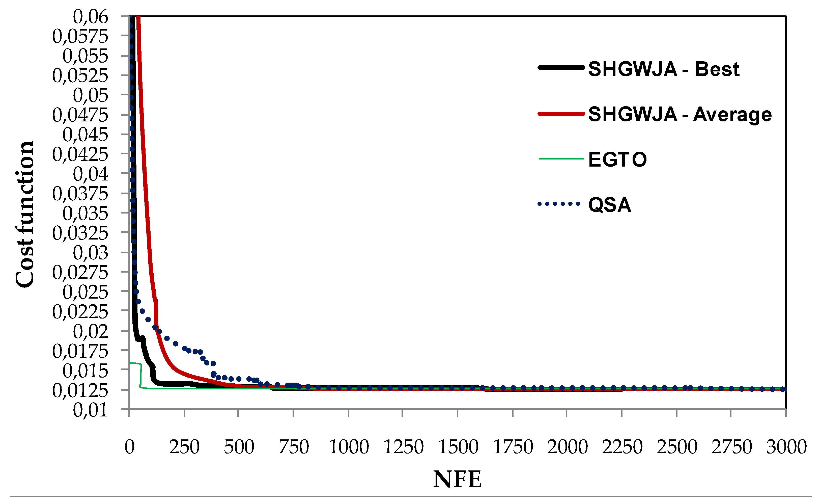
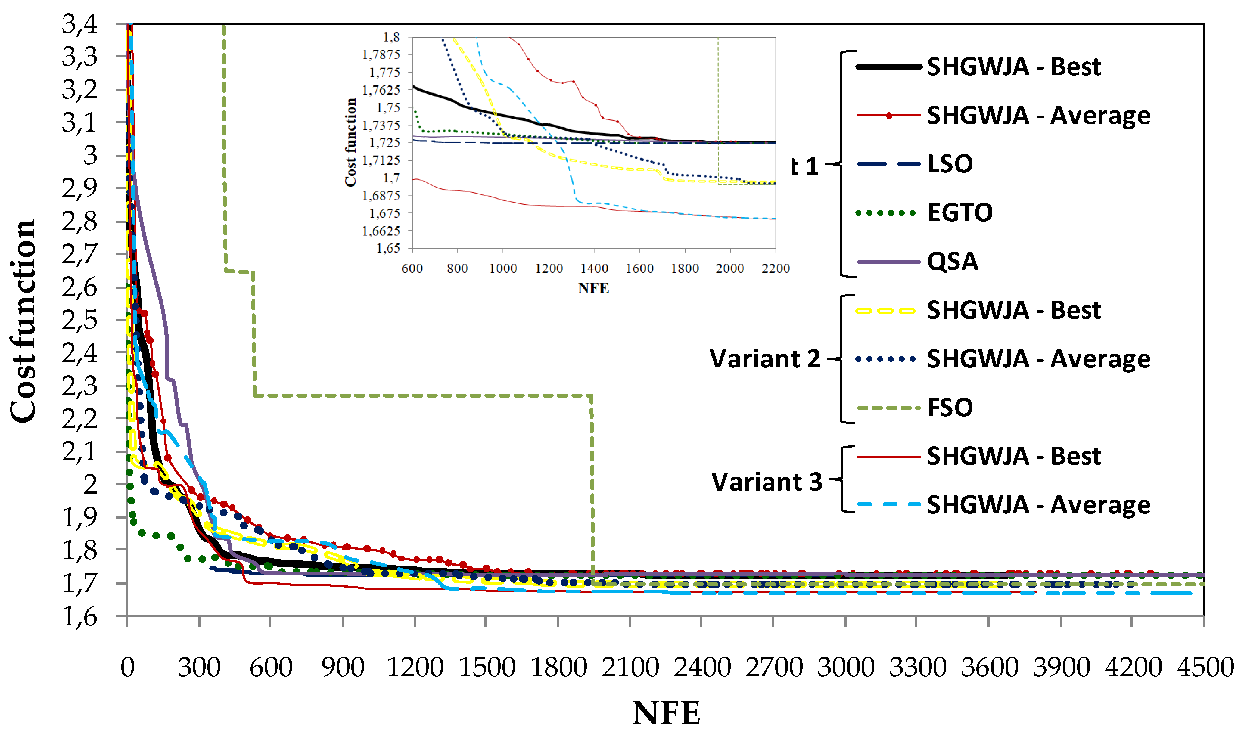
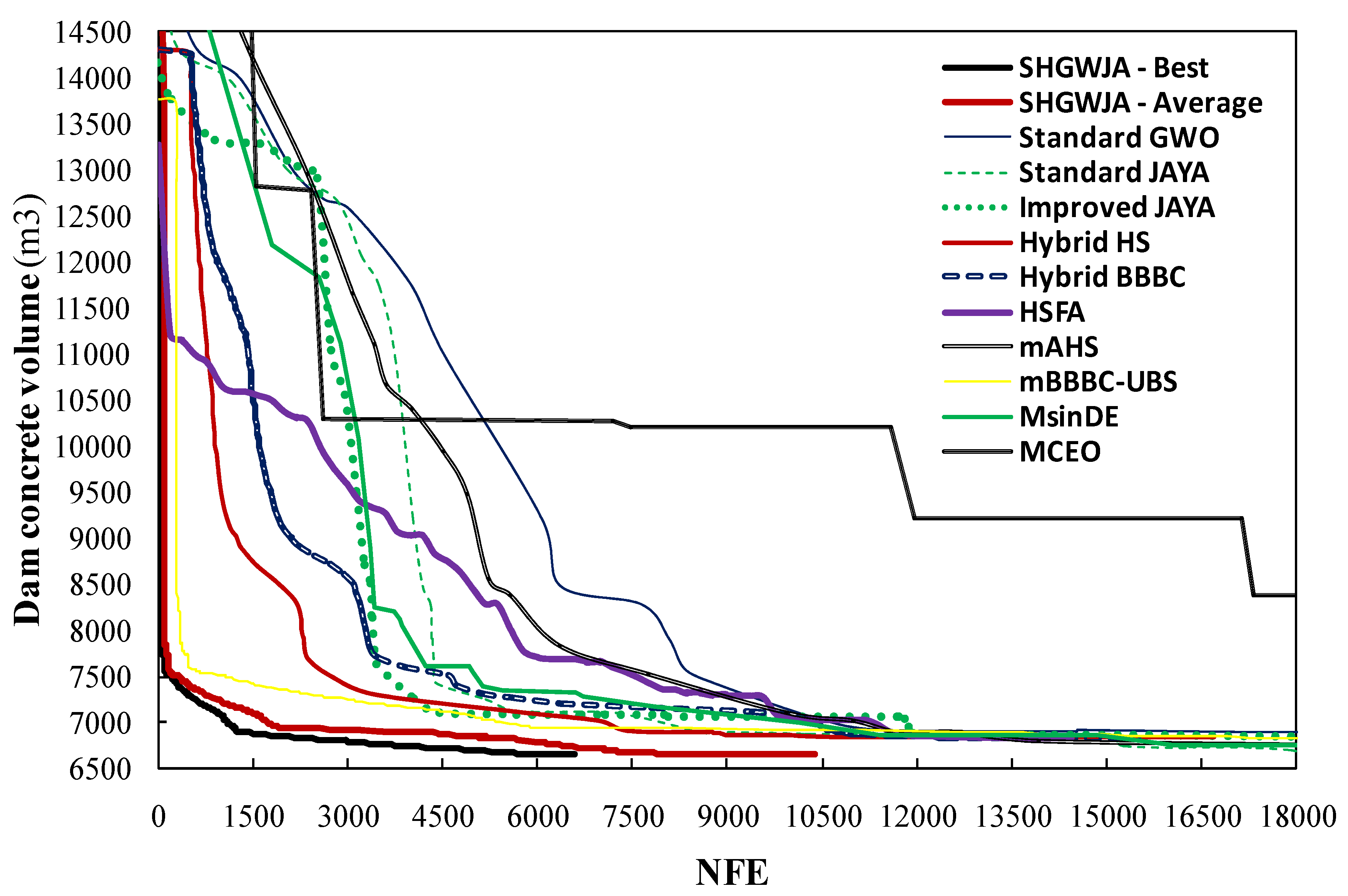
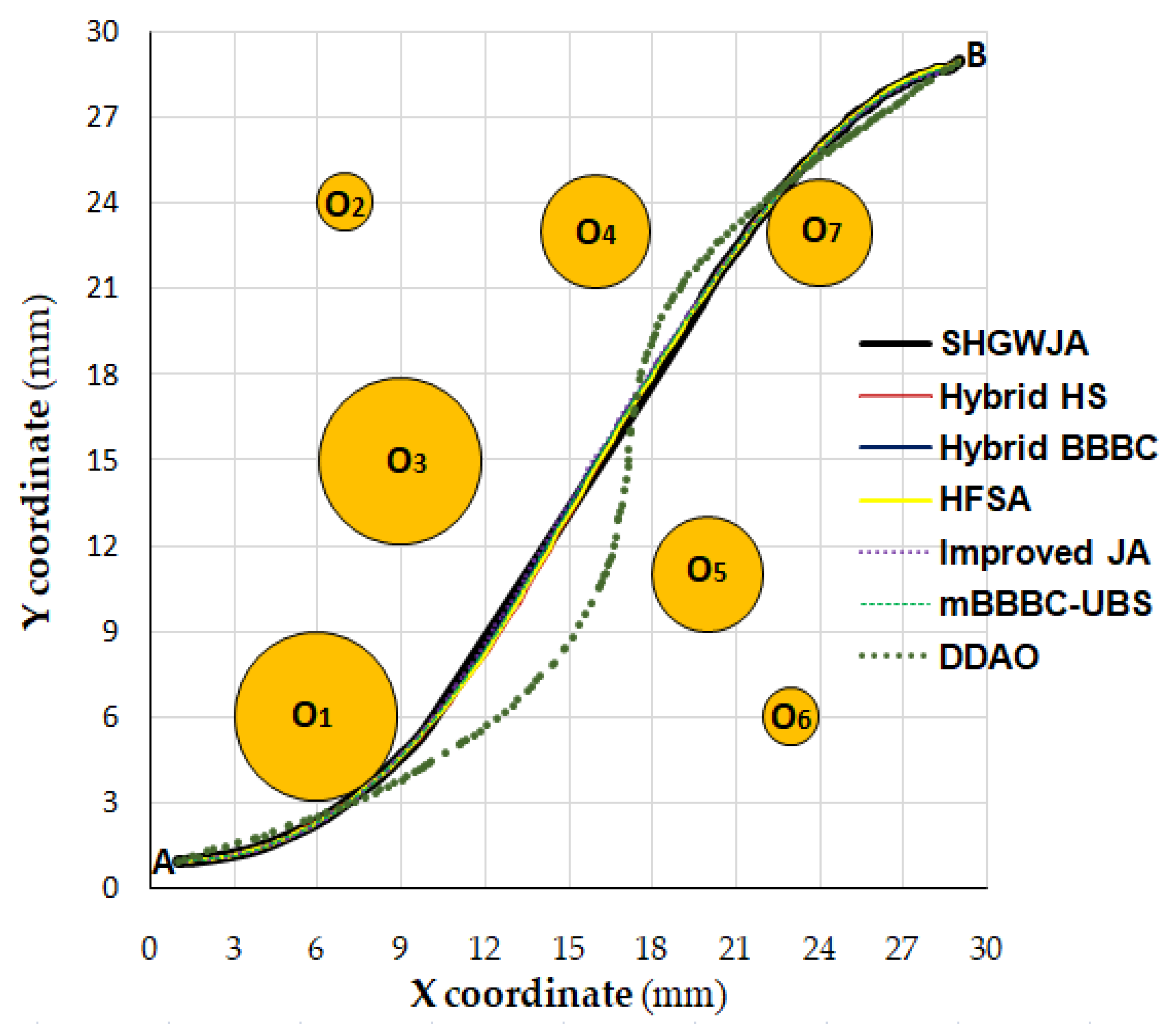