A New Mathematical Approach for Hashimoto’s Thyroiditis in Children

Abstract

Hashimoto’s thyroiditis (HT) is a prevalent autoimmune disorder marked by chronic inflammation of the thyroid gland, predominantly affecting children and adolescents. In a previous study, we developed a “maximal” mathematical model of thyroid physiology to simulate the complex interactions within the thyroid gland. The present research introduces an enhanced version of the “maximal” model, integrating the pathophysiological impacts of HT. It specifically models the adverse effects of thyroid peroxidase (TPO) and thyroglobulin (Tg) antibodies (TPOAb and TgAb) on TPO, Tg, sodium iodide symporter (NIS), albeit indirectly, and thyroid volume. Additionally, we present a new “minimal” model offering a streamlined interpretation of thyroid physiology and pathophysiology, designed for faster computational analysis while maintaining essential physiological interactions. Both models were fitted against longitudinal clinical data from patients with HT, assessing the concentrations of Thyroid Stimulating Hormone (TSH), Thyroxine (T4), and thyroid volume over 36 months, in both untreated patients and those receiving levothyroxine (LT4) treatment. The adaptation of the models to data shows that both of them accurately reproduce the available observed clinical outcomes, with the “maximal” model providing more detailed physiological insights but requiring extensive data and longer computation times. In contrast, the “minimal” model, despite exhibiting less realistic TSH oscillations, offers rapid parameter estimation and may be more feasible in clinical settings. These models hold significant potential as tools for detailed study and management of HT, enabling simulations of disease progression and therapeutic responses, thus paving the way for personalized treatment strategies.

1. Introduction

Hashimoto’s thyroiditis (HT) is an autoimmune disease characterized by chronic inflammation of the thyroid gland, which commonly occurs in children and adolescents [1,2,3]. Adults aged between 40 and 65 are also frequently affected, with a significantly higher prevalence of the disease in women (approximately five times more common) [1]. At diagnosis, patients may be asymptomatic or report symptoms such as goiter, fatigue, altered levels of thyroxine (T4) and thyroid-stimulating hormone (TSH) [4]. Additionally, the presence of thyroid peroxidase (TPOAb) and/or thyroglobulin (TgAb) antibodies is necessary to confirm the autoimmune nature of the disease [5]. The clinical course of HT varies significantly among individuals, making it difficult to predict the behavior of the hormones as well as the changes in thyroid volume over time.

Recently, Pompa et al. [6] presented a “maximal” mathematical model of thyroid physiology; in the present work, the proposed model in [6] is improved to incorporate the pathophysiological aspect derived by the presence of Hashimoto’s thyroiditis, highlighting the different time-courses of TSH and of hormone concentrations, as well as the peculiar trend of the thyroid volume. This updated model reproduces the negative effects of thyroid peroxidase (TPO) and thyroglobulin (Tg) antibodies (TPOAb and TgAb) on TPO, Tg, sodium iodide symporter (NIS) (even if indirectly), and on thyroid volume. These altered behaviors, in turn, lead to changes in TSH and hormone concentrations, which are the key parameters monitored during the treatment of the disease. The therapy for HT involves the administration of levothyroxine (LT4) to restore hormone concentrations to normal ranges [7]. Moreover, in this work a new “minimal” model of the thyroid physiology and pathophysiology, including some of the above features, is presented.

The two models, the improved “maximal” and the “minimal” ones, have been fitted on literature data from Dörr et al. [8], where the concentrations of TSH and T4 and the thyroid volume are collected every 6 months, during 36 months of follow-up from in two groups of euthyroid patients with diagnoses of HT: the first group is composed of not treated subjects (Group 1), whereas the second group (Group 2) is formed by subjects treated with LT4 (50 $\mathsf{\mu }$g for individuals with a bodyweight <50 kg, 75 $\mathsf{\mu }$g for patients with bodyweight between 50 and 75 kg, 100 $\mathsf{\mu }$g for subjects with bodyweight between 75 and 100 kg, and 150 $\mathsf{\mu }$g for adolescents with bodyweight >100 kg).

To our knowledge, the only mathematical model of Hashimoto’s thyroiditis was proposed in [9]. The model includes the equations describing the TSH, thyroxine, TPOAb and the functional size of the thyroid gland, with a daily time scale. This aligns with the model’s objective of replicating and predicting the states of a Hashimoto patient (euthyroidism, subclinical hypothyroidism, and clinical hypothyroidism) over a wide period, without taking into account the oscillations or perturbations of the dynamics of the variables in a short period (hourly). With respect to this model, our mathematical formulation is enlarged to consider, in addition to the above variables, T3 and T4 in both free and bounded forms, the hashitoxicosis phenomenon, the whole thyroid volume (given by the functional size and infiltrating lymphocytes) and the T3 and T4 stored in the thyroid tissue. Moreover, the present models enable a more accurate representation of the variables of interest due to their hourly time discretization. Other works [10,11,12,13,14,15,16,17], as well as the DiStefano III thyroid model [18,19,20,21], provide a description of the thyroid function in pathological conditions without any explicit characterization of HT.

2. “Maximal” Model

This section outlines the updated version of the thyroid model presented by the same Authors [6]. The new formulation is composed of 35 equations, of which 25 differentials and 10 algebraic. The proposed representation describes the most important physiological mechanisms, variables and their interactions (T3, T4, Tg, TSH, TRH, iodine Wolff–Chaikoff control mechanism, antibodies effect and thyroid volume) in the main compartments of the thyroid system (bloodstream, extracellular space, thyroid tissues).

The SIMO model [22] is used to represent the gastrointestinal tract for the iodine, LT4 and LT3 administrations. The SIMO sub-model adds further nine equations (six differential and three algebraic) to the model for a total number of 44 equations. All the model parameters are reported in Table S1 in the Supplementary Material. The next sub-sections report the modifications and updates to the original model. For a detailed description of all the model equations and parameters see the Supplementary Material.

2.1. TRH Sub-Model

Equation (5) of the model in Pompa et al. [6], related to the dynamic of the Thyrotropin-releasing hormone (TRH), is modified to take into consideration the effect of $F{T}_4$ when it falls under the inferior limit of the normality range, which occurs, indeed, in pathological conditions as in the HT:

$${\displaystyle \frac{dTR{H}_N^H}{dt}}=-k_{BN}TR{H}_H^N+\left\{\begin{array}{cc}{Q}_{TR{H}_H^N}^{\#}(e^{-{\gamma }_1^{\#}{T}_{3B}^N}+a_{min1}^{\#})e^{{\gamma }_7^{\#}(T_{FT4}-F{T}_4)}\hfill & F{T}_4<T_{FT4}\hfill \\ Q_{TR{H}_H^N}^{\#}(e^{-{\gamma }_1^{\#}{T}_{3B}^N}+a_{min1}^{\#})({\displaystyle \frac{a_{max1}}{m+{(F{T}_4-T_{FT4})}^{{\gamma }_2^{\#}}}}+a_{min2}^{\#})\hfill & F{T}_4\ge T_{FT4}\hfill \end{array}\right.$$

(1)

$$TR{H}_H^N\left(0\right)=TR{H}_{H0}^N$$

where:

• $TR{H}_H^N$ is a normalized variable representing the TRH in the hypothalamus;
• $e^{{\gamma }_7^{\#}(T_{FT4}-F{T}_4)}$ is the new term of the equation that represents the relationship between $TR{H}_N^H$ and $F{T}_4$: when the $F{T}_4$ is below the normality threshold, the production of $TR{H}_N^H$ increases causing the consequent increase in TSH;
• $T_{FT4}$ represents the threshold to which TSH changes its dynamic and it is set to 1.35 ng/dL, that is to the average value of the normal FT4 range, which is between 0.8 and 1.9 ng/dL (or 10.3 and 24.5 pmol/L) [23,24].

The missing equations of the TRH dynamics, TSH and biological oscillator are reported in the Supplementary Materials (Equations (S10)–(S18)).

2.2. Wolff–Chaikoff Sub-Model

When a high concentration of iodine is ingested (as occurs through the intake of drugs or food), the thyroid attempts to protect itself by blocking specific functions. Generally, the sodium iodine symporter transports iodine into the thyroid. However, when the internal iodine concentration exceeds ${10}^{-3}$ molar (in a normal thyroid), thyroglobulin organification ceases to function, thereby blocking the T3 and T4 hormone production [25,26]. At this point, the NIS ceases to transport iodine into the thyroid, allowing excess iodine to flow back into the bloodstream. This process is called the Wolff–Chaikoff effect. This control system induces a temporary state of hypothyroidism, which lasts for the time it takes for iodine levels in the thyroid to return to normal concentration values (usually in about one week). When the iodine concentration drops below ${10}^{-3}$ molar, the normal thyroid functions resume.

The above control process, which in this dissertation is named $C_{wc}$, is described as follows: starting from $C_{wc}\left(0\right)=0$ , the Wolff–Chaikoff effect can be formalized by means of the following hybrid dynamics [27]

$$\left\{\begin{array}{cc}{C}_{wc}\leftarrow 0\hfill & \mathrm{if}{C}_{wc}=1\mathrm{and}{I}_T=I_{wmin}{V}_T^N\hfill \\ C_{wc}\leftarrow 1\hfill & \mathrm{if}{C}_{wc}=0\mathrm{and}{I}_T=I_{wmax}{V}_T^N\hfill \\ {\displaystyle \frac{d{C}_{wc}}{dt}}=0\hfill & \mathrm{otherwise}\hfill \end{array}\right.$$

(2)

where the symbol ← denotes the instantaneous reset of the state variable.

The $C_{wc}$ function is 0 when the iodine is below the maximum threshold ($I_{wmax}{V}_T^N$) and becomes 1 when it exceeds that threshold. Furthermore, once $C_{wc}$ becomes 1, it maintains this value until the iodine concentration returns to the minimum threshold ($I_{wmin}{V}_T^N$). When $C_{wc}$ is equal to 1, as described in the next sub-section, the equations related to the extracellular iodine and to the iodine inside the thyroid change their dynamics in relation to iodine transportation (from the internal to extracellular space). Additionally, the TPO variable is set to 0, in order to represent the cessation of the T3 and T4 production.

2.3. Iodine Sub-Model

The iodine sub-model is similar to the formalization adopted in the original work [6], except for the introduction of the Wolff–Chaikoff control (Equations (4) and (5)) as well as for the consideration of the effect of the antibodies and thyroid volume on NIS and TPO efficacy (Equations (6) and (7)):

$$\begin{array}{cc}\hfill & {\displaystyle \frac{d{I}_B}{dt}}={\displaystyle \frac{R_{aI}}{V_B^L}}-k_{EBI}{I}_B-k_{kid}{I}_B+10{\displaystyle \frac{1}{6}}[{\displaystyle \frac{v_{T4}{T}_{4B}}{k_{MT4}+T_{4B}}}{(1-{\displaystyle \frac{T_{3B}}{T_{T3}}})}^{{\gamma }_6^{\#}}+{\displaystyle \frac{v_{T4dly}{T}_{4dly}}{k_{MT4dly}+T_{4dly}}}]+\hfill \\ \hfill & +{\displaystyle \frac{k_{BEI}{I}_E}{V_B^L}}+10[0.65k_{xT4}{T}_{4B}+0.59(k_{xT3}{T}_{3B}+{\displaystyle \frac{v_{T3}{T}_{3B}}{k_{MT3}+T_{3B}}})],I_B\left(0\right)=I_{B0}\hfill \end{array}$$

(3)

$${\displaystyle \frac{d{I}_E}{dt}}=\left\{\begin{array}{cc}{k}_{EBI}{I}_B{V}_B^L-NIS{I}_E-k_{BEI}{I}_E\hfill & C_{wc}=0\hfill \\ k_{wc}{I}_T-k_{BEI}{I}_E+k_{EBI}{I}_B{V}_B^L\hfill & C_{wc}=1\hfill \end{array}\right.,I_E\left(0\right)=I_{E0}$$

(4)

$${\displaystyle \frac{d{I}_T}{dt}}=\left\{\begin{array}{cc}NIS{I}_E-{\displaystyle \frac{v_{IT1}TPO{I}_T}{k_{IM}+I_T}}\hfill & C_{wc}=0\hfill \\ -k_{wc}{I}_T\hfill & C_{wc}=1\hfill \end{array}\right.,I_T\left(0\right)=I_{T0}$$

(5)

$$NIS=k_{NIS}{V}_f{e}^{-L_{dly}}({\displaystyle \frac{k_{NIS1}^{\#}TS{H}^{N{\gamma }_4^{\#}}}{k_{NIS2}^{\#{\gamma }_4^{\#}}+TS{H}^{N{\gamma }_4^{\#}}}})$$

(6)

$$TPO=\left\{\begin{array}{cc}{k}_{TPO}^{\#}{V}_f{e}^{-L_{dly}}({\displaystyle \frac{k_{TPO1}^{\#}TS{H}^{N{\gamma }_3^{\#}}}{k_{TPO2}^{\#}+TS{H}^{N{\gamma }_3^{\#}}}})\hfill & I_T\le 0.95I_{wmax}\hfill \\ 0\hfill & I_T>0.95I_{wmax}{V}_T^N\hfill \end{array}\right.$$

(7)

where:

• the variables $I_B$, $I_E$, $I_T$ are the iodine in the blood, extracellular and thyroid compartments, respectively;
• $TPO$ represents the effect of the thyroid peroxidase;
• $NIS$ represents the effect of the sodium iodide symporter;

The antibody effect $L_{dly}$ has a direct impact on both $TPO$ and $NIS$: TPO functionality decreases when thyroid peroxidase antibodies (TPOAbs) attack the thyroid with the aim of interrupting the TPO functionalities or of destroying the enzymes; similarly, NIS efficacy also decreases due to the presence of cytokines induced by the thyroid inflammation [28].

2.4. Antibodies Sub-Model

Hashimoto’s thyroiditis causes the organism to produce thyroid TPOAbs and TgAbs, which attack and destroy the thyroid tissue. This phenomenon progressively reduces the thyroid’s ability to produce hormones until it eventually becomes completely inefficient.

The precise mechanisms leading the organism to produce TPOAb and TgAb remain unknown, making it impossible to develop a mathematical representation of the phenomenon, it is possible to model the effects of these antibodies on the thyroid function once HT manifests. The effect of antibodies and its trend over time is represented by the following forcing function:

$$E_{ant}=1-e^{-k_{ant}(t-\tau )},t\ge \tau$$

(8)

where:

• $E_{ant}$ represents the antibodies effect: it starts from 0, increases with a speed equal to $k_{ant}$ until reaching 1;
• $\tau$ is the time at which the antibody effect manifests.

The $E_{ant}$ function increases the volume of the lymphocyte compartment (which is part of the total thyroid volume). The lymphocyte volume, in its turn, affects the $TPO$ and $NIS$ variables.

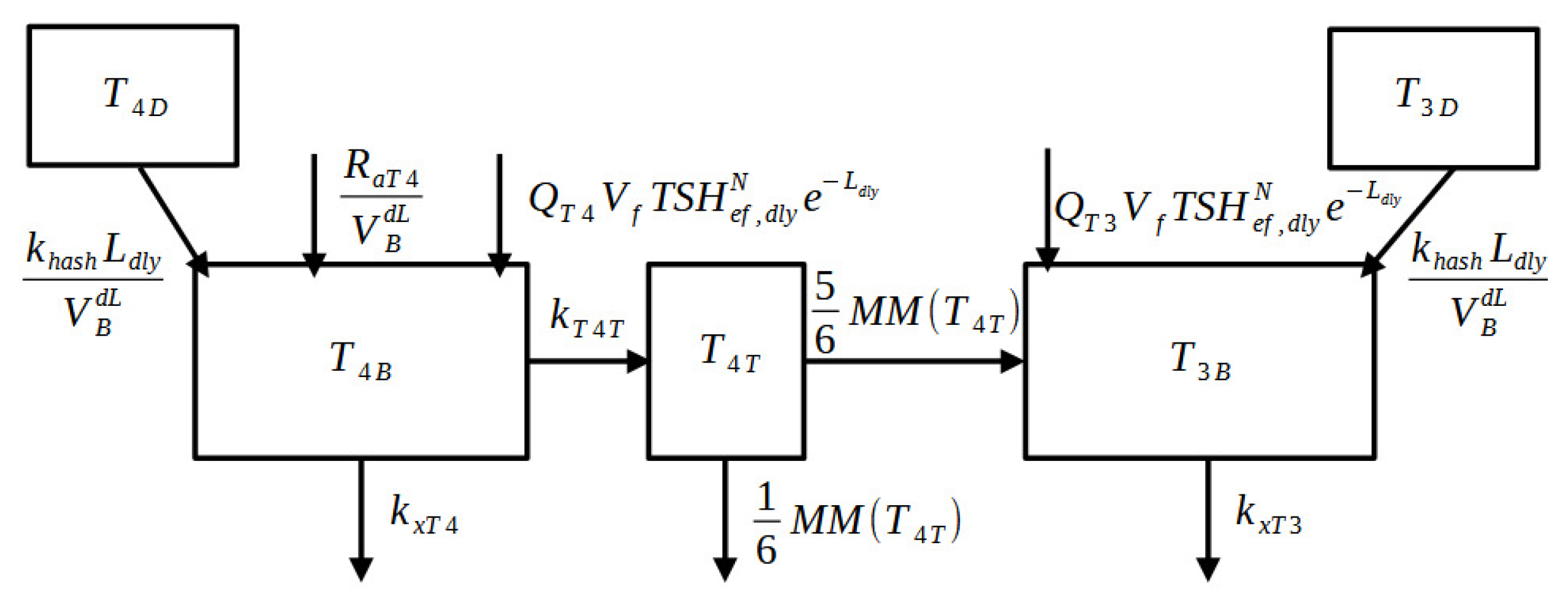
2.5. Thyroid Volume Sub-Model

An important feature introduced in this new version of the model is the representation of the thyroid volume time course. The volume depends directly on the TSH concentration, as thyroid cells proliferate more in the presence of higher TSH levels. Furthermore, all the thyroid physiological functions are strictly related to the volume [4].

In the initial phase of the HT disease, the thyroid volume typically increases due to lymphocyte infiltration within the gland, causing inflammation. Afterwards, the total thyroid volume starts to decrease as TPOAbs and TgAbs (the infiltrated lymphocytes) attack and destroy the thyroid tissue until the gland completely disappears. This process can take many years, usually exceeding 10 years, and varies from individual to individual. A block diagram of the thyroid volume sub-model is shown in Figure 1.

The equations are reported below:

$${\displaystyle \frac{dL}{dt}}=k_{LV}{E}_{ant}{V}_f-k_{xL}L,L\left(0\right)=L_0$$

(9)

$${\displaystyle \frac{d{L}_{dly}}{dt}}=k_{dlyL}(L-L_{dly}),L_{dly}\left(0\right)=L_0$$

(10)

$${\displaystyle \frac{d{V}_f}{dt}}=k_{TSHx}TS{H}_{ef,dly}^N{V}_f-k_{xVf}{V}_f-k_{xVfL}{L}_{dly}{V}_f,V_f\left(0\right)=V_{f0}$$

(11)

$$V_T^N=L+V_f$$

(12)

where:

• L is the lymphocyte volume compartment;
• $L_{dly}$ is the delayed version of L, simulating the delayed effect of the lymphocytes on the thyroid functionalities;
• $V_f$ is the functional thyroid volume compartment;
• $V_T^N$ is the total thyroid volume.

2.6. Hormone Sub-Model

During the early stage of the HT disease, the destruction of the gland can lead to an increase in T3 and T4 hormone concentrations. This occurs as the hormones stored within the thyroid are released into the bloodstream. This phenomenon, known as “hashitoxicosis”, results in a transient hyperthyroid state [29,30]. The modified version of the T3 and T4 equations are reported below:

$${\displaystyle \frac{d{T}_{3D}}{dt}}=-k_{hash}{T}_{3D}{L}_{dly}+k_{DPT3}{T}_{3P}-k_{PDT3}{T}_{3D},T_{3D}\left(0\right)=T_{3D0}$$

(13)

$${\displaystyle \frac{d{T}_{3P}}{dt}}={\displaystyle \frac{v_{IT2}TPO{I}_T{\beta }_{T3}^{\#}\frac{P_{T3}}{3}}{k_{IM}+I_T}}-k_{EPT3}{T}_{3P}TS{H}_{ef,dly}^N-k_{DPT3}{T}_{3P}+k_{PDT3}{T}_{3D},T_{3P}\left(0\right)=T_{3P0}$$

(14)

$${\displaystyle \frac{d{T}_{3E}}{dt}}=k_{EPT3}{T}_{3P}TS{H}_{ef,dly}^N-k_{BET3}{T}_{3E},T_{3E}\left(0\right)=T_{3E0}$$

(15)

$$\begin{array}{cc}\hfill & {\displaystyle \frac{d{T}_{3B}}{dt}}={\displaystyle \frac{k_{BET3}{T}_{3E}}{V_B^{dL}}}-k_{xT3}{T}_{3B}+{\displaystyle \frac{k_{hash}{T}_{3D}{L}_{dly}}{V_B^{dL}}}+{\displaystyle \frac{5}{6}}[{\displaystyle \frac{v_{T4}{T}_{4B}}{k_{MT4}+T_{4B}}}{(1-{\displaystyle \frac{T_{3B}}{T_{T3}}})}^{{\gamma }_6^{\#}}+\hfill \\ \hfill & +{\displaystyle \frac{v_{T4dly}{T}_{4dly}}{k_{MT4dly}+T_{4dly}}}]-{\displaystyle \frac{v_{T3}{T}_{3B}}{k_{MT3}+T_{3B}}}+{\displaystyle \frac{R_{aT3}}{V_B^{dL}}},T_{3B}\left(0\right)=T_{3B0}\hfill \end{array}$$

(16)

$${\displaystyle \frac{d{T}_{4D}}{dt}}=-k_{hash}{T}_{4D}{L}_{dly}+k_{DPT4}{T}_{4P}-k_{PDT4}{T}_{4D},T_{4D}\left(0\right)=T_{4D0}$$

(17)

$${\displaystyle \frac{d{T}_{4P}}{dt}}={\displaystyle \frac{v_{IT2}TPO{I}_T{\beta }_{T4}^{\#}\frac{P_{T4}}{4}}{k_{IM}+I_T}}-k_{EPT4}{T}_{4P}TS{H}_{ef,dly}^N-k_{DPT4}{T}_{4P}+k_{PDT4}{T}_{4D},T_{4P}\left(0\right)=T_{4P0}$$

(18)

$${\displaystyle \frac{d{T}_{4E}}{dt}}=k_{EPT4}{T}_{4P}TS{H}_{ef,dly}^N-k_{BET4}{T}_{4E},T_{4E}\left(0\right)=T_{4E0}$$

(19)

$$\begin{array}{cc}\hfill & {\displaystyle \frac{d{T}_{4B}}{dt}}={\displaystyle \frac{k_{BET4}{T}_{4E}}{V_B^{dL}}}+{\displaystyle \frac{k_{hash}{T}_{4D}{L}_{dly}}{V_B^{dL}}}-k_{xT4}{T}_{4B}-{\displaystyle \frac{v_{T4}{T}_{4B}}{k_{MT4}+T_{4B}}}{(1-{\displaystyle \frac{T_{3B}}{T_{T3}}})}^{{\gamma }_6^{\#}}-k_{dlyB}{T}_{4B}+\hfill \\ \hfill & +{\displaystyle \frac{R_{aT4}}{V_B^{dL}}},T_{4B}\left(0\right)=T_{4B0}\hfill \end{array}$$

(20)

where:

• $T_{3D}$ and $T_{4D}$ represent the quantity of T3 and T4 in the depot compartment;
• $T_{3P}$ and $T_{4P}$ represent the quantity of T3 and T4 in the thyroid compartment;
• $T_{3E}$ and $T_{4E}$ represent the quantity of T3 and T4 in the extra cellular compartment;
• $T_{3B}$ and $T_{4B}$ represent the T3 and T4 concentrations in the blood compartment;
• $k_{hash}{T}_{3D}{L}_{dly}$ and $k_{hash}{T}_{4D}{L}_{dly}$, in Equations (13) and (17), respectively, represent the effect of the hashitoxicosis on the release of stocked T3 and T4. In the two equations, the same hashitoxicosis rate ($k_{hash}$) for the two hormones is assumed, as the thyroid cells destroyed by antibodies contain both T4 and T3. Different released quantities depend on the different $T_{3D}$ and $T_{4D}$ values at time t.

The description of the T3 and T4 dynamics are reported in the Supplementary Materials (Equations (S19)–(S23)).

2.7. Tg Sub-Model

Thyroglobulin antibodies specifically target and destroy thyroglobulin in the blood, leading to a reduction in its concentration. This effect is incorporated into the Tg blood concentration equations using the forcing function, $E_{ant}$. These changes are reported below:

$${\displaystyle \frac{d{T}_{gE}^N}{dt}}=Q_{T4Tg}{T}_{4E}^N+E_{ant}{k}_{des}{V}_T^N-k_{BETg}{T}_{gE}^N,T_{gE}^N\left(0\right)=T_{gE0}^N$$

(21)

$${\displaystyle \frac{d{T}_{gB}}{dt}}=k_{BETg}{T}_{gE}^N{Q}_{Tg}-k_{xTg}{T}_{gB}(1+E_{ant}),T_{gB}\left(0\right)=T_{gB0}$$

(22)

where the variables $T_{gE}^N$ and $T_{gB}$ are the Tg in the extracellular and ($T_4$ and $T_3$) blood compartments, respectively. Note that, as for the previous version of the model, it is not possible to validate the Tg sub-model since no data related to Tg blood concentrations are available from literature.

3. “Minimal” Model

The thyroid “minimal” model was derived as a simplification of the updated version of the “maximal” model described above and in the Supplementary Material, and is composed of only 16 equations (replacing the original 35 equations), eight differential and eight algebraic. Some equations are in common with the two versions (from Equations (8) to (12) and both need to be accompanied by the SIMO sub-model for the representation of per os drug administration). All the model parameters are reported in Table S2 of the Supplementary Material. The next two subsections report the only equations which differ in the two formulations. Figure 1 and Figure 2 show the block diagram of the new “minimal” model.

3.1. TSH Sub-Model

The TSH blood concentration is modeled using a simple sinusoidal function to reduce the number of equations required to represent the hypothalamus–pituitary–thyroid axis. The equations regarding the TSH sub-model are reported below:

$$\begin{array}{cc}\hfill & {\displaystyle \frac{dTSH}{dt}}=-k_{h}TSH+[k_{TSHbas}+k_{T3T4}sin({\displaystyle \frac{2\pi }{24}}t-\phi )]e^{-{\lambda }_1^{\#}F{T}_3\ast F{T}_4},\hfill \\ \hfill & TSH\left(0\right)=TS{H}_0\hfill \end{array}$$

(23)

$$TS{H}^N={\displaystyle \frac{TSH}{\overline{TSH}}},$$

(24)

$$TS{H}_{ef}^N={\displaystyle \frac{k_{TSH1}TS{H}^{N{\lambda }_2^{\#}}}{k_{TSH2}+TS{H}^{N{\lambda }_2^{\#}}}}+k_{TSH3}$$

(25)

$${\displaystyle \frac{dTS{H}_{ef,dly}^N}{dt}}=k_{TSHdly}(TS{H}_{ef}^N-TS{H}_{ef,dly}^N),TS{H}_{ef,dly}^N\left(0\right)=TS{H}_0^N$$

(26)

where:

• $TSH$ is the variable representing the Thyroid-stimulating hormone;
• $TS{H}_{ef}^N$ and $TS{H}_{ef,dly}^N$ are the direct and delayed effects of TSH on the T3 and T4 production.

The feedback control between $TSH$ and the hormones is represented by the exponential term $e^{-{\lambda }_1^{\#}F{T}_{3}F{T}_4}$. Equation (23) is derived from the DiStefano III formulation [31] with some changes in the exponential term in order to directly represent the disjunct effect of FT4 and FT3 on TSH.

3.2. T3 and T4 Hormone Sub-Model

The description of the hormone time courses has been simplified by considering only the concentrations of T3 and T4 in the blood ($T_{3B}$ and $T_{4B}$) as well as the concentration of T4 in the tissue ($T_{4T}$). In this reduced formulation the production of the hormones is represented by a constant parameter Q multiplied by $TS{H}_{ef,dly}^N$ and $V_f$ to represent the dependence of the production on both TSH and the functional thyroid volume. In this version of the model no per os T3 administration is foreseen. The sub-model equations are reported below:

$$T_{4D}=T_{4D0}{e}^{-k_{hash}{L}_{dly}t}$$

(27)

$$\begin{array}{cc}\hfill & {\displaystyle \frac{d{T}_{4B}}{dt}}=Q_{T4}TS{H}_{ef,dly}^N{V}_f{e}^{-L_{dly}}-k_{xT4}{T}_{4B}-k_{T4T}{T}_{4B}+{\displaystyle \frac{R_{aT4}}{V_B^{dL}}}+{\displaystyle \frac{k_{hash}{L}_{dly}{T}_{4D}}{V_B^{dL}}},\hfill \\ \hfill & T_{4B}\left(0\right)=T_{4B0}\hfill \end{array}$$

(28)

$${\displaystyle \frac{d{T}_{4T}}{dt}}=k_{T4T}{T}_{4B}-{\displaystyle \frac{v_d{T}_{4T}}{k_{MTd}+T_{4T}}},T_{4T}\left(0\right)=T_{4T0}$$

(29)

$$F{T}_4=fra{c}_{T4}^{\#}{T}_{4B}$$

(30)

$$T_{3D}=T_{3D0}{e}^{-k_{hash}{L}_{dly}t}$$

(31)

$$\begin{array}{cc}\hfill & {\displaystyle \frac{d{T}_{3B}}{dt}}=Q_{T3}TS{H}_{ef,dly}^N{V}_f{e}^{-L_{dly}}-k_{xT3}{T}_{3B}+{\displaystyle \frac{5}{6}}{\displaystyle \frac{v_d{T}_{4T}}{k_{Md}+T_{4T}}}+{\displaystyle \frac{k_{hash}{L}_{dly}{T}_{3D}}{V_B^{dL}}},\hfill \\ \hfill & T_{3B}\left(0\right)=T_{3B0}\hfill \end{array}$$

(32)

$$F{T}_3=fra{c}_{T3}^{\#}{T}_{3B}$$

(33)

where:

• $T_{3D}$ and $T_{4D}$ represent the T3 and T4 quantities in the depot compartment;
• $T_{4T}$ is the T4 concentration in the tissue compartment;
• $T_{3B}$ and $T_{4B}$ represent the T3 and T4 concentrations in the blood compartment;
• the $k_{hash}{T}_{3D}{L}_{dly}$ and $k_{hash}{T}_{4D}{L}_{dly}$ terms represent the hashitoxicosis.

4. Gut Sub-Model

The SIMO model [22] is utilized as a gastrointestinal sub-model to describe iodine (represented by I) intake and the fate of administered LT4 and LT3 (represented by $T4$ and $T3$, respectively). This sub-model incorporates nine additional equations into the maximal model (time-course of Iodine, LT4 and LT3) and three (time-course of LT4) into the minimal model. The letter S denotes the stomach compartment, L represents the ileum, and $R_a$ signifies the rate of appearance of a substance.

4.1. Iodine

$${\displaystyle \frac{d{S}_I}{dt}}=-k_{lsI}{S}_I+D_I\delta \left(t\right),S_I\left(0\right)=S_{I0}$$

(34)

$${\displaystyle \frac{d{L}_I}{dt}}=k_{lsI}{S}_I-k_{blI}{L}_I,L_I\left(0\right)=L_{I0}$$

(35)

$$R_{aI}=k_{blI}{L}_I{f}_I,R_{aI}\left(0\right)=R_{aI0}$$

(36)

4.2. LT4

$${\displaystyle \frac{d{S}_{T4}}{dt}}=-k_{lsT4}{S}_{T4}+D_{T4}\delta \left(t\right),S_{T4}\left(0\right)=S_{T40}$$

(37)

$${\displaystyle \frac{d{L}_{T4}}{dt}}=k_{lsT4}{S}_{T4}-k_{blT4}{L}_{T4},L_{T4}\left(0\right)=L_{T40}$$

(38)

$$R_{aT4}=k_{blT4}{L}_{T4}{f}_{T4},R_{aT4}\left(0\right)=R_{aT40}$$

(39)

4.3. LT3

$${\displaystyle \frac{d{S}_{T3}}{dt}}=-k_{lsT3}{S}_{T3}+D_{T3}\delta \left(t\right),S_{T3}\left(0\right)=S_{T30}$$

(40)

$${\displaystyle \frac{d{L}_{T3}}{dt}}=k_{lsT3}{S}_{T3}-k_{blT3}{L}_{T3},L_{T3}\left(0\right)=L_{T30}$$

(41)

$$R_{aT3}=k_{blT4}{L}_{T3}{f}_{T3},R_{aT3}\left(0\right)=R_{aT30}$$

(42)

5. Model Parameter Estimation

The “minimal” model was fitted on data from [8] where an experiment was carried out to determine the efficacy of per os LT4 administration in an adolescent recently suffering from Hashimoto thyroiditis. Patients were randomly allocated to two groups: 25 individuals received LT4 at a mean daily dose of 1.6 $\mathsf{\mu }$g/kg (50 $\mathsf{\mu }$g for individuals with a bodyweight <50 kg, 75 $\mathsf{\mu }$g for patients with a bodyweight between 50 and 75 kg, 100 $\mathsf{\mu }$g for subjects with a bodyweight between 75 and 100 kg, and 150 $\mathsf{\mu }$g for adolescents with a bodyweight >100 kg), and 34 individuals were not treated. The main outcomes were the thyroid gland volume (determined by ultrasound), the serum levels of TSH, the free T4 concentrations, the concentrations of the antibodies against thyroid peroxidase and of the thyroglobulin. All these parameters were assessed every 6 months for a total of 36-month follow-up. The children in both groups were assumed to weigh 45 kg and for Group 2 the LT4 dose was administered according to the original experimental protocol (50 $\mathsf{\mu }$g).

The model was adapted to data by means of a Weighted Least-Squares approach where the differences between observations and predictions have been weighted with the inverse of the squared expectations, hypothesizing an error variance proportional to the coefficient of variation of the observations. The algorithm used for the minimization of the loss function was the Nelder–Mead scheme. The numerical integration method employed to solve the Ordinary Differential Equations (ODEs) was the fourth order Runge–Kutta method (RK4). The implementation was carried out with Matlab^®. The parameters included in the estimation procedure were all the parameters appearing in the equations of the new Thyroid Volume sub-model, plus the parameters $\overline{T4D}$ and $\overline{T3D}$, which are considered important in determining the dynamics of HT.

The “minimal” model resulted in a significantly shorter simulation and parameter estimation time when compared with the “maximal” model.

The parameter estimation process for the “maximal” model followed a two-step approach: a first estimated parameter vector (composed of eighteen parameters) was obtained by adapting the “minimal” model to observed data; the estimates obtained were subsequently used as a starting point for the calibration of the “maximal” model parameters, which were then fine-tuned. Additionally, to prevent the TSH oscillation from influencing the value of the loss function, the mean of the upper and lower envelope curves (expressing the magnitude of the TSH signal) was employed as a representation of the TSH time course.

6. Sensitivity Analysis

A sensitivity analysis of the original maximal model was presented in [6]. Given the model’s complexity (due to its numerous parameters), which increased in the present updated formulation including the HT representation, a sensitivity analysis was conducted by varying only those parameters entering the additional Thyroid Volume sub-model of the minimal version. The sensitivity analysis was performed by varying 30% of the parameter values obtained by the estimation procedure on the treated subjects’ observations. The parameters of interest, and that were allowed to vary, were eight out of thirteen, that is the subset of parameters involved in the description of the HT pathophysiological mechanisms. For each of the eight parameters, 100 simulations with a one-year time window were run. The predictions of TSH, FT4, and Volume over time obtained with the baseline parameter values are compared to the 90% envelopes of forecasts from the sensitivity analysis, alongside the experimental data. To assess the combined impact of parameter variations, an additional series of 100 simulations were performed, simultaneously varying all eight parameters. For the TSH and FT4, the figures show a zoom of the last 200 h for better visualization of the results.

7. Results

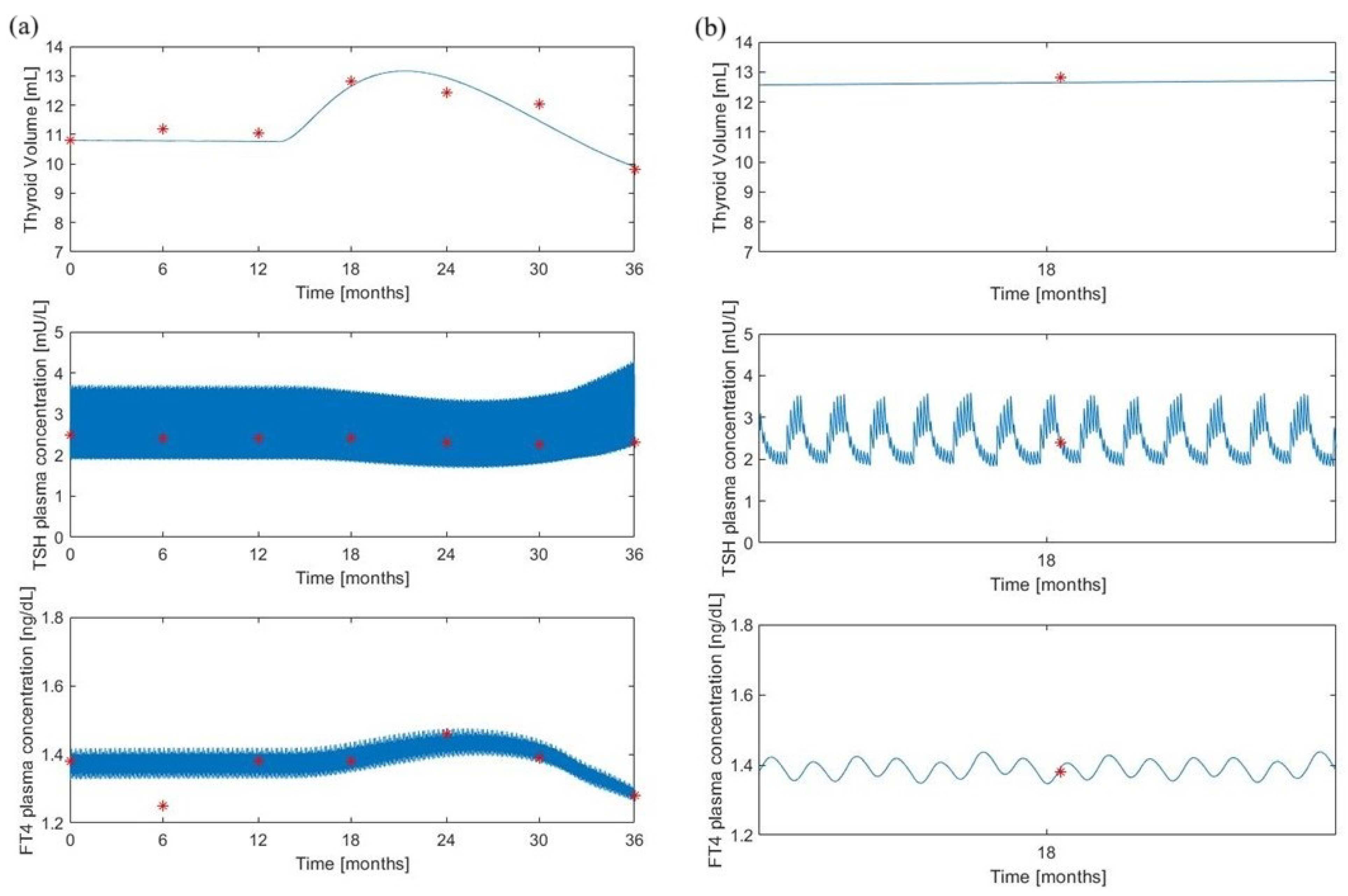
This section shows the performance of the two model formulations, the “maximal” model (updated version, as described in the “Maximal” Model section) and the “minimal” model.

Figure 3 shows the model predictions of the volume, TSH and FT4 variables, obtained from the “maximal” model, over a 36-month simulation period, along with the observed data points (red circles) from the untreated subjects (Group 1) of [8]. Panel (b) is an enlargement at month 18 of the time courses shown in panel (a).

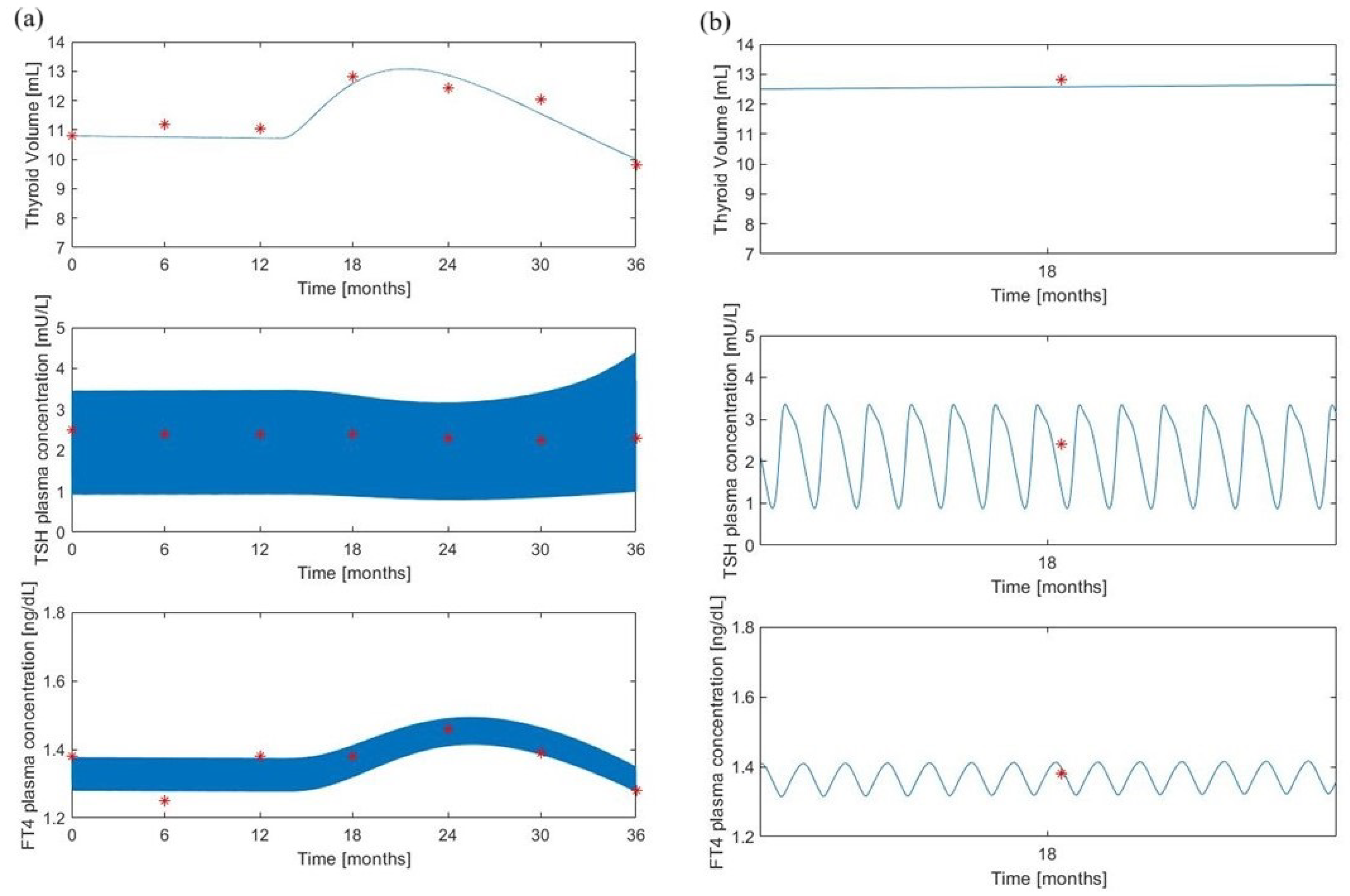
Figure 4 reports the same experimental data of Figure 3 along with the corresponding predictions obtained with the “minimal” model.

Despite a similar qualitative behavior, the “minimal” model produces larger oscillations of the TSH which appear to be less realistic than those obtained with the “maximal” model. The “maximal” model, in fact, demonstrates a more detailed pattern, deviating from a simple sinusoidal waveform. This more realistic trend is attributed to the biological oscillator equations presented in the Supplementary Materials (Equations (S10)–(S12)) and previously discussed in Pompa et al [6]. On the contrary, the volume predictions appear to be superimposed while the FT4 “minimal” model predictions lie in a slightly larger interval.

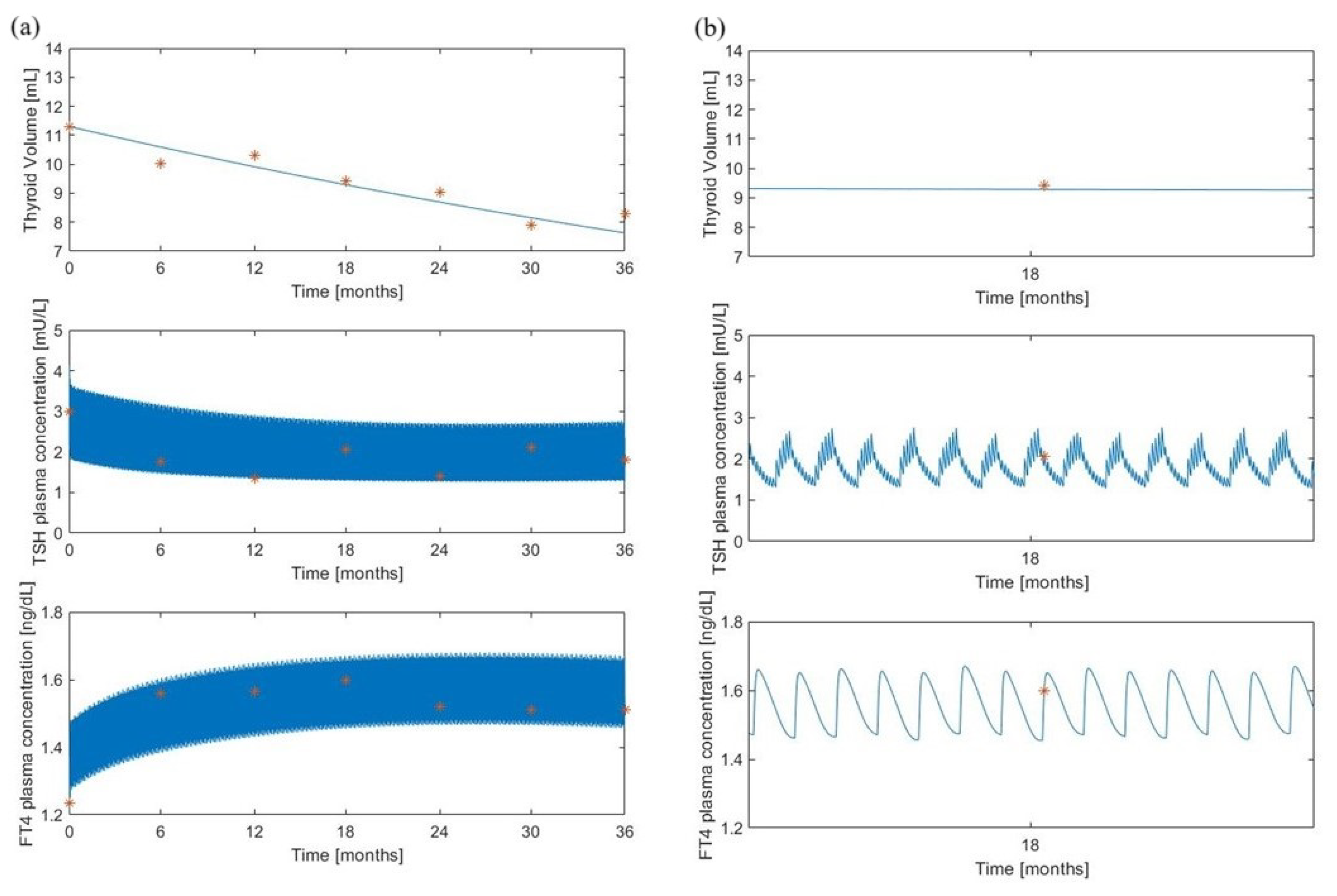
Figure 5 and Figure 6 show the corresponding variables (observed and predicted) for the treated subjects (Group 2) of [8].

Here, it was assumed a daily administration of 50 $\mathsf{\mu }$g of LT4 which represents the administered dosage for a subject of 45 kg, according to the original protocol adopted in [8]. Refer to the “Method” section of [8] for details on the experimental procedure. Also in this situation, the qualitative behavior of the “minimal” model resembles the “maximal” model pattern and the volume predictions are in line with the observations.

All the parameter values obtained from the optimization or calibration procedures are reported in

Table 1. Parameter values from the optimization process (for the “minimal” model) and from the calibration procedure (for the “maximal” model) for the untreated subjects (Group 1) and for treated subjects (Group 2).

	Group 1		Group 2
	“Maximal” Model	“Minimal” Model	“Maximal” Model	“Minimal” Model
$\tau$ [h]	9774.62	9774.62	−3524.77	−3524.77
$k_{ant}$ [1/h]	3.946 × ${10}^{-4}$	3.946 × ${10}^{-4}$	3.939 × ${10}^{-7}$	3.939 × ${10}^{-7}$
$k_{TSHx}$ [1/h]	8.507 × ${10}^{-5}$	9.213 × ${10}^{-7}$	9.213 × ${10}^{-7}$	1.228 × ${10}^{-6}$
$k_{dlyL}$ [1/h]	4.318 × ${10}^{-7}$	4.318 × ${10}^{-7}$	1.427 × ${10}^{-7}$	1.427 × ${10}^{-7}$
$k_{LV}$ [1/h]	3.166 × ${10}^{-4}$	3.166 × ${10}^{-4}$	2.8 × ${10}^{-4}$	2.8 × ${10}^{-4}$
$k_{xL}$ [1/h]	9.999 × ${10}^{-4}$	9.999 × ${10}^{-4}$	4.983 × ${10}^{-6}$	4.983 × ${10}^{-6}$
$k_{xVfl}$ [1/h]	2.746 × ${10}^{-2}$	2.746 × ${10}^{-2}$	1.997 × ${10}^{-4}$	1.997 × ${10}^{-4}$
$k_{hash}$ [1/h]	0.1675	4.188 × ${10}^{-2}$	1.622 × ${10}^{-6}$	1.622 × ${10}^{-6}$
$T_{4D0}$ [$\mathsf{\mu }$g]	7197 *	52,090	10,352 *	220.466
$T_{3D0}$ [$\mathsf{\mu }$g]	2692.6 *	4655	6524.9 *	5105.28
$\overline{T_{4D}}$ [$\mathsf{\mu }$g]	6987.5	/	10,750	/
$\overline{T_{3D}}$ [$\mathsf{\mu }$g]	3341	/	5140	/
${\lambda }_1^{\#}$ [#]	/	3.241	/	2.46
$k_{TSHbas}$ [1/h]	/	10	/	5.949
$f_{T4}$ [#]	/	/	0.627	0.727

/: not present in the model; *: determined as reported in the Supplementary Materials.

.

As stated above, all parameter values of the “minimal” model were estimated by adapting the model to the observed data. Parameter values of the “maximal” model were then tuned starting from the values obtained by the optimization procedure carried out with the “minimal” model. The RMS error, calculated as the square root of the loss function divided by the number of measurements, was found to be 0.044 and 0.219 for Group 1’s “minimal” and “maximal” models, respectively, resulting in a ratio of 5.5 (“maximal” over “minimal”). For Group 2, the RMS errors were 0.196 and 0.231 for the “minimal” and “maximal” models, respectively, with a ratio of 1.15.

As for Group 1, untreated subjects, all the parameter values for the two formalizations are in accordance except for parameters $T_{4D0}$ and $T_{3D0}$, which assume lower values in the “maximal” model: 7197 $\mathsf{\mu }$g and 2692.6 $\mathsf{\mu }$g for the “maximal” model and 52,090 $\mathsf{\mu }$g (about eight times larger) and 4655 $\mathsf{\mu }$g (about two times larger) for the “minimal” model, respectively.

Also, parameter $k_{hash}$ seems to differentiate in the two models: it is lower in the “minimal” (4.188 × ${10}^{-2}$ 1/h) than in the “maximal” model (0.167 1/h).

For Group 2, no substantial difference emerges between the two models whose predictions were obtained with very similar or equal values.

For Group 2, there is no significant difference between the two models, as their predictions are derived from very similar or identical values. However, an exception is observed for parameter $T_{4D0}$, which is notably lower in the “minimal” model (220 $\mathsf{\mu }$g compared to 10,352 $\mathsf{\mu }$g in the maximal model).

Figures S1 and S2 illustrate the results of the sensitivity analysis. For each varied parameter Figures S1 and S2 show the time trends of TSH and FT4 plasma concentrations as well as of the thyroid Volume. Black lines represent the predictions obtained with the parameter original values, while the green shaded area is the 90% prediction envelope from 100 simulations. Experimental data are marked with asterisks. Figure S3 presents the results of a sensitivity analysis where all parameters are simultaneously varied.

8. Discussion

Hashimoto’s thyroiditis is a chronic inflammatory disease that should not be underestimated: if untreated, it can lead to subclinical or even clinical hypothyroidism. From our understanding, there is no comprehensive mathematical framework describing the long-term trajectory of the disease. The mathematical model proposed in this work offers a possible tool for studying the evolution of Hashimoto’s thyroiditis and for monitoring the response to therapy; it also allows us to simulate the trend of the variables of interest under different therapeutic regimes.

Starting from a very complex model of thyroid physiology [6], this work presents both an extension (“maximal”) and a reduced version (“minimal”) for the representation of the pathophysiological conditions induced by Hashimoto’s thyroiditis. The simplified version allows for a more robust estimation of key model parameters.

While the work in [6] provides a clearer picture of the advantages and limitations of the “maximal” model with respect to other existing mathematical formulations, models specifically addressing Hashimoto’s thyroiditis are still missing, apart from the work [32], where, however, the objective was to describe the interactions between thyroid cells, the immune system, and the gut microbiota.

Both the modified “maximal” and “minimal” models were fitted against observed clinical data on the progression of HT in untreated and treated patients, highlighting a good fit with the actual observed data.

Figure 3 and Figure 4 show a very similar trend for the “minimal” and “maximal” model predictions. This is also supported by the model parameter values (Table 1).

An interesting difference between the two study groups lies in the dynamics of thyroid volume (Figure 3, Figure 4, Figure 5 and Figure 6), which increases for a period of approximately three months in Group 1 before decreasing. This trend is related to the FT4 trend, which behaves similarly. This phenomenon is likely related to hashitoxicosis, a condition where antibodies infiltrate the thyroid, causing the destruction of thyroid cells and the release of stored hormones.

The most evident differences in the parameter values are related to the initial parameters $T_{4D0}$ and $T_{3D0}$, which assume lower values in the “maximal” model than in the “minimal” model. This difference likely stems from the fact that two different formulations have been employed to represent the hormones in the depot compartments ($T_{4D}$ and $T_{3D}$): in the “maximal” model, a continuous exchange of the hormones occurs between the depot and the production compartment; in contrast, the “minimal” formulation adopts only a hormone storage compartment whose initial fixed hormone quantity decreases over time, until depletion, after lymphocyte infiltration, without any further replenishment. This means that, while the “maximal” model incorporates both stored and readily available hormones for secretion, the “minimal” model only accounts for the immediately releasable portion. This explains the higher $T_{4D0}$ and $T_{3D0}$ values in the “minimal” model, which likely compensate for the lack of subsequent supplies as it occurs in the presence of an exchange process between two compartments.

The difference in the $k_{hash}$ parameter values (representing the hashitoxicosis effect) is likely due to the same previous reason: in order to account for the same transferred hormone quantity per hour from the hormone depot compartments to the bloodstream, the higher available quantities must be transferred at a lower rate. The discrepancy observed in the estimated values of $T_{4D0}$ between “maximal” and “minimal” models for Group 2 can be attributed to the value of the parameter $k_{hash}$. When $k_{hash}$ approaches zero, it indicates a negligible hashitoxicosis effect. In this scenario, the term $k_{hash}{T}_{4D}{L}_{dly}$ becomes essentially zero, regardless of the $T_{4D}$ value. However, hashitoxicosis is a possible and common phenomenon in children with HT, making it necessary to include its description in the model.

The difference in the $\tau$ parameter values between the two groups suggests that Group 2 (treated subjects) experiences a significant reduction in total thyroid volume, as also noted in the Dörr et al. study [8]. This effect is likely attributed to both the LT4 treatment (which decreases TSH, leading to reduced thyroid cell production) and HT. The fact that both these effects are partially reflected in the value of parameter $\tau$ could indicate an overfitting issue derived from insufficient experimental data to differentiate the individual impacts of LT4 and HT on thyroid volume. Nevertheless, the estimation procedure yielding distinct $\tau$ values for the two groups emphasizes the substantial influence of LT4 therapy on the overall behavior of the volume variable.

All figures show a good adaptation of the predictions to observed data for both models, highlighting a high degree of overlap of the results obtained with the two formulations, despite a different pattern for the TSH variable (Figure 5 and Figure 6). In the “maximal” model, in fact, LT4 administration significantly reduces TSH oscillations, in contrast to the “minimal” model which, following the therapy administration, produces only a slight reduction in TSH oscillations.

The estimation procedure suggests that the models can effectively simulate the course of HT and predict responses to treatment, such as levothyroxine therapy, which is commonly used to manage the disease.

The sensitivity analysis indicates that the proposed model is a robust formulation for the HT representations, as evidenced by the reasonable TSH, FT4 and Volume variability (Figures S1–S3). However, the parameters $k_{dlyL}$, $k_{TSHx}$, and $k_{hash}$ exhibit lower sensitivity, suggesting potential areas for future model refinement. Figure S3 shows larger variable envelopes compared to Figures S2 and S3 due to the fact that all the parameter values are changed at the same time.

A key limitation of this study is its primary reliance on existing literature data for model fitting. To enhance the models’ applicability, future research should incorporate various datasets from different geographic and ethnic populations. Additionally, prospective validation using newly collected data would strengthen the models’ predictive capabilities.

9. Conclusions

In conclusion, both the modified “maximal” and “minimal” formulations appear to reproduce with a good approximation the available observed data over time. While the “maximal” formulation represents with greater detail the underlying physiology, it requires a longer simulation execution time, about ten times larger than that required by the “minimal” model. Moreover, given the large number of parameters included in the “maximal” model, their estimation would require a very large number of observed data. It is to underlie, however, that the “maximal” model remains the preferable choice if one wants to assess the impact of the iodine intake on the disease course.

Moreover, both models could be used to represent the general pathology of hypothyroidism (without specific reference to Hashimoto’s thyroiditis). This could be obtained with a simpler formulation of the models eliminating, for example, the lymphocyte volume and antibody compartments.

Future work will address the objective of improving the TSH mathematical formulation to achieve a more physiologically accurate representation of the variable over time.