Families of Planar Orbits in Polar Coordinates Compatible with Potentials

Abstract

In light of the planar inverse problem of Newtonian Dynamics, we study the monoparametric family of regular orbits $f(r,\theta )=c$ in polar coordinates (where c is the parameter varying along the family of orbits), which are generated by planar potentials $V=V(r,\theta )$. The corresponding family of orbits can be uniquely represented by the “slope function” $\gamma ={\displaystyle \frac{f_{\theta }}{f_r}}$. By using the basic partial differential equation of the planar inverse problem, which combines families of orbits and potentials, we apply a new methodology in order to find specific potentials, e.g., $V=A\left(r\right)+B\left(\theta \right)$ or $V=H\left(\gamma \right)$ and one-dimensional potentials, e.g., $V=A\left(r\right)$ or $V=G\left(\theta \right)$. In order to determine such potentials, differential conditions on the family of orbits $f(r,\theta )$ = c are imposed. If these conditions are fulfilled, then we can find a potential of the above form analytically. For the given families of curves, such as ellipses, parabolas, Bernoulli’s lemniscates, etc., we find potentials that produce them. We present suitable examples for all cases and refer to the case of straight lines.

1. Introduction

The inverse problem of Newtonian Dynamics, as formulated by [1], looks for all potentials $V(x,y)$ that can generate a monoparametric family of orbits $f(x,y)$ = c. This family of orbits is traced on the ($x,y$)-Cartesian plane by a material point of unit mass and the energy dependence $\mathcal{E}=\mathcal{E}\left(f\right)$ is preassigned. Later on, the same author studied families of planar orbits in polar coordinates $f(r,\theta )=c$ and derived a first-order partial differential equation for potential $V=V(r,\theta )$, which produces this family of orbits [2]. In [3], the authors rewrote Szebehely’s equation ([2]) in a more concise form and presented a new linear second-order PDE in the unknown function $V=V(r,\theta )$. By using this equation, the authors studied the stability of circular orbits in non-central Newtonian fields. Moreover, in [4], the authors studied geometrically similar orbits compatible with homogeneous potentials. Another interesting problem is the determination of family boundary curves, which was studied by [5]; the allowed region for the motion of the test particle was also given. The authors of [6] performed a review of the basic facts of the inverse problem in dynamics. Geometrically similar orbits were studied in detail by [7] in order to detect nonintegrability in light of the inverse problem of dynamics. Isolated periodic orbits and their stability type were investigated by [8]. Potentials producing families of straight lines were studied in [9]. We note here that solutions of the form V = $V\left(\gamma \right)$ (where $\gamma$ = ${\displaystyle \frac{f_y}{f_x}}$) for the planar inverse problem of dynamics were found by [10]. Additionally, different types of planar potentials producing monoparametric families of orbits on the ($xy$)-Cartesian plane were studied in [11].

Inverse problems have applications in many areas of physics. More precisely, [12] gave an application of the inverse problem of dynamics in geometrical optics. In a series of papers [13,14,15], the authors studied all real quantum mechanical potentials and superintegrable Hamiltonian systems in a 2D Euclidean space. They presented all real standard potentials that allow for the separation of variables in polar coordinates and admit an independent fourth-order integral of motion. The authors of [16] studied separable planar potentials of the form ${\displaystyle \frac{1}{{\rho }^2}}$ in multiple coordinate systems. In [17], the authors solved inverse Sturm–Liouville problems by using a direct method. Recently, integrable and superintegrable 3D Newtonian potentials were studied in [18] with the aid of quadratic first integrals. The authors of [19] studied the inverse photoacoustic problem and found solutions through phase neural networks.

In this study, we set the question: given a monoparametric family of regular curves $f(r,\theta )$ = c in polar coordinates, is there any potential $V=V(r,\theta )$ that generates this family of orbits?

In previous papers [4,7,8], the authors studied geometrically similar orbits produced by homogeneous potentials extensively. In this work, we select four categories of potentials which were not considered in previous studies and this is the novelty of our work:

(i)

Separable potentials of the form $V(r,\theta )=A\left(r\right)+B\left(\theta \right)$, where $A,B$ are arbitrary functions of the $C^2$ class. For these potentials it is: $V_{r\theta }=$0. They were used in [20].

(ii)

Potentials of the form $V=V\left(\gamma \right)$, where $\gamma ={\displaystyle \frac{f_{\theta }}{f_r}}$.

(iii)

Potentials that satisfy the Laplace equation $V_{rr}+{\displaystyle \frac{1}{r}}{V}_r+{\displaystyle \frac{1}{r^2}}{V}_{\theta \theta }=0$.

(iv)

One-dimensional potentials, such as $V=A\left(r\right)$, $V=G\left(\theta \right)$, and others, that are used in classical or quantum mechanics.

This paper is organized as follows. In Section 2, we present the mathematical setup of the planar inverse problem of dynamics concerning families of orbits and potentials in polar coordinates. In Section 3, we examine potentials of the special form $V(r,\theta )=A\left(r\right)+B\left(\theta \right)$, where $A,B$ are arbitrary functions of the $C^2$ class. If some conditions on the family of orbits are satisfied, then we find such a potential by quadratures. In Section 4, we develop another methodology for the determination of potentials $V=V\left(\gamma \right)$, where $\gamma ={\displaystyle \frac{f_{\theta }}{f_r}}$. Moreover, compatibility conditions are imposed on the orbital function $\gamma =\gamma (r,\theta )$, which represents the given family of orbits. In Section 5, we study potentials that satisfy the well-known Laplace equation. In Section 6, we study potentials of special interest, such as the one-dimensional potentials $V=A\left(r\right)$ or $V=G\left(\theta \right)$. In Section 7, the direct problem of Newtonian Dynamics is considered if, for example, the potential is given in advance. Then, we find all the monoparametric families of orbits that are produced by it. In Section 8, we study a special category of curves on the $r\theta$ plane, i.e., families of straight lines, which are created by the above potentials. We make some concluding comments in Section 9.

2. The Partial Differential Equation of the Inverse Problem

We consider a monoparametric family of planar orbits in polar coordinates:

$$f(r,\theta )=c=const.$$

(1)

Let $V=V(r,\theta )$ be a potential that produces (1). The total energy is constant. A first-order partial differential equation for $V=V(r,\theta )$ was derived in [2]. As was proved by [3,4], the slope function

$$\gamma ={\displaystyle \frac{f_{\theta }}{f_r}}.$$

(2)

represents well the family of orbits (1). By using the above notation, Szebehely’s equation [2] in polar coordinates can be rewritten in the form

$$\mathcal{E}=V+\alpha V_r+\beta V_{\theta },$$

(3)

where

$$\alpha ={\displaystyle \frac{{\gamma }^2+r^2}{2\left({\gamma }_{\theta }-\gamma {\gamma }_r+r+\frac{2r}{{\gamma }^2}\right)}},\beta ={\displaystyle \frac{\alpha \gamma }{r^2}}.$$

(4)

The energy $\mathcal{E}$ on each orbit must be a function $\mathcal{E}=\mathcal{E}(r,\theta )$. The necessary and sufficient condition for that is ${\mathcal{E}}_{\theta }=\gamma {\mathcal{E}}_r$. According to [3,4], the potential V = $V(r,\theta )$ must satisfy the following second-order linear PDE:

$$\alpha \gamma V_{rr}+(\beta \gamma -\alpha )V_{r\theta }-\beta V_{\theta \theta }+\kappa V_r+\lambda V_{\theta }=0,$$

(5)

where

$$\kappa =\gamma +\gamma {\alpha }_r-{\alpha }_{\theta },\lambda =\gamma {\beta }_r-{\beta }_{\theta }-1.$$

(6)

Here, the indices r, θ denote partial derivatives. A one-to-one correspondence between the slope function (2) and the family of orbits (1) exists. As a conclusion, if the slope function $\gamma$ is given in advance, then we can find the monoparametric family of orbits in the form (1) by solving analytically the ODE

$${\displaystyle \frac{d\theta }{dr}}=-{\displaystyle \frac{1}{\gamma (r,\theta )}}$$

(7)

3. Separable Potentials

In this section, we shall deal with separable potentials in polar coordinates $r,\theta$, i.e., potentials of the form $V(r,\theta )=A\left(r\right)+B\left(\theta \right)$, where $A,B$ are arbitrary functions of the $C^2$ class. For these potentials, the condition $V_{r\theta }$ = 0 is valid. Such potentials were used by [20] in a study of planar potentials with linear or quadratic invariants. Inserting this potential into (5), we obtain

$$\alpha \gamma A^{″}\left(r\right)+\kappa A^{\prime }\left(r\right)=\beta B^{″}\left(\theta \right)-\lambda B^{\prime }\left(\theta \right),$$

(8)

where ′ denotes a total derivative. With the aid of relation (4), Equation (8) is written as follows:

$$\beta r^2{A}^{″}\left(r\right)+\kappa A^{\prime }\left(r\right)=\beta B^{″}\left(\theta \right)-\lambda B^{\prime }\left(\theta \right),$$

(9)

or, equivalently,

$$r^2{A}^{″}\left(r\right)+\mu A^{\prime }\left(r\right)=B^{″}\left(\theta \right)-\nu B^{\prime }\left(\theta \right),$$

(10)

where

$$\mu ={\displaystyle \frac{\kappa }{\beta }},\nu ={\displaystyle \frac{\lambda }{\beta }}.$$

(11)

If $\mu =\mu \left(r\right)$ and $\nu =\nu \left(\theta \right)$, then we can solve our problem, otherwise not. In this case, the left-hand side of (10) is an expression that depends merely on the argument r, and the right-hand side of (10) is an expression of the argument $\theta$. Thus, we put

$$r^2{A}^{″}\left(r\right)+\mu A^{\prime }\left(r\right)=B^{″}\left(\theta \right)-\nu B^{\prime }\left(\theta \right)=d_0=const.$$

(12)

Thus, we can analytically solve each part of the relations (12). In the first stage, we set $A^{\prime }\left(r\right)=P\left(r\right)$ and obtain

$$P^{\prime }\left(r\right)+\sigma \left(r\right)P\left(r\right)={\displaystyle \frac{d_0}{r^2}},\sigma \left(r\right)={\displaystyle \frac{\mu }{r^2}}$$

(13)

with the general solution

$$P\left(r\right)=\left[\int {\displaystyle \frac{d_0}{r^2}}{e}^{\int \sigma \left(r\right)dr}dr+b_1\right]e^{-\int \sigma \left(r\right)dr},b_1=const.$$

(14)

Then, we find the function $A=A\left(r\right)$:

$$A\left(r\right)=\int P\left(r\right)dr+b_2,b_2=const.$$

(15)

If we deal with the second part of (12), we will find

$$B\left(\theta \right)=\int Q\left(\theta \right)d\theta +d_2,d_2=const.$$

(16)

where

$$Q\left(\theta \right)=\left[d_0\int e^{-\int \nu \left(\theta \right)d\theta }d\theta +d_1\right]e^{\int \nu \left(\theta \right)d\theta },d_1=const.$$

(17)

After all, the total solution for the potential is the sum of the results (15) and (16), i.e., $V(r,\theta )=A\left(r\right)+B\left(\theta \right)$.

Example 1. 

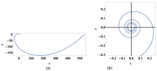
We consider the monoparametric family of orbits in polar coordinates (see spirals in Figure 1a):

$$f(r,\theta )=r{e}^{-\theta }=c,$$

(18)

and

$$\gamma =-r,\alpha ={\displaystyle \frac{r}{2}},\beta =-{\displaystyle \frac{1}{2}}.$$

(19)

Then, we estimate the quantities $\mu ,\nu$ in (11):

$$\mu \left(r\right)=3r,\nu \left(\theta \right)=2.$$

(20)

Using (15), we find the function $A=A\left(r\right)$:

$$A\left(r\right)=-{\displaystyle \frac{b_1}{2r^2}}+{\displaystyle \frac{1}{2}}{d}_{0}logr+b_2.$$

(21)

Using (16), we derive the function $B=B\left(\theta \right)$. The result is

$$B\left(\theta \right)=-{\displaystyle \frac{1}{2}}{d}_0\theta +{\displaystyle \frac{1}{2}}{d}_1{e}^{2\theta }+d_2.$$

(22)

Adding the results (21) and (22), we find the potential function

$$V(r,\theta )=-{\displaystyle \frac{b_1}{2r^2}}+{\displaystyle \frac{1}{2}}{d}_{0}logr-{\displaystyle \frac{1}{2}}{d}_0\theta +{\displaystyle \frac{1}{2}}{d}_1{e}^{2\theta }+g_2,g_2=b_2+d_2,$$

(23)

The energy of the family of orbits (18) is determined. It is:

$$\mathcal{E}={\displaystyle \frac{1}{2}}(2g_2+d_0+d_{0}logc)=const.$$

and c is defined in (1).

Remark 1. 

If we set $b_1=b_2=d_0=d_2=$0 and $d_1=$2 in (23), then we obtain the one-dimensional potential $V=e^{2\theta }$, which was also obtained by ([21], p. 223) and ([4], p. 237).

4. Potentials of the Form $\mathbf{V}=\mathbf{H}\left(\gamma \right)$

In this section, we reconsider Equation (5) and focus our interest on it. We must solve a linear second-order PDE in $V(r,\theta )$, and we seek solutions of the type $V=H\left(\gamma \right)$. Under this assumption the mathematical calculations are made simpler. More precisely, the PDE (5) will be transformed into a second-order ODE, which can be handled more easily than the previous case. Firstly, we compute the partial derivatives of the first and second order of the potential function $V=V(r,\theta )$; then, we substitute them into (5). We have the following:

$$\begin{array}{ccc}\hfill V_r& =& H_{\gamma }{\gamma }_r,V_{\theta }=H_{\gamma }{\gamma }_{\theta },\hfill \\ \hfill V_{rr}& =& H_{\gamma \gamma }{\left({\gamma }_r\right)}^2+H_{\gamma }{\gamma }_{rr},V_{\theta \theta }=H_{\gamma \gamma }{\left({\gamma }_{\theta }\right)}^2+H_{\gamma }{\gamma }_{\theta \theta },V_{r\theta }=H_{\gamma \gamma }{\gamma }_r{\gamma }_{\theta }+H_{\gamma }{\gamma }_{r\theta }\hfill \end{array}$$

(24)

Then, the corresponding Equation (5) reads as follows:

$$J_2{H}_{\gamma \gamma }=-J_1{H}_{\gamma }$$

(25)

where

$$\begin{array}{ccc}\hfill J_2& =& \alpha \gamma {\left({\gamma }_r\right)}^2+(\beta \gamma -\alpha ){\gamma }_r{\gamma }_{\theta }-\beta {\left({\gamma }_{\theta }\right)}^2,\hfill \\ \hfill J_1& =& \alpha \gamma {\gamma }_{rr}+(\beta \gamma -\alpha ){\gamma }_{r\theta }-\beta {\gamma }_{\theta \theta }+\kappa {\gamma }_r+\lambda {\gamma }_{\theta }.\hfill \end{array}$$

(26)

Putting $J_2\ne$ 0, the relation (25) reads

$${\displaystyle \frac{H_{\gamma \gamma }}{H_{\gamma }}}=-{\displaystyle \frac{J_1}{J_2}}.$$

(27)

Since H = $H\left(\gamma \right)$, the ratio $J(r,\theta )=-{\displaystyle \frac{J_1}{J_2}}$ in (27) must be dependent on only the “slope function” $\gamma$. Therefore, we have $J=J\left(\gamma \right(r,\theta \left)\right)$ and

$${\displaystyle \frac{J_r}{J_{\theta }}}={\displaystyle \frac{{\gamma }_r}{{\gamma }_{\theta }}}$$

(28)

or, equivalently,

$${\gamma }_{\theta }{J}_r={\gamma }_r{J}_{\theta }.$$

(29)

Proposition 1. 

It is noteworthy that relation (29) is the necessary and sufficient condition for the “slope function” $\gamma =\gamma (r,\theta )$ as long as Equation (27) has a solution $V=H\left(\gamma \right)$. Indeed, if $\gamma =\gamma (r,\theta )$ is a solution to (29) for which $J_2\ne$ 0, we can find the general solution of (27) analytically.

Having fixed $J=J\left(\gamma \right)$, we proceed as follows. We solve analytically Equation (27), and we obtain

$$H\left(\gamma \right)=c_1\int e^{\int J\left(\gamma \right)d\gamma }d\gamma +c_2$$

(30)

were $c_1,c_2$ are constants and V = $H\left(\gamma \right(r,\theta \left)\right)$. Taking into account (30), we determine the potential function V = $V(r,\theta )$ using quadratures. Therefore, it is important for us to study Equation (29), from which we have the possibility to select appropriate families of orbits $\gamma =\gamma (r,\theta )$, and a compatible potential will be found from (30).

Example 2. 

We regard the monoparametric family of orbits (see spirals in Figure 1b)

$$f(r,\theta )=r(\theta -2)=c,$$

(31)

and

$$\gamma ={\displaystyle \frac{r}{\theta -2}},\alpha ={\displaystyle \frac{r(5-4\theta +{\theta }^2)}{2{(\theta -2)}^2}},\beta ={\displaystyle \frac{5-4\theta +{\theta }^2}{2{(\theta -2)}^3}}.$$

(32)

Then, we determine the ratio $J(r,\theta )=-{\displaystyle \frac{J_1}{J_2}}$ in (27):

$$J(r,\theta )=-{\displaystyle \frac{3}{\gamma }}.$$

(33)

Since $J=J\left(\gamma \right)$, condition (29) is satisfied. Using (30), we find the function $H=H\left(\gamma \right)$:

$$H\left(\gamma \right)=d_2-{\displaystyle \frac{d_1}{2{\gamma }^2}},d_1,d_2=const.$$

(34)

or, equivalently,

$$V(r,\theta )=d_2-{\displaystyle \frac{d_1{(\theta -2)}^2}{2r^2}}.$$

(35)

The energy of the family of orbits (31) is found to be

$$\mathcal{E}=d_2-{\displaystyle \frac{d_1}{2c^2}}=const.$$

5. The Laplace Equation

We consider the well-known Laplace equation in Cartesian coordinates:

$$V_{xx}+V_{yy}=0.$$

(36)

By using the transformation $x=rcos\theta ,y=rsin\theta$, the above equation can be written in polar coordinates:

$$V_{rr}+{\displaystyle \frac{1}{r}}{V}_r+{\displaystyle \frac{1}{r^2}}{V}_{\theta \theta }=0.$$

(37)

Equation (37) cannot be identified with the basic Equation (6). Thus, we select only partial solutions to Equation (37) and look for families of orbits that are compatible with them.

Example 3. 

We start with the partial solution to the Laplace Equation (37), i.e.,

$$V(r,\theta )=k_0(logr+\theta ),k_0=const.$$

(38)

In addition, we select the slope function $\gamma =mr$ where $m\ne$0. We then insert the potential (38) and the corresponding slope function $\gamma =\gamma \left(r\right)$ into (5). This equation gives

$$k_0(m-1)=0.$$

(39)

Thus, Equation (39) is satisfied only for m = 1. Consequently, we have $\gamma =r$. Proceeding further, we use Equation (7), and we find the family of orbits analytically:

$${\displaystyle \frac{d\theta }{dr}}=-{\displaystyle \frac{1}{\gamma (r,\theta )}}=-{\displaystyle \frac{1}{r}},$$

(40)

or, equivalently,

$$\theta +logr=c\iff r{e}^{\theta }=c,c=const.$$

(41)

Example 4. 

In this section, we shall geometrically study similar orbits of the form

$$f=rg\left(\theta \right)=c,$$

(42)

traced by a material point of unit mass. The function $g\left(\theta \right)$ is assumed to be a piecewise analytic $2\pi -$ periodic function of θ. We shall look for homogeneous potentials of degree m, which give rise to this family of orbits, i.e.,

$$V=r^{m}G\left(\theta \right).$$

(43)

In doing so, the Laplace Equation (36) or, equivalently, Equation (37), takes the form

$$r^{m-2}(G^{\prime \prime }\left(\theta \right)+m^{2}G\left(\theta \right))=0.$$

(44)

The general solution to (44) is the following:

$$G\left(\theta \right)=d_{1}cos\left(m\theta \right)+d_{2}sin\left(m\theta \right).$$

(45)

In order to find a suitable pair of orbits that is compatible with the potential (43), we test the monoparametric family of parabolas:

$$f(r,\theta )=r{cos}^2\left({\displaystyle \frac{\theta }{2}}\right)=c.$$

(46)

We insert the expressions (43), (45), and (46) into (5), and we ascertain that this equation is verified for only $m=-{\displaystyle \frac{1}{2}}$. Thus, the potential in (43) takes a simpler form:

$$V(r,\theta )={\displaystyle \frac{d_{1}cos\left(\frac{\theta }{2}\right)+d_{2}sin(-\frac{\theta }{2})}{\sqrt{r}}},$$

(47)

Thus, the energy of the family of orbits (46) is: $\mathcal{E}={\displaystyle \frac{d_1}{2\sqrt{c}}}$.

6. One-Dimensional Potentials

In this section, we shall study one-dimensional potentials of the form $V=A\left(r\right)$ or $V=G\left(\theta \right)$ and find suitable families of orbits produced by them.

6.1. Central Potentials

If we take into account that the potential V depends only on the distance r, i.e., $V=A\left(r\right)$, then Equation (5) takes a simpler form:

$$\alpha \gamma A^{\prime \prime }\left(r\right)+\kappa A^{\prime }\left(r\right)=0.$$

(48)

We define the quantity

$$\mu ={\displaystyle \frac{\kappa }{\alpha \gamma }}.$$

(49)

If $\mu =\mu \left(r\right)$, then we have a solution to our problem, and we find the potential from (49) analytically. We shall give an example for this case.

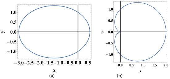
Example 5. 

Consider the monoparametric family of ellipses (see Figure 2a):

$$f(r,\theta )=r(1+{\displaystyle \frac{2}{3}}cos\theta )=c.$$

(50)

Then, Equation (48) reads

$$r{A}^{\prime \prime }\left(r\right)+2A^{\prime }\left(r\right)=0,$$

(51)

Its general solution is the following:

$$A\left(r\right)=-{\displaystyle \frac{d_1}{r}}+d_2,d_1,d_2=const.$$

(52)

For $d_2=0$, we obtain the Newtonian potential $V=-{\displaystyle \frac{d_1}{r}}$. The energy of the family of orbits (50) is given by

$$\mathcal{E}=d_2-{\displaystyle \frac{5d_1}{18c}}.$$

(53)

Other results are shown in

Table 1. Families of orbits produced by central potentials.

Family of Orbits	Potential $\mathit{V}(\mathit{r},\mathit{\theta })$	Energy
$f(r,\theta )=r{e}^{\theta }=c$	$d_2-{\displaystyle \frac{d_1}{r^2}}$	$d_2$
$f(r,\theta )={\displaystyle \frac{r^2}{cos2\theta }}=c$	$d_2-{\displaystyle \frac{d_1}{r^6}}$	$d_2$

.

6.2. Potentials of the Form $V=G\left(\theta \right)$

In this section, we shall examine the second category of one-dimensional potentials, i.e., $V=G\left(\theta \right)$. For this kind of potential, we have the following:

$$V_r=V_{rr}=V_{r\theta }=0.$$

(54)

By using relations (54), Equation (5) takes a simpler form, namely

$$-\beta G^{\prime \prime }\left(\theta \right)+\lambda G^{\prime }\left(\theta \right)=0.$$

(55)

We define the quantity

$$\nu ={\displaystyle \frac{\lambda }{\beta }}.$$

(56)

If $\nu =\nu \left(\theta \right)$, then we have a solution to our problem, and we find the potential from (55) analytically. We shall give an example for this case.

Example 6. 

We study the one-parameter family of cardioids in polar coordinates described as (see Figure 2b)

$$f(r,\theta )={\displaystyle \frac{r}{(1+cos\theta )}}=c,$$

(57)

and

$$\gamma =rtan\left({\displaystyle \frac{\theta }{2}}\right),\alpha ={\displaystyle \frac{r}{3}},\beta ={\displaystyle \frac{1}{3}}tan\left({\displaystyle \frac{\theta }{2}}\right).$$

(58)

Then, quantity ν in (56) has the form

$$\nu \left(\theta \right)=-\left(\right(4+3cos\theta )csc\theta ),$$

(59)

Additionally, Equation (55) reads

$$G^{\prime \prime }\left(\theta \right)+((4+3cos\theta )csc\theta )G^{\prime }\left(\theta \right)=0.$$

(60)

The general solution to (60) is

$$G\left(\theta \right)=d_2-{\displaystyle \frac{1}{24}}{d}_1{csc}^6({\displaystyle \frac{\theta }{2}}),d_1,d_2=const.$$

(61)

The energy of the family of orbits (57) is $\mathcal{E}=d_2$ = const.

Some results are shown in

Table 2. Families of orbits and potentials.

Family of Orbits	Potential $\mathit{V}(\mathit{r},\mathit{\theta })$	Energy
$f(r,\theta )=r{cos}^2{\displaystyle \frac{\theta }{2}}=c$	$d_1+d_{2}cos\theta$	$d_1+d_2$
$f(r,\theta )={\displaystyle \frac{r^2}{cos2\theta }}=c$	${\displaystyle \frac{d_2}{3}}+{\displaystyle \frac{d_1{sec}^3\theta }{{sin}^3\theta }}$	${\displaystyle \frac{d_2}{3}}$

.

7. The Direct Problem

The direct problem of Newtonian Dynamics consists of finding families of orbits $f(r,\theta )=c$ in polar coordinates traced on the $r\theta$ plane by a material point of unit mass under the action of a given potential $V=V(r,\theta )$. In a previous paper [14], the authors studied fourth-order superintegrable systems separating in polar coordinates. Among others, two families of standard superintegrable potentials in $E_2$ are very interesting. Both of them allow for the separation of variables and also admit another polynomial integral of arbitrary order N. For even N, the first one is the well-known Tremblay–Turbiner–Winternitz (TTW) potential ([14]):

$$V_{TTW}=b{r}^2+{\displaystyle \frac{1}{r^2}}\left[{\displaystyle \frac{\overline{\alpha }}{{cos}^2\left(k\theta \right)}}+{\displaystyle \frac{\overline{\beta }}{si{n}^2\left(k\theta \right)}}\right]$$

(62)

where $k=m/n$ and m and n are two integers (with no common divisors). The other one is the Post–Winternitz (PW) potential ([14]):

$$V_{PW}={\displaystyle \frac{a}{r}}+{\displaystyle \frac{1}{r^2}}\left[{\displaystyle \frac{\mu }{{cos}^2\left(\frac{k}{2}\theta \right)}}+{\displaystyle \frac{\nu }{si{n}^2\left(\frac{k}{2}\theta \right)}}\right]$$

(63)

where $k=m/n$ is rational again and $\mu ,\nu$ are constants. For these potentials, we shall find suitable families of orbits compatible with them.

(1)

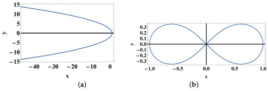
For potential (62), we consider the family of parabolas (see Figure 3a)

$$f(r,\theta )=r{cos}^2\left(k\theta \right)=c,$$

(64)

and

$$\gamma =-2krtan\left(k\theta \right).$$

(65)

We insert these expressions into the basic equation of the problem, i.e., Equation (5), and we ascertain that it is verified for

$$b=0,k={\displaystyle \frac{1}{2}}.$$

Thus, the family of orbits

$$f(r,\theta )=r{cos}^2({\displaystyle \frac{\theta }{2}})=c,$$

(66)

is compatible with the potential

$$V_{TTW}^{*}={\displaystyle \frac{1}{r^2}}\left[{\displaystyle \frac{\overline{\alpha }}{{cos}^2\left(\frac{\theta }{2}\right)}}+{\displaystyle \frac{\overline{\beta }}{si{n}^2\left(\frac{\theta }{2}\right)}}\right],$$

(67)

The energy of the orbits is given by $\mathcal{E}=-{\displaystyle \frac{\overline{\alpha }}{c^2}}$.

Remark 2. 

The potentials appearing in (67) were used by ([5], pp. 377–378) in a study of geometrically similar orbits and for the determination of the families of boundary curves.

(2)

For potential (63), we consider the family of parabolas

$$f(r,\theta )=r{cos}^2(k{\displaystyle \frac{\theta }{2}})=c,$$

(68)

and

$$\gamma =-krtan({\displaystyle \frac{k\theta }{2}}).$$

(69)

We insert these expressions into Equation (5); it is satisfied only for $k=1,-1$. Thus, the family of orbits

$$f(r,\theta )=r{cos}^2({\displaystyle \frac{\theta }{2}})=c,$$

(70)

is compatible with the potential

$$V_{PW}={\displaystyle \frac{a}{r}}+{\displaystyle \frac{1}{r^2}}\left[{\displaystyle \frac{\mu }{{cos}^2\frac{\theta }{2}}}+{\displaystyle \frac{\nu }{si{n}^2\frac{\theta }{2}}}\right],$$

(71)

The energy of the orbits is given by $\mathcal{E}=-{\displaystyle \frac{\mu }{c^2}}$.

Potentials of the Form $V=r^m{sin}^k\left(n\theta \right)$

These are homogeneous potentials of degree m, and $k,n$ are integers. They were used in [2] in order to describe the central bar structure of galaxies, in [4] for the study of geometrically similar orbits and in [7] for the detection of nonintegrability from the same category of orbits.

Example 7. 

We shall examine potentials of the form

$$V(r,\theta )=r^m{sin}^k\left(n\theta \right),k={\displaystyle \frac{2}{n^2}}$$

(72)

For this reason, we consider the monoparametric family of orbits (Bernoulli’s lemniscate, see Figure 3b) given by the equation

$$f(r,\theta )={\displaystyle \frac{r^2}{cos2\theta }}=c,$$

(73)

and

$$\gamma =rtan2\theta ,\alpha ={\displaystyle \frac{r}{6}},\beta ={\displaystyle \frac{1}{6}}tan2\theta .$$

(74)

We insert (72) and (74) into the basic Equation (5) and we find that this equation is verified only for $m=-7$ and $n=2$. Thus, $k={\displaystyle \frac{1}{2}}$. Therefore, the potential V takes the form

$$V(r,\theta )={\displaystyle \frac{\sqrt{sin2\theta }}{r^7}}.$$

(75)

The energy of the family of orbits (73) is found to be $\mathcal{E}=0$.

Working in a similar way for $k=-{\displaystyle \frac{2}{n^2}}$, we find that Equation (5) is satisfied only for $m=-5$ and $n=2$. Thus, $k=-{\displaystyle \frac{1}{2}}$. In this case, the potential is

$$V(r,\theta )={\displaystyle \frac{1}{r^5\sqrt{sin2\theta }}}.$$

(76)

The energy of the family of orbits (73) is found to be $\mathcal{E}=0$.

Remark 3. 

According to [22], the potentials in (75) and (76) are characterized as “adelphic” because they produce the same family of orbits (73).

8. Families of Straight Lines

As was proved by [9], potentials that generate a one-parameter family of straight lines on the $xy$-plane must satisfy the following necessary and sufficient differential condition:

$$\begin{array}{c}\hfill V_x{V}_y(V_{xx}-V_{yy})=V_{xy}(V_x^2-V_y^2).\end{array}$$

(77)

Proceeding with their work, the authors rewrote the above equation in polar coordinates:

$$V_{r\theta }{V}_r^2{r}^3-V_{r\theta }{V}_{\theta }^{2}r-V_{rr}{V}_r{V}_{\theta }{r}^3+V_{\theta \theta }{V}_r{V}_{\theta }r+V_{\theta }^3=0,$$

(78)

and separable potentials of the form $V=A\left(r\right)B\left(\theta \right)$ and circle-producing potentials $V=g\left(r\right)+{\displaystyle \frac{1}{r^2}}h\left(\theta \right)$ that generate families of straight lines on the $r\theta$ plane. In this section, we shall study separable potentials of the form $V=A\left(r\right)+B\left(\theta \right)$, as explored at the beginning of this paper.

If we insert the expression $V=A\left(r\right)+B\left(\theta \right)$ into Equation (78), then we take

$$-A^{″}\left(r\right)A^{\prime }\left(r\right)r^3+B^{″}\left(\theta \right)A^{\prime }\left(r\right)r+{\left[B^{\prime }\left(\theta \right)\right]}^2=0.$$

(79)

Using (79), we shall retrieve solutions for the function $A\left(r\right)$ if and only if we set $B^{\prime }\left(\theta \right)=b$ = const. In doing so, Equation (79) takes the form

$$-A^{″}\left(r\right)A^{\prime }\left(r\right)r^3=-b^2,$$

(80)

or, equivalently,

$${\displaystyle \frac{d}{dr}}{\left[A^{\prime }\left(r\right)\right]}^2={\displaystyle \frac{2b^2}{r^3}}.$$

(81)

If we integrate Equation (81), we obtain

$$A^{\prime }\left(r\right)=\pm \sqrt{c_0-{\displaystyle \frac{b^2}{r^2}}},c_0=const.$$

(82)

Without loss of generality, we take into account the symbol “+” in (82), and we find its general solution as follows:

$$A\left(r\right)=\sqrt{c_0{r}^2-b^2}-barctan\left({\displaystyle \frac{\sqrt{c_0{r}^2-b^2}}{b}}\right).$$

(83)

Taking into account that $B^{\prime }\left(\theta \right)=b$ = const., we conclude that

$$B\left(\theta \right)=b\theta +d_0,d_0=const.$$

(84)

Adding the above results (83) and (84), we find the potential

$$V(r,\theta )=\sqrt{c_0{r}^2-b^2}-barctan\left({\displaystyle \frac{\sqrt{c_0{r}^2-b^2}}{b}}\right)+b\theta +d_0.$$

(85)

9. Conclusions

In this study, we examined four solvable cases of the planar inverse problem of dynamics. We considered monoparametric families of regular orbits $f(r,\theta )=c$ = const. in polar coordinates, which are compatible with the two-dimensional potentials $V=V(r,\theta )$. The general solution to the second-order PDE (5) is not known if a family of orbits $f(r,\theta )=c$ is given in advance. Our aim was to find suitable pairs $\left\{\gamma \right(r,\theta ),V(r,\theta \left)\right\}$ that satisfy the basic Equation (5).

We focused on Equation (5), which is the basic PDE of our problem. We studied four categories of potentials from the studies listed in the References, which provided us with many pieces of information. More precisely, we dealt with separable potentials of the form $V=A\left(r\right)+B\left(\theta \right)$ and provided a pertinent example of spiral orbits compatible with such a potential. Then, we sought solutions to the form $V=H\left(\gamma \right)$. We found necessary and sufficient conditions for the slope function $\gamma =\gamma (r,\theta )$. If these conditions are satisfied for the given slope function $\gamma$, then we have a solution to our problem, and we obtain the potential using quadratures. Proceeding further, we examined potentials that satisfy the Laplace equation in polar coordinates. These potentials are partial solutions to the Laplace equation and produce monoparametric families of orbits on the $r\theta$ plane. Two examples were given here.

The one-dimensional potentials form a special category of potentials and were examined separately. Two cases were investigated: potentials depending on the distance r, i.e., $V=A\left(r\right)$, and potentials depending on the angle $\theta$, i.e., $V=G\left(\theta \right)$. Families of planar orbits produced by them were also found and are presented in Table 1 and Table 2. Another interesting case is the so-called “direct problem” of Newtonian Dynamics. This problem consists of finding families of orbits $f(r,\theta )=c$ if the potential is given in advance. We examined two potentials separable in polar coordinates, the TTW potential and the PW one [14], and a family of potentials that were used for the study of geometrically similar orbits (Section Potentials of the Form $V=r^m{sin}^k\left(n\theta \right)$). Finally, we took into account the case of straight lines and found separable potentials producing them.

This study offers readers a possible solution to handling potentials in polar coordinates and connecting them with the planar inverse problem of dynamics by using the basic equations. The results are completely new and original.

References

- Szebehely, V. On the determination of the potential by satellite observations. In Proceedings of the Convegno Internazionale Sulla Rotazione Della Terra e Osservazioni di Satelliti Artificiali, Cagliari, Italy, 16–18 April 1974; The University of Cagliari Bologna: Cagliari, Italy, 1974; pp. 31–35. [Google Scholar]
- Szebehely, V. Potential in the central bar structure. Astrophys. J. 1980, 239, 880–881. [Google Scholar] [CrossRef][Green Version]
- Ichtiaroglou, S.; Bozis, G. Stability of circular orbits in non-central Newtonian fields. Astron. Astrophys. 1985, 151, 64–68. [Google Scholar]
- Bozis, G.; Stefiades, A. Geometrically similar orbits in homogeneous potentials. Inverse Probl. 1993, 9, 233–240. [Google Scholar] [CrossRef]
- Bozis, G.; Ichtiaroglou, S. Boundary Curves for Families of Planar Orbits. Celest. Mech. Dyn. Astron. 1994, 58, 371–385. [Google Scholar] [CrossRef]
- Bozis, G. The inverse problem of dynamics: Basic facts. Inverse Probl. 1995, 11, 687–708. [Google Scholar] [CrossRef]
- Bozis, G.; Meletlidou, E. Nonintegrability detected from geometrically similar orbits. Celest. Mech. Dyn. Astron. 1998, 68, 335–346. [Google Scholar] [CrossRef]
- Meletlidou, E.; Ichtiaroglou, S. Isolated periodic orbits and stability in separable potentials. Celest. Mech. Dyn. Astron. 1999, 71, 289–300. [Google Scholar] [CrossRef]
- Bozis, G.; Anisiu, M.-C. Families of straight lines in planar potentials. Rom. Astron. J. 2001, 11, 27–43. [Google Scholar]
- Bozis, G.; Anisiu, M.-C. A solvable version of the inverse problem of dynamics. Inverse Probl. 2005, 21, 487–497. [Google Scholar] [CrossRef]
- Kotoulas, T. Monoparametric families of orbits produced by planar potentials. Axioms 2023, 12, 423. [Google Scholar] [CrossRef]
- Borghero, F.; Demontis, F. Three-dimensional inverse problem of geometrical optics: A mathematical comparison between Fermat’s principle and the eikonal equation. JOSA A 2016, 33, 1710. [Google Scholar] [CrossRef] [PubMed]
- Escobar-Ruiz, M.A.; López Vieyra, J.C.; Winternitz, P. Fourth-order superintegrable systems separating in polar coordinates. I. Exotic potentials. J. Phys. A Math. Ther. 2018, 49, 495206. [Google Scholar] [CrossRef]
- Escobar-Ruiz, M.A.; López Vieyra, J.C.; Winternitz, P.; Yurduşen, İ. Fourth-order superintegrable systems separating in polar coordinates. II.Standard potentials. J. Phys. A Math. Ther. 2018, 51, 40LT01. [Google Scholar] [CrossRef]
- Escobar-Ruiz, M.A.; López Vieyra, J.C.; Winternitz, P.; Yurduşen, İ. General Nth-order superintegrable systems separating in polar coordinates. J. Phys. A Math. Ther. 2018, 51, 455202. [Google Scholar] [CrossRef]
- DeCosta, R.; Altschul, B. Separability of the Planar 1ρ2 Potential in Multiple Coordinate Systems. Symmetry 2020, 12, 1312. [Google Scholar] [CrossRef]
- Kravchenko, V.V.; Torba, S.M. A direct method for solving inverse Sturm–Liouville problems. Inverse Probl. 2021, 37, 015015. [Google Scholar] [CrossRef]
- Mitsopoulos, A.; Tsamparlis, M. Integrable and Superintegrable 3D Newtonian Potentials Using Quadratic First Integrals: A Review. Universe 2023, 9, 22. [Google Scholar] [CrossRef]
- Dragas, M.; Galovic, S.; Milicevic, D.; Suljovrujic, E.; Djordjevic, K. Solution of Inverse Photoacoustic Problem for Semiconductors via Phase Neural Network. Mathematics 2024, 12, 2858. [Google Scholar] [CrossRef]
- Ichtiaroglou, S.; Meletlidou, E. On monoparametric families of orbits sufficient for integrability of planar potentials with linear or quadratic invariants. J. Phys. A Math. Gen. 1990, 23, 3673–3679. [Google Scholar] [CrossRef]
- Broucke, R.; Lass, H. On Szebehely’s equation for the potential of a prescribed family of orbits. Celest. Mech. 1977, 16, 215–225. [Google Scholar] [CrossRef]
- Bozis, G. Adelphic potentials. Astron. Astrophys. 1986, 160, 107–110. [Google Scholar]
Disclaimer/Publisher’s Note: The statements, opinions and data contained in all publications are solely those of the individual author(s) and contributor(s) and not of MDPI and/or the editor(s). MDPI and/or the editor(s) disclaim responsibility for any injury to people or property resulting from any ideas, methods, instructions or products referred to in the content. |
© 2024 by the author. Licensee MDPI, Basel, Switzerland. This article is an open access article distributed under the terms and conditions of the Creative Commons Attribution (CC BY) license (https://creativecommons.org/licenses/by/4.0/).