A Bimodal Exponential Regression Model for Analyzing Dengue Fever Case Rates in the Federal District of Brazil

Abstract

Dengue fever remains a significant epidemiological challenge globally, particularly in Brazil, where recurring outbreaks strain healthcare systems. Traditional statistical models often struggle to accurately capture the complexities of dengue case distributions, especially when data exhibit bimodal patterns. This study introduces a novel bimodal regression model based on the log-generalized odd log-logistic exponential distribution, offering enhanced flexibility and precision for analyzing epidemiological data. By effectively addressing multimodal distributions, the proposed model overcomes the limitations of unimodal models, making it well suited for public health applications. Through regression analysis of dengue case data from the Federal District of Brazil during the epidemiological weeks of 2022, the model demonstrates its capacity to improve the fit of the disease rate. The model’s parameters are estimated using maximum likelihood estimation, and Monte Carlo simulations validate their accuracy. Additionally, local influence measures and residual analysis ensure the proposed model’s goodness-of-fit. While this innovative regression model offers substantial advantages, its effectiveness depends on the availability of high-quality data, and further validation is necessary to confirm its applicability across diverse diseases and regions with varying epidemiological characteristics.

1. Introduction

Dengue fever presents a major challenge to epidemiology worldwide, especially in Brazil, where recurring epidemics occur in certain endemic regions. The rapid, uncontrolled growth of metropolitan populations and the lack of awareness and preventive measures are factors that contribute to the spread of the disease and place a significant burden on the healthcare system. More than 100 countries face dengue fever as an endemic issue, affecting millions of people globally each year. One of the most critical factors driving the current global spread of the virus is the rapidly accelerating climate change. Lately, ref. [1] proposed a novel class of discrete distributions and examined eight different datasets illustrating mortality, infection, and medication statistics. The results demonstrated its superiority over typical discrete modeling options in terms of model fit and flexibility, particularly in handling heavy-tailed datasets. In this context, numerous applications of generalized extreme value (GEV) distributions can be found in epidemiological studies. Ref. [2] presented a review of the relationship between dengue fever and meteorological parameters, along with a meta-analysis investigating the impact of ambient temperature and precipitation. In [3], dengue case counts during outbreaks in Thailand were modeled using extreme value theory (EVT). A zero-inflated GEV regression model is applied to the Vietnam dengue data in [4], estimating the infection risk for individuals based on covariates such as age and weight. In a related study, ref. [5] presented a GEV approach to investigate the frequency and intensity of extreme novel epidemics, including those similar to COVID-19. Extreme value statistics have also been used to predict severe influenza epidemics in real time [6]. Additionally, ref. [7] explored the extreme correlation between infectious disease outbreaks and crude oil futures. Finally, ref. [8] estimated the disease burden of dengue in endemic regions to analyze the influence of socioeconomic factors. It is recommended to allocate more resources to areas with high population expansion and urbanization. Furthermore, ref. [9] explored the characteristics and studied the temporal–spatial distribution of overseas imported dengue fever cases in outbreak provinces of China. Ref. [10] conducted a systematic review on myocardial manifestations related to dengue fever cases. In [11], dengue fever cases in the Brazilian state of Alagoas were modeled monthly using the GEV distribution. The findings underscore the importance of ongoing monitoring and assistance in this area. Therefore, this study focuses on dengue fever cases during the epidemiological weeks of 2022 in the Federal District of Brazil. Regression analysis is applied to study extreme events (epidemiological events that affect health centers and the economy), and the maximum likelihood method is used to estimate the parameters. The accuracy of the estimators is confirmed through Monte Carlo simulations. Local influence measures and residual analyses are employed to validate the goodness-of-fit of the proposed model.

The study introduces a new bimodal regression model based on the generalized odd log-logistic exponential (GOLLE) distribution. The broad flexibility of the generalized odd log-logistic (GOLL-G) class, which allows for modeling both its tails and skewness, combined with the exponential distribution’s closed mathematical form, makes this novel regression model highly relevant for applications in many fields, including the analysis of extreme events. Traditional models often fail to capture environmental and socioeconomic variations, especially when the data is bimodal. Consequently, this model is particularly innovative, as it provides a more accurate fit for data that deviate from the assumptions of unimodal models. It is specifically designed to analyze epidemiological data with multimodal patterns in case rates and holds potential for use in public health contexts. Given this, the novel LGOLLE regression model has the potential to enhance accuracy in estimating disease case rates, leading to more timely public health decisions for prevention or treatment. However, while the model offers many advantages, it may require high-quality data, which could be a limitation in some cases. Additionally, its applicability to other diseases or regions with different epidemiological factors would require further validation.

The remaining work is organized as follows: Section 2 presents the GOLLE distribution, as discussed in [12,13]. It also explores the linear representation and its mathematical properties. The maximum likelihood estimate (MLE) is explained, along with a Monte Carlo simulation analysis demonstrating the estimators’ consistency. Section 3 introduces the new LGOLLE distribution, employs maximum likelihood estimation, and conducts simulations to evaluate the MLEs’ consistency. A novel regression model based on the LGOLLE distribution is proposed, incorporating location parametrization. Simulations are performed to investigate the behavior of the estimates, and the model’s fit is evaluated using global influence measures and residual analysis. Section 4 applies the novel regression model to epidemiological data, presenting findings and comments. Finally, Section 5 offers concluding remarks.

2. Materials and Methods

Recently, the development of new distributions based on well-known ones has aimed to better capture the underlying distribution of the data, leading to more precise estimates of key quantities of interest.

The GOLL-G family, introduced by [14], is a versatile class of continuous distributions that can effectively model various types of data. The study demonstrated the advantages of this family, highlighting its flexibility in fitting skewed, bimodal, and asymmetric data sets, as well as its ability to capture a wide range of hazard function shapes. Ref. [15] developed a novel bimodal normal regression model based on the GOLLN distribution to assess patients’ survival time in the intensive care unit due to COVID-19 in a Brazilian hospital. Additionally, Ref. [16] investigated factors influencing county-level COVID-19 vaccination rates in Texas, United States, using the GOLLL regression model.

This class of distributions is based on the transformer-transformer (T-X) generator defined by [17]. Consider a baseline cumulative distribution function (cdf) $G\left(x\right)=G(x;\mathit{\xi })$, where $\mathit{\xi }$ denotes an unknown parameter vector. The GOLL-G cdf is defined by integrating the log-logistic density function, namely

$$F\left(y\right)={\int }_0^{{\displaystyle \frac{G{\left(x\right)}^{\theta }}{1-G{\left(x\right)}^{\theta }}}}{\displaystyle \frac{\alpha w^{\alpha -1}}{{(1-w)}^2}}dw={\displaystyle \frac{G{\left(x\right)}^{\alpha \theta }}{G{\left(x\right)}^{\alpha \theta }+{[1-G{\left(x\right)}^{\theta }]}^{\alpha }}},$$

(1)

where $\alpha$ > 0 and $\theta$ > 0 are two extra shape parameters.

The probability density function (pdf) corresponding to (1) can be expressed as

$$f\left(y\right)={\displaystyle \frac{\alpha \theta g\left(x\right)G{\left(x\right)}^{\alpha \theta -1}{[1-G{\left(x\right)}^{\theta }]}^{\alpha -1}}{{\{G{\left(x\right)}^{\alpha \theta }+{[1-G{\left(x\right)}^{\theta }]}^{\alpha }\}}^2}},$$

(2)

where $g\left(x\right)=g(x;\xi )$ is the baseline pdf.

These equations define key characteristics of the GOLL-G family, allowing it to effectively model a wide range of data types. The extra parameters $\alpha$ and $\theta$ are crucial in shaping the distribution.

Table 1. Sub-models of the GOLL-G family of distributions.

$\mathit{\alpha }$	$\mathit{\theta }$	Sub-Model
-	1	Generalized log-logistic family [18]
1	-	Proportional reversed hazard rate family [19]
1	1	Baseline

reports several sub-models of Equation (1).

The cdf and the pdf of the GOLLE distribution are defined in [12,13], respectively, inserting the cdf and the pdf of the exponential distribution, $G(y;\lambda )$, into Equations (1) and (2), as follows (for $y>0$)

$$F(y;\alpha ,\theta ,\lambda )={\displaystyle \frac{{\left(1-{\mathrm{e}}^{-\lambda y}\right)}^{\alpha \theta }}{{\left(1-{\mathrm{e}}^{-\lambda y}\right)}^{\alpha \theta }+{\left[1-{\left(1-{\mathrm{e}}^{-\lambda y}\right)}^{\theta }\right]}^{\alpha }}}$$

(3)

and

$$f(y;\alpha ,\theta ,\lambda )={\displaystyle \frac{\alpha \theta \lambda {\mathrm{e}}^{-\lambda y}{\left(1-{\mathrm{e}}^{-\lambda y}\right)}^{\alpha \theta -1}{\left[1-{\left(1-{\mathrm{e}}^{-\lambda y}\right)}^{\theta }\right]}^{\alpha -1}}{{\left\{{\left(1-{\mathrm{e}}^{-\lambda y}\right)}^{\alpha \theta }+{\left[1-{\left(1-{\mathrm{e}}^{-\lambda y}\right)}^{\theta }\right]}^{\alpha }\right\}}^2}},$$

(4)

where $\alpha ,\theta ,\lambda >0$.

The corresponding hrf ($\tau \left(y\right)=f\left(y\right)/[1-F(y\left)\right]$) is easily determined as

$$\tau (y;\alpha ,\theta ,\lambda )={\displaystyle \frac{\alpha \theta \left(\lambda {\mathrm{e}}^{-\lambda x}\right){\left(1-{\mathrm{e}}^{-\lambda x}\right)}^{\alpha \theta -1}}{\left[1-{\left(1-{\mathrm{e}}^{-\lambda x}\right)}^{\theta }\right]\left\{{\left(1-{\mathrm{e}}^{-\lambda x}\right)}^{\alpha \theta }+{[1-{\left(1-{\mathrm{e}}^{-\lambda x}\right)}^{\theta }]}^{\alpha }\right\}}}.$$

(5)

In addition, Equations (3) and (4) do not involve complex mathematical functions, unlike the gamma and beta distributions. In

Table 2. Sub-models of the GOLLE distribution.

$\mathit{\alpha }$	$\mathit{\theta }$	Sub-Model
-	1	Odd log-logistic exponential (OLLE) distribution, see [18]
1	-	Exponentiated-exponential (EE) distribution, see [20]
1	1	Exponential (E) distribution

, the sub-models obtained from Equation (4) are presented. Their ability to handle data fitting across a wide range of distributions demonstrates their versatility and applicability.

Figure 1 and Figure 2 show plots of the Y’s hrfs and histograms for selected parameters. One of the most notable properties of the GOLLE distribution is its ability to generate a wide range of hazard shapes, in contrast to the exponential hrf’s constant behavior over time. Figure 1 illustrates many forms, including the inverse J-shape, increasing–decreasing, decreasing–increasing and bathtub. Figure 2 demonstrates that the model is effective for modeling non-normal data sets with diverse histogram patterns (e.g., asymmetric, heavy-tailed, multimodal).

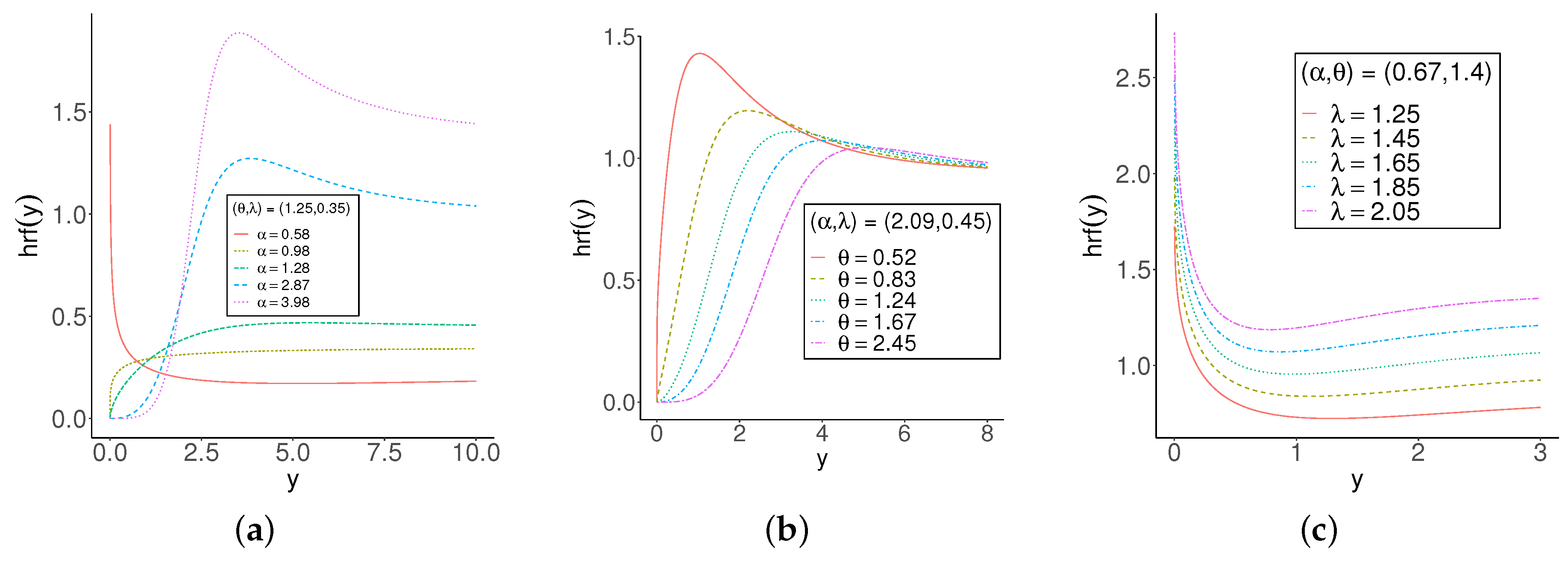
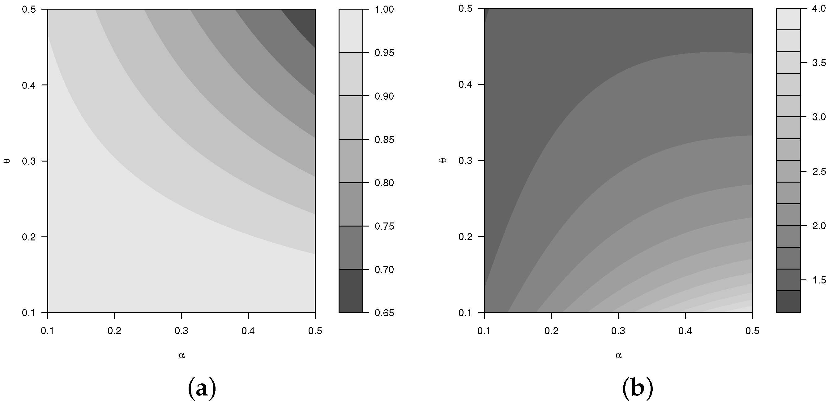
2.1. Main Properties

This Section reviews the linear representation of the GOLLE distribution’s density function, including the quantile function (qf), moments, and the moment generating function (mgf), as shown in [13].

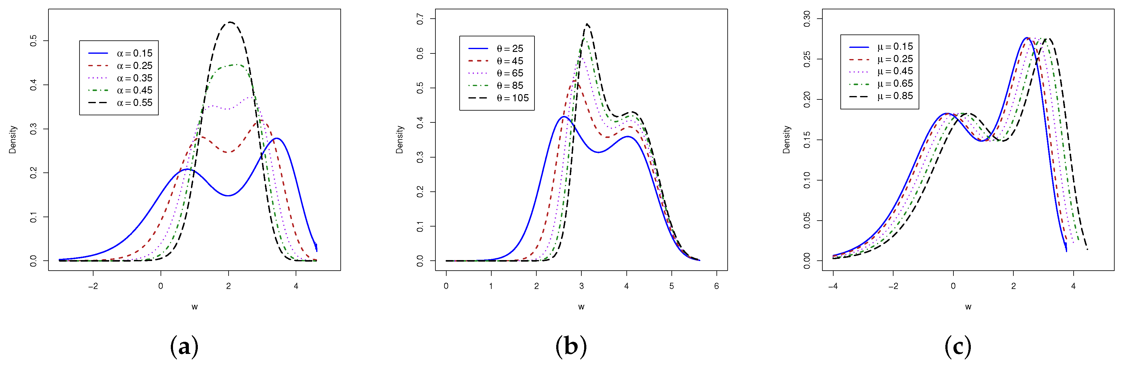
2.1.1. Representation

Definition 1. 

The GOLLE density (4) can be represented linearly using exponential densities as

$$f(y;\alpha ,\theta ,{\lambda }^{*})=\sum _{k,m=0}^{\infty }{h}_{k,m}g(y;{\lambda }^{*}),$$

(6)

where $g(·)$ is the exponential density with a shared parameter ${\lambda }^{*}={\lambda }^{*}(\lambda ,m)=\lambda (m+1)$ and $h_{k,m}$ is defined below

$$h_{k,m}={\displaystyle \frac{{(-1)}^m(k+1)\left(\genfrac{}{}{0pt}{}{k}{m}\right)}{(m+1)}}{b}_k.$$

2.1.2. Quantile Function

Definition 2. 

The GOLLE qf of Y, used to simulate the density, is expressed by

$$Q\left(u\right)=-{\displaystyle \frac{1}{\lambda }}log[1-{\epsilon }_{\alpha .\theta }\left(u\right)],$$

(7)

where

$${\epsilon }_{\alpha ,\theta }\left(u\right)={\left[{\displaystyle \frac{{\left(\frac{u}{1-u}\right)}^{1/\alpha }}{1+{\left(\frac{u}{1-u}\right)}^{1/\alpha }}}\right]}^{1/\theta }.$$

Figure 3 displays Galton’s skewness and Moors’ kurtosis for different $\alpha$ and $\theta$, with $\lambda =1.58$. These plots illustrate that as the parameter $\alpha$ increases, the distribution becomes more right-skewed and leptokurtic, eventually reaching a minimum value.

2.1.3. Moments

Definition 3. 

The nth moment of the GOLLE distribution is defined by

$${\mu }_n^{\prime }=E\left(Y^n\right)=\sum _{k,m=0}^{\infty }{\displaystyle \frac{1}{{\lambda }^{*}}}{h}_{k,m}=\sum _{k,m=0}^{\infty }{\displaystyle \frac{{(-1)}^m(k+1)\left(\genfrac{}{}{0pt}{}{k}{m}\right)}{(m+1){\lambda }^{*}}}{b}_k.$$

2.1.4. Generating Function

Definition 4. 

The mgf of the GOLLE density can be expressed as

$$M_Y\left(t\right)=\sum _{k,m=0}^{\infty }{\displaystyle \frac{{\lambda }^{*}}{{\lambda }^{*}-t}}{h}_{k,m}=\sum _{k,m=0}^{\infty }{\displaystyle \frac{{(-1)}^m(k+1){\lambda }^{*}}{{\lambda }^{*}-t}}{b}_k,t<{\lambda }^{*}.$$

2.1.5. Estimation

The MLEs of the GOLLE parameters vector $\mathit{\psi }={(\alpha ,\theta ,\lambda )}^{\top }$ are calculated from a complete sample $y_1,\dots ,y_n$ of the Equation (4) by maximizing the log-likelihood function

$$\begin{array}{cc}\hfill {\mathcal{L}}_n\left(\mathit{\psi }\right)& =nlog\left(\alpha \theta \lambda \right)-\lambda \sum _{i=1}^n{y}_i+(\alpha \theta -1)\sum _{i=1}^{n}log(1-{\mathrm{e}}^{-\lambda y_i})+(\alpha -1)\sum _{i=1}^{n}log\left[1-{(1-{\mathrm{e}}^{-\lambda y_i})}^{\theta }\right]\hfill \\ \hfill & -2\sum _{i=1}^{n}log\left\{{(1-{\mathrm{e}}^{-\lambda y_i})}^{\alpha \theta }+{\left[1-{(1-{\mathrm{e}}^{-\lambda y_i})}^{\theta }\right]}^{\alpha }\right\}.\hfill \end{array}$$

(8)

Let’s consider

$$A_i\left(\lambda \right)=A_i=1-{\mathrm{e}}^{\lambda y_i}.$$

Therefore, the elements of the score vector can be formulated as follows

$$\begin{array}{ccc}\hfill U_{\alpha }& =& {\displaystyle \frac{n}{\alpha }}+\theta \sum _{i=1}^{n}log\left(A_i\right)+\sum _{i=1}^{n}log\left(1-{A_i}^{\theta }\right)\hfill \\ & -& 2\sum _{i=1}^n{\displaystyle \frac{\theta log\left(A_i\right){A_i}^{\alpha \theta }+{(1-{A_i}^{\theta })}^{\alpha }log(1-{A_i}^{\theta })}{{A_i}^{\alpha \theta }+{(1-{A_i}^{\theta })}^{\alpha }}},\hfill \end{array}$$

$$\begin{array}{ccc}\hfill U_{\theta }& =& {\displaystyle \frac{n}{\theta }}+\alpha \sum _{i=1}^{n}log\left(A_i\right)-(\alpha -1)\sum _{i=1}^n{\displaystyle \frac{{A_i}^{\theta }log\left(A_i\right)}{1-{A_i}^{\theta }}}\hfill \\ & +& \sum _{i=1}^n{\displaystyle \frac{\alpha {A_i}^{\alpha \theta }log\left(A_i\right)+{(1-{A_i}^{\alpha })}^{\theta }log(1-{A_i}^{\alpha })}{{A_i}^{\alpha \theta }+{(1-{A_i}^{\alpha })}^{\theta }}},\hfill \end{array}$$

and

$$\begin{array}{ccc}\hfill U_{\lambda }& =& {\displaystyle \frac{n}{\lambda }}-\sum _{i=1}^n{y}_i+(\alpha \theta -1)\sum _{i=1}^n{\displaystyle \frac{(1-A_i)}{A_i}}-\theta (\alpha -1)\sum _{i=1}^n{\displaystyle \frac{(1-A_i)A_i^{\theta -1}}{1-A_i^{\theta }}}\hfill \\ & -& 2\alpha \theta \sum _{i=1}^n{\displaystyle \frac{(1-A_i)[A_i^{\alpha \theta -1}-A_i^{\theta -1}{(1-A_i^{\theta })}^{\alpha -1}]}{A_i^{\alpha \theta }+{(1-A_i^{\theta })}^{\alpha }}}.\hfill \end{array}$$

Using a Newton–Raphson type method and setting the score equations $U_{\alpha }=U_{\theta }=U_{\lambda }=0$, the MLEs can be calculated. Due to the complexity of the equations for the GOLLE model, analytical solutions are generally not feasible. Therefore, numerical optimization techniques are employed to solve these equations. The Broyden–Fletcher–Goldfarb–Shanno (BFGS) algorithm, implemented through the optim function in [21] (version 4.4.1), is used to maximize Equation (8). This method is well-suited for maximizing complex likelihood functions due to its balance between computational efficiency and robustness.

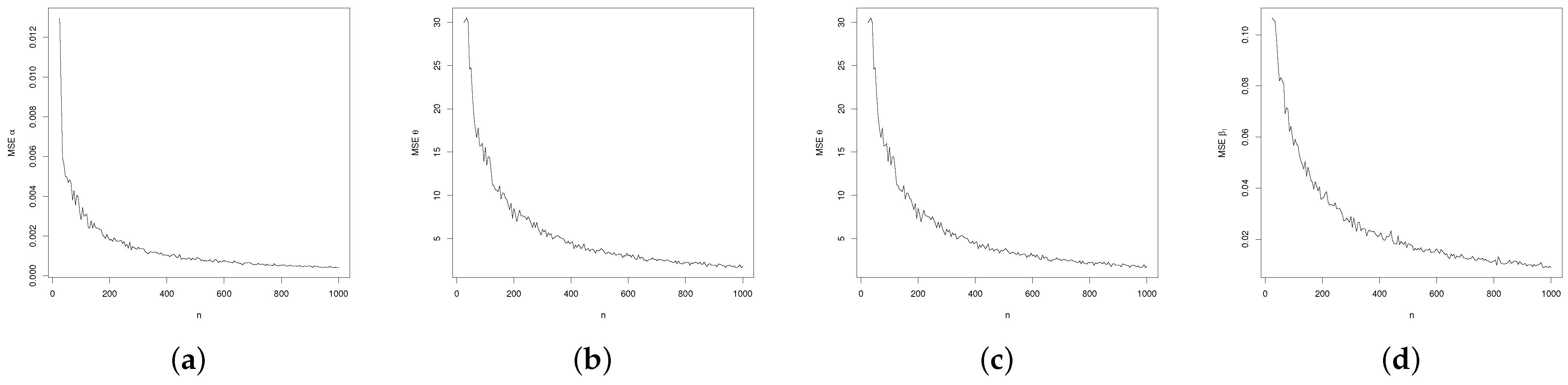
2.1.6. Simulation Study

In two scenarios, based on the settings depicted in Figure 1c and Figure 2b, Monte Carlo simulations were generated by 1000 samples of varying sizes from the GOLLE distribution are utilized to assess the accuracy of MLEs. For each sample size, $n=\{50,150,300,500,750,1000\}$, the average estimates (AEs), absolute biases (ABs), and root mean square errors (RMSEs) are computed, for each $(\alpha ,\theta ,\lambda )$ (

Table 3. Simulations results for GOLLE distribution for scenario 1.

Scenario 1—GOLLE (0.67, 1.40, 1.25)
Par	n = 50			n = 150			n = 300
	AE	AB	RMSE	AE	AB	RMSE	AE	AB	RMSE
$\alpha$	0.817	0.147	0.750	0.742	0.072	0.381	0.724	0.054	0.292
$\theta$	2.609	1.209	3.157	1.756	0.356	1.194	1.557	0.157	0.728
$\lambda$	1.729	0.479	1.364	1.393	0.143	0.713	1.307	0.057	0.508
Par	n = 500			n = 750			n = 1000
$\alpha$	0.707	0.037	0.212	0.676	0.006	0.155	0.681	0.011	0.135
$\theta$	1.477	0.077	0.537	1.496	0.096	0.433	1.452	0.052	0.351
$\lambda$	1.269	0.019	0.392	1.301	0.051	0.317	1.273	0.023	0.267

and

Table 4. Simulations results for GOLLE distribution for scenario 2.

Scenario 2—GOLLE (0.22, 1.13, 7.50)
Par	n = 50			n = 150			n = 300
$\alpha$	0.261	0.041	0.185	0.240	0.020	0.104	0.231	0.011	0.063
$\theta$	1.413	0.283	0.877	1.212	0.082	0.465	1.151	0.021	0.308
$\lambda$	9.167	1.667	5.438	7.954	0.454	2.990	7.655	0.155	2.206
Par	n = 500			n = 750			n = 1000
$\alpha$	0.223	0.003	0.044	0.224	0.004	0.040	0.222	0.002	0.030
$\theta$	1.155	0.025	0.223	1.141	0.011	0.197	1.141	0.011	0.156
$\lambda$	7.625	0.125	1.448	7.577	0.077	1.214	7.589	0.089	1.008

).

As predicted by the consistency requirement, the results in Table 3 and Table 4 indicate that AEs approximate the real values and ABs and RMSE approach zero as n increases. It is notable that for scenario 1, all the estimates obtained when $n=50$ were overestimated, while for scenario 2, the parameters $\theta$ and $\lambda$ were overestimated. This shows the sensitivity of the model’s parameters to some values, but in general, as the sample size increases, convergence towards the true values is achieved.

3. The Proposal LGOLLE Distribution

The LGOLLE distribution is proposed to address particular problems that arise when studying epidemiological data, especially in cases like dengue disease, where the data contains bimodal distributions. Traditional models usually use a unimodal distribution, which may not accurately reflect the complexity of the actual data.

Let Y be a random variable (rv) following the GOLLE density function (4). Define $W=log\left(Y\right)$. Setting $\lambda =-{\mathrm{e}}^{\mu }$, the density function of W is expressed as (for $y\in \mathbb{R}$)

$$f(y;\alpha ,\theta ,\mu )={\displaystyle \frac{\alpha \theta {\mathrm{e}}^{[(y-\mu )-{\mathrm{e}}^{y-\mu }]}{\left[1-{\mathrm{e}}^{-{\mathrm{e}}^{y-\mu }}\right]}^{\alpha \theta -1}{\left[1-{\left(1-{\mathrm{e}}^{-{\mathrm{e}}^{y-\mu }}\right)}^{\theta }\right]}^{\alpha -1}}{{\left\{{\left(1-{\mathrm{e}}^{-{\mathrm{e}}^{y-\mu }}\right)}^{\alpha \theta }+{\left[1-{\left(1-{\mathrm{e}}^{-{\mathrm{e}}^{y-\mu }}\right)}^{\theta }\right]}^{\alpha }\right\}}^2}},$$

(9)

where $\mu \in \mathbb{R}$.

The Equation (9) represents the LGOLLE distribution, denoted as $W\sim$ LGOLLE($y;\alpha ,\theta ,\mu$), where $\mu$ is the location parameter. Thus, if $Y\sim$ GOLLE($y;\alpha ,\theta$) then $W=log\left(Y\right)\sim$ LGOLLE($y;\alpha ,\theta ,\mu$). The density function in Figure 4 is displayed for selected values of the parameters $\alpha ,\theta$, and $\mu$. These plots illustrate the versatility of the new distribution, demonstrating its skewed and bimodal shapes.

3.1. The New LGOLLE Regression Model

The novel regression model has wide potential in public health, notably, for epidemiologists, policymakers, and data scientists. The model’s capacity to handle bimodal distributions enables more accurate predictions in complex epidemiological scenarios, making it a viable option for applications beyond dengue fever. While the recently developed regression model is relevant for diseases with bimodal distributions, it is essential to expand its application to more conditions or diseases for further validation.

Thus, let be $W\sim$ LGOLLE($\alpha ,\theta ,\mu$) the density function, thus the rv $Z=Y-\mu$ is given by

$$f(z;\alpha ,\theta ,\mu )={\displaystyle \frac{\alpha \theta {\mathrm{e}}^{[z-{\mathrm{e}}^z]}{\left[1-{\mathrm{e}}^{-{\mathrm{e}}^z}\right]}^{\alpha \theta -1}{\left[1-{\left(1-{\mathrm{e}}^{-{\mathrm{e}}^z}\right)}^{\theta }\right]}^{\alpha -1}}{{\left\{{\left(1-{\mathrm{e}}^{-{\mathrm{e}}^z}\right)}^{\alpha \theta }+{\left[1-{\left(1-{\mathrm{e}}^{-{\mathrm{e}}^z}\right)}^{\theta }\right]}^{\alpha }\right\}}^2}},$$

(10)

and the rv $Z\sim$ LGOLLE($\alpha ,\theta$,0).

In order to introduce a new regression structure in the class of models (10), the parameter ${\mu }_i$ is assumed to vary across observations through a regression structure expressed as

$$y_i={\mu }_i+z_i,i=1,\dots ,n,$$

(11)

where the random error $z_i$ has density function (10) and ${\mu }_i$ is parameterized by

$${\mu }_i={\mu }_i\left({\mathit{x}}_{\mathit{i}}^{\top }\mathit{\beta }\right),$$

where $\mathit{\beta }={(\beta ,\dots ,{\beta }_p)}^{\top }$ is the parameter vector of dimension p associated with the explanatory variables ${\mathit{x}}_{\mathit{i}}^{\top }=(x_{i1},\dots ,x_{ip})$ for the location parameter.

3.2. Estimation

Except for ${\mu }_i$, the components of the score vector for $U_{\alpha }$ and $U_{\theta }$ are the same as those obtained from the Equations presented in Section 2.1.5. The score component of the location parameter ${\mu }_i$ is defined to add the regression part as follows

$$\begin{array}{ccc}\hfill U_{{\mu }_i}& =& \sum _{i=1}^{\infty }{\displaystyle \frac{{\partial }_{\mathit{\beta }}f(z_i;{\mu }_i)}{f(z_i;{\mu }_i)}}+(\alpha \theta -1)\sum _{i=1}^{\infty }{\displaystyle \frac{{\partial }_{\mathit{\beta }}F(z_i;{\mu }_i)}{F(z_i;{\mu }_i)}}+\theta (1-\alpha )\sum _{i=1}^{\infty }{\displaystyle \frac{{\partial }_{\mathit{\beta }}F(z_i;{\mu }_i)GF{z}_i;{\mu }_i{)}^{\theta -1}}{1-F{(z_i;{\mu }_i)}^{\theta }}}\hfill \\ & -& 2\sum _{i=1}^{\infty }{\partial }_{\mathit{\beta }}F(z_i;{\mu }_i){\displaystyle \frac{F{(z_i;{\mu }_i)}^{\alpha \theta -1}-F{(z_i;{\mu }_i)}^{\theta -1}{[1-F{(z_i;{\mu }_i)}^{\theta }]}^{\alpha -1}}{F{(z_i;{\mu }_i)}^{\alpha \theta }+{[1-F{(z_i;{\mu }_i)}^{\theta }]}^{\alpha }}},\hfill \end{array}$$

where $F(·)$ and $f(·)$ are the cdf and pdf of the exponential distribution, respectively, ${\partial }_{\mathit{\beta }}f(z_i;{\mu }_i)={\partial }_{{\mu }_i}f(z_i;{\mu }_i){\partial }_{\mathit{\beta }}{\mu }_i(z_i;\mathit{\beta })$ and ${\partial }_{\mathit{\beta }}F(z_i;{\mu }_i)={\partial }_{{\mu }_i}F(z_i;{\mu }_i){\partial }_{\mathit{\beta }}{\mu }_i(z_i;\mathit{\beta })$ denotes the derivatives of the parameter ${\mu }_i$ using the chain rule.

The MLE $\widehat{\mathit{\psi }}$ of $\mathit{\psi }$ of the regression model is calculated either by setting the score equations $U_{\alpha }=U_{\theta }=U_{{\mu }_i}=0$ or using the optim routine in [21] (version 4.4.1).

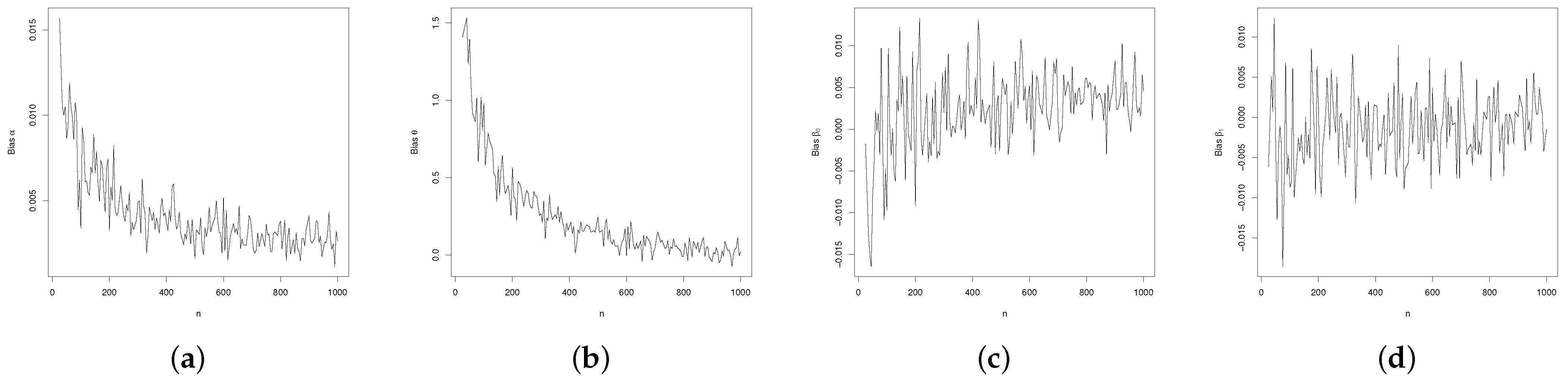
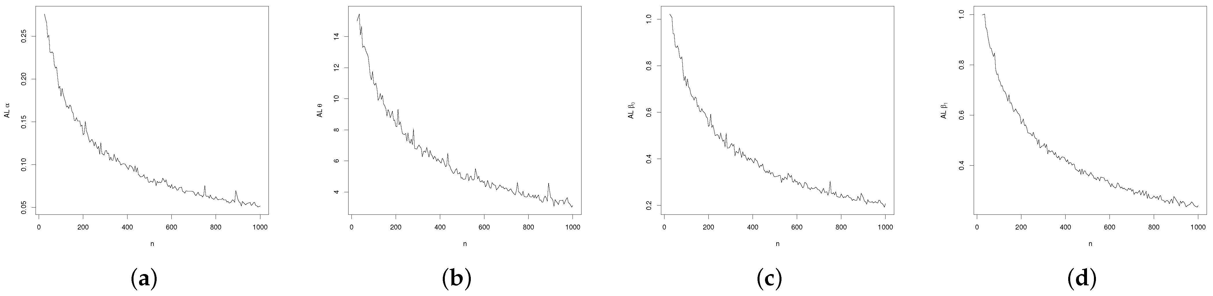
3.3. Regression Simulation Study

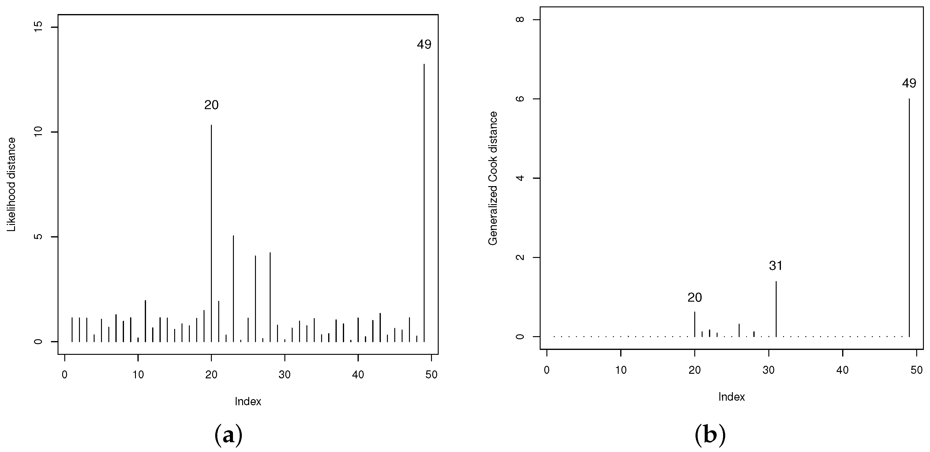
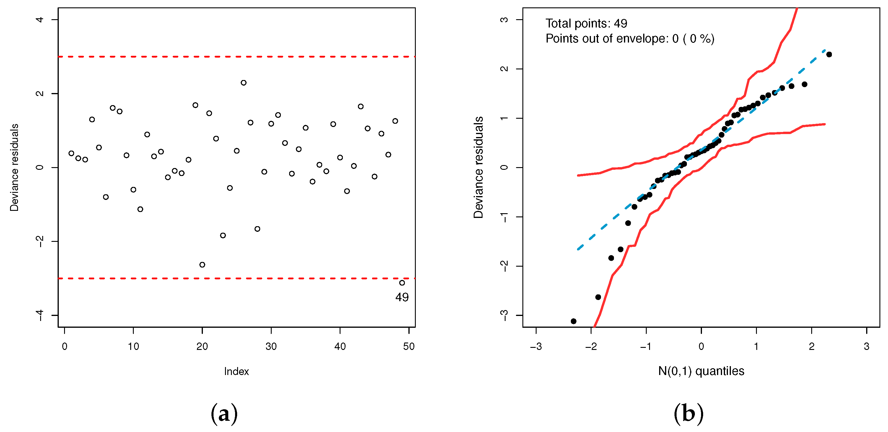
To show the accuracy of the MLEs for $\alpha =0.25$, $\theta =9.75$, ${\beta }_0=0.89$, and ${\beta }_1=1.15$, 1000 samples of size $n=\{25,\dots ,1000\}$ were generated. The study is based on the following measurements: biases, mean square errors (MSEs), and average lengths (ALs). The measures are (for $ϵ=\alpha ,\theta ,\lambda$)

$$Bia{s}_{ϵ}\left(n\right)={\displaystyle \frac{1}{N}}\sum _{i=1}^N({\widehat{ϵ}}_i-ϵ),MS{E}_{ϵ}\left(n\right)={\displaystyle \frac{1}{N}}\sum _{i=1}^N{({\widehat{ϵ}}_i-ϵ)}^2\mathrm{and}A{L}_{ϵ}\left(n\right)={\displaystyle \frac{3.919928}{N}}\sum _{i=1}^N{s}_{{\widehat{ϵ}}_i}.$$

Figure 5, Figure 6 and Figure 7 illustrate the relationship between these measures and n. As the sample size increases, biases, MSEs, and ALs tend toward zero. However, the estimate of ${\beta }_0$ consistently exhibits an overestimation bias, while the estimate of ${\beta }_1$ demonstrates oscillatory behavior. These findings suggest potential optimization challenges for certain parameter values and sample sizes. Nonetheless, the biases ultimately converge to zero, confirming the consistency of the MLEs.

3.4. Model Checking

Several approaches to analyzing outliers have been documented in the literature, including [22,23,24]. Outlier detection methods such as observation exclusion are used to identify influential observations in the proposed regression model.

In this context, for the proposed systematic component, the exclusion of observations follows

$${\mathit{\mu }}_l=\mathit{\mu }\left({\mathit{x}}_{\mathit{l}}^{\top }{\mathit{\beta }}_{\mathit{j}}\right),l=1,\dots ,n,l\ne i.$$

(12)

For investigating the influential observations, the generalized Cook’s distance is given by

$$GC{D}_i={\left({\widehat{\mathit{\psi }}}_{\left(i\right)}-\widehat{\mathit{\psi }}\right)}^{\top }\left[\ddot{\mathit{L}}\left(\widehat{\mathit{\psi }}\right)\right]\left({\widehat{\mathit{\psi }}}_{\left(i\right)}-\widehat{\mathit{\psi }}\right),$$

(13)

and the likelihood distance, as

$$L{D}_i=2\left\{\mathcal{L}\left(\widehat{\mathit{\psi }}\right)-\mathcal{L}\left({\widehat{\mathit{\psi }}}_{\left(i\right)}\right)\right\},$$

(14)

where the subscript i denotes the observation deleted from the dataset and $\ddot{\mathit{L}}\left(\mathit{\psi }\right)$ is the observed information matrix.

Moreover, the objective of residual analysis is to identify trends or characteristics in the residuals that may affect the model’s validity. Therefore, the deviance residuals are commonly used to assess the goodness-of-fit of regression models [25]. It follows that deviance residuals are given by

$$r_{D_i}=\mathrm{sgn}\left({\widehat{r}}_{M_i}\right){\left\{-2[{\widehat{r}}_{M_i}+log(1-{\widehat{r}}_{M_i})]\right\}}^{1/2},$$

(15)

where

$${\widehat{r}}_{M_i}=1+log\left\{1-{\displaystyle \frac{{\left[1-{\mathrm{e}}^{-{\mathrm{e}}^{y-\widehat{\mu }}}\right]}^{\widehat{\alpha }\widehat{\theta }}}{{\left[1-{\mathrm{e}}^{-{\mathrm{e}}^{y-\widehat{\mu }}}\right]}^{\widehat{\alpha }\widehat{\theta }}+{\left[1-{\left(1-{\mathrm{e}}^{-{\mathrm{e}}^{y-\widehat{\mu }}}\right)}^{\widehat{\theta }}\right]}^{\widehat{\alpha }}}}\right\},$$

(16)

are the martingale residuals and the sign function sign(·) is the signal function with a value $+1$ if the argument is positive and $-1$ if the argument is negative.

Ref. [26] proposed the construction of envelopes to support the analysis of the residuals, with normal probability plots. To construct these envelopes confidence bands are simulated, and if the model fits well, the majority of the points will be randomly distributed within these bands.

4. Application: Dengue Fever Cases Data

To demonstrate the potential of the GOLLE distribution,

Table 5. Competitive distributions compared to the GOLLE distribution.

Distribution	Reference
Kumaraswamy-Fréchet (KwFr)	[27]
Kumaraswamy-Exponential (KwE)	[28]
Gamma-Fréchet (GFr)	[29]
Gamma-Exponentital (GE)	[30]
Beta-Exponentital (BE)	[31]
Fréchet (Fr)	[32]

illustrates several alternative distributions generated by well-known models, in addition to the nested model.

The distributions are presented (for $x>0$), respectively, as

$$F_{\mathrm{KwFr}}\left(x\right)={\{1-{\left[F_{\mathrm{Fr}}\left(x\right)\right]}^a\}}^b,$$

$$F_{\mathrm{KwE}}\left(x\right)={\{1-{\left[G\left(x\right)\right]}^a\}}^b,$$

$$F_{\mathrm{GFr}}\left(x\right)={\displaystyle \frac{\gamma \{a,-log[1-F_{\mathrm{Fr}}\left(x\right)]/b\}}{\Gamma \left(a\right)}},$$

$$F_{\mathrm{GE}}\left(x\right)={\displaystyle \frac{\gamma \{a,-log[1-G\left(x\right)]/b\}}{\Gamma \left(a\right)}},$$

$$F_{\mathrm{BE}}\left(x\right)=I_{G\left(x\right)}(a,b)={\displaystyle \frac{1}{B(a,b)}}{\int }_0^{G\left(x\right)}{w}^{a-1}{(1-w)}^{b-1}dw$$

and

$$F_{\mathrm{Fr}}\left(x\right)={\mathrm{e}}^{[-{(x-a)}^{-b}]},$$

where all of the parameters are positive, $\gamma (·)$ is the incomplete gamma function and $G\left(x\right)$ and $F_{\mathrm{Fr}}\left(x\right)$ represent the exponential and Fréchet distributions, respectively. The goodness.fit function of AdequacyModel package (version 2.0.0) (see [33]) computes the MLEs (with standard errors (SEs) in parentheses) for all fitted models using the BFGS approach.

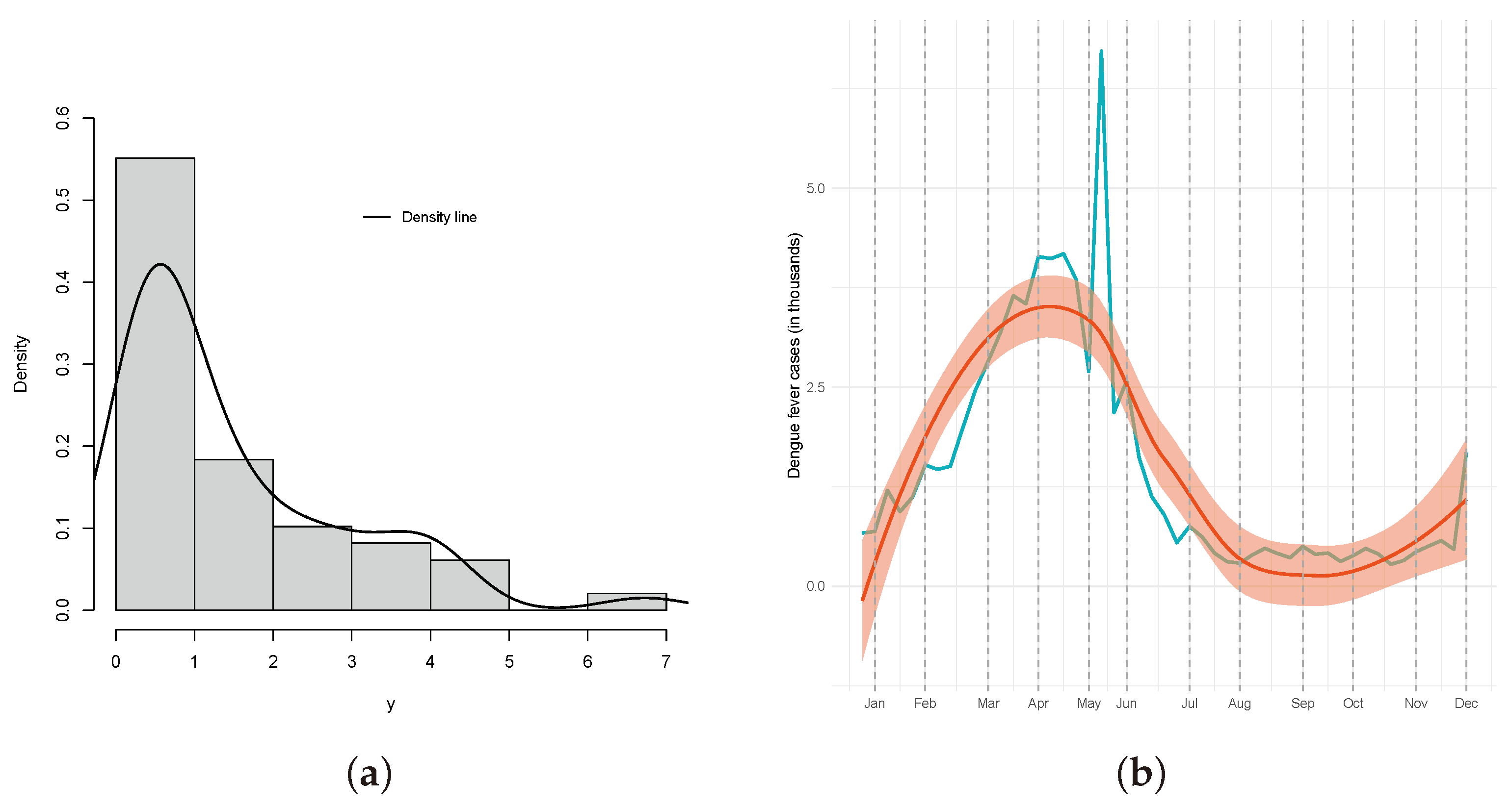
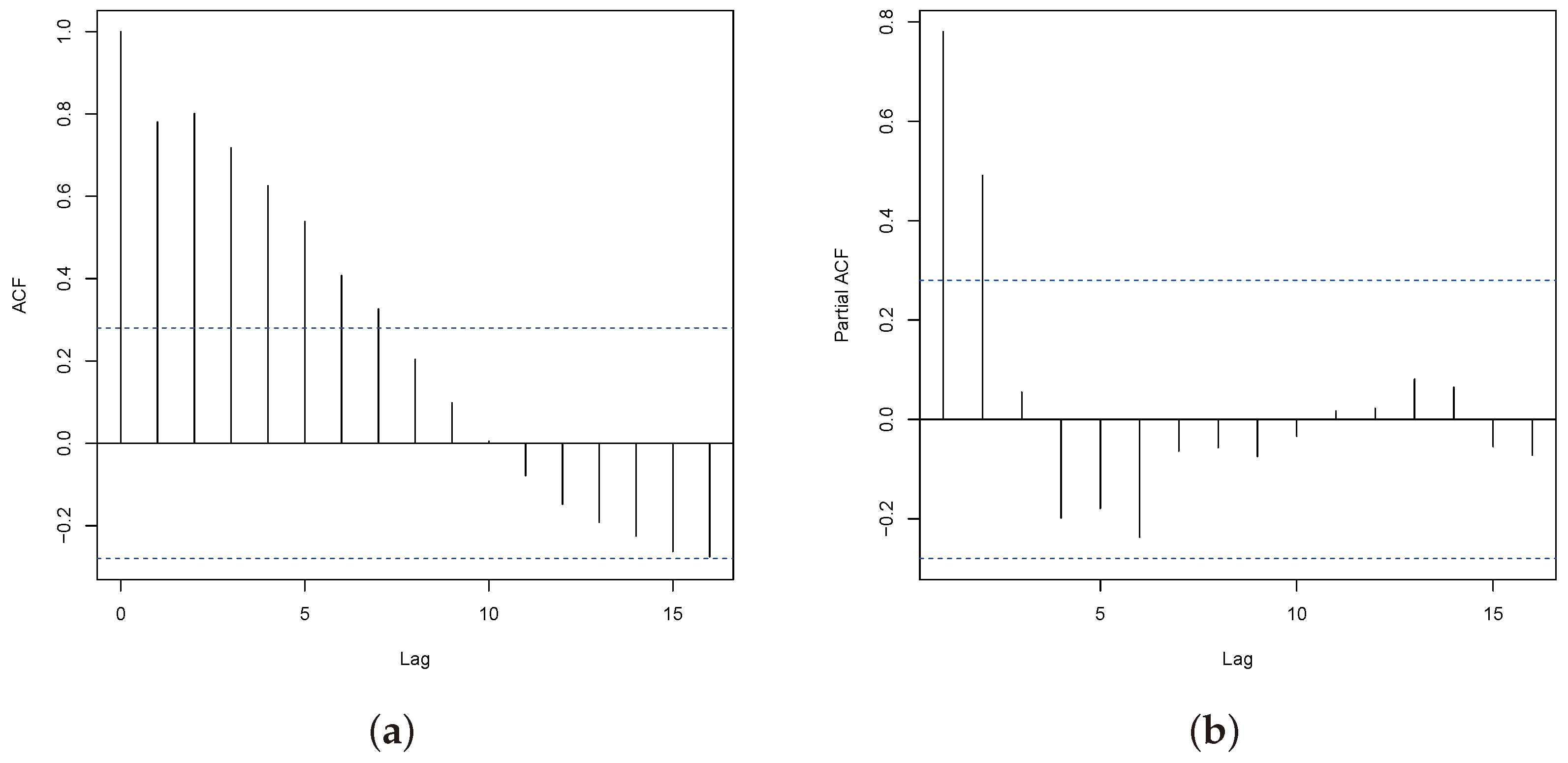
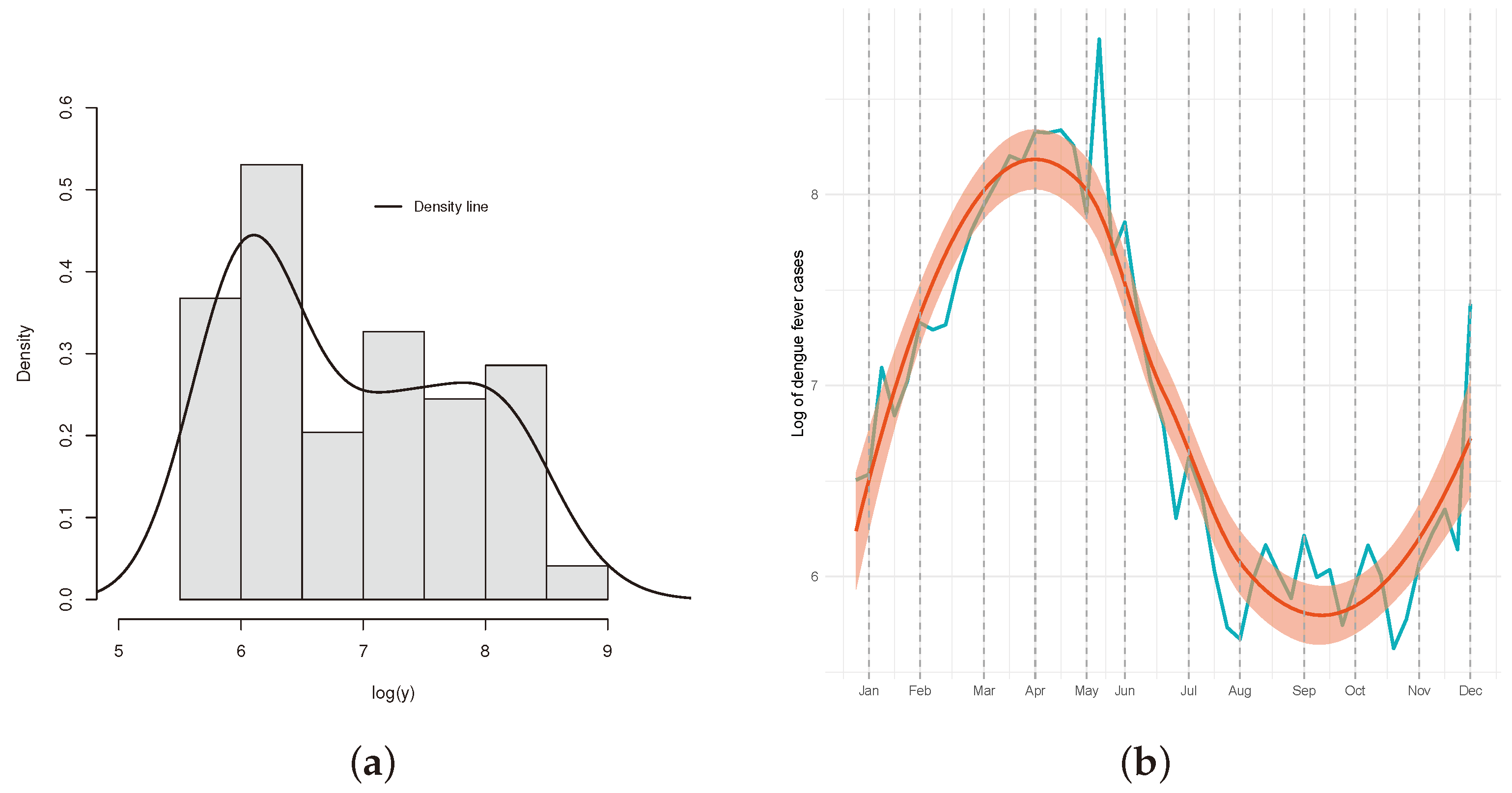
4.1. Descriptive of the Data

The data set was extracted from the Health Problem and Notification Information System (SINAN) (https://datasus.saude.gov.br/acesso-a-informacao/doencas-e-agravos-de-notificacao-de-2007-em-diante-sinan/, accessed on 2 July 2024). SINAN is a repository of patient notifications including a wide range of diseases, injuries and public health incidents listed as nationally mandatory for reporting. Notably, this includes more than 40 diseases (dengue fever, chikungunya fever, pandemic influenza, etc.). The data comprise of notifications related to dengue fever cases reported within the Federal District, Brazil, spanning all 49 epidemiological weeks (observations) throughout the year 2022: 689, 1205, 938, 1121, 1523, 1469, 1508, 1999, 2468, 2827, 3196, 3651, 3550, 4142, 4118, 4178, 3853, 2700, 6726, 2183, 2581, 1616, 1126, 898, 548, 752, 622, 415, 309, 291, 396, 476, 411, 360, 500, 402, 418, 313, 385, 475, 406, 277, 323, 433, 505, 574, 465, 1.682.

The focus of the study is on the variables below:

• $y_i$: total dengue fever cases of a epidemiological week (DG) (response variable);
• $m_{ij}$: month (levels: 0—January to 11—December). Thus, for $i=1,\dots ,49$ and $j=0,\dots ,11$, dummy variables.

The proposed model provides both advantages and disadvantages compared counting models. The exponential distribution used as a baseline has several important characteristics, including applicability in some epidemiological contexts, memorylessness, a good fit featuring heavy tails, flexibility and a simple density function form. Several concerns may arise, such as a lack of flexibility for trend modeling, violations of the independence assumption, and limitations with inflated zero data. Nonetheless, the model captures the significance of the exploratory variables as well as extreme events involving dengue fever patients in the temporal scenario.

Table 6. Descriptive statistics of dengue fever cases data.

Variable	Min.	Max.	Mean	Median	SD	Skewness	Kurtosis
DG	277	6726	1483	752	1445.35	1.509	4.998

presents descriptive statistics. The number of dengue fever cases varied from very low (277) to high (6726). The standard deviation of 1445.35 indicates increased variability in dengue fever cases over time. The distribution is skewed to the right (1.509), suggesting that there are more extreme values at the higher end of the scale, and the kurtosis indicates heavier tails (4.998).

Figure 8 shows the histogram and time series of the data. Figure 8a indicates heavy tail behavior, consistent with extreme event data. Figure 8b shows anomalous activity between May and June. This represents the highest number of cases since 1998, (https://www.saude.df.gov.br/informes-dengue-chikungunya-zika-febre-amarela, accessed on 2 July 2024), demonstrating the atypical behavior of the observations, which deviate significantly from the historical average, indicating an unusual outbreak, or, in epidemiology, an extreme event of dengue fever that can have an impact on both the health system and the economy. In addition, the plot shows an increase in tendency between February and June, when the disease is most likely to develop in the Federal District and a decrease in tendency between July and December, which is the drought period.

Despite being a continental country with varying disease patterns, Brazil’s Midwest region has the highest incidence of dengue fever, as reported by the Arbovirus Monitoring Panel of the Ministry of Health (https://www.gov.br/saude/pt-br/assuntos/saude-de-a-a-z/a/aedes-aegypti/monitoramento-das-arboviroses, accessed on 2 July 2024). This is the region where the study data were collected.

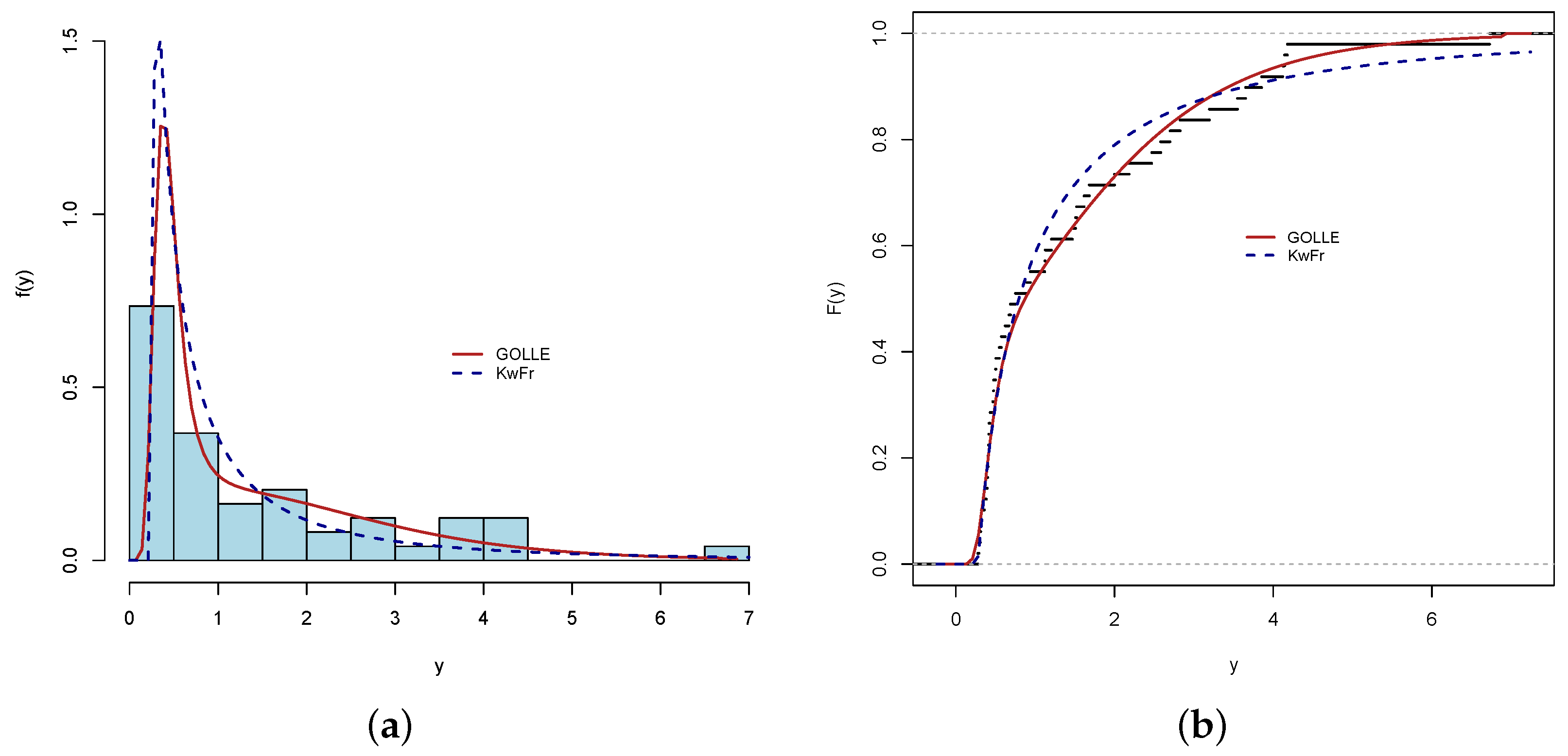
4.2. Findings from GOLLE Distribution

The analysis of time series data requires a detailed inspection, which includes identifying relationships between the observations. Failure to account for these associations may result in an inadequate model that neglects temporal dependence, potentially leading to incorrect forecasts and interpretations. To identify serial correlation, it is essential to analyze the autocorrelation function (ACF) and partial autocorrelation function (PACF) plots. Figure 9 shows the ACF and PACF for an autoregressive integrated moving average (ARIMA) model with one lag in the differenced series, specifically, ARIMA(1,1,0).

Although the dataset shows a correlation, indicating a dependency between variables, the model can still be used if this assumption is relaxed, especially given the small sample size and the implementation of diagnostic and residual analyses.

Table 7. Findings from the fitted models of dengue fever cases data.

Model	Parameters				${\mathbf{W}}^{*}$	${\mathbf{A}}^{*}$	KS
GOLLE † ($\mathit{\alpha },\mathit{\theta },\mathit{\lambda }$)	0.154	76.500	5.402		0.060	0.400	0.077
	(0.018)	(0.019)	(0.003)				(0.914)
OLLE($\alpha ,\lambda$)	1.180	1	0.634		0.318	1.929	0.160
	(0.142)	(-)	(0.086)				(0.145)
EE($\theta ,\lambda$)	1	1.391	0.830		0.313	1.898	0.175
	(-)	(0.284)	(0.147)				(0.088)
E($\lambda$)	1	1	0.674		0.316	1.913	0.170
	(-)	(-)	(0.096)				(0.103)
KwFr($\beta ,\gamma ,a,b$)	3.851	51.070	0.172	0.271	0.087	0.559	0.097
	(1.409)	(71.389)	(0.060)	(0.008)			(0.705)
KwE($\beta ,\gamma ,\lambda$)	4.500	0.151	5.402		0.242	1.482	0.205
	(0.005)	(0.022)	(0.003)				(0.028)
GFr($\beta ,a,b$)	0.465	0.777	0.225		0.128	0.830	0.120
	(0.082)	(0.142)	(0.039)				(0.443)
BE($\beta ,\gamma ,\lambda$)	3.027	0.150	5.402		0.253	1.548	0.197
	(1.054)	(0.023)	(0.003)				(0.038)
GE($\beta ,\lambda$)	1.323	0.892			0.317	1.917	0.173
	(0.241)	(0.197)					(0.096)
Fr($a,b$)	1.791	−0.281			0.235	1.449	0.173
	(0.285)	(0.076)					(0.094)

^† Best fit model in bold.

presents the results of the fitted distributions to the data and shows that the GOLLE distribution is the best fit. Figure 10a,b show histograms and plots of estimated densities, as well as empirical cdf estimated ones. The Fréchet distribution is commonly used to model extreme occurrences and these findings suggest that the KwFr distribution (the second-best model) is competitive with the presented model.

Likelihood-ratio (LR) tests were used to compare the GOLLE distribution with its nested models.

Table 8. LR tests of the GOLLE distribution.

Models	Statistic w	p-Value
GOLLE vs. E	29.657	<0.0001
GOLLE vs. EE	27.143	<0.0001
GOLLE vs. OLLE	27.937	<0.0001

shows that adding more parameters significantly influences the accuracy of modeling the existing data.

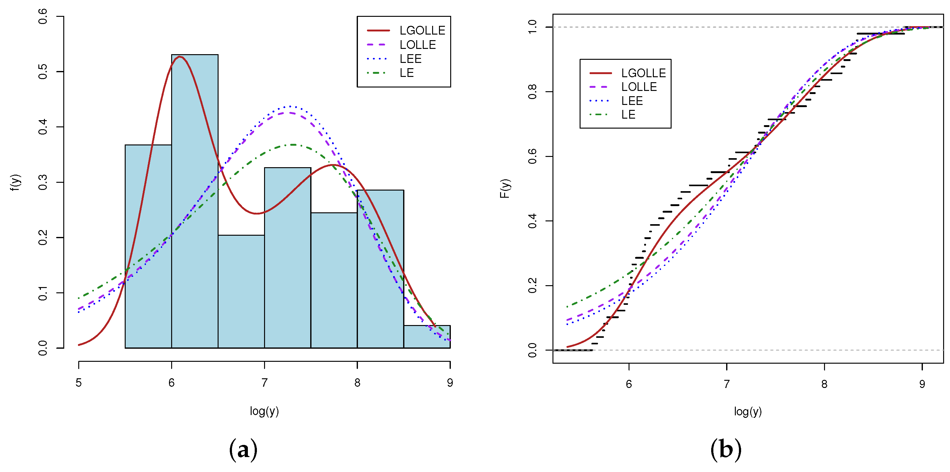
4.3. Findings from LGOLLE Regression Model

To assess the LGOLLE model, Figure 11 displays the ACF and PACF plots for the differenced series ARIMA(0,1,0), which indicates a random walk process. Therefore, the proposed regression model is suitable for the current data set.

A histogram and time series of the log data are displayed in Figure 12. Figure 12a shows a bimodal distribution, with extreme occurrences observed between May and June. Figure 12b illustrates a clear trend over time.

The LGOLLE distribution is the best fit, compared to the nested models log odd log-logistic exponential (LOLLE), log exponentiated exponential (LEE) and log exponential (LE), as demonstrated by

Table 9. Findings from the fitted models of log-dengue fever cases data.

Model	Parameters			${\mathbf{W}}^{*}$	${\mathbf{A}}^{*}$	KS
LGOLLE † ($\mathit{\alpha },\mathit{\theta },\mathit{\mu }$)	0.1517	78.7499	5.2352	0.054	0.3664	0.0862
	(0.0178)	(0.0274)	(0.0034)			(0.8293)
LOLLE($\alpha ,\mu$)	1.1798	1	7.3631	0.3184	1.9289	0.1601
	(0.1423)	(-)	(0.1353)			(0.1453)
LEE($\theta ,\mu$)	1	1.3911	7.0935	0.3132	1.8975	0.1750
	(-)	(0.2839)	(0.1769)			(0.0879)
LE($\mu$)	1	1	7.3019	0.3161	1.9131	0.1704
	(-)	(-)	(0.1429)			(0.1032)

^† Best fit model in bold.

, which displays the results of the fitted nested distributions to the log data. In addition to histograms and the estimated density functions in Figure 13a,b displays the empirical cdf and estimated ones.

LR tests are employed to compare the nested models of the LGOLLE distribution.

Table 10. LR tests of the LGOLLE distribution.

Models	Statistic w	p-Value
LGOLLE vs LE	29.650	<0.0001
LGOLLE vs LEE	27.136	<0.0001
LGOLLE vs LOLLE	27.930	<0.0001

shows that adding extra parameters has a considerable influence on the modeling performance with the given data.

The new LGOLLE regression model for the dengue fever cases data in Federal District, Brazil can be expressed as follows

$$y_i={\mu }_i+z_i,$$

where $z_1,z_2,\dots ,z_{49}$ are independent rv with density function (10) and the systematic structure is defined by

$${\mu }_i={\beta }_0+\sum _{j=1}^{11}{\beta }_j{m}_j.$$

The results (MLEs, SEs, Confidence Intervals (CIs), and p-values) of the fitted LGOLLE regression model are presented in

Table 11. Fitted LGOLLE regression model of dengue fever cases data.

Parameter	Estimate	SE	CI (95%)	p-Value
${\mathit{\beta }}_{\mathbf{1}}$  (Fev)	0.5511	0.1836	(0.1913; 0.9109)	0.0049
${\mathit{\beta }}_{\mathbf{2}}$  (Mar)	1.0827	0.1909	(0.7085; 1.4569)	<0.0001
${\mathit{\beta }}_{\mathbf{3}}$  (Apr)	1.6788	0.1764	(1.3331; 2.0245)	<0.0001
${\mathit{\beta }}_{\mathbf{4}}$  (May)	1.7125	0.1822	(1.3554; 2.0696)	<0.0001
${\mathit{\beta }}_{\mathbf{5}}$  (Jun)	1.4393	0.2262	(0.9960; 1.8826)	<0.0001
${\beta }_6$ (Jul)	0.3091	0.1935	(−0.0702; 0.6884)	<0.1192
${\mathit{\beta }}_{\mathbf{7}}$  (Ago)	−0.5881	0.2006	(−0.9813; −0.1949)	0.0059
${\mathit{\beta }}_{\mathbf{8}}$  (Sep)	−0.4623	0.1723	(−0.8000; −0.1246)	0.0110
${\mathit{\beta }}_{\mathbf{9}}$(Oct)	−0.5778	0.1776	(−0.9259; −0.2297)	0.0025
${\mathit{\beta }}_{\mathbf{10}}$  (Nov)	−0.5749	0.1802	(−0.9281; −0.2217)	0.0030
${\beta }_{11}$ (Dec)	−0.1612	0.1928	(−0.5391; 0.2167)	0.4088
$\alpha$	47.1443	6.4074	(34.5861; 59.7026)	-
$\theta$	0.0751	0.0054	(0.0645; 0.0857)	-

Significant parameters in bold.

. Therefore, using a significance level of $5\%$, the months in the temporal scenario are significant and can be used to model the location.

Figure 14 presents two potentially significant observations based on the LD and GCD measures. It is worth noting that the 20th and 49th observations, correspond to the beginning of June, and the last epidemiological week. The first matches the record (https://www.metropoles.com/distrito-federal/boletim-revela-aumento-dos-casos-de-dengue-em-todas-as-regioes-do-df, accessed on 2 July 2024) of dengue fever cases in the Federal District. The second relates to the end of year vacation/recess period, which results in a backlog of alerts due to a lack of healthcare professionals available to notify cases and input data into the system.

Nonetheless, Figure 15 indicates that the residual deviations behave randomly across the range and remain within the simulated envelope, implying that the observations have minimal impact on the regression model.

4.4. Discussion

The findings indicate that the LGOLLE regression model is suitable for explaining the weekly dengue fever cases in the Federal District. Table 11 presents parameter estimates for the LGOLLE regression model, which becomes (for $i=1,\dots ,49$)

$$\begin{array}{cc}\hfill {\widehat{\mu }}_i& =15.7495+0.5511m_{i1}+1.0827m_{i2}+1.6788m_{i3}+1.7125m_{i4}\hfill \\ \hfill & +1.4393m_{i5}-0.5881m_{i7}-0.4623m_{i8}-0.5778m_{i9}-0.5749m_{i10}.\hfill \end{array}$$

(17)

The following discussion examines the systematic structure, using January as the month of reference.

Interpretations for $\widehat{\mathit{\mu }}$

• Except for the covariates $m_6$ and $m_{11}$, referring to the months of July and December, all other covariates are significant at a $5\%$ level of significance. This indicates that there is a difference in dengue fever cases registered in the Federal District between the other months and January. The months of July and December are probably not significant due to their behavior being similar to the reference month;
• The months of February to June have positive estimates, which is significant, showing an increase in comparison to January. This can be seen in Figure 12b, which shows an extreme event occurring between May and June in the data for that time window;
• The months of August to November have negative values, indicating a decline in dengue fever cases compared to January. During this period, the Federal District experiences a drought, which corroborates the study’s findings (https://portal.inmet.gov.br/uploads/notastecnicas/Estado-do-clima-no-Brasil-em-2022-OFICIAL.pdf, accessed on 2 July 2024).

5. Conclusions

The paper defines the generalized odd log-logistic exponential (GOLLE) distribution (see [12,13]) and introduces a new bimodal regression model based on this distribution, incorporating a location-systematic structure, to investigate weekly dengue fever cases in the Federal District for 2022. The paper reviews some mathematical properties, estimates the parameters using the maximum likelihood method, and evaluates the consistency criterion through Monte Carlo simulations. The consistency of the MLEs for the regression model is assessed using various simulation measures. Additionally, global influence measures and residual analysis are conducted to examine the fit of the new model.

Some important findings are presented. Aside from the months of July and December, the remaining months are significant at the 5% significance level. From February to June, positive estimates are observed, suggesting a positive impact on dengue fever cases during this period. This aligns with the climatological effects that increase cases in these months. Between August and November, a drought occurs, supporting the negative estimates during this period, indicating a negative effect on weekly dengue fever cases.

The epidemiology dataset showed that the novel regression model is more flexible than other nested and well-established models. Therefore, the proposed model enhances the understanding of dengue fever cases in the Federal District and accounts for an extreme event that occurred during the study period. To generalize these findings, further validation across diverse datasets and regions is necessary. Future research should explore the model’s applicability to other diseases or epidemiological settings.

References

1. Joseph, J.; Gillariose, J. A novel discrete Slash family of distributions with application to epidemiology informatics data. Int. J. Data Sci. Anal. 2024, 1–17. [Google Scholar] [CrossRef]
2. Li, Y.; Dou, Q.; Lu, Y.; Xiang, H.; Yu, X.; Liu, S. Effects of ambient temperature and precipitation on the risk of dengue fever: A systematic review and updated meta-analysis. Environ. Res. 2020, 191, 110043. [Google Scholar] [CrossRef]
3. Lim, J.T.; Dickens, B.S.L.; Cook, A.R. Modelling the epidemic extremities of dengue transmissions in Thailand. Epidemics 2020, 33, 100402. [Google Scholar] [CrossRef]
4. Diop, A.; Deme, E.H.; Diop, A. zero-inflated generalized extreme value regression model for binary response data and application in health study. J. Stat. Comput. Simul. 2023, 93, 1–24. [Google Scholar] [CrossRef]
5. Marani, M.; Katul, G.G.; Pan, W.K.; Parolari, A.J. Intensity and frequency of extreme novel epidemics. Proc. Natl. Acad. Sci. USA 2021, 35, e2105482118. [Google Scholar] [CrossRef]
6. Thomas, M.; RootzÉn, H. Real-time prediction of severe influenza epidemics using extreme value statistics. J. R. Stat. Soc. Ser. C Appl. Stat. 2022, 71, 376–394. [Google Scholar] [CrossRef]
7. Lin, H.; Zhang, Z. Extreme co-movements between infectious disease events and crude oil futures prices: From extreme value analysis perspective. Energy Econ. 2022, 110, 106054. [Google Scholar] [CrossRef]
8. Tian, N.; Zheng, J.-X.; Guo, Z.-Y.; Li, L.-H.; Xia, S.; Lv, S.; Zhou, X.-N. Dengue incidence trends and its burden in major endemic regions from 1990 to 2019. Trop. Med. Infect. Dis. 2022, 7, 180. [Google Scholar] [CrossRef]
9. Lun, X.; Wang, Y.; Zhao, C.; Wu, H.; Zhu, C.; Ma, D.; Xu, M.; Wang, J.; Liu, Q.; Xu, L.; et al. Epidemiological characteristics and temporal-spatial analysis of overseas imported dengue fever cases in outbreak provinces of China, 2005–2019. Infect. Dis. Poverty 2022, 11, 12. [Google Scholar] [CrossRef]
10. Sandeep, M.; Padhi, B.K.; Yella, S.S.T.; Sruthi, K.G.; Venkatesan, R.G.; Sasanka, K.S.; Krishna, B.S.; Satapathy, P.; Mohanty, A.; Al-Tawfiq, J.A.; et al. Myocarditis manifestations in dengue cases: A systematic review and meta-analysis. J. Infect. Public Health 2023, 16, 1761–1768. [Google Scholar] [CrossRef]
11. de Oliveira-Júnior, J.F.; Souza, A.; Abreu, M.C.; Nunes, R.S.C.; Nascimento, L.S.; Silva, S.D.; Correia Filho, W.L.F.; Silva, E.B. Modeling of dengue by cluster analysis and probability distribution functions in the state of Alagoas in Brazilian. Braz. Arch. Biol. Technol. 2023, 66, e23220086. [Google Scholar] [CrossRef]
12. Qoshja, A.; Muça, M. A new modified generalized odd log-logistic distribution with three parameters. Math. Theory Model. 2018, 8, 2224–5804. Available online: https://www.researchgate.net/publication/331483356_A_NEW_MODIFIED_GENERALIZED_ODD_LOG-LOGISTIC_DISTRIBUTION_WITH_THREE_PARAMETERS (accessed on 28 June 2024).
13. Afify, A.Z.; Suzuki, A.K.; Zhang, C.; Nassar, M. On three-parameter exponential distribution: Properties, Bayesian and non-Bayesian estimation based on complete and censored samples. Commun. Stat.-Simul. Comput. 2021, 50, 3799–3819. [Google Scholar] [CrossRef]
14. Cordeiro, G.M.; Alizadeh, M.; Ozel, G.; Hosseini, B.; Ortega, E.M.M.; Altun, E. The generalized odd log-logistic family of distributions: Properties, regression models and applications. J. Stat. Comput. Simul. 2017, 87, 908–932. [Google Scholar] [CrossRef]
15. da Costa, N.S.S.; Cordeiro, G.M. A new normal regression with medical applications. Appl. Math. Inf. Sci. 2023, 17, 309–322. [Google Scholar] [CrossRef]
16. da Costa, N.S.S.; do Carmo, M.d.C.S.; Cordeiro, G.M. Analyzing county-level COVID-19 vaccination rates in Texas: A new Lindley regression model. COVID 2023, 3, 1761–1780. [Google Scholar] [CrossRef]
17. Alzaatreh, A.; Lee, C.; Famoye, F. A new method for generating families of continuous distributions. Metron 2013, 71, 63–79. [Google Scholar] [CrossRef]
18. Gleaton, J.U.; Lynch, J.D. Properties of generalized log-logistic families of lifetime distributions. J. Probab. Stat. Sci. 2006, 4, 51–64. Available online: https://www.researchgate.net/publication/283595537_Properties_of_generalized_log-logistic_families_of_lifetime_distributions (accessed on 28 June 2024).
19. Gupta, R.C.; Gupta, R.D. Proportional reversed hazard rate model and its applications. J. Stat. Plan. Inference 2007, 137, 3525–3536. [Google Scholar] [CrossRef]
20. Gupta, R.C.; Gupta, R.D. Exponentiated exponential family: An alternative to gamma and Weibull distributions. Biom. J. J. Math. Methods Biosci. 2001, 43, 117–130. [Google Scholar] [CrossRef]
21. R Core Team. R Core Team: A Language and Environment for Statistical Computing; R Foundation for Statistical Computing: Vienna, Austria, 2024. [Google Scholar]
22. Cox, D.R.; Snell, E.J. A general definition of residuals. J. R. Stat. Soc. Ser. B (Methodol.) 1968, 30, 248–275. [Google Scholar] [CrossRef]
23. Cook, R.D.; Weisberg, S. Residuals and Influence in Regression; Chapman & Hall: London, UK, 1982. [Google Scholar]
24. Ortega, E.M.M.; Paula, G.A.; Bolfarine, H. Deviance residuals in generalized log-gamma regression models with censored observations. J. Stat. Comput. Simul. 2008, 78, 747–764. [Google Scholar] [CrossRef]
25. Silva, G.O.; Ortega, E.M.M.; Paula, G.A. Residuals for log-Burr XII regression models in survival analysis. J. Appl. Stat. 2011, 38, 1435–1445. [Google Scholar] [CrossRef]
26. Atkinson, A.C. Plots, Transformations, and Regression: An Introduction to Graphical Methods of Diagnostic Regression Analysis; Clarendon Press: Oxford, UK, 1987. [Google Scholar] [CrossRef]
27. Mead, M.E.A. A note on Kumaraswamy Fréchet distribution. Australia 2014, 8, 294–300. Available online: http://www.ajbasweb.com/old/ajbas/2014/September/294-300.pdf (accessed on 28 June 2024).
28. Adepoju, K.A.; Chukwu, O.I. Maximum likelihood estimation of the Kumaraswamy exponential distribution with applications. J. Mod. Appl. Stat. Methods 2015, 14, 208–214. [Google Scholar] [CrossRef]
29. Silva, R.; Andrade, T.; Maciel, D.; Campos, R.; Cordeiro, G. A new lifetime model: The gamma extended Frechet distribution. J. Stat. Theory Appl. 2013, 12, 39. [Google Scholar] [CrossRef]
30. Kudriavtsev, A.A. On the representation of gamma-exponential and generalized negative binomial distributions. Inform. Its Appl. 2019, 13, 76–80. [Google Scholar] [CrossRef]
31. Nadarajah, S.; Kotz, S. The beta exponential distribution. Reliab. Eng. Syst. Saf. 2006, 91, 689–697. [Google Scholar] [CrossRef]
32. Fréchet, M. Sur La Loi de Probabilité de L’écart Maximum. Annales de La Societe Polonaise de Mathematique. Available online: https://cir.nii.ac.jp/crid/1572261550191409280 (accessed on 28 June 2024).
33. Marinho, P.R.D.; Silva, R.B.; Bourguignon, M.; Cordeiro, G.M.; Nadarajah, S. AdequacyModel: An R package for probability distributions and general purpose optimization. PLoS ONE 2019, 14, e0221487. [Google Scholar] [CrossRef]
Figure 1. (ac) GOLLE hrf for selected values.
Mathematics 12 03386 g001
Figure 2. GOLLE histogram. (a) GOLLE (0.15, 73, 2.50). (b) GOLLE (0.22, 1.13, 7.50). (c) GOLLE (0.07, 120.13, 3.50).
Mathematics 12 03386 g002
Figure 3. GOLLE distribution. (a) Galton’s skewness. (b) Moors’ kurtosis.
Mathematics 12 03386 g003
Figure 4. Plots of the LGOLLE density function for selected values. (a) For θ = 10.5 and μ = 1 . (b) For α = 0.25 and μ = 2 . (c) For α = 0.17 and θ = 7.42 .
Mathematics 12 03386 g004
Figure 5. (ad) Biases versus sample size from LGOLLE regression model.
Mathematics 12 03386 g005
Figure 6. (ad) MSEs versus sample size from LGOLLE regression model.
Mathematics 12 03386 g006
Figure 7. (ad) ALs versus sample size from LGOLLE regression model.
Mathematics 12 03386 g007
Figure 8. Dengue fever cases data. (a) Histogram and empirical density. (b) Variation across months with trend smoothed line in shadow light red.
Mathematics 12 03386 g008
Figure 9. Dengue fever cases data. (a) ACF. (b) PACF.
Mathematics 12 03386 g009
Figure 10. Fitted models of dengue fever cases data. (a) Histogram and estimated pdfs. (b) Empirical and estimated cdfs.
Mathematics 12 03386 g010
Figure 11. Log-dengue fever cases data. (a) ACF. (b) PACF.
Mathematics 12 03386 g011
Figure 12. Log dengue fever cases data. (a) Histogram and empirical density. (b) Variation across months with trend smoothed line in shadow light red.
Mathematics 12 03386 g012
Figure 13. Fitted models of log-dengue fever cases data. (a) Histogram and estimated pdfs. (b) Empirical and estimated cdfs.
Mathematics 12 03386 g013
Figure 14. The LGOLLE regression model. (a) LD. (b) GCD.
Mathematics 12 03386 g014
Figure 15. The LGOLLE regression model. (a) Deviance residual index. (b) Simulated envelope.
Mathematics 12 03386 g015