Abstract
This work presents a numerical mesh generation method for 3D urban scenes that could be easily converted into any 3D format, different from most implementations which are limited to specific environments in their applicability. The building models have shaped roofs and faces with static colors, combining the buildings with a ground grid. The building generation uses geographic positions and shape names, which can be extracted from OpenStreetMap. Additional steps, like a computer vision method, can be integrated into the generation optionally to improve the quality of the model, although this is highly time-consuming. Its function is to classify unknown roof shapes from satellite images with adequate resolution. The generation can also use custom geographic information. This aspect was tested using information created by procedural processes. The method was validated by results generated for many realistic scenarios with multiple building entities, comparing the results between using computer vision and not. The generated models were attempted to be rendered under Graphics Library Transmission Format and Unity Engine. In future work, a polygon-covering algorithm needs to be completed to process the building footprints more effectively, and a solution is required for the missing height values in OpenStreetMap.
Keywords:
3D city model; spatial model; static 3D reconstruction; building information modeling; OpenStreetMap; computer vision; Google Maps MSC:
51-08; 68U05; 68U07; 68T45
1. Introduction
Research to achieve 3D reconstruction has always been a challenging goal, as it represents a scientific problem and a core technology across various fields, making the accurate and efficient generation of 3D models fundamentally important to a wide range of practical applications.
Most methodologies for mesh generation were designed for a specific file format or engine environment. A method for mesh creation that is not restricted to this specification needs to be polyhedral. This means creation using the fundamental principles of 3D meshes, obtaining the position of each vertex and its interconnections enclosed in polygons.
This work presents a method for the polyhedral generation of 3D urban models, combining buildings and the terrain, with explanation of some specific applications. The initial focus of the proposed method was the simulation of radio propagation in 3D space [1,2], usable for different 3D application programming interfaces (API).
To obtain the 3D models, city modeling and reconstruction involve various techniques. City modeling can be performed using open-source information, of which there are various mature dataset types. Much Geographic Information System (GIS) data can be used directly, such as building footprints in OpenStreetMap definitions [3,4,5], various datasets provided by the registration authority [6], and databases containing building models or photogrammetry data [7]. Others can be processed to obtain usable information, like the building heights from the difference between the Digital Surface Model (DSM) and the Digital Terrain Model (DTM) [3,4,8,9]. The DTM can also be used to create the ground grid model itself [6]. There is also research concerning modeling more entities in the urban ecosystem, like urban trees as in the work of Rantanen et al. [10].
Another technique is 3D inverse rendering, involving extracting a 3D model from a 2D image. It is used in the work of Knodt et al., where modeling is based on the light transport between scene surfaces, supported by neural network techniques [11]. Another example is the work of Garifullin et al. [12], which uses a genetic algorithm comparing the background shadow of the generated model with the input 2D image, creating colorless results.
Procedural modeling can create scenes using defined rules and functions. Biancardo et al. created a procedural tool specified for road design [13]. Alomía et al. performed a case study on integrating procedurally generated road network models with existing GIS data in a model [4]. Bulbul proposed a procedural modeling method to design a small town, providing a terrain grid and the weight values for certain high-level semantic principles of town planning [14].
Some generations have been specified for historical buildings and cultural heritage sites. The work of Ma involved creating models for these buildings to simulate them in virtual reality [7]. Tytarenko et al. carried out a case study to reconstruct a fortress that no longer exists, overlapping modern information and ancient information from old cartographic sources [15].
There are also particular ways of modeling. The work of Kim et al. [16] integrates multiple techniques to generate a model for any city using a single street photo, estimating which is the city with the taken photo to create its model. La Russa et al. performed a modeling study [17] with very high complexity and precision, using predominantly terrestrial sensor scanning to obtain the point cloud, and then using Artificial Intelligence (AI) and a visual programming language to obtain a parametric City Information Model (CIM).
Research conducted on computer vision for building analysis includes approaches to classification tasks and machine learning processing [18]. These approaches face challenges in terms of data availability, reproducibility, and comparability.
For classification and detection tasks, Shahzad et al. performed experiments with Computer Vision (CV) to detect and spotlight buildings in high-solution radar images [19]. Zhou et al. worked to create a digital twin from a single-view image stream, using CV for labeled object detection for estimated indoor building modeling [20].
Some CV tasks have been performed to create building models directly. García-Gago et al. presented a method of 3D modeling from multiple classic photos taken manually by digital cameras [21]. Faltermeier et al. used CV to classify the geographic orientation of roof faces from aerial imagery, and adapted the coordinates to these orientations in the model to generate [22].
Other CV techniques can be used for building analysis even though they are not specific. Ruiz de Oña et al. published a tool for points matching between photos taken from different angles [23]. There is a neural network called the Neural Radiant Field (NeRF) for 3D inverse rendering, which can learn the scenes from images and poses only [24].
Modeling and simulation of ray tracing are commonly applied in urban scenes for radio-propagation analysis, requiring a presented city model. The tool of Egea-Lopez et al. uses a scene generation approach whose functionality lies in its integration with the Unity game engine [5]. The work of Eller et al. simulates radio-propagation on an existing city model that combines terrain and building data [25]. Gong et al. created a method for antenna positioning optimization using radio-propagation simulation [26].
The ray-tracing process may use alternative techniques. Alwajeeh et al. created a ray-tracing channel model for 3D smart cities using 2D approaches, with a standard deviation of 8.66 dB [27]. Choi et al. presented a simulator using an inverse algorithm, including objects in movement, such as vehicles, within a smart city scene [28]. Hansson et al. used equation-based intersections for curved surfaces instead of standard triangulated models [29].
Van Wezel et al. presented an interactive educational tool for learning ray tracing and its components [30]. This tool also includes advanced concepts, such as soft shadows, with gradient luminosity. This occurs when the light source cast on the objects is an area instead of a point.
Hypothesis
As mentioned initially, the generated models are desired to be usable in different 3D renders and engines, with definitions that can be easily converted, instead of in some specific environments as in much previous research, such as the Drawing Exchange Format [9], CityEngine [16], Unreal Engine [6], or the Unity Engine [5,7,10,14].
This generation requires parametric information about the objects. The simplest way to obtain the needed information is to extract it from existing data mining tools and open datasets. This paper uses the Shuttle Radar Topography Mission (SRTM) dataset [31] and OpenStreetMap (OSM) [32]. However, OSM rarely provides all the parameters needed, and some complementary methods need to be provided to fill or edit them manually to fix them. The technique can also reconstruct unreal scenes, providing the 2D footprints and parameters in a suitable format.
This research will progressively consider the following:
- An approach to creating a universal method to generate building models over a ground grid.
- The appropriateness of creating real urban environments, using SRTM and OSM information as input to the method.
- The effectiveness of integrating computer vision to the method to improve the quality of the model generated.
- The usability of the method for environments with procedurally generated or user custom definitions.
The subsequent sections of this paper are organized as follows: Section 2 describes the method to generate the 3D scene and its integrations. Section 3 presents the application of the technique and its results. Section 4 discusses the achievements of this work with regard to the hypothesis. Finally, Section 5 presents some in-progress ideas to be completed in the future.
2. Materials and Methods
The method described in this paper generates the contained objects based on a ground grid. The objects are represented by 2D footprints and decorated with appropriate parameters. The output volumes are detailed in vertices, triangle indices, face material, and face colors, to ensure their universal usability for any 3D renderer. The details are obtained using a numerical approach.
As mentioned before, extracting the required information from the SRTM dataset [31] and OSM [32] is the simplest way to use the method, requiring only a bounding box of latitude and longitude to create a scene referred to in the real world. The SRTM dataset chosen is a DTM with a grid dimension of 90 m and a height precision of 1 m.
When using existing datasets with information on scenes in the real world, the missing information can be filled in from different sources. In this paper, satellite images were used to classify the roof shape of the buildings when OSM did not provide them.
Custom scenes can also be generated if information similar to the previous sources is provided.
2.1. Reconstruction Core
The main generation process does not need specific hardware and is cost-effective. It allows the integration of additional resources to improve the result quality, adjusting the object decorating parameters. The overall efficiency mainly depends on the integrations.
2.1.1. Ground Grid
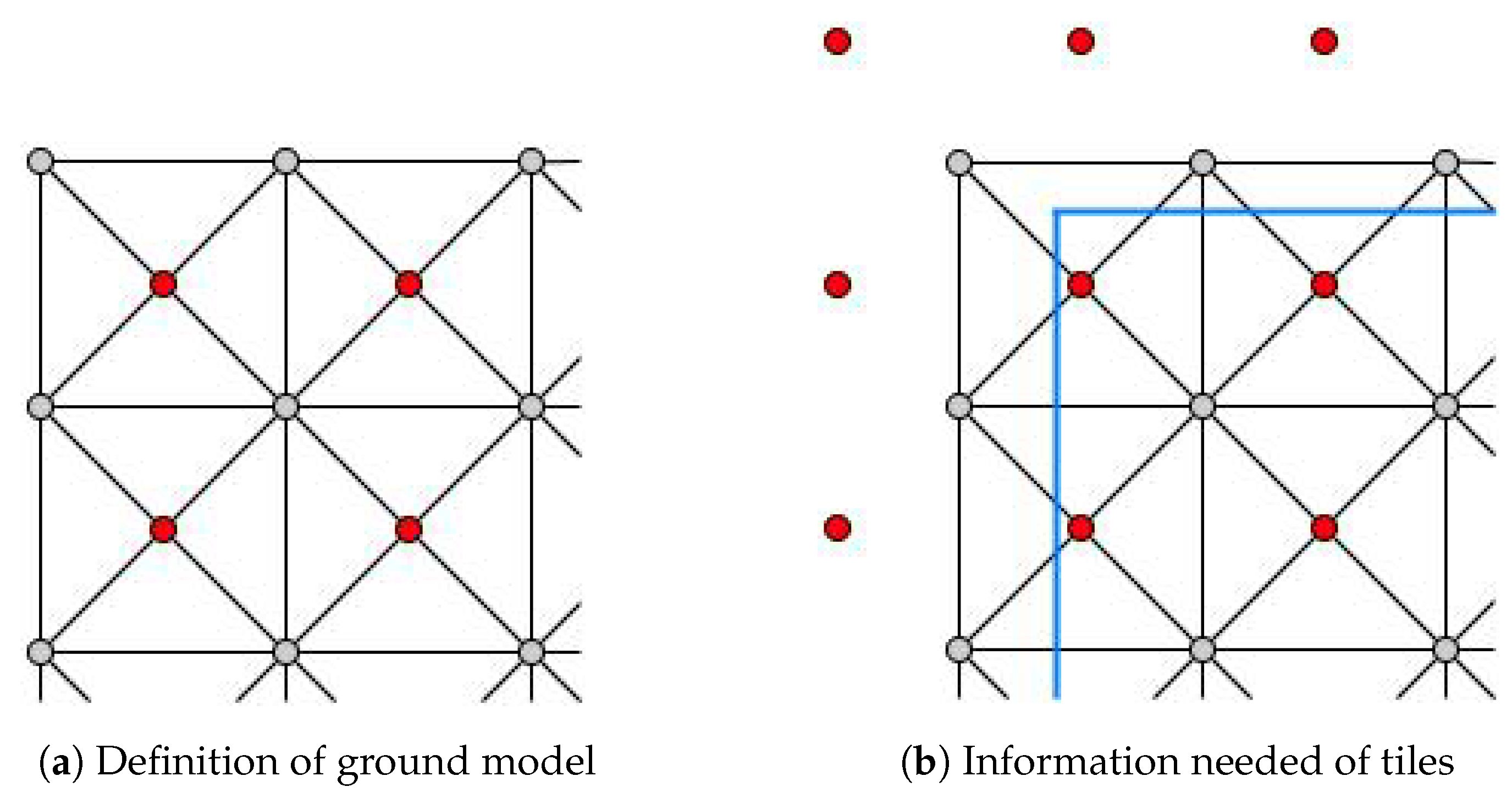
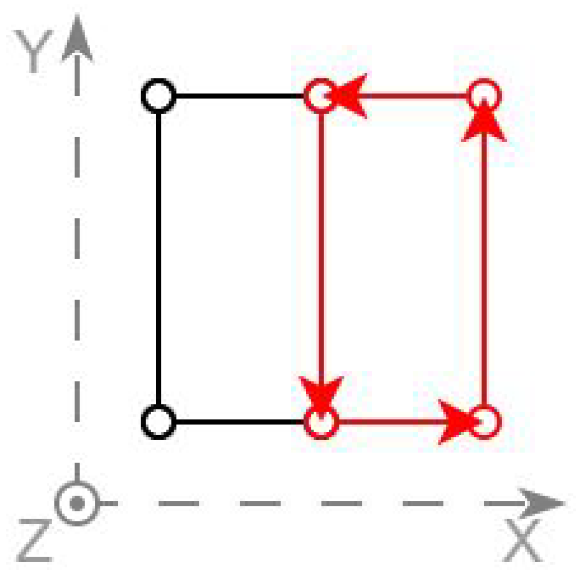
The ground grid is defined by 2D tiles with an elevation value, represented by the center points of each tile. The modeling idea is to maintain each tile as a rectangle from the top view, as shown in Figure 1a. The red points are the tile centers, and the grey points are the tile corners. To create an accurate 3D model, each tile is decomposed into four triangles by its diagonals.
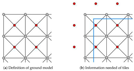
Figure 1.
Tiles to consider to create the ground grid model.
The average value of the surrounding tiles yields the elevation for the corners. Due to this aspect, additional tiles should be provided to obtain the corner elevations at the area perimeter. Regarding Figure 1b, with the blue lines as the border of the required area, the generation needs all the intersected tiles and surrounding ones.
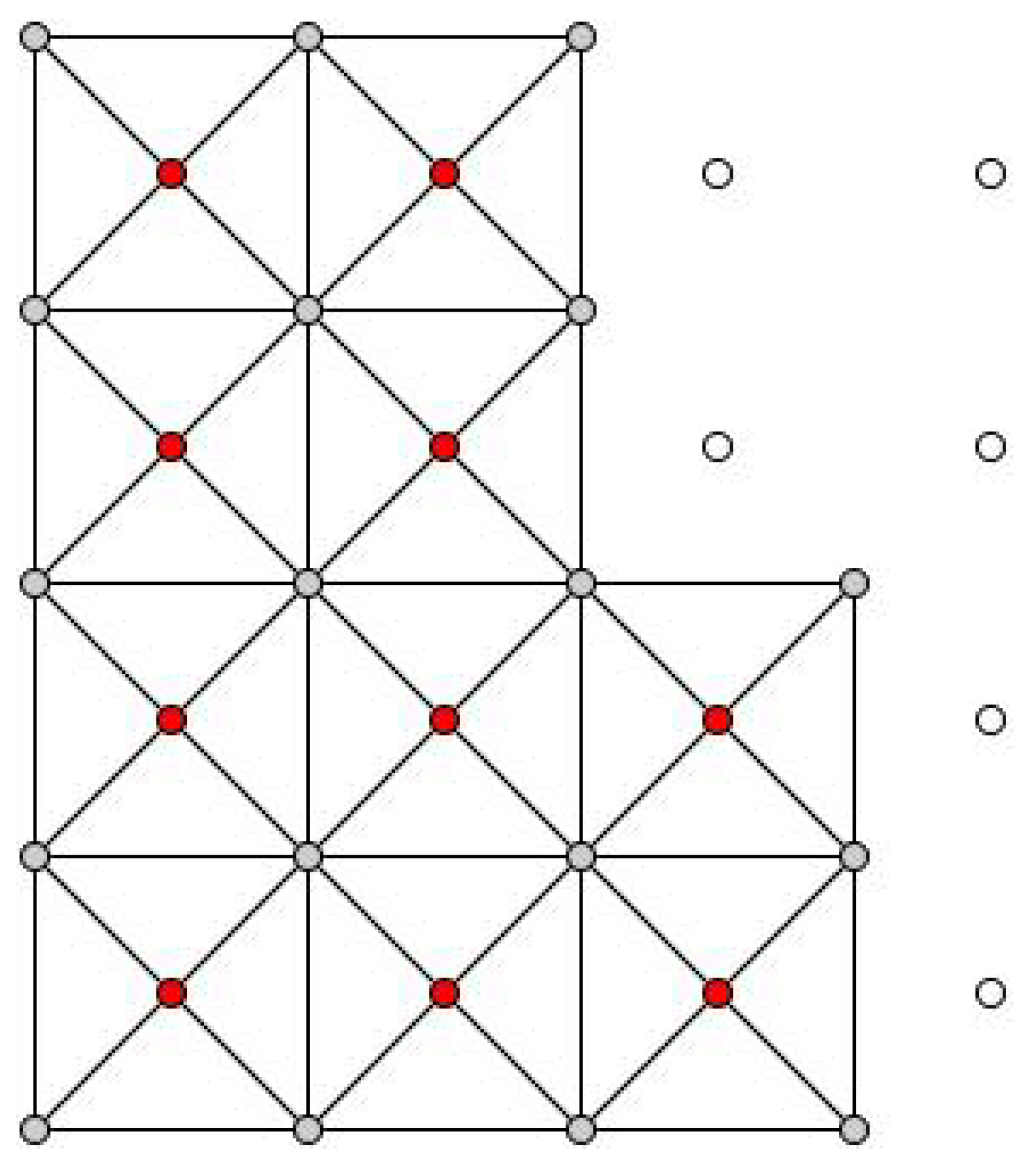
In addition, SRTM information contains empty tiles. The tile values are the ground elevation over the sea level, so the tiles in the water have no value. The generated coastal areas may include some empty spaces, as shown in Figure 2. These tiles will not be incorporated into the 3D model.

Figure 2.
Empty ground tiles (white points for tiles which have no value).
2.1.2. Objects Elevating Rule
The ground model is also used as the elevation reference for any other objects in the scene. With the generated 3D vertices for the ground, the elevation of any middle coordinate can be obtained, as long as the ground is not empty at that point, and none of the objects are placed in an empty position.
According to the coordinate precision of the ground tiles (1/1200 for this paper), a scaled 2D reference is needed, obtained by dividing the coordinate precision. Each unit in the reference values corresponds to an index in the referenced dimension. The coordinate is on the boundary between two tiles when the reference value has no decimals in one dimension. The coordinate is a tile corner when both dimensions have an integer reference value.
To determine the elevation of a point, the coordinates are first scaled according to the precision of the ground tiles. The integer portion of the scaled values in both dimensions will identify the specific tile to which the point belongs. Next, the decimal portion of the reference values is used to determine the corresponding triangle within the tile, based on the diagonals, as depicted in Figure 3.
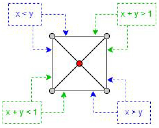
Figure 3.
Tile triangles and equation of diagonals: how to divide each tile with a valid value to infer which triangle belongs to a point.
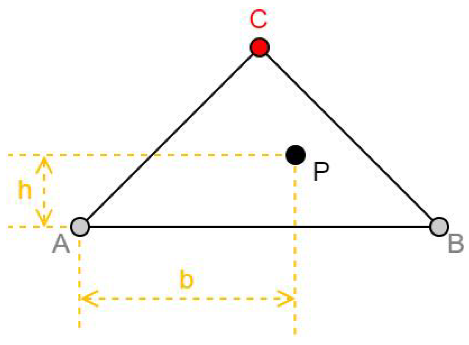
Finally, labeling the elements as in Figure 4, the exact value of a point P in the belonging triangle is obtained using Equation (1).
where C is the center of the tile, A and B are corresponding corners of the tile triangle, and the subscript z means the elevation value of the corresponding point. The value b is the distance from A to the normal projection of P on the segment, with a domain of . Analogously, h is the distance from A to the projection of P on a segment perpendicular , with a domain of . Both b and h are derived from the decimal part of the reference value, and each must be equal to the corresponding decimal part or be its difference from 1.

Figure 4.
Elements labeling in the triangle: to obtain the exact elevation inside a tile triangle.
2.1.3. OSM Buildings
In this paper, the most important goal of the generation is detailed for building models, making requests for OSM entities with the tag “building” or tag “building:part”.
The following information from OSM is used to generate a 3D model for each building entity:
- 2D footprints
- Roof shape and possible parameters
- Total height
- Roof height (when the roof shape is not flat, total height ignoring the body)
- Bottom height (when it does not start from the ground level)
- Colors and materials for body and roof
OSM provides the footprint coordinates in latitude and longitude, and the heights in meters. To create the 3D models, the distance unit must be unified, and a conversion of the coordinates to the Mercator system is required, which represents the coordinates in meters.
For all the generated 3D volumes, their top faces should represent the roof shape, and their floor face must be under the ground unless it has a positive bottom height value. A single flat face can represent the bottom face.
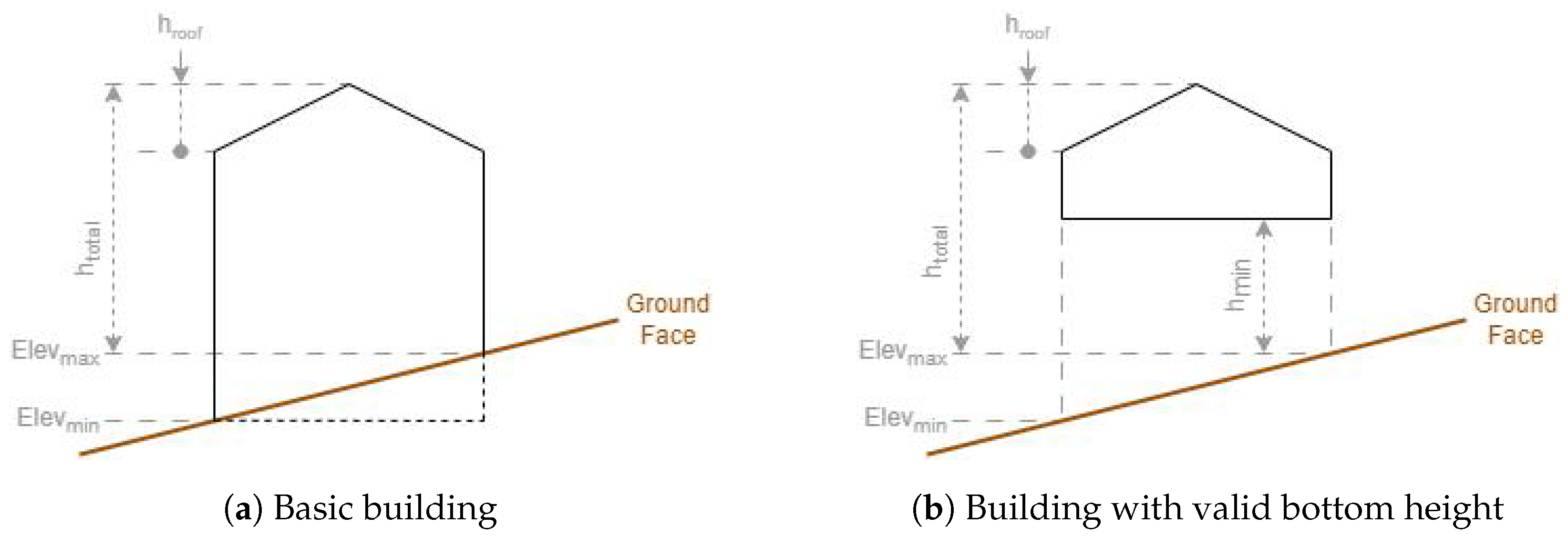
Using the rule defined in Section 2.1.2, an elevation value will be obtained for each point at the outer ring of the building entity footprint. The minimum and maximum of the footprint elevations will be combined with the building height values, as illustrated in Figure 5, to obtain the Z coordinate of the vertices. is the total height, is the roof height, is the bottom height, and and are the extremes of elevations of the footprint coordinates on the ground.
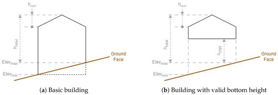
Figure 5.
Theoretical side view of a building model: the ground elevations are from points in the building footprint area.
The rest of the faces are related to the roof shape, where the top view corresponds with the footprint coordinates.
Most of the buildings in the world have a rectangular footprint shape. The definition of the roof shapes is also described using volumes with a rectangular bottom face; therefore, the basis of coordinate processing used in this method is also rectangular.
Considering this basis, the model generation is quite simple and predictable for building entities whose footprint is a simple rectangle, but entities with different footprint shapes need to be adapted to the basis.
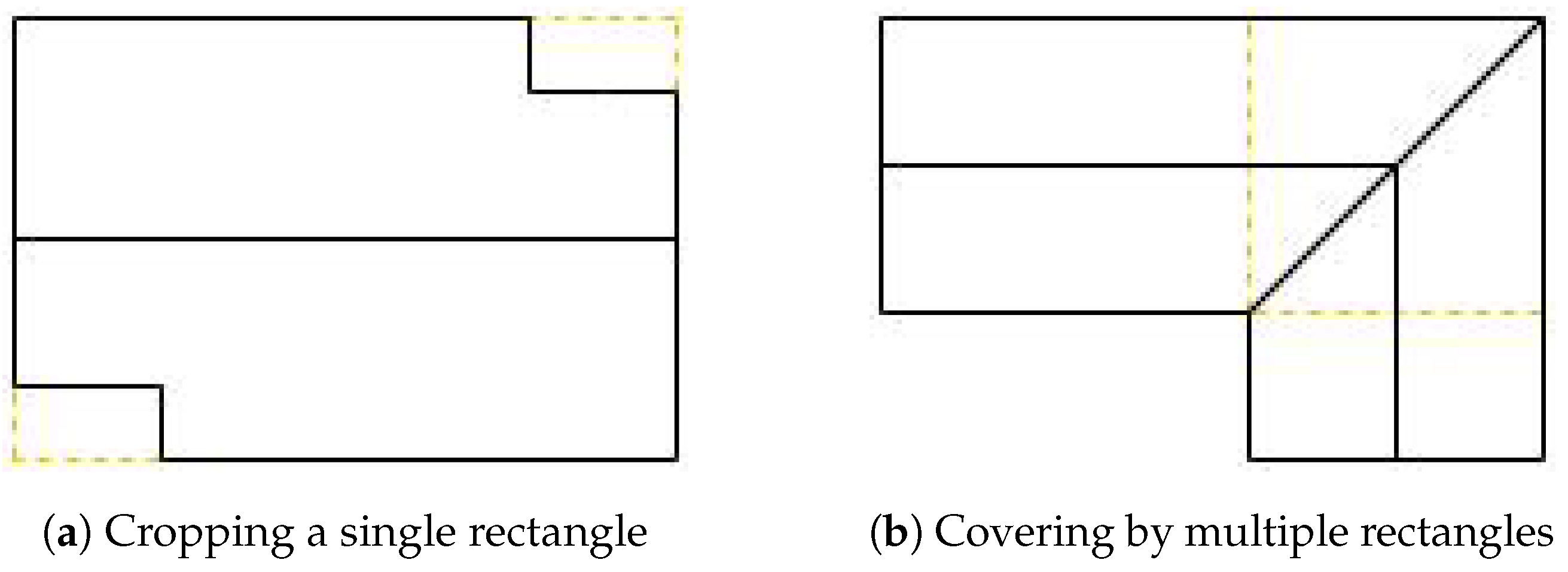
Figure 6 shows two different ways to do this. The first way is to find the smaller rectangle that contains the coordinates and have the redundant parts cropped in the generated 3D model. The second way is to apply a polygon-covering algorithm, filling the coordinates with a minimum number of rectangles.
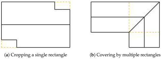
Figure 6.
Ways to adapt footprint coordinates to the rectangular basis.
This method uses the first way, to find the smallest containing rectangle, calling its corresponding 3D model the Virtual Rectangle Roof. Taking this virtual roof as a reference, all the existing points on the roof of the generated model have the same height as the corresponding position on it (it can be a point for a virtual face, not necessarily a vertex).
Alternative Coordinate System
Certain processing is required before starting the building model reconstruction, with the calculation in 2D space, independently for each building entity.
An alternative coordinate system is used to simplify the task, with corresponding translation equations, to obtain the coordinates for the containing rectangle and many other coordinates listed in this section.
The idea is to find two alternative coordinates according to the facing direction of the sides, having all sides parallel to one of them. There are many challenges to comprehensively creating this method:
- The rectangular shape of the footprint coordinates is conceptual, the turning angles are not perfectly perpendicular, and the opposite sides are not perfectly parallel.
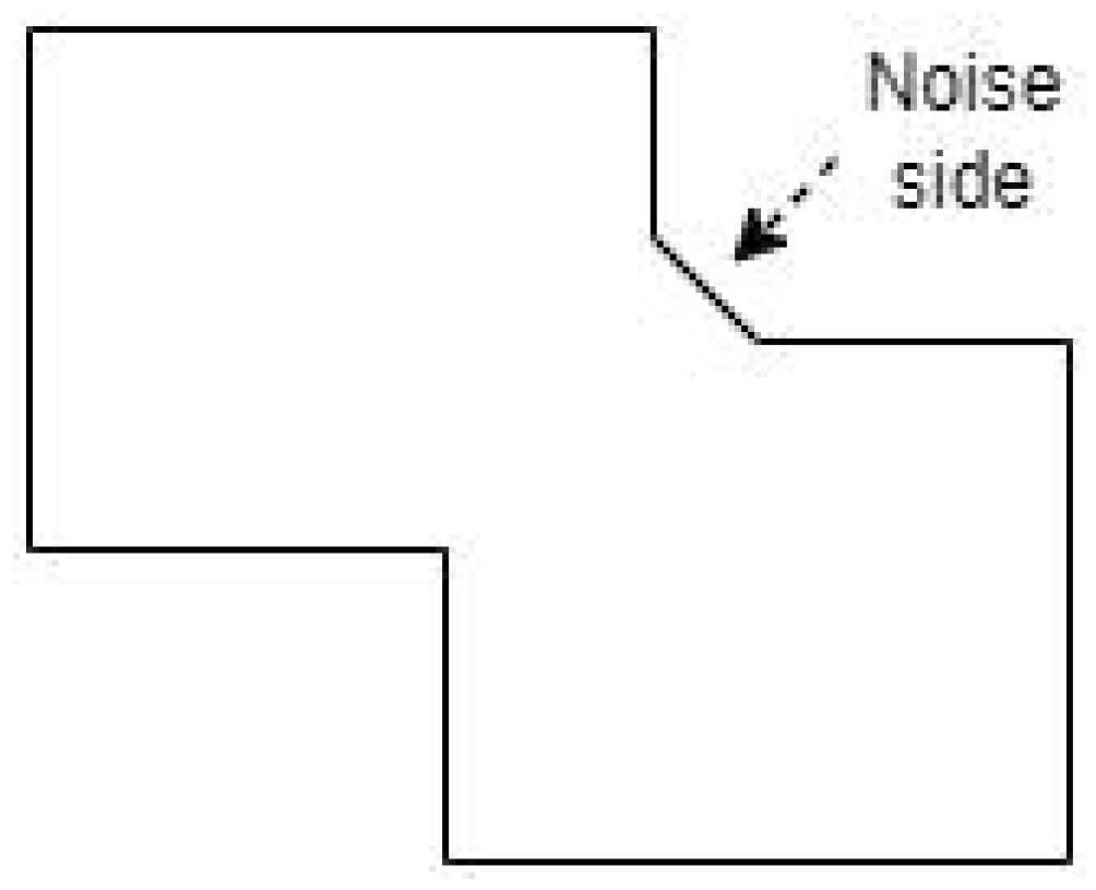
- Some noise angles may be present in the coordinates for sides that are not conceptually perpendicular to adjacent sides (like Figure 7), as well as for circular sections of the building.
 Figure 7. Example of noise side that obtains incorrect direction for the alternative coordinate.
 - The sides of some shapes can not correspond with only two sides having facing directions, such as hexagonal or completely circular coordinates.
The proposed approach finds the mandatory side directions to maintain the functionality in any case.
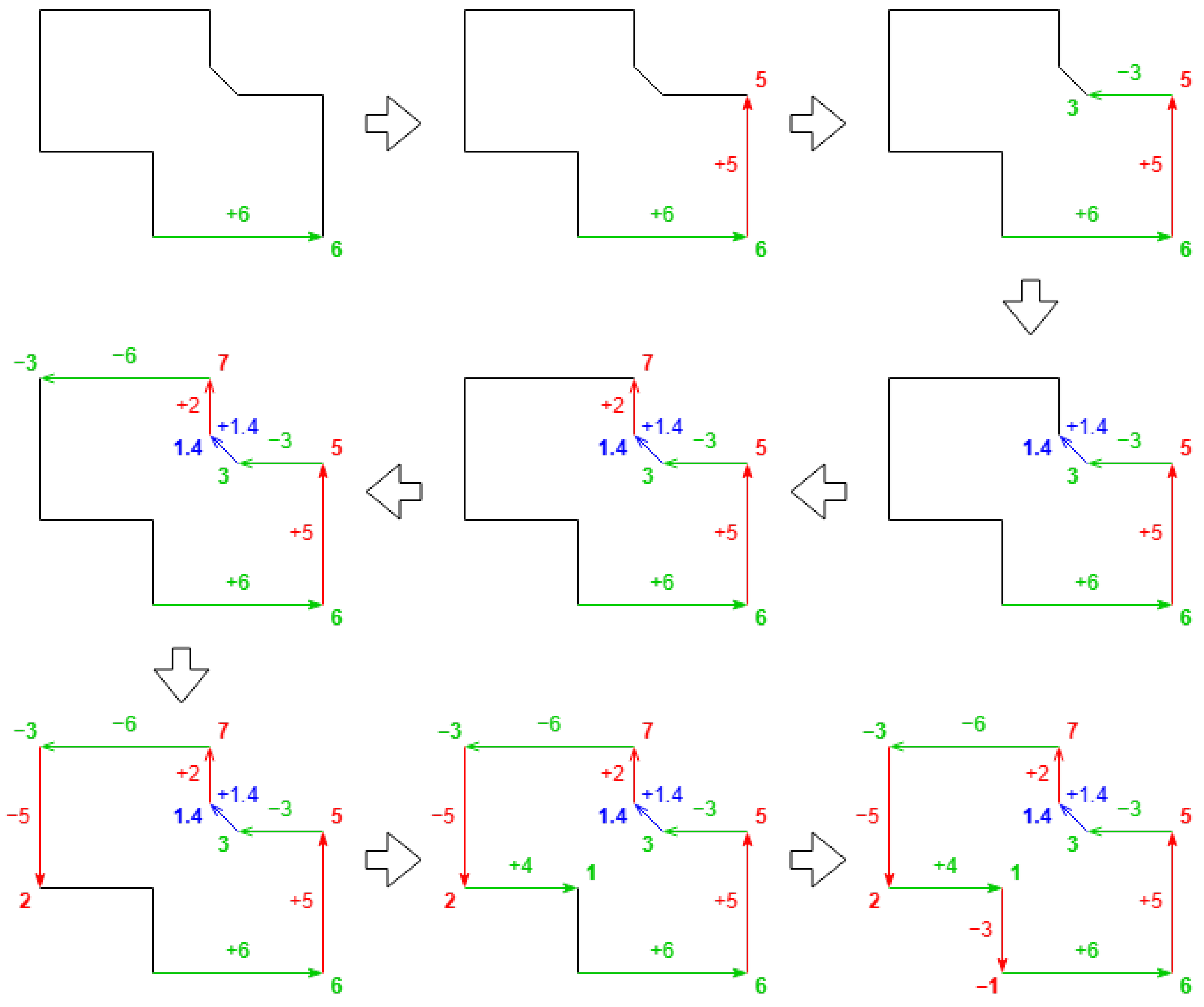
First, the outer sides of the footprint coordinates are walked through to obtain accumulation values of the side lengths. In the middle steps, the sides are grouped by their facing direction. The module length value is added when they have the same direction and is subtracted when they have opposite directions. Knowing the sides may not be perfectly parallel, the dot product of their unit vectors is considered to validate the parallelism of the two sides. When the value exceeds , the sides are determined to have the same direction. If the value is below , the sides are considered to have the opposite direction. In all other cases, the sides will not be grouped.
For each group, the range of the middle accumulation values will be considered the provisional side length, and the direction of the two groups with maximum range will be used to create the alternative coordinates. This process guarantees only the length order, not the real length value.
An example is shown in Figure 8. The range of the green direction is , with provisional length 9. The range of the red direction is , with provisional length 8. There are no valid ranges for the blue direction, having only one value. This first step concludes that the green direction is the longest, and the red direction is the second, which is correct.
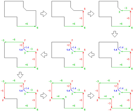
Figure 8.
Example step-by-step walk through of the outer sides; each color represents a different direction.
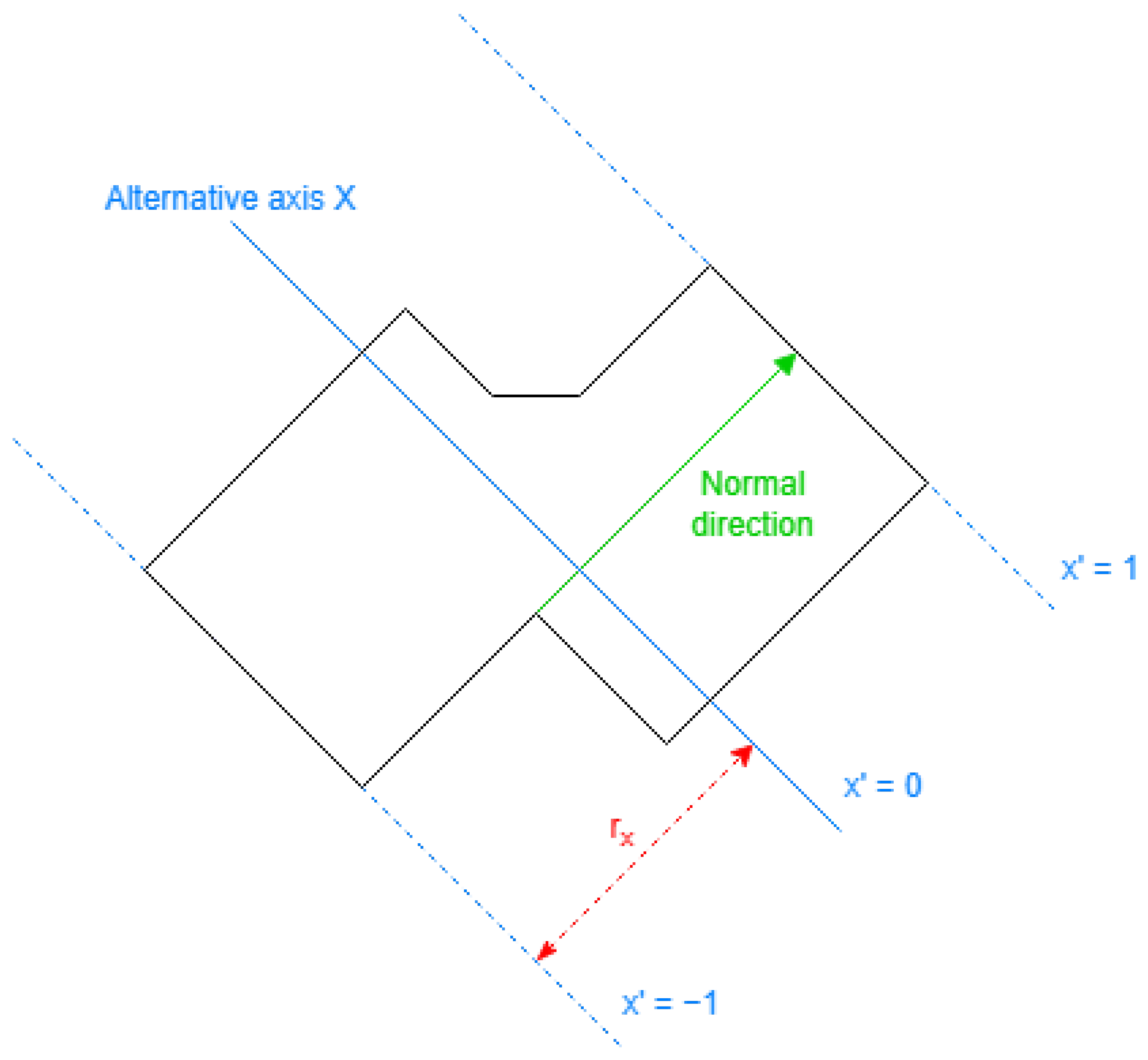
These two directions create the alternative coordinate system, each representing an alternative direction (normal to the alternative axis). An important aspect of the system is distributing all the points in the original coordinate in the range.
The translation equation for each alternative coordinate needs a center parameter and a radio parameter obtained with Equation (3), using the range of values obtained with the positioning Equation (2) for every point in the outer ring.
is the normal vector to the alternative axis obtained previously, for the alternative coordinate for values.
Applying the same for the other alternative coordinate, the final translation equations are as follows (Equation (4)):
is the normal vector for values and for values. An overview for an alternative coordinate is displayed in Figure 9.
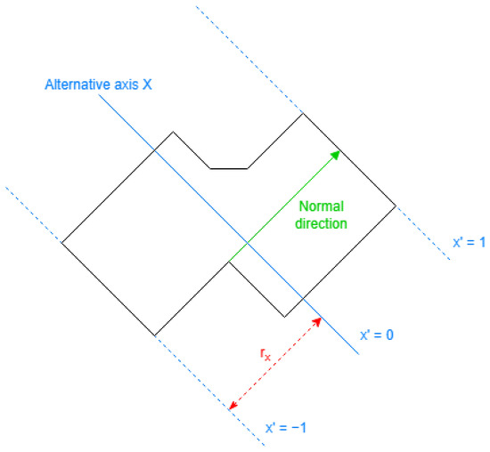
Figure 9.
Alternative coordinate overview: definition of the parameters to obtain those coordinates.
As mentioned previously, the length values obtained in the walking-through step are not guaranteed to be real. For the example in Figure 8, the provisional length is correct in the red direction, but the real length for the blue direction is 10. This can be obtained with the range of values using Equation (2).
The translation can be reversed using both alternative coordinates by solving a simple linear equation system with two unknowns (Equation (5)):
And the point will be defined by values .
Side Segments
Each segment in the 2D footprint results in a body face in the generated model, perpendicular to the ground. Each of these faces shares only one segment with the building floor face, whose XY positions are equal to the segment of footprint coordinates. However, more than one segment can be shared with the building roof faces, depending on the roof shape of the building entity.
The data provided by OSM encompass all entities intersecting the specified area. Regarding building entities partially within the region, their footprint coordinates are truncated at the area’s border, and the resulting segments are derived from these truncated coordinates. The alternative coordinates are derived from the original footprint, before truncation, and are not adjusted to the truncated coordinates.
Considering only the 2D position of these roof segments, the concatenated segment also corresponds with a footprint segment. The opposite is needed to obtain these segments, finding the middle points to divide each segment.
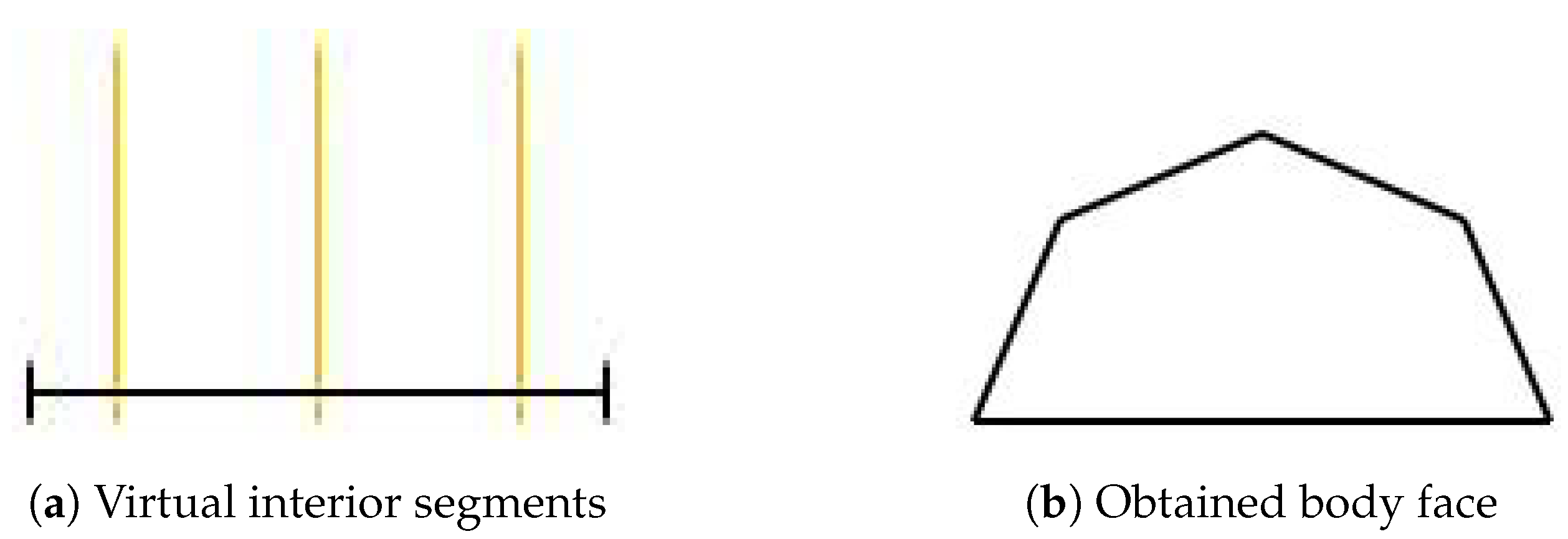
Each roof shape has definitions for interior segments dividing the rectangle. When a footprint side intersects with one of those segments, a dividing point exists for the roof segments. These definitions are positioned in the alternative coordinate, and a reverse translation is needed to check the intersections.
In Figure 10a, where the orange segments are the virtual interior segments, the roof segments will result as Figure 10b.
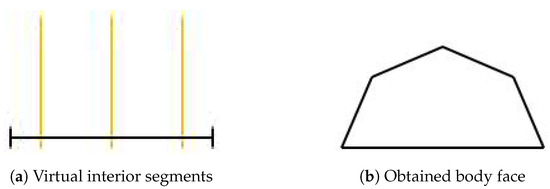
Figure 10.
Example representing a body face, with XY position of the roof segments obtained by the interior segments of the virtual rectangle roof.
Roof Polygons
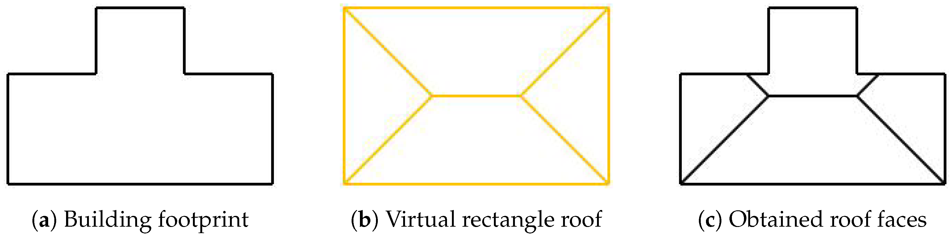
The XY coordinates of the roof faces are the 2D intersection of the building footprint and a face on the virtual rectangle roof. The area border also cuts the faces as the side segments.
The faces on the virtual rectangle roof are defined separately for each roof shape, with the XY positions described in the alternative coordinate system, like the side segments.
For example, a building with the coordinates shown in Figure 11a, whose roof shape corresponds with a virtual rectangle roof like Figure 11b. The obtained real roof faces will be similar to the virtuals, as illustrated by Figure 11c, cropping the concave parts in the building footprint.
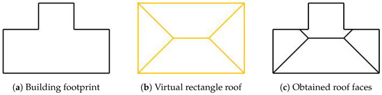
Figure 11.
Representation of 2D coordinates of roof faces: real roof faces obtained by 2D intersections of the footprint with the virtual rectangle roof.
Descending Level Function
In this step, the position of the Z-axis is added to all the vertices on the roof, required by the side faces and the roof faces. With this, an individual model is completed for each building entity.
Each roof shape can be represented by particular functions that consider the positions on the alternative coordinate system, named the Descending Level Function (DLF). These functions obtain the height value of each point on the roof descending the total height value by a portion of the roof height value.
Some roof shapes consider only one alternative coordinate, where the result of the DLF can be used directly to obtain the point height (see Equation (6)).
When both alternative coordinates are considered for a roof shape, define a DLF for each coordinate. The coordinate is always the longest one (), and the results of the point height consider the maximum value of both DLFs, as shown in Equation (7).
The definitions of each roof shape are detailed in Appendix A.
2.1.4. Volumes Union
Finally, the generated volumes of the building entities should be united in 3D space, when their volumes are intersected, eliminating the unnecessary faces between the intersected volumes. This process will reduce the size of the transferred information and computational consumption for diffractions in the ray-tracing calculations.
One particular aspect of OSM information can significantly enhance the speed of this process. Each point on the map is structured as a node element with a unique identifier, while the footprint shapes are represented by other elements associated with these node identifiers. Given this structure, determining and grouping the intersected building volumes can be simplified by verifying whether two building entities share nodes, rather than relying on complex 3D calculations.
There are some problems with constructions represented by multiple entities, one of them tagged as “building” and the rest as “building:part”. In these representations, multiple entities represent different heights over the ground, where the entity tagged as “building” contains the entire footprint, and the building parts only have their corresponding coordinates. When the main building entity has the minimum total height, a volume can be generated for each entity, resulting in a correct unified volume. However, the building components cannot be accurately represented if they are not defined in this manner. To solve this problem, when generating the volume for the main building entity, its 2D coordinate should subtract all the part entities with a lower total height (or higher bottom height). This solution should not change the roof shape of the generated volume. The subtraction should be performed after the generation of the alternative coordinates.
Triangulation for 3D rendering is always the final step that produces the output. The vertices have the X-coordinate pointing to the East, the Y to the North, and the Z to the sky. The triangles have the vertices in counter-clockwise order and their normal vector follows the right-hand rule. The structure is shown in Figure 12.
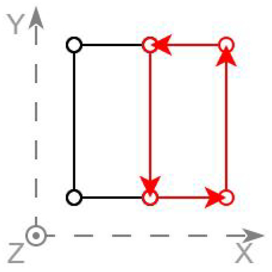
Figure 12.
Structure of generated 3D definition.
2.2. Computer Vision Integration
Even though computer vision methods are usually time-consuming, the accuracy provided by those methods is worth the effort. This integration is exclusively used to generate real urban environments using OSM information. The computer vision framework Building Recognition using AI at Large-Scale (BRAILS) [33,34] is used. It is a Python 3 project using deep learning designed to resolve data scarcity. One of BRAILS modules is integrated into the generation process, as a method to recognize the basic roof shapes, when OSM does not provide them.
2.2.1. Roof Shape Classifier
The Roof Shape Classifier is one of the BRAILS modules, used to obtain the name of the roof shape for each particular building. To use the module, the input for each building to the convolutional neural network is a satellite image of dimension 256 × 256, natively as an image loaded from disk.
The module contains not all the possible roof shapes, but the three major shapes. These shapes are flat, gabled, and hipped. They are 87.49% of all the tagged buildings in OSM [35] (this percentage is obtained at the writing time, but it may have little variations with time).
As with all other modules in the framework, the neural network is trained with the ConvNet technique, using images retrieved using Google Maps API, and validating the results with existing tags provided by OSM. ConvNet is a supervised learning algorithm, a class of deep neural network inspired by biological processes, most commonly applied to analyzing images. This module specifically uses a ResNet [36] with 50 layers.
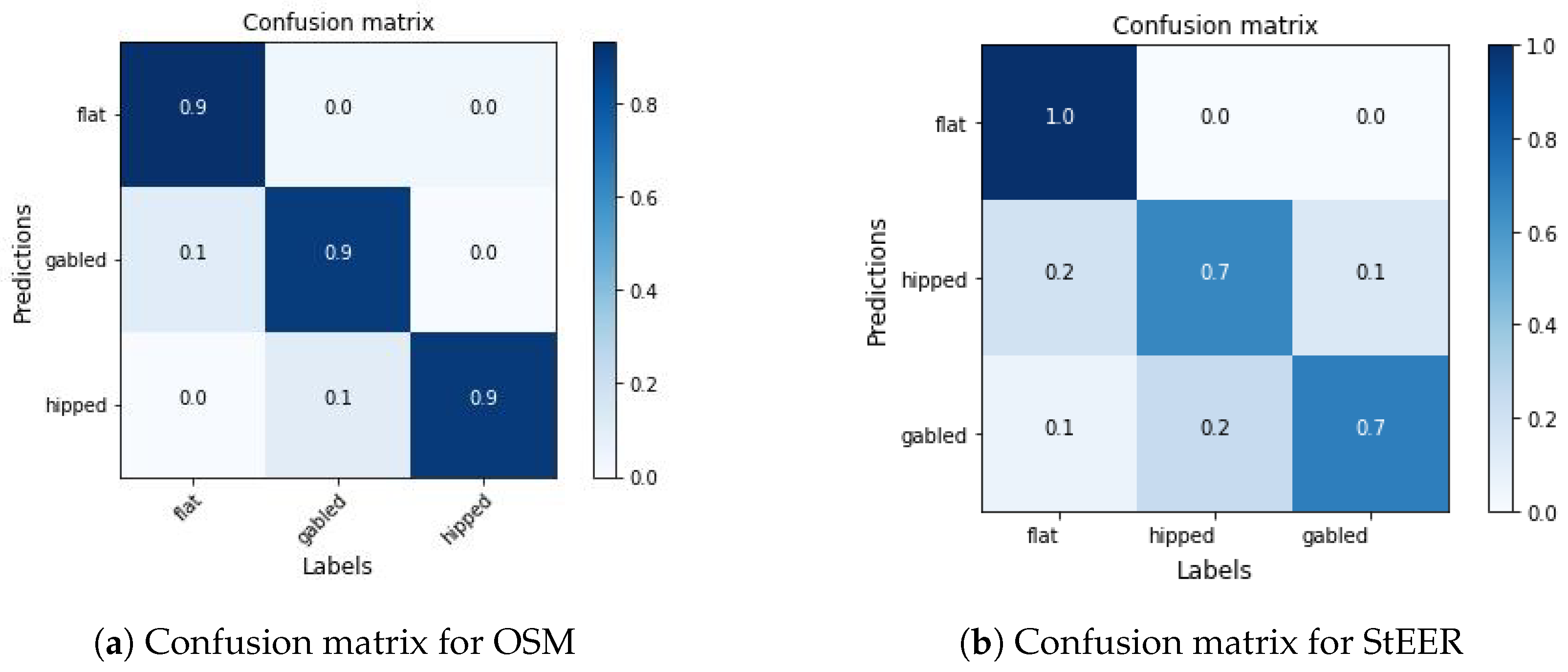
The results are validated by existing tags provided by OSM and labels in the StEER [37] Hurricane Laura Dataset. So, for the validation, only the roofs with these shapes can be used, the buildings are selected randomly, removing the ones whose roofs are not visible from the satellite image for any reason (normally, when covered by trees). The validation of the network obtains the classification metrics in Table 1 and the confusion matrices in Figure 13.

Table 1.
Classification metrics for neural network validation.
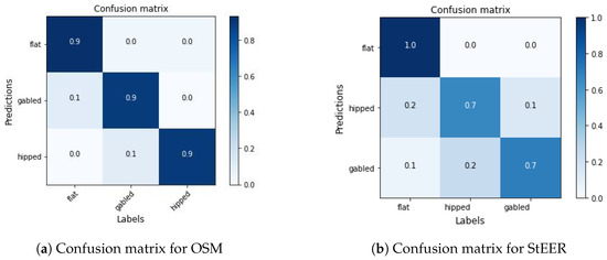
Figure 13.
Confusion matrices for neural network validation.
According to Table 1, the classifier model shows exceptional performance for OSM building entities across all metrics, indicating that it reliably classifies the visible roofs. The model effectively minimizes both false positives and false negatives, with equal values for precision, recall, and the F1-score. This suggests that the model can accurately identify roof shapes and is robust against the challenges of this validation dataset. The high metrics imply that the model generalizes well within the context of the selected roofs, likely due to its training being well-aligned with the validation criteria. Using this model is ideal for this work.
The validation with the StEER dataset shows lower performance metrics, indicating challenges in accurately classifying its roofs. The StEER metrics have low differences, indicating that while the model attempts to balance false positives and false negatives during its training, it still falls short in both areas compared to the OSM results. This suggests difficulties in correctly identifying the StEER roof shapes. The F1-score is slightly higher than precision and recall, indicating some improvement in the model performance when considering the balance between precision and recall.
The generation process may create a task for this module for each building group. Such creation happens when some roof shapes are not provided and no building parts exist in the group. This last filter can avoid the amount of unnecessary computational efforts, because the accuracy of the classifier is low for this kind of complex building, and most building parts are only part of the footprint with different levels, having a flat roof.
The generation process should be completely automatic and parallelizable for multiple tasks. The classifier needs to be specified to achieve these requirements. First, images to be loaded directly from the memory are made, and then the usage of shared memory for any dynamic content is removed in the original implementation.
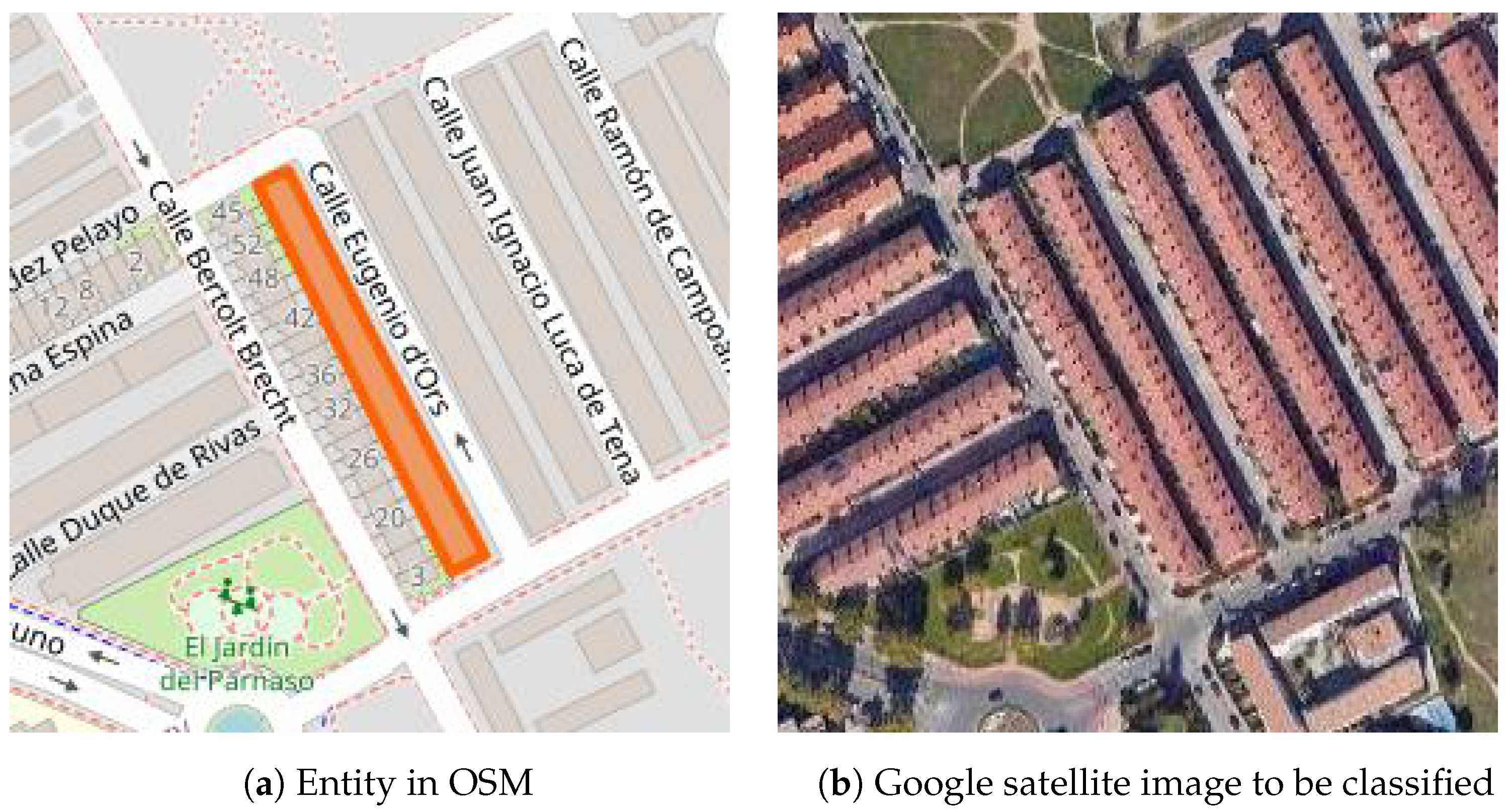
2.2.2. Obtaining the Images
Another requirement for a completely automatic generation process is the method to obtain the input images for the classifier. The solution adopted is Google Satellite Images, which is used natively by the framework to train the model, and the tile images provided also have dimensions of 256 × 256.
The images obtained should only be in the satellite view, ignoring any location labels.
The implemented method to obtain the images needs only the Mercator bounding box of the building footprints, which can be obtained easily by calculating the maximum and minimum value of the footprint coordinates.
First, reflect the border coordinates (left, bottom, right, top) into the overall world position, with a range of , using Equation (8). The left and right positions correspond with x, and the bottom and top with y; the values in the denominator are the bounding ranges of the Mercator projection.
Adapting to the data structure of Google Satellite, it has 22 zoom levels, indexed by two dimensions independently for each level. The zoom level is an integer value inversely proportional to the area dimension on the world map. For a bounding box, the required zoom level is the maximum zoom to contain the building footprint floor to an integer, and it is obtained using the previously obtained world position with the Equation (9),
Level 20 is the standard zoom for building details according to Google documentation. This method sets the upper zoom level to this value. Extreme zooms of level 21 or 22 are rarely used and do not provide more accuracy to the neural network. For these reasons, the buildings with tiny dimensions also use tiles of zoom level 20, where the same tile can intersect with many buildings, reducing the number of Google tiles requested.
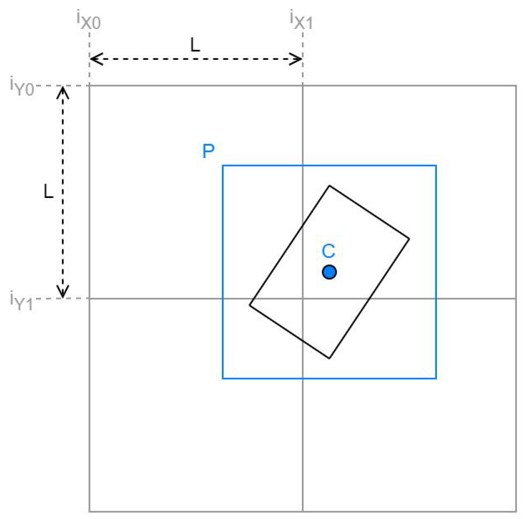
For the best performance of roof classification, the images obtained should have the building at the center, but this is improbable for the tile images of Google Satellite. Four different tiles should be concatenated and cropped to gain an image with the building centered.
Taking the center point indexing for the zoom level as the reference, obtained as C in Equation (10). The tiles to be concatenated have the indexes of , , and calculated with Equation (11).
Finally, this image with a dimension of 512 × 512 concatenated, is cropped starting with the pixel P obtained in Equation (12) to obtain the final 256 × 256 image.
All the above details are shown in Figure 14. The black rectangle is the building, the grey boxes are the satellite tiles, and the blue box is the final image. The dimension L is 1 for tiles indexing and 256 for image pixels.
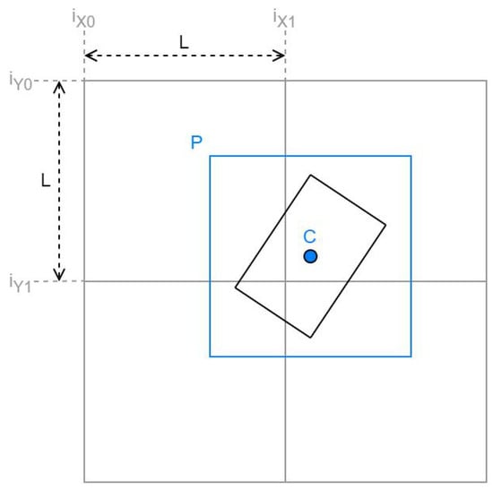
Figure 14.
Tiles concatenation and cropping for building to obtain an image to classify a roof.
2.3. Custom Environment Generation
This subsection explains the possibility of usage of the method in different ways. Creating an environment should never be completely manual, with only slight modifications needed to existing definitions.
Procedural generation is commonly used to create models for urban environments [4,14], whose most important part of the output information is the positioning of the urban objects on a map, including the building footprints and the roof shapes. The method can use this information to generate the 3D model, as a black box, allowing procedural generation without detailed 3D management.
Another possible approach to utilizing the method involves modifying information obtained from data mining tools, such as extracting the OSM information and manually editing any incorrect parameters like the roof shapes of building entities.
The information required is similar to the creation of a real environment: the ground grid, the building 2D footprints, the roof shapes, the building total heights, the building roof heights, and the colors and materials of the building faces. The presence of an intersection should also group the building entities if it is important for the generated model.
2.4. Implementation
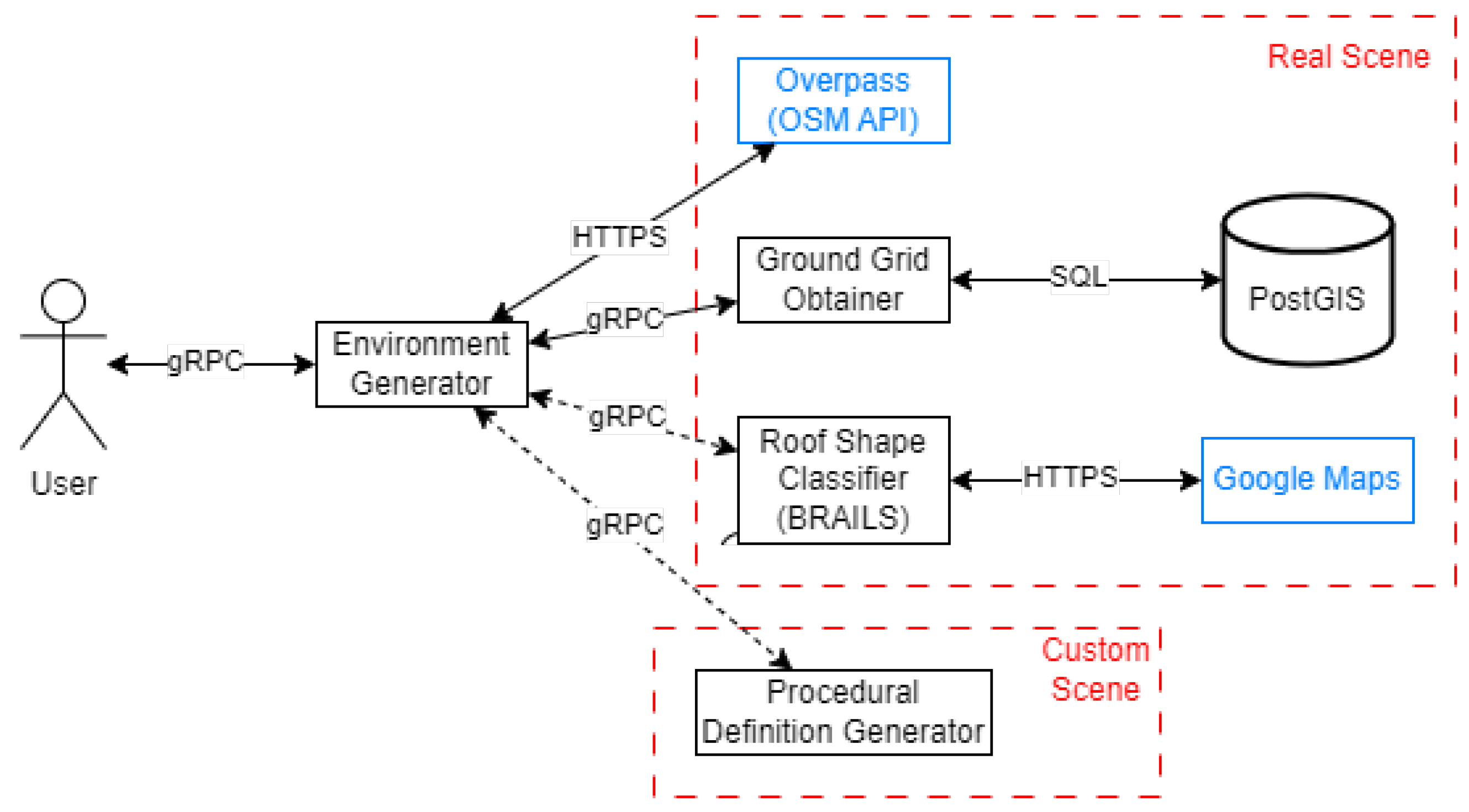
The system is implemented based on the general Remote Procedure Calls (gRPC) framework, allowing communication between different programming languages, including external requests (see Figure 15).
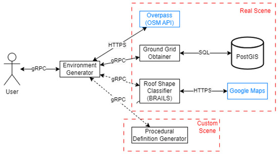
Figure 15.
Component diagram of the implementation.
The models are obtained by calling the gRPC server of the main generation process, which is responsible for calling any other method.
The elevation values from SRTM raster data are extracted and stored in a PostgreSQL server to allow fast obtaining of the ground grid. The SQL server contains the module PostGIS, using its intersection function for the queries. A gRPC server implements the needed SQL queries.
The OSM building information is obtained by HTTP request to the Overpass API, requesting the output in JSON format.
A gRPC server in Python implements the Roof Shape Classifier of the BRAILS module, including the requests for the Google Satellite images.
Another gRPC server implements a simple procedural generation process, to test the method for creating custom environments.
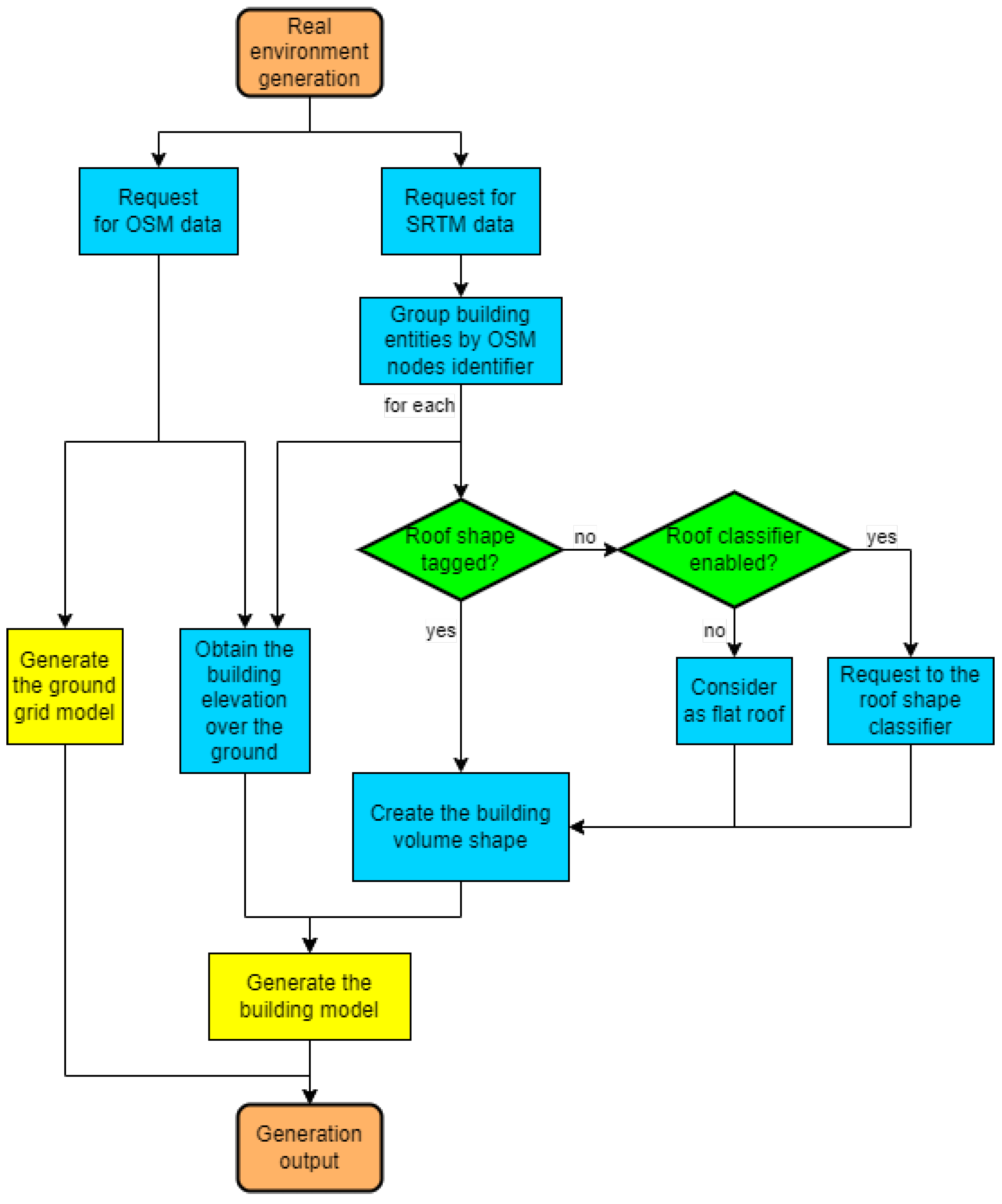
The process of generating a real scene is displayed in Figure 16. The process for custom scenes is one step, considering the “procedural definition generator” as a black box.

Figure 16.
Flowchart to generate a real scene.
3. Results
This section includes the screenshots of the output models from the method, mostly saved in Graphics Library Transmission Format (GLTF) and displayed in Microsoft 3D Viewer version 7.2407.16012.0.
The 3D meshes in GLTF have the Y-axis for the altitude and face vertices in counter-clockwise order. The vertices in GLTF have coordinates with position shift compared to the method output, the Z-axis for altitude used in the method becomes the Y in GLTF, Y becomes X, and X becomes Z. The triangle indexing array can be used directly without conversion, and GLTF supports color mode by faces.
3.1. Concrete Buildings
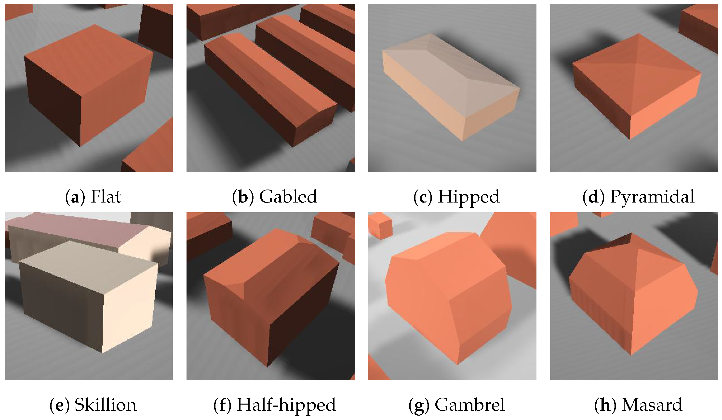
Several generated models are illustrated in Figure 17, for each considered roof shape. These buildings are individuals, generated from a single and independent building entity.

Figure 17.
Examples of single building by roof shapes.
Figure 18 shows two buildings of the University of Alcala (UAH), whose definition is the combination of multiple building entities. Each entity with the tag “building:part” represents a different height value for a section of the footprint coordinate.
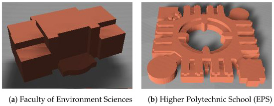
Figure 18.
Examples of complex buildings.
3.2. Ground Grid
Normally, the contrast of elevation of the ground grid model is not obvious in urban scenes. Each tile has approximately 3/4 hectares and can contain many buildings, most of the building entities are covered by up to 2 ground tiles, and even large buildings such as the UAH EPS (Figure 18b) are covered by only 9 tiles. It is not easy to perceive the ramps when there are many buildings.
If multiple buildings with the same height are consecutive in the generated model, a step shape can be found in their roof faces when they are over a ramp.
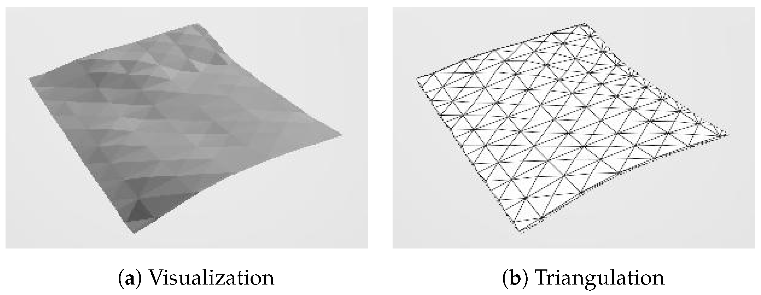
A small mountain area was chosen to represent the generated ground grid in Figure 19, where the elevation values have enough contrast and no building entities exist.
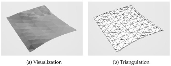
Figure 19.
Example of the ground model only, with tiles divided by diagonals.
3.3. Real Environment Generation
This section shows the generated models of two real urban areas and compares the resulting model with CV applied or not.
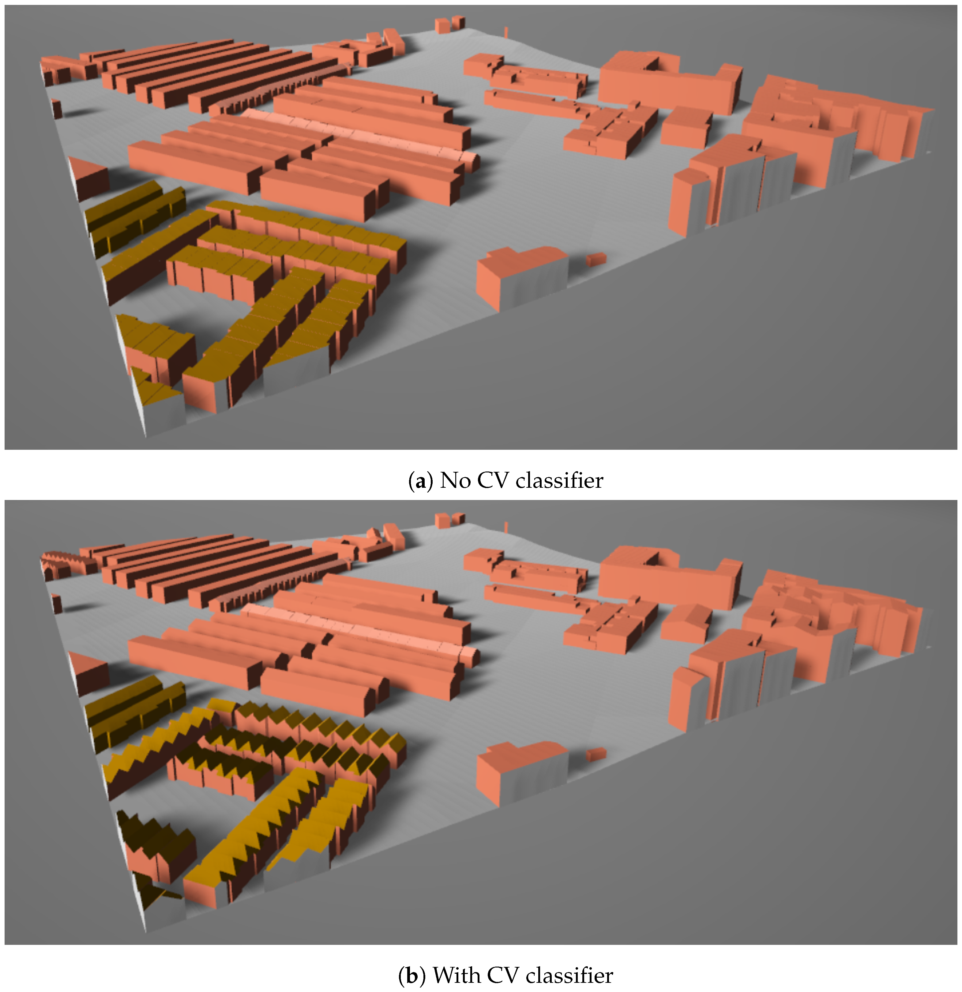
The scene in Figure 20 has 210 buildings in the area, 59 of which have the roof shape provided by OSM, all of these are gabled. A total of 147 can be classified using the CV in the remaining buildings, resulting in 59 flats, 74 gabled, and 14 hipped. The statistical comparison is displayed in Table 2.
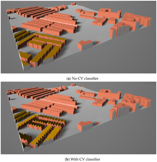
Figure 20.
Real scene example: Alcala de Henares.
Table 2.
Generation statistics: Alcala de Henares.
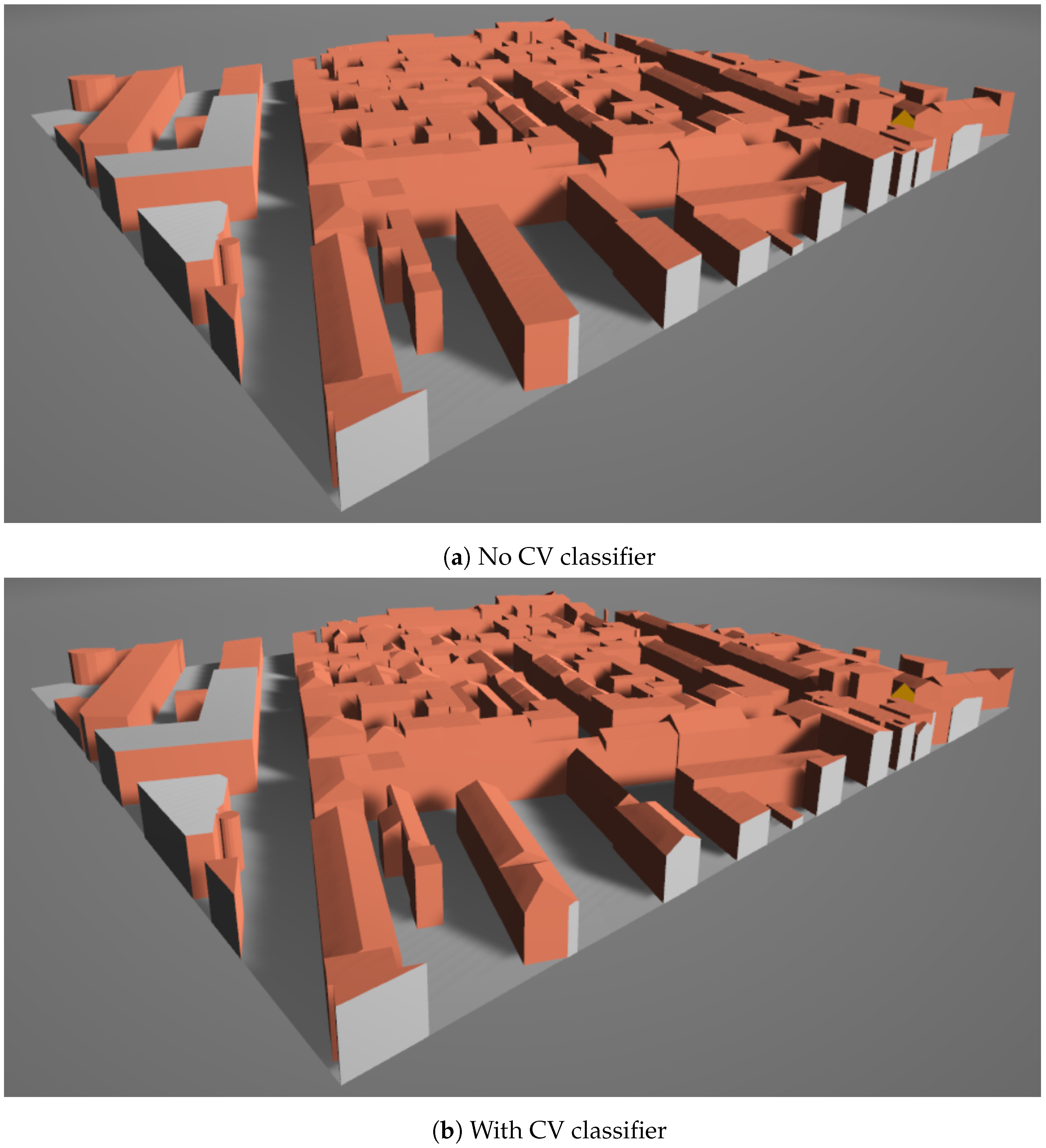
Another scene in Figure 21 has 174 buildings in the area, 56 of which have the roof shape provided by OSM, 54 gabled, 1 hipped, and 1 pyramidal. A total of 112 can be classified using the CV in the remaining buildings, resulting in 54 flats, 49 gabled, and 9 hipped. The statistical comparison is displayed in Table 3.
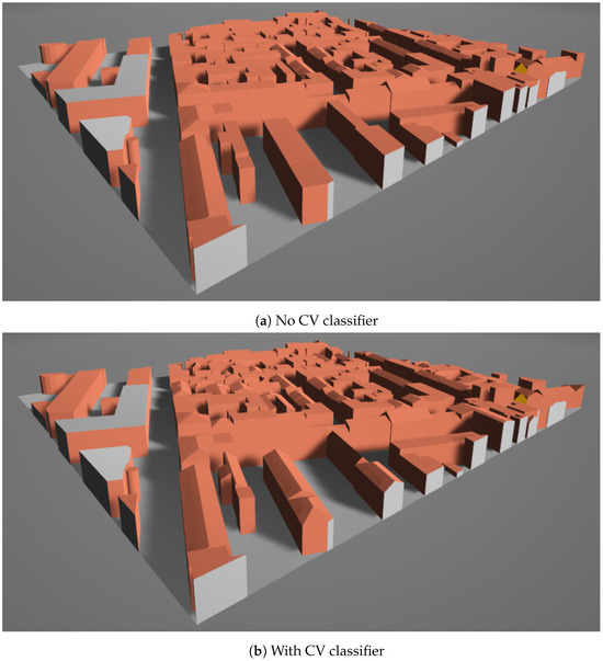
Figure 21.
Real scene example: Munich.
Table 3.
Generation statistics: Munich.
In both cases, the CV extension obtained the majority of the roofs; its application improved the model details and caused a considerable increase in time consumption. The discrepancy between the results corresponds to the difference between the proportion of flat roofs, considering that all unclassified roofs are generated as flat roofs when CV is not applied. Most of the time, the OSM data do not tag the buildings with flat roofs, but this shape should be the majority in the world, but the number of these tags in OSM is less than for the gabled [35].
3.4. Custom Environment Generation
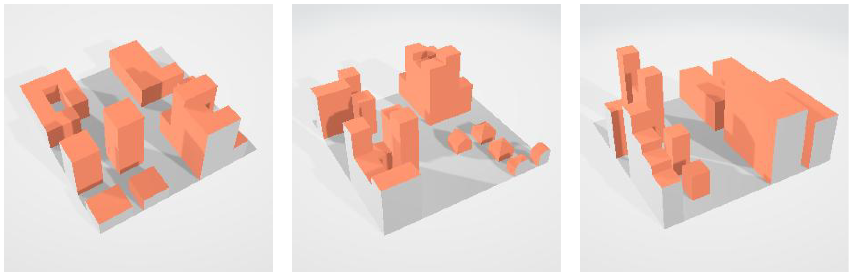
As mentioned before, the input information to the method is the positioning of the urban objects on a map, including the building footprints and the roof shapes. A simple procedural generation program is used to create this information to test the method.
The generation is based on ground layouts, picked randomly. The buildings in each layout can have flattened or shaped roof shapes, the same or different heights, and have consecutive or separated positioning.
The ground grid generation is not included, so the generated 3D model will have a flat ground.
The following parameters are required to proceed with a procedural generation:
- 2D area dimension
- Scene complexity, dividing the scene into approximately layouts
- The weight of each building layout
- The weight of each roof shape when the picked layout does not have flattened roof shapes
Figure 22 displays three examples generated with dimensions of 20 × 20, scene complexity 2, same layout weights, and roof shape weights predominately gabled.

Figure 22.
Examples of procedural generation.
3.5. Unity Rendering
Rendering a scene in Unity consists of calling the gRPC service of the main generation process, and adapting the geometry format to the 3D mesh definition of Unity.
In all versions of Unity, the supported .NET version can not directly include gRPC as a dependency. The solution to implementing a gRPC client is to create a dynamic library written in C++ and compiled for the operating system required. The Unity scripts should be able to complete the gRPC communication by importing the minimum number of functions, which must be declared to follow the calling convention of the C language.
The 3D meshes in Unity have the Y-axis for the altitude and face vertices in clockwise order. The vertices in Unity have the coordinates Y and Z swapped compared to the method output, and the color array has a corresponding value for each vertex. The triangle indexing array in Unity is reversed compared to the method output. These functionalities can become a Unity package.
Figure 23 rendered in Unity Engine the same scene as Figure 20a, rotated approximately 105 degrees clockwise.
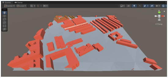
Figure 23.
Example of Unity rendering.
4. Discussion
This section will discuss the method’s achievement and its results concerning the hypothesis.
The proposed method is cost-effective under standalone execution. It generates each square kilometer of scene taking around 10 s.
Regarding the first hypothesis, “the approach of creating a universal method to generate building models over a ground grid,” is already demonstrated in Section 3. The proposed method is used to create models for two different formats, GLTF and Unity.
Regarding the second hypothesis, “appropriateness of creating the real urban environments, using SRTM and OSM information as input to the method”, the SRTM dataset chosen has a rectangular grid for each 1/1200 of latitude or longitude, and this precision is enough for urban areas with low differences in ground elevation. OSM is a great source for 2D building information, but it has some limitations for the altitudes and shapes due to information incompleteness. A few building entities have a shape for their bottom face, which is not defined in OSM.
Compared to combining DSM and DTM for building heights, the OSM information has the advantage of the speed of obtaining values, specifically when the roof has pitched faces. If the combination obtains only the average value for the height, it can only generate flat roofs [3,9]. However, when OSM does not provide the heights for some building entities, there is no easy way to fill them. OSM can be used everywhere in the world even though the information is incomplete, and using DSM requires datasets with very-high-precision grids by decimeters.
Concerning the third point, “effectiveness of integration of computer vision to the method to improve the quality of the model generated”, most of the time, the classification accuracy is acceptable as the matrices provided by BRAILS (Figure 13) add roof shape details to the generated model. However, there is a problem in its combination with OSM. Some building entities represent multiple buildings in a row, and the lengths of the sides differ greatly, as illustrated in Figure 24. In the satellite image used as input to the CV, the area coverage of the entity is too small and causes a low weight, making the classification almost impossible. There are many entities of this type in the scene example of Alcala (Figure 20).
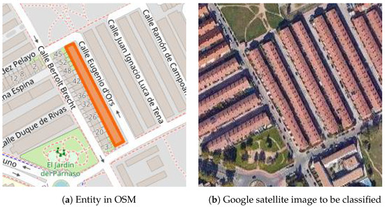
Figure 24.
Multiple buildings in a row as single OSM entity. I do not understand. It is complete.
Regarding the fourth point, “usability of the method for environments with procedurally generated or user custom definitions”, this is already demonstrated by the test in Section 3.4. The method functionality is very stable providing all the information needed.
5. Conclusions
This paper proposed a 3D mesh generation method that can be adapted to different file formats and environments, designed for models of ground and buildings with roof shapes in urban environments. It can be useful for research that combines multiple models, allowing a combination using the structure of any other. The generation is mainly applied to real urban scenes worldwide, taking the available geographic information, obtained directly or by performing calculations. The models are optimized by making volume unions and computer vision classification using satellite images. There is also the possibility of using the method to generate scenes using custom definitions; these definitions can be decisions on the planning process or information from real scenes slightly modified when any mistake is detected.
However some complementary ideas have not been completed during this work, and future research may complete them.
For the geometric processing to adapt footprint shapes to rectangular (Figure 6), the initial plan was to complete both ways and have a selection theory for each building entity. However, only the first way to crop a single rectangle was performed and applied in the method.
The polygon-covering algorithm using rectangles is the first step to achieving that. A partial method that considers possible noise sides was used, with pending problems. First, this method did not consider inner holes in the building footprint. Second, the final model should be the volumetric union of the models generated from each cover rectangle, and it is hard to align the vertices for most of the roof shapes. A problematic example is displayed in Figure 25, where the generated model has too many redundant edges.
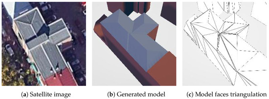
Figure 25.
Example of modeling by polygon-covering.
The other pending problem is to fill the building height values when OSM has missing values in some building entities. Sometimes, when OSM does not provide the height values directly, it can be estimated by related tags, such as “building:levels” and “roof:levels”, considering each level to have a height between 3 and 4 m. However, OSM still contains numerous building entities that lack valid height information.
This problem may be addressed by applying computer vision to street view images or finding a global DSM and DTM with enough geographic precision.
Author Contributions
Conceptualization, H.L. and C.J.H.; methodology, H.L.; software, H.L. and C.D.; validation, C.D.; investigation, H.L.; writing—original draft preparation, H.L.; writing—review and editing, C.J.H., A.T., C.D. and J.G.; visualization, H.L.; supervision, C.J.H., A.T. and J.G.; project administration, A.T.; funding acquisition, J.G. All authors have read and agreed to the published version of the manuscript.
Funding
This work was supported by the program “Programa de Estímulo a la Excelencia para Profesorado Universitario Permanente” of Vice Rectorate for Research and Knowledge Transfer of the University of Alcala and by the Comunidad de Madrid (Spain) through project EPU-INV/2020/004.
Data Availability Statement
Data are contained within the article.
Conflicts of Interest
The authors declare no conflicts of interest.
Abbreviations
The following abbreviations are used in this manuscript:
| API | Application Programming Interfaces |
| GIS | Geographic Information System |
| DSM | Digital Surface Model |
| DTM | Digital Terrain Model |
| AI | Artificial Intelligence |
| CIM | City Information Model |
| CV | Computer Vision |
| NeRF | Neural Radiant Field |
| SRTM | Shuttle Radar Topography Mission |
| OSM | OpenStreetMap |
| DLF | Descending Level Function |
| HE | Hip Elevation |
| GP | Gambrel Portion |
| MP | Mansard Portion |
| BRAILS | Building Recognition using AI at Large-Scale |
| gRPC | general Remote Procedure Calls |
| GLTF | Graphics Library Transmission Format |
| EPS | Higher Polytechnic School |
| UAH | University of Alcala |
Appendix A. Roof Shapes
The appendix contains the details for each roof shape defined in OSM according to the theory explained in Section 2.1.3.
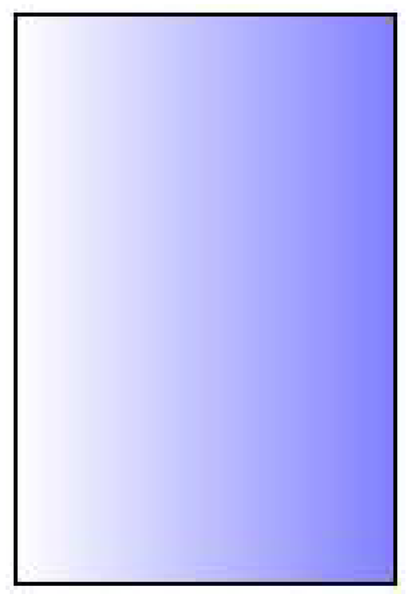
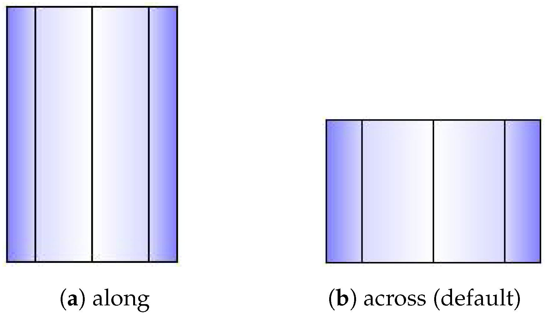
Appendix A.1. Gabled
This roof shape uses one coordinate for DLF. This coordinate will be chosen by the property “orientation” of the building entity. when it is “along”, when it is “across”, default to “along” when the property is not provided (Figure A1).
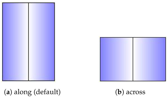
Figure A1.
Shape of gabled roof.
Figure A1.
Shape of gabled roof.

Side dividing segments:
Virtual roof polygons:
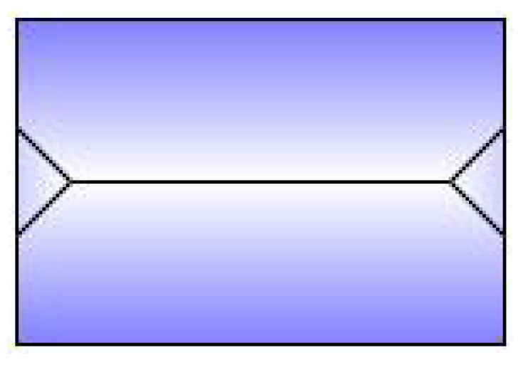
Appendix A.2. Hipped
This roof shape uses both coordinates for DLF, with a specific alternative value obtained for each building entity:
This value ensures 45 degrees for inclined angles in Figure A2.
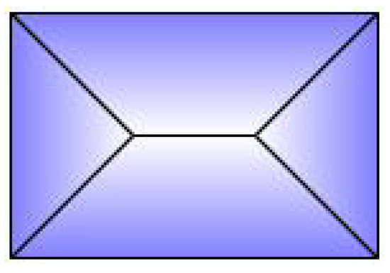
Figure A2.
Shape of hipped roof.
Figure A2.
Shape of hipped roof.
Side dividing segments:
Virtual roof polygons:
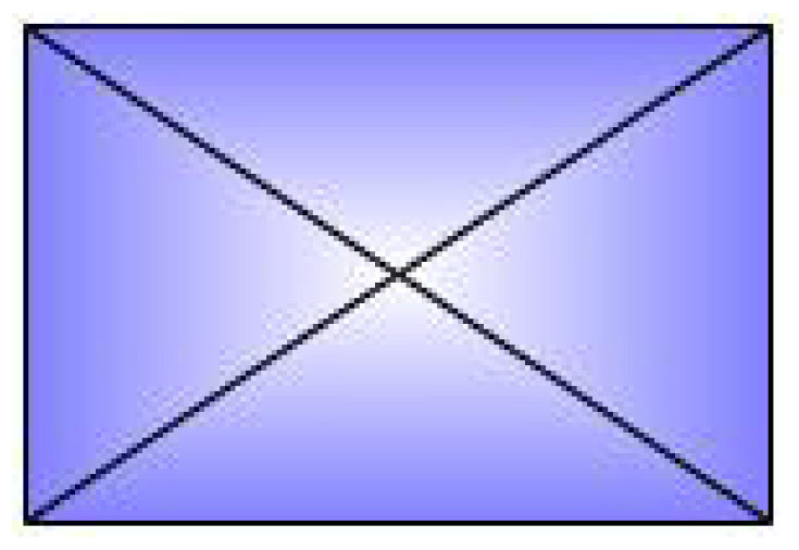
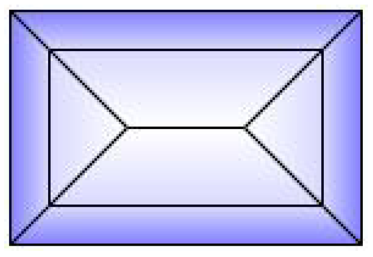
Appendix A.3. Pyramidal
This roof shape uses both coordinates for DLF (Figure A3).
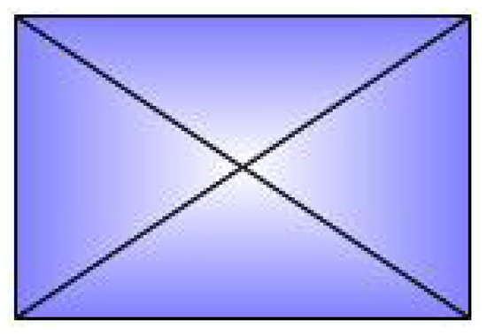
Figure A3.
Shape of pyramidal roof.
Figure A3.
Shape of pyramidal roof.
Side dividing segments:
Virtual roof polygons:
Appendix A.4. Skillion
This roof shape is a particular case. The alternative coordinate is not obtained by walking through the outer sides of the footprint. The building entity should include a property named “direction” to represent the alternative coordinate direction. The property gives an angle in degrees (it should be converted to radians normally), starting from the north and rotating clockwise.
There is only one roof polygon, and the side segments do not need to be divided (Figure A4). The 2D coordinates of the polygon are equal to the building footprints and do not need to have an intersection with virtual roof polygons.
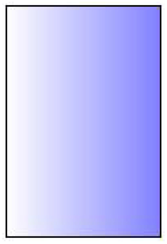
Figure A4.
Shape of skillion roof.
Figure A4.
Shape of skillion roof.
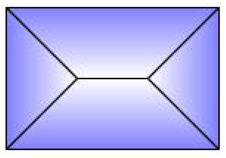
Appendix A.5. Half-Hipped
An algorithm parameter Hip Elevation (HE) is used for this roof shape, which determines the height fraction of hips on the lateral sides to be elevated. Its value must be between 0 and 1, typically greater than 0.5. When , the result will be the same as a hipped roof. When , the result will be the same as a gabled roof with orientation “along”. The recommended value is 0.7 (Figure A5).
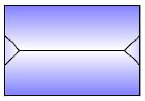
Figure A5.
Shape of half-hipped roof.
Figure A5.
Shape of half-hipped roof.
This roof shape uses both coordinates for DLF, with these specific alternative values obtained for each building entity:
Side dividing segments:
Virtual roof polygons:
Appendix A.6. Gambrel
An algorithm parameter Gambrel Portion (GP) is used for this type of roof, which determines the length fraction in the coordinates where the raised edge should be situated on both hips. Its value must be between 0.5 and 1. When , the result will be the same as a gabled roof; when , the result will be the same as a flat roof. The recommended value is 0.7.
This roof shape uses one coordinate for DLF, this coordinate will be chosen by the property “orientation” of the building entity. when it is “along”, when it is “across”, default to “across” when the property is not provided (Figure A6).
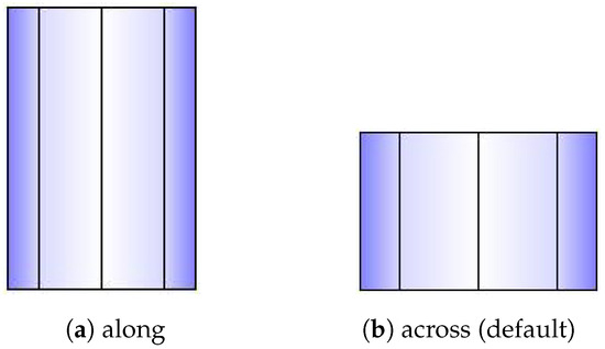
Figure A6.
Shape of gambrel roof.
Figure A6.
Shape of gambrel roof.
Side dividing segments:
Virtual roof polygons:
Appendix A.7. Mansard
An algorithm parameter Mansard Portion (MP) is used for this type of roof, which determines the length fraction in the coordinates where the raised edge should be situated on all the hips. Its value must be between 0.5 and 1. When , the result will be the same as a hipped roof; when , the result will be the same as a flat roof. The recommended value is 0.7 (Figure A7).
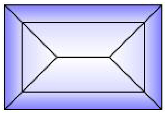
Figure A7.
Shape of mansard roof.
Figure A7.
Shape of mansard roof.
This roof shape uses both coordinates for DLF, with these specific alternative values obtained for each building entity:
Side dividing segments:
Virtual roof polygons:
References
- Gómez, J.; Tayebi, A.; Hellín, C.J.; Valledor, A.; Barranquero, M.; Cuadrado-Gallego, J.J. Accelerated Ray Launching Method for Efficient Field Coverage Studies in Wide Urban Areas. Sensors 2023, 23, 6412. [Google Scholar] [CrossRef] [PubMed]
- Gómez, J.; Hellín, C.J.; Valledor, A.; Barranquero, M.; Cuadrado-Gallego, J.J.; Tayebi, A. Design and Implementation of an Innovative High-Performance Radio Propagation Simulation Tool. IEEE Access 2023, 11, 94069–94080. [Google Scholar] [CrossRef]
- Girindran, R.; Boyd, D.S.; Rosser, J.; Vijayan, D.; Long, G.; Robinson, D. On the Reliable Generation of 3D City Models from Open Data. Urban Sci. 2020, 4, 47. [Google Scholar] [CrossRef]
- Alomía, G.; Loaiza, D.; Zùñiga, C.; Luo, X.; Asoreycacheda, R. Procedural modeling applied to the 3D city model of Bogota: A case study. Virtual Real. Intell. Hardw. 2021, 3, 423–433. [Google Scholar] [CrossRef]
- Egea-Lopez, E.; Molina-Garcia-Pardo, J.M.; Lienard, M.; Degauque, P. Opal: An open source ray-tracing propagation simulator for electromagnetic characterization. PLoS ONE 2021, 16, e0260060. [Google Scholar] [CrossRef]
- Somanath, S.; Naserentin, V.; Eleftheriou, O.T.; Sjölie, D.; Wästberg, B.S.; Logg, A. On procedural urban digital twin generation and visualization of large scale data. arXiv 2023, arXiv:2305.02242. [Google Scholar]
- Ma, Y.P. Extending 3D-GIS District Models and BIM-Based Building Models into Computer Gaming Environment for Better Workflow of Cultural Heritage Conservation. Appl. Sci. 2021, 11, 2101. [Google Scholar] [CrossRef]
- Buyukdemircioglu, M.; Kocaman, S. Reconstruction and Efficient Visualization of Heterogeneous 3D City Models. Remote. Sens. 2020, 12, 2128. [Google Scholar] [CrossRef]
- Pepe, M.; Costantino, D.; Alfio, V.S.; Vozza, G.; Cartellino, E. A Novel Method Based on Deep Learning, GIS and Geomatics Software for Building a 3D City Model from VHR Satellite Stereo Imagery. ISPRS Int. J.-Geo-Inf. 2021, 10, 697. [Google Scholar] [CrossRef]
- Rantanen, T.; Julin, A.; Virtanen, J.P.; Hyyppä, H.; Vaaja, M.T. Open Geospatial Data Integration in Game Engine for Urban Digital Twin Applications. ISPRS Int. J.-Geo-Inf. 2023, 12, 310. [Google Scholar] [CrossRef]
- Knodt, J.; Baek, S.; Heide, F. Neural Ray-Tracing: Learning Surfaces and Reflectance for Relighting and View Synthesis. arXiv 2021, arXiv:2104.13562. [Google Scholar]
- Garifullin, A.; Maiorov, N.; Frolov, V.A. Single-view 3D reconstruction via inverse procedural modeling. arXiv 2023, arXiv:2310.13373. [Google Scholar]
- Biancardo, S.A.; Capano, A.; de Oliveira, S.G.; Tibaut, A. Integration of BIM and Procedural Modeling Tools for Road Design. Infrastructures 2020, 5, 37. [Google Scholar] [CrossRef]
- Bulbul, A. Procedural generation of semantically plausible small-scale towns. Graph. Model. 2023, 126, 101170. [Google Scholar] [CrossRef]
- Tytarenko, I.; Pavlenko, I.; Dreval, I. 3D Modeling of a Virtual Built Environment Using Digital Tools: Kilburun Fortress Case Study. Appl. Sci. 2023, 13, 1577. [Google Scholar] [CrossRef]
- Kim, S.; Kim, D.; Choi, S. CityCraft: 3D virtual city creation from a single image. Vis. Comput. 2020, 36, 911–924. [Google Scholar] [CrossRef]
- La Russa, F.M.; Grilli, E.; Remondino, F.; Santagati, C.; Intelisano, M. Advanced 3D Parametric Historic City Block Modeling Combining 3D Surveying, AI and VPL. Int. Arch. Photogramm. Remote. Sens. Spat. Inf. Sci. 2023, XLVIII-M-2-2023, 903–910. [Google Scholar] [CrossRef]
- Starzyńska-Grześ, M.B.; Roussel, R.; Jacoby, S.; Asadipour, A. Computer Vision-based Analysis of Buildings and Built Environments: A Systematic Review of Current Approaches. ACM Comput. Surv. 2023, 55, 1–25. [Google Scholar] [CrossRef]
- Shahzad, M.; Maurer, M.; Fraundorfer, F.; Wang, Y.; Zhu, X.X. Buildings Detection in VHR SAR Images Using Fully Convolution Neural Networks. IEEE Trans. Geosci. Remote. Sens. 2019, 57, 1100–1116. [Google Scholar] [CrossRef]
- Zhou, X.; Sun, K.; Wang, J.; Zhao, J.; Feng, C.; Yang, Y.; Zhou, W. Computer Vision Enabled Building Digital Twin Using Building Information Model. IEEE Trans. Ind. Inform. 2023, 19, 2684–2692. [Google Scholar] [CrossRef]
- García-Gago, J.; González-Aguilera, D.; Gómez-Lahoz, J.; San José-Alonso, J.I. A Photogrammetric and Computer Vision-Based Approach for Automated 3D Architectural Modeling and Its Typological Analysis. Remote. Sens. 2014, 6, 5671–5691. [Google Scholar] [CrossRef]
- Faltermeier, F.L.; Krapf, S.; Willenborg, B.; Kolbe, T.H. Improving Semantic Segmentation of Roof Segments Using Large-Scale Datasets Derived from 3D City Models and High-Resolution Aerial Imagery. Remote. Sens. 2023, 15, 1931. [Google Scholar] [CrossRef]
- Ruiz de Oña, E.; Barbero-García, I.; González-Aguilera, D.; Remondino, F.; Rodríguez-Gonzálvez, P.; Hernández-López, D. PhotoMatch: An Open-Source Tool for Multi-View and Multi-Modal Feature-Based Image Matching. Appl. Sci. 2023, 13, 5467. [Google Scholar] [CrossRef]
- Gao, K.; Gao, Y.; He, H.; Lu, D.; Xu, L.; Li, J. NeRF: Neural Radiance Field in 3D Vision, A Comprehensive Review. arXiv 2022, arXiv:2210.00379. [Google Scholar]
- Eller, L.; Svoboda, P.; Rupp, M. A Deep Learning Network Planner: Propagation Modeling Using Real-World Measurements and a 3D City Model. IEEE Access 2022, 10, 122182–122196. [Google Scholar] [CrossRef]
- Gong, X.; Su, T.; Zhao, W.; Chi, K.; Yang, Y.; Yao, C. A Potential Game Approach to Multi-UAV Accurate Coverage Based on Deterministic Radio Wave Propagation Model in Urban Area. IEEE Access 2023, 11, 68560–68568. [Google Scholar] [CrossRef]
- Alwajeeh, T.; Combeau, P.; Aveneau, L. An Efficient Ray-Tracing Based Model Dedicated to Wireless Sensor Network Simulators for Smart Cities Environments. IEEE Access 2020, 8, 206528–206547. [Google Scholar] [CrossRef]
- Choi, H.; Oh, J.; Chung, J.; Alexandropoulos, G.C.; Choi, J. WiThRay: A Versatile Ray-Tracing Simulator for Smart Wireless Environments. IEEE Access 2023, 11, 56822–56845. [Google Scholar] [CrossRef]
- Hansson Söderlund, H.; Evans, A.; Akenine-Möller, T. Ray Tracing of Signed Distance Function Grids. J. Comput. Graph. Tech. (JCGT) 2022, 11, 94–113. [Google Scholar]
- van Wezel, C.S.; Verschoore de la Houssaije, W.A.; Frey, S.; Kosinka, J. Virtual Ray Tracer 2.0. Comput. Graph. 2023, 111, 89–102. [Google Scholar] [CrossRef]
- Jarvis, A.; Reuter, H.; Nelson, A.; Guevara, E. Hole-Filled SRTM for the Globe Version 4. CGIAR-CSI SRTM 90m Database. 2008. Available online: https://csidotinfo.wordpress.com/data/srtm-90m-digital-elevation-database-v4-1/ (accessed on 20 October 2024).
- OpenStreetMap Contributors. Planet Dump. 2017. Available online: https://planet.osm.org (accessed on 20 October 2024).
- Cetiner, B.; Wang, C.; McKenna, F.; Hornauer, S.; Zhao, J.; Guo, Y.; Yu, S.X.; Taciroglu, E.; Law, K.H. BRAILS Release v3.1.0. 2024. Available online: https://zenodo.org/records/10448047 (accessed on 20 October 2024).
- Deierlein, G.G.; McKenna, F.; Zsarnóczay, A.; Kijewski-Correa, T.; Kareem, A.; Elhaddad, W.; Lowes, L.; Schoettler, M.J.; Govindjee, S. A Cloud-Enabled Application Framework for Simulating Regional-Scale Impacts of Natural Hazards on the Built Environment. Front. Built Environ. 2020, 6, 558706. [Google Scholar] [CrossRef]
- OpenStreetMap Contributors. Roof:Shape|OpenStreetMap TagInfo. 2024. Available online: https://taginfo.openstreetmap.org/keys/roof:shape#values (accessed on 24 May 2024).
- He, K.; Zhang, X.; Ren, S.; Sun, J. Deep Residual Learning for Image Recognition. In Proceedings of the 2016 IEEE Conference on Computer Vision and Pattern Recognition (CVPR), Las Vegas, NV, USA, 27–30 June 2016; pp. 770–778. [Google Scholar] [CrossRef]
- Gutierrez Soto, M.; Do, T.; Kameshwar, S.; Allen, D.; Lombardo, F.; Roueche, D.; Demaree, G.; Rodriguez, G.E.; LaDue, D.; Palacio-Betancur, A.; et al. 21–22 March 2022 Tornado Outbreak Field Assessment Structural Team Dataset. v1. 2023. Available online: https://www.designsafe-ci.org/data/browser/public/designsafe.storage.published/PRJ-3443/#details-164541364985523730-242ac117-0001-012 (accessed on 20 October 2024).


Disclaimer/Publisher’s Note: The statements, opinions and data contained in all publications are solely those of the individual author(s) and contributor(s) and not of MDPI and/or the editor(s). MDPI and/or the editor(s) disclaim responsibility for any injury to people or property resulting from any ideas, methods, instructions or products referred to in the content. |
© 2024 by the authors. Licensee MDPI, Basel, Switzerland. This article is an open access article distributed under the terms and conditions of the Creative Commons Attribution (CC BY) license (https://creativecommons.org/licenses/by/4.0/).