Sequential and Parallel Algorithms to Compute Turbulent Coherent Structures

Abstract

The behavior of turbulent flows remains a significant unsolved problem in physics. Recently, a large quantity of effort has been directed toward understanding the non-linear interactions of the different flow structures in order to address this challenge. In this paper, different implementations of one exact method for identifying these structures are analyzed. This includes two sequential algorithms and a parallelizable one, developed to handle large-scale data efficiently. The new parallel algorithm offers significant advantages in handling the computational demands of large simulations, providing a more scalable solution for future research.

1. Introduction

Turbulence is arguably considered the most significant unsolved problem in physics, with widespread applications in everyday life. It is estimated that up to 5% of global CO₂ emissions each year are accounted for by wall-bounded turbulence [1]. While fully understanding turbulence may still be an overly ambitious goal that remains far from being achieved [2,3], improving models to reliably and efficiently simulate flow behavior is viewed as a more attainable objective [4]. It should be noted that even an existence and uniqueness theorem for the solution of the Navier–Stokes equations governing fluid flows has yet to be established [5].

To gain a fundamental understanding of turbulent flows, Direct Numerical Simulation (DNS) is widely recognized as one of the most important techniques today, which involves solving the Navier–Stokes Equations [6] without any modeling [7,8]. However, the use of DNS is restricted to simplified geometries due to its immense computational cost [9]. Among these idealized flows, turbulent Poiseuille channel flows, where the flow is confined between two parallel plates and driven by pressure, have been the most successful. Supercomputers have been essential tools for performing these simulations, and the exponential increase in computational power since the 1990s has allowed DNS to advance accordingly. The friction Reynolds number ($R{e}_{\tau }=h{u}_{\tau }/\nu$), the primary control parameter, has been steadily increased since the pioneering work of Kim, Moin, and Moser [7], see [10] and references therein.

In this definition, h is the semi-height of the channel, $\nu$ is the kinematic viscosity, and $u_{\tau }$ is the friction velocity, which is defined as the square root of the stress at the wall. The friction velocity $u_{\tau }$ is a fictitious velocity, meaning it does not physically exist but serves as a fundamental scaling parameter for wall-bounded flows [11].

As a result of this increased size, immense databases have been created. For instance, each velocity field from Hoyas and Oberlack [10] is close to 1 Terabyte (TB). The challenge of obtaining trustworthy and valuable results from these hundreds of terabytes is becoming increasingly difficult.

Over the past century, the primary approach to understanding and modeling turbulence has been through Reynolds decomposition and the refinement of scaling laws [12]. Various techniques and a great deal of ingenuity have been employed [13,14] over the years, but even classical scaling laws continue to be debated. One example is the flow behavior in the so-called logarithmic layer, first described by Von Kármán [15] nearly 90 years ago. Although this concept has been widely applied throughout the last century, it remains a subject of significant debate today; see [16] and references therein.

Several new ideas have emerged, such as the use of symmetry theory [17,18], but a complete understanding has yet to be achieved. In recent years, a shift toward studying turbulent structures has been observed [19]. Structures were first described experimentally as streamwise streaks [20] and Reynolds-stress events [21]. Other structures closely related to the Reynolds stress are the Q-events [22], which are defined as regions of strong momentum flux. Using another point of view, in 1995, Chong et al. [23] provided a mathematical definition of vortexes, roughly identifying them as regions with more vorticity than shear. Nevertheless, the interaction of these structures remains a highly non-linear problem, and understanding their behavior or establishing cause-effect relationships between them is still an open question [2]. However, it is widely recognized that structures can be key to understanding turbulence [3,24], and causality is being explored [25,26].

This work focuses on the development of a code for identifying various structures within a turbulent flow. As one of the critical points in turbulence research is the dynamic behavior of these structures, a code capable of identifying these structures in very short times or even in situ (during simulation) is needed, thereby eliminating the necessity of storing large datasets. Thus, since this paper focuses on extracting individual features from the flow, the term “structure” is used to indicate a coherent region of the flow that can be defined in any of the aforementioned ways. The formal definition of these structures is provided below.

A significant challenge encountered in extracting these coherent regions is the large amount of RAM required. Several methods for defining structures are discussed in the literature, and in each case, a Boolean three-dimensional (3D) structure is obtained. This structure must be analyzed to extract the individual features of the flow, and after analysis, a field similar to the Boolean one is produced, but with the truth value replaced by the node identifier to which each point belongs. The mesh required for DNS is extremely large [9,10], and simulations involving meshes on the order of ${10}^{11}$ points are now possible. Consequently, RAM on the order of hundreds of gigabytes (GB) is essential. Efficient parallel methods are critical for handling such vast datasets, as memory becomes the primary bottleneck.

This paper presents an analysis of one method with two different ways of defining structures, differing in the definition of the edges of the structures. These methods are fundamentally equivalent and are highly efficient for small problems but also suitable for very large datasets [3,27].

In addition, the parallelization of this method is demonstrated. The basic idea is to use the capabilities of the Message Passing Interface (MPI) and Hierarchical Data Format (HDF5) libraries to distribute the data across the computer, using a sequential routine to complete the procedure. These algorithms, along with definitions of structures and the method used to process the data, are explained in the Methods section. In the Results section, the three algorithms are compared and discussed. The main findings are summarized in the conclusions.

Finally, this paper aligns with the United Nations’ sustainable development goals 7, 9, and 13, as improved knowledge of turbulence can positively impact energy use and stimulate innovation [28]. It is estimated that approximately 15% of the world’s energy consumption occurs near the surface of wall-bounded flows [2]. Reducing this energy usage (Goal 7) would contribute to addressing the climate emergency (Goal 13) and promote technological advancements and knowledge (Goal 9).

2. Materials and Methods

In this work, three different ways to obtain the structures of a turbulent flow are presented. The cases were tested in several DNS of channel flow at various friction Reynolds numbers (Figure 1). In each case, a structured mesh was used. The method can be applied to any other flow, trivially if the mesh is structured and easily if an array containing the connections of every point in the mesh is provided. Details of the different simulations are given in

Table 1. Summary of cases. The number of points is given in physical space for every direction. $L_x$ and $L_z$ stand for the lengths of the computational domain in x and z, respectively. The friction Reynolds number is given in the name of every case. The main memory needed is given in GB for the cases in which the Boolean is given or it has to be computed.

Case	$\mathit{nx}$	$\mathit{ny}$	$\mathit{nz}$	${\mathit{L}}_{\mathit{x}}/\mathit{h}$	${\mathit{L}}_{\mathit{z}}/\mathit{h}$	Mem B (GB)	Total (GB)	Reference
P125S	192	201	96	$2\pi$	$1\pi$	0.01	0.04	[3]
P125B	384	201	288	$8\pi$	$3\pi$	0.21	0.62	[29]
P250	768	251	1152	$8\pi$	$6\pi$	0.83	2.48	[27]
P550	1536	251	1152	$8\pi$	$3\pi$	1.65	4.96	[16]
P1000	3072	383	2304	$8\pi$	$3\pi$	10.10	30.30	[16]
P2000	6144	633	4608	$8\pi$	$3\pi$	66	200	[30]

. Details about these simulations are given in the Results section. The streamwise, wall-normal, and spanwise coordinates are denoted by x, y, and z, respectively. The data were computed at several Reynolds numbers within a computational box of length $L_x$, height $L_y=2$, and width $L_z$ with periodicities in the spanwise and streamwise directions.

The corresponding velocity components are $U,V,\mathrm{and}W$ or, using index notation, $U_i$. Statistically averaged quantities in time, x and z, are denoted by an overbar, $\overline{U}$, whereas fluctuating quantities are denoted by lowercase letters, i.e., $U=\overline{U}+u$. Primes are reserved for intensities, $u^{\prime }={\overline{uu}}^{1/2}$.

The Navier–Stokes equations have been solved using the LISO code, which has successfully been employed to run some of the largest simulations of turbulence [9,31] or to test several theories [16,18]. The code uses the same strategy as [7] but employs a seven-point compact finite difference scheme in y direction with fourth-order consistency and extended spectral-like resolution [32]. The temporal discretization is a third-order semi-implicit Runge–Kutta scheme [33]. The wall-normal grid spacing is adjusted to keep the resolution at $\Delta y=1.5\eta$, i.e., approximately constant in terms of the local isotropic Kolmogorov scale $\eta ={({\nu }^3/ϵ)}^{1/4}$. A code similar to the one used presently, including the energy equation, is explained in [34], and a critical study about the convergence of statistics is presented in [35].

Several definitions of turbulent flow structures are found in the literature, depending on the effect to be studied. Streamwise streaks [20] and Reynolds-stress events [21] were the first to be described. The streamwise streaks are defined as flow regions of slowly moving fluid elongated in the direction of the mean flow. As a result, their definition only involves u and w. They are thought to play an important role in turbulence production near the wall and in transporting momentum to the outer region of the flow. These streaks are defined as:

$$\begin{array}{cc}\hfill u\left(x,y,z\right)& <0,\hfill \end{array}$$

(1)

$$\begin{array}{cc}\hfill \sqrt{u^2\left(x,y,z\right)+w^2\left(x,y,z\right)}& >\alpha u_{\tau },\hfill \end{array}$$

(2)

where $\alpha$ is the percolation index [36,37]. For the values of $R{e}_{\tau }$ used here, $\alpha =4$. It should be noted that if $u\left(x,y,z\right)>0$ is taken in Equation (1), the definition changes and the structure is referred to as high-velocity streaks. The importance of the percolation index is discussed below.

Intense Reynolds stress structures or Q-events are defined by:  

$$\left|\tau \left(x,y,z\right)\right|>\beta u^{\prime }\left(y\right)v^{\prime }\left(y\right),$$

(3)

where $\tau \left(x,y,z\right)=-u\left(x,y,z\right)vs.\left(x,y,z\right)$ is the instantaneous point-wise tangential Reynolds stress and $\beta$ is the percolation index for $uv$-structure identification. In the examples below, $\beta =1.40$. Depending on the signs of u and v, there are four possible Q-events. As shown in [3], the most significant events are ejections ($u<0,v>0$) and sweeps ($u>0,v<0$). In this case, only u and v are involved since the definition focuses on the main shear of the flow, from the streamwise direction to the wall-normal one.

The definition of vortices [23] is based on the analysis of the velocity tensor. The key point is finding regions of the flow where rotation is larger than shear. Vortices appear close to ejections [36] and are part of the proposed cycle to sustain turbulence involving the streaks [23]. Since they carry high levels of enstrophy, vortices can be considered dissipative structures.

The velocity field $U_i$ can be computed as $U_i=A_{ij}{x}_j$, where Einstein’s notation has been used, and $A_{ij}$ is the velocity gradient tensor. Following [23], the three invariants of this tensor, P, Q, and R, are given by:

$$\begin{array}{cc}\hfill P& =A_{ii}\hfill \\ \hfill Q& ={\displaystyle \frac{1}{2}}\left[P^2-S_{ij}{S}_{ji}-W_{ij}{W}_{ji}\right],\mathrm{and}\hfill \\ \hfill R& ={\displaystyle \frac{1}{3}}\left[-P^3+3PQ-S_{ij}{S}_{jk}{S}_{ki}-3W_{ij}{W}_{jk}{S}_{ki}\right]\hfill \end{array}$$

where $S_{ij}=(A_{ij}+A_{ji})/2$ is the the rate-of-strain tensor and $W_{ij}=(A_{ij}-A_{ji})/2$ is the rate-of-rotation tensor. The discriminant D of $A_{ij}$ is given by:

$$D={\displaystyle \frac{27}{4}}{R}^2+Q^3.$$

In the regions where D is positive, a conjugate pair of eigenvalues for $A_{ij}$ appears, indicating a region with closed or spiral patterns associated with strong vorticity.

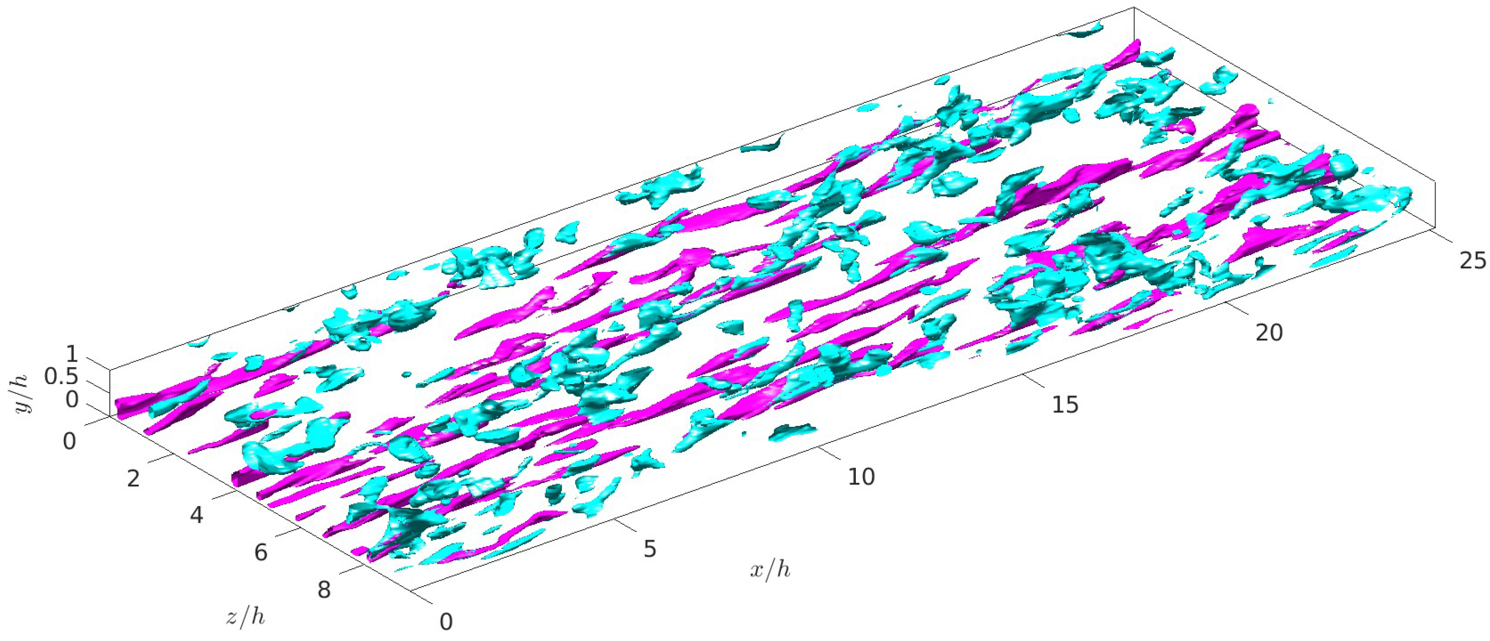
One obtains a Boolean field of the same size as the velocity after using any of these definitions, or any other, to obtain these coherent structures. This array contains a true value (1) if the point belongs to a structure or false (0) if not. The main point of this paper starts here. An algorithm is needed to obtain the individual structures. In Figure 1, several long high-velocity streaks (pink) are shown. These structures are very close to the wall, while Q-structures (light blue) are present across the whole channel.

One very important point in these problems is the aforementioned percolation index, i.e., the constant in Equations  (3) and (2). If these numbers are close to 0, a single structure with a porous shape appears. On the contrary, almost all structures are removed from the flow if the percolation index is too large. In the literature [38], the criteria for choosing a percolation index involve achieving a volume ratio below 10% while maintaining an object identification ratio close to unity. This approach ensures that the identified structures represent a sufficient population and are spaced adequately to yield reliable statistical outcomes. On the other hand, this requires a very demanding study where many different configurations must be tested.

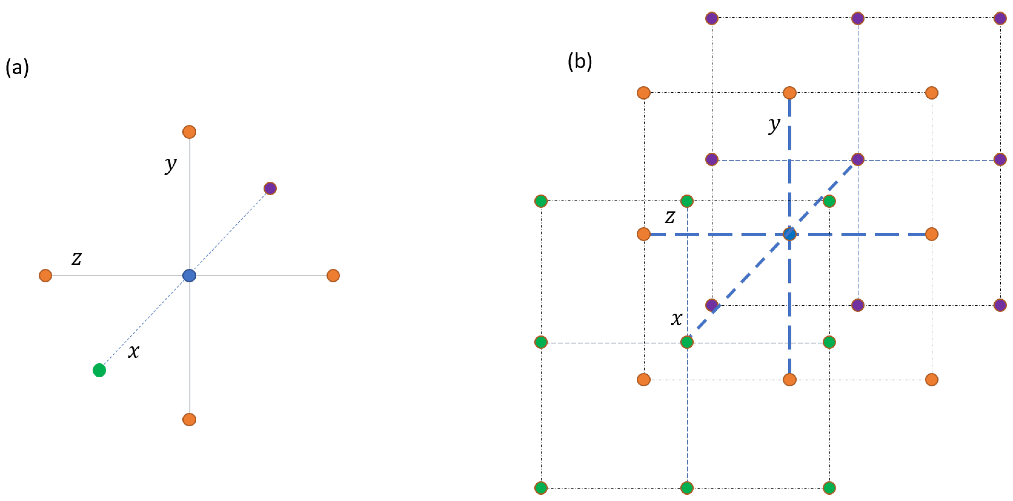
The first point in defining a structure is to decide the connections among the different points of the structure. Figure 2 summarizes the two alternatives. As turbulence is a 3D problem, this point has to be considered in the structure’s definition. Note that any other way of defining any coherent structure is also valid. Here, these two definitions are employed to show how the algorithm works for two different cases.

2.1. Direct Queue

In the first case, Figure 2a, two points belong to the same structure if a path joins them following only the three axes. Paths running through the diagonals are allowed for the 26-connectivity case, Figure 2b. In both cases, the results are similar. The second stencil produced fewer and a bit larger structures, but this effect happens almost entirely for the smallest structures.

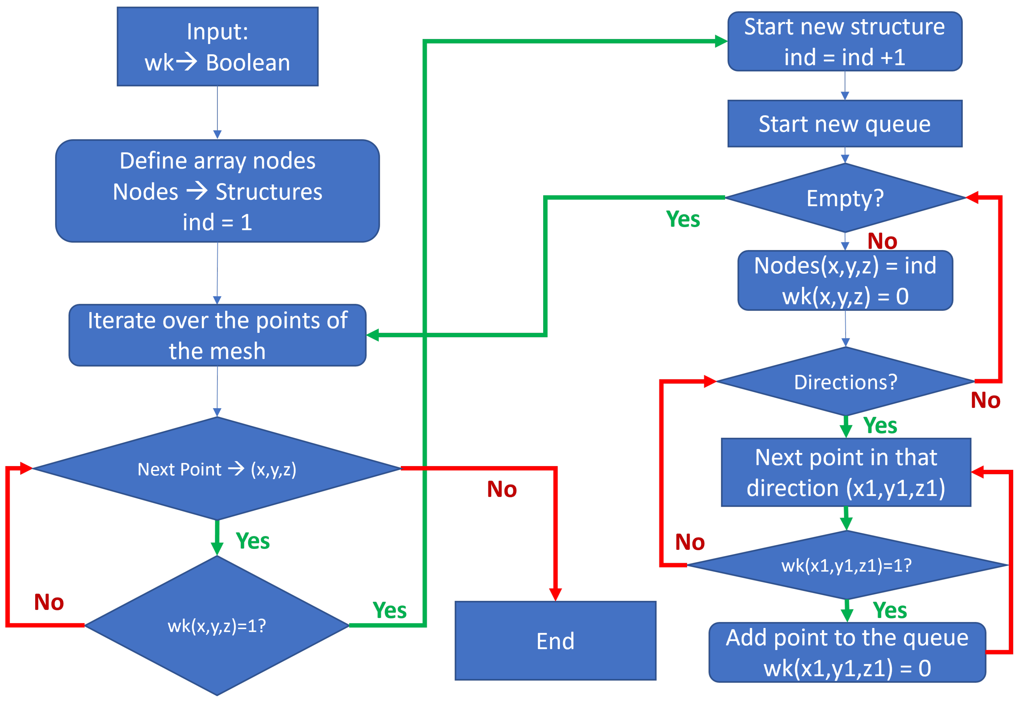
The main idea in both cases is illustrated in the flow diagram presented in Figure 3. The algorithm takes a Boolean array, $wk$, as input and produces an output array of the same size that stores the identified structures. The simplest way to organize the output is by replacing the true values with a unique identifier for each vortex. As will be shown later, this approach is easily parallelized. Moreover, identifying a specific structure can be done by simply reading one array in memory.

The code iterates over the mesh points. When a point with $wk(x,y,z)=1$ is found, the queue subalgorithm begins. A queue is created, with this point as the first entry. From there, the algorithm checks in every possible direction, adding points to the queue if $wk(x1,y1,z1)=1$, where $(x1,y1,z1)$ are the coordinates of the new point. The search in that direction stops once $wk(x1,y1,z1)=0$. To prevent adding the same point multiple times, $wk(x1,y1,z1)$ is set to 0 when the point is added to the queue.

Algorithm 1, 3D queue method describes the procedure to directly obtain the structures using these two stencils. The main points of this algorithm are:

• Lines 2–7. Define an array with the different directions one may follow. Six directions are needed for the first case, and twenty-six are needed for the second one.
• Lines 8–15. Initialize memory and start checking all points. If $wk$ is 0, the rest of the loop is skipped.
• Lines 16–20. This point is the starting point of a vortex. Initialize the queue and three indices:

  −

  $np$ is the length of the vortex;

  −

  $nq$ is the point to be studied;

  −

  $sq$ is the index of the points added to the queue.

• Line 20. The loop ends when all the points in the queue have been analyzed.
• Lines 20–35. Main loop:

  −

  Lines 21–22. Save this point in the structure register;

  −

  Line 24. Change the Boolean to 0. This 0 avoids working at this point again but seriously harms the chances of using openMP;

  −

  Lines 26–32. Follow every possible direction, adding points to the queue. The Boolean is set to zero after including the point.

Algorithm 1 3D queue method
1:	Input: Boolean matrix wk, dimensions nx, ny, nz, flag
2:	Output: Intenger matrix nodes, dimensions nx, ny, nz
3:	if flag == 1 then
4:	Define dirs as a $6\times 3$ matrix with the directions: $$\begin{array}{ccc}-1& 0& 0\\ 0& -1& 0\\ 0& 0& -1\\ 1& 0& 0\\ 0& 1& 0\\ 0& 0& 1\end{array}$$
5:	else
6:	Initialize dirs as a $26\times 3$ matrix containing every possible direction
7:	end if
8:	ldirs = size of the first dimension of dirs
9:	Initialize queue as a $3\times pdim$ integer array of zeros
10:	Initialize ind as 1
11:	for k = 2 to ny-1 do
12:	for j = 1 to nz do
13:	for i = 1 to nx do
14:	if wk(i, j, k) == 0 then
15:	continue
16:	end if
17:	Assign queue(:,1) = [i; j; k]
18:	Initialize np = 1
19:	Initialize nq = 1
20:	Initialize sq = 1
21:	while nq <= sq do
22:	Assign vrtini = queue(:, nq)
23:	Assign nodes(vrtini) = ind
24:	Increment np by 1
25:	Assign wk(vrtini(1), vrtini(2), vrtini(3)) = 0
26:	for ld = 1 to ldirs do
27:	Compute vrt based on dirs(ld,:) and vrtini
28:	while vrt(3) != -1 and wk(vrt(1), vrt(2), vrt(3)) == 1 do
29:	Increment sq by 1
30:	Assign queue(:,sq) = vrt
31:	Assign wk(vrt(1), vrt(2), vrt(3)) = 0
32:	Update vrt to the next position in the same direction
33:	end while
34:	end for
35:	Increment nq by 1
36:	end while
37:	Increment ind by 1
38:	end for
39:	end for
40:	end for

After this algorithm, one gets the entire structure of the fields. To analyze it, a second set of routines were produced, including, for example, one algorithm that saves this data as a structure array in Matlab (or their equivalent in any other language) with the following fields:

• pointsx: Array containing the x-coordinate;
• pointsy: Array containing the y-coordinate;
• pointsz: Array containing the z-coordinate;
• maxx: Maximum value of x;
• maxy: Maximum value of y;
• maxz: Maximum value of z;
• minx: Minimum value of x;
• miny: Minimum value of x;
• minz: Minimum value of x;
• nx: Problem size in x direction;
• ny: Problem size in y direction;
• nz: Problem size in z direction.

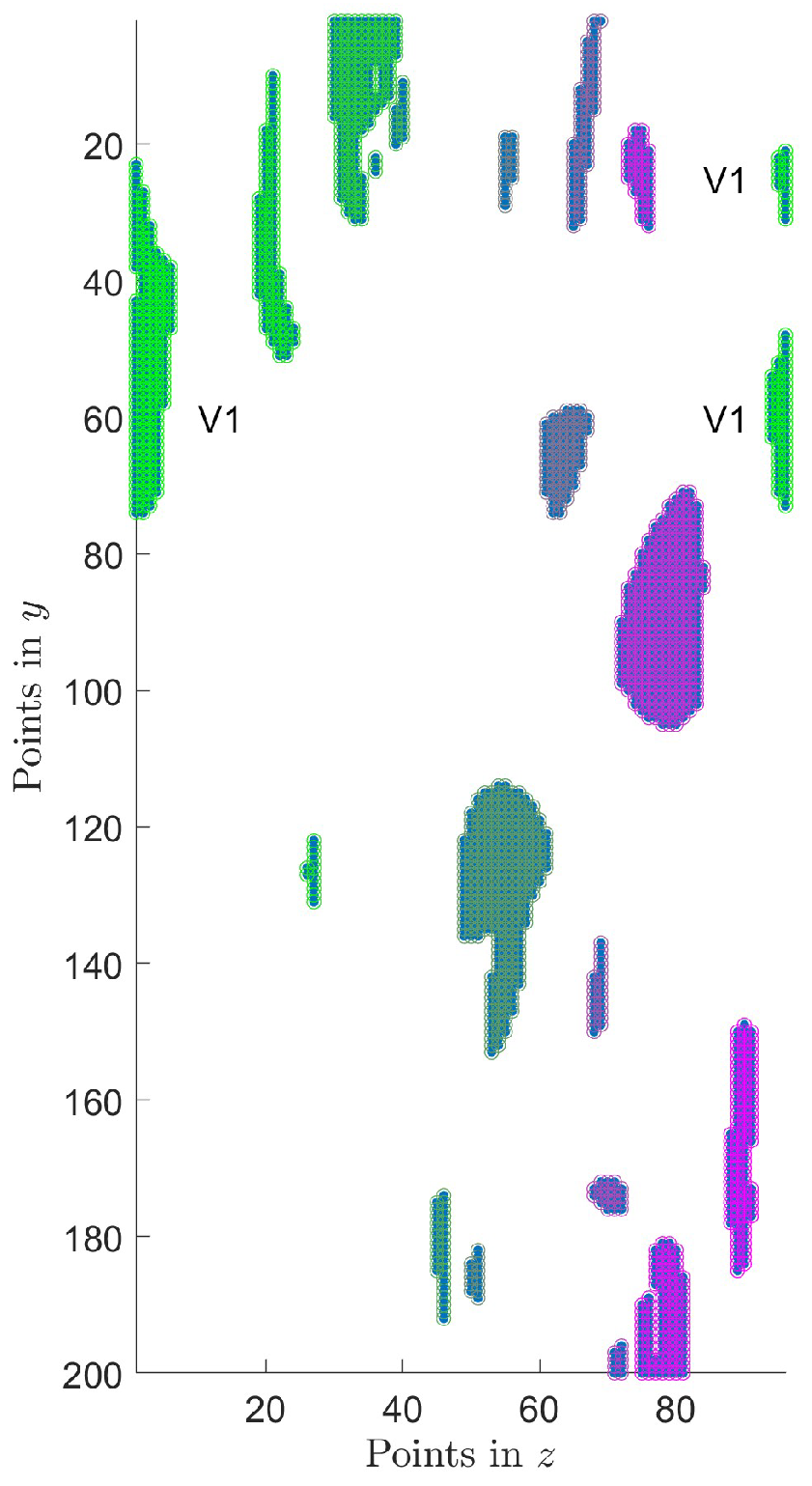
This algorithm does not account for the periodicity of the box in the x and z directions. A 2D example is shown in Figure 4. Creating a separate routine to merge these vortices is more efficient than incorporating the code directly into Algorithm 1. The z-direction version of this code is presented in Algorithm 2. This algorithm uses information stored in the structure, such as vortex(1).nz. Additionally, this algorithm is iterative, as new merges may occur after some structures have been combined.

This second algorithm has three very different parts:

• Lines 3–14. Identifies the structures that contain at least one point at the domain’s left or right boundaries;
• Lines 17–39. Check if, for the same value of y, there is a point in common for any left-right pair;
• Lines 40–47. The algorithm ends here if no structures to join are found (line 41). On the contrary, the structures are joined (line 44), the right ones are removed from the list, and the function is called again.

Algorithm 2 Check Vortex Periodicity in the z-Direction
1:	Input: Array of vortex structures vortex and its length n
2:	Output: Modified array of vortex structures with periodicity in z checked
3:	Initialize indl = 0
4:	Initialize indr = 0
5:	for ix = 1 to n do
6:	if vortex(ix).minz == 1 then
7:	indl = indl + 1
8:	left(indl) = ix
9:	end if
10:	if vortex(ix).maxz == vortex(ix).nz then
11:	indr = indr + 1
12:	right(indr) = ix
13:	end if
14:	end for
15:	Initialize join = 0
16:	Initialize ind = 1
17:	for ii = 1 to indl do
18:	pyl = vortex(left(ii)).pointsy
19:	pyz = vortex(left(ii)).pointsz
20:	I = find(pyz == 1)
21:	pyl = pyl(I)
22:	for jj = 1 to indr do
23:	if left(ii) == right(jj) then
24:	continue
25:	end if
26:	pyr = vortex(right(jj)).pointsy
27:	pyz = vortex(right(jj)).pointsz
28:	I = find(pyz == vortex(1).nz)
29:	pyr = pyr(I)
30:	isContained = any(ismember(pyl, pyr))
31:	if isContained then
32:	join = 1
33:	IL(ind) = left(ii)
34:	IR(ind) = right(jj)
35:	ind = ind + 1
36:	Print "join left(ii) and right(jj)"
37:	end if
38:	end for
39:	end for
40:	if join == 0 then return
41:	return
42:	end if
43:	for ii = 1 to ind - 1 do
44:	vortex(IL(ii)) = joinVortex(vortex(IL(ii)), vortex(IR(ii)))
45:	end for
46:	Remove vortex(IR) from the list
47:	Recursively call checkPeriodicityz(vortex)

2.2. A Parallel Algorithm

The previous algorithms were implemented sequentially because it is possible to add points to the structure in any direction. However, to tackle large problems, it is imperative to use parallel computing.

One initial approach would be to utilize shared memory libraries, with OpenMP being the most popular option [39]. In this framework, all processors have access to the entire memory. However, this is inappropriate in this case, as processor A can access $wk(x,y,z)$ and change its value to 0, which would stop the calculations of any other processor traversing that point. Unfortunately, this could also be true for GPU architectures, as OpenMP is somehow similar to them.

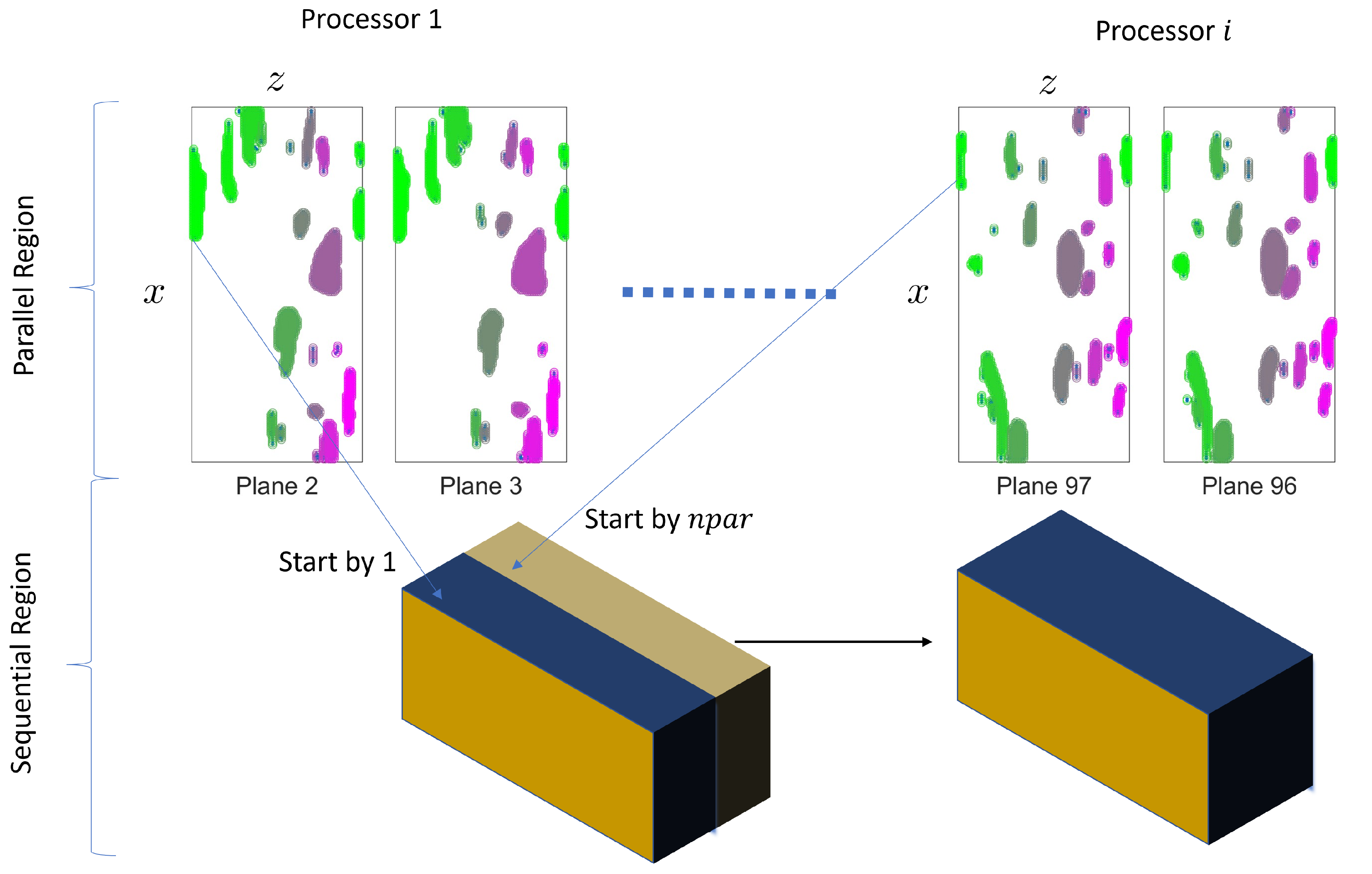
The proposed approach involves utilizing the Message Passing Interface (MPI) [40]. With MPI, each processor has access solely to its own memory, enabling efficient parallel computation. Data can be managed through the parallel input/output library HDF5 [41]. Consequently, segments of the entire array $wk$ can be distributed to each processor, as illustrated in Figure 5. The maximum number of processors, np, is the number of planes in y, which is typically large, avoiding memory problems. Each processor then uses Algorithm 1 to find their local structures and write them on disk.

The key point is that each processor starts numbering their structures using a large number, $npar$, that must be fixed arbitrarily. This situation is represented in the lower part of Figure 5, where two blocks come from two different processors. The blue one starts at 1 and the brown one at $npar$. One sequential algorithm, Algorithm 3, reads the intersection part and identifies the common structures, renumbering the ones of the second block. This procedure is very fast as it only needs reading two planes. The implementation chosen uses a recursive algorithm, as some disjoint structures of Processor 2 can be linked to the same structure of Processor 1. Thus, whenever two structures are identified (both are not zero at the same coordinates, and the index is not the same), the code stops searching and calls itself again.

Algorithm 3 Join Slices
1:	Input: Plane1, Plane2
2:	Output: Plane1, Plane2
3:	[nx, nz] = size(plane1)
4:	join = 0
5:	for kk = 1 to nz do
6:	for ii = 1 to nx do
7:	if (plane1(ii, kk) · plane2(ii, kk)≠ 0) and (plane1(ii, kk) - plane2(ii, kk)≠ 0) then
8:	ind1 = plane1(ii, kk)
9:	ind2 = plane2(ii, kk)
10:	plane2(plane2 == ind2) = ind1
11:	join = 1
12:	break
13:	end if
14:	end for
15:	if join = 1 then
16:	break
17:	end if
18:	end for
19:	if join = 1 then
20:	(plane1, plane2) = joinSlices(plane1, plane2)
21:	end if

3. Results

The data used in this section are outlined in Table 1, together with a reference to the paper in which they have been used. They were obtained as explained in the Methods section. The largest case, the P2k case, needs a memory of 60 GB if the Boolean is given. If this Boolean has to be included, the memory is close to 200 GB in the most favorable case. This number is 1.5 TB for the largest simulations today [9,10]. This code will be used in these huge fields in some future works. Several Reynolds numbers and meshes were used to consider the growing complexity of the problem. In every case, the resolution is adequate [35,42].

The main results of the algorithm are given in

Table 2. Absolute times in seconds. The first two columns result from the sequential algorithm for the 6D and 26D cases. The other columns correspond to 2, 4, 8, 16, and 32 processors, always for the 6D case.

Case	P1-6D	P1-26D	P2	P4	P8	P16	P32
P125S	0.03	0.08	0.0178	0.00855	0.00388	0.00166	0.00125
P125B	0.21	0.43	0.0875	0.0487	0.02461	0.00995	0.007368
P250	2.35	4.9	0.99	0.5	0.23	0.11	0.0774
P550	4.96	10.03	2.06	1.1	0.53	0.24	0.16
P1000	42.5	84.6	14.6	7.79	4.21	1.95	1.16

, including the times. The algorithm has been implemented in Fortran03. Two different computers were used. All cases up to P1000 included ran in an Intel(R) Xeon(R) CPU E5-2630 v4 @ 2.20 GHz with 128 GB of RAM. The P2000 case ran in three Intel Xeon Platinum 8174 Processor nodes, with 780 GB of RAM each.

The validation of the code has two parts. The first one accounts for the computation of the different physical magnitudes that define the structures. This validation was made for other works, particularly [3,27]. The second one involves the procedure from the Boolean to individual structures.

The first verification was made using several Booleans prepared ad hoc. Once the code was carefully checked, the first test was made it the data of the smallest case. In this case, it is very easy to see all the connections and check every result. In every case, the parallel algorithm gave exactly the same values as the sequential one. Not a single point was lost.

As shown in Table 2, the case Sequential 26 is slightly slower because there are more connections to follow. This very large computational stencil leads to a smaller number of structures, but they are far larger [36].

To further demonstrate the algorithm’s scaling and avoid working with dimensional quantities, the strong scaling of the algorithm has been computed. To do so, the time used in the sequential case is taken as a reference. All times are normalized using this value, and

Table 3. Performance results across different processor counts based on the results for the sequential case.

Case	P1	P2	P4	P8	P16	P32
P125S	1.00	2.12	4.42	9.74	22.77	30.24
P125B	1.00	2.40	4.31	8.53	21.11	28.50
P250	1.00	2.37	4.70	10.22	21.36	30.36
P550	1.00	2.33	4.35	9.04	19.96	29.94
P1000	1.00	2.91	5.46	10.10	21.79	36.64

is obtained. As can be seen, the values in this table are extremely close to the number of processors, indicating excellent strong scaling.

Finally, the case P2000 was tested on a different machine. The memory required for this case exceeds 200 GB, making it impossible to run the sequential algorithm. The results shown in

Table 4. Performance results for case P2000 across different processor counts.

Case	P16	P32	P64	P128
P2000 (Seconds)	12.75	5.34	2.18	0.88
P2000 (Scaling)	16.00	38.20	93.58	231.82

are excellent. Near-perfect strong scaling is exhibited by the algorithm. Furthermore, the overscaling is likely due to the smaller size of the local structures on each processor. Given the high scalability of the code, it can certainly be used to obtain the turbulent structures of a flow while the simulation is running.

4. Conclusions

This study has explored three different methods for identifying coherent structures within turbulent flows as they are simulated, thereby addressing a key obstacle in DNS: the immense data storage requirements. While effective for small-scale problems, sequential algorithms can not be used in large problems due to memory and time constraints.

The parallel algorithm proposed in this study offers a promising solution to this challenge. Leveraging multiple processors significantly accelerates the process of identifying and analyzing turbulent structures within large datasets. The algorithm has shown excellent strong scaling for small to large problems.

This parallel method improves computational efficiency and makes it feasible to handle the massive data generated by DNS, enabling more detailed and extensive studies of turbulence. In particular, the authors will continue using this algorithm to understand the problems in the accuracy of DNS and the dynamics of turbulent flows.