Leveraging Universal Adversarial Perturbation and Frequency Band Filters Against Face Recognition

Abstract

Universal adversarial perturbation (UAP) exhibits universality as it is independent of specific images. Although previous investigations have shown that the classification of natural images is susceptible to universal adversarial attacks, the impact of UAP on face recognition has not been fully investigated. Thus, in this paper we assess the vulnerability of face recognition for UAP. We propose FaUAP-FBF, which exploits the frequency domain by learning high, middle, and low band filters as an additional dimension of refining facial UAP. The facial UAP and filters are alternately and repeatedly learned from a training set. Furthermore, we convert non-target attacks to target attacks by customizing a target example, which is an out-of-distribution sample for a training set. Accordingly, non-target and target attacks form a uniform target attack. Finally, the variance of cosine similarity is incorporated into the adversarial loss, thereby enhancing the attacking capability. Extensive experiments on LFW and CASIA-WebFace datasets show that FaUAP-FBF has a higher fooling rate and better objective stealthiness metrics across the evaluated network structures compared to existing universal adversarial attacks, which confirms the effectiveness of the proposed FaUAP-FBF. Our results also imply that UAP poses a real threat for face recognition systems and should be taken seriously when face recognition systems are being designed.

1. Introduction

Deep neural networks (DNNs) play an increasingly vital role in processing large-scale data tasks, such as natural language processing [1], speech recognition [2], image classification [3], and face recognition [4]. Among them, face recognition serves as a powerful technique to confirm individual identity by analyzing facial features in the facial image. Currently, state-of-the-art face recognition methods primarily utilize DNNs to extract facial features to accomplish face recognition tasks. On the other hand, despite the significant progress of DNNs in a variety of tasks, they still suffer from security vulnerabilities. Attacks targeting DNNs, such as data poisoning [5], backdoor attacks [6], and adversarial attacks [7], have posed fatal threats to the integrity and reliability of DNNs. Adversarial attacks, in particular, were first discovered by Szegedy et al. [8]. By overlaying imperceptible and carefully crafted perturbations on input images, these attacks can lead to erroneous decisions from DNNs.

Generally, adversarial perturbations can be tailored specifically for each image and can also be learned using an image set sampled from an independent and identical distribution and used to contaminate any unseen image. The latter is known as universal adversarial perturbation (UAP). UAP was proposed by Moosavi-Dezfooli et al. [9] and can significantly diminish the neural network’s performance. Due to the generality of UAP, it has gained considerable attention in the task of natural image classification. Subsequent studies have proposed various approaches, including optimization-based and generative-network-based methods, to generate perturbations. In the face recognition realm, most adversarial attacks are image-specific, which means that perturbations are crafted for each facial image. For instance, in physical-world oriented face adversarial attacks [10], by generating a special kind of glasses around the eyes, the adversarial sample with the addition of the glasses is able to fool the face recognition network with a high probability. Adversarial attacks in the digital domain cheat face recognition models through iterative use of a small transparent patch on the face [11]. The approach proposed in [12] utilizes generative adversarial networks to produce adversarial samples with different makeup styles based on various face shapes to deceive the target model.

As a subset of image, and inspired by the success of UAP for natural images, we argue that UAP is feasible for fooling face recognition system. Unlike the natural image classification, however, facial image recognition belongs to fine-grained recognition. Thus, the proposed UAP regarding natural images is insufficient for facial images and needs refining to adapt to fine-grained cases. In addition, the existing UAP for natural images is generated from ether the spatial domain or the frequency domain rather than simultaneously considering both of the two domains. We believe the UAP designed covering both domains tends to have promising performance. To combine all the mentioned factors, we exploit the frequency domain as an additional dimension to refining perturbations produced from the spatial domain, namely Facial UAP and frequency band filters (FaUAP-FBFs). Concretely, in the frequency domain there exists a notable band region partition for the energy distribution of images where most of the energies concentrate on the low band and significantly attenuate in the middle and high bands. Furthermore, the band partition is directly connected to human visual perception; for instance, human vision is usually more sensitive to the low band. It prompts us to differentiate the importance and influence for perturbations in different bands, which can be implemented by learning different band filters. Under the general proposed framework, we also propose two innovative strategies. One innovative strategy is that we convert non-target attacks to target attacks by customizing a target example. In essence, the customized target example is an out-of-distribution sample for a training set. Hence, reducing the distance between the adversarial example and the customized example is aligned with out-of-distribution non-target attack. Also, by using the customized example, the attack is immune to the uncertain non-target victim. Accordingly, non-target and target attacks form a uniform target attack. The other innovative strategy is that, to enhance the attacking capacity, the distribution of cosine similarity between a batch of adversarial example and the target example is considered and the variance of the distribution is incorporated into the adversarial loss. This incorporation facilitates a more consistent alignment between the adversarial example and the target example.

The main contributions of this paper are summarized as follows:

• We assess the vulnerability of face recognition for UAP and exploit the frequency domain by learning high, middle, and low band filters as an additional dimension of refining facial UAP.
• We customize a target example to convert the non-target attack to a target attack. The customized example is an out-of–distribution sample for a training set. Accordingly, non-target and target attacks form a uniform target attack.
• We introduce variance of cosine similarity between a batch of adversarial examples and the target example into the adversarial loss. Reducing the variance contributes to aligning the adversarial example with the target example.

The organization of this paper is as follows: We briefly review related works in Section 2. In Section 3, we elaborate on the research motivation and the methodology for the proposed FaUAP-FBF. Then, we conduct extensive experiments and demonstrate the effectiveness of FaUAP-FBF in Section 4. Finally, we summarize the full paper and provide details of future work in Section 5.

2. Related Works

2.1. Background of Face Recognition

Face recognition is routinely divided into two sub-tasks: face verification [13], which determines whether a pair of facial images belong to the same person, and face identification [14], which identifies the person in a facial image. Generally, the current state-of-the-art face recognition systems use deep CNNs to extract feature representation from facial images, then the systems compute the distance between two feature representations, thereby quantifying the similarity between the two facial images. The similarity is ultimately utilized to accomplish face recognition. Network structure and loss of DNNs are two essential factors impacting the performance of face recognition. The more prevalent network structures are VGGNet [15], GoogLeNet [16], and ResNet [17]. For loss, Triplet loss [18], CosFace [19], and ArcFace [20] are well known and commonly used.

2.2. Adversarial Attacks on Face Recognition

As general attacks, existing attacks imposed on face recognition are also along the physical domain and the digital domain. Physical domain attacks endeavor to generate specialized wearable items or physical objects to deceive face recognition system. Sharif et al. [10] printed adversarial perturbations on eyeglass frames, which enables one to evade detection or impersonate others in face recognition. Komkov et al. [21] printed a rectangular strip of paper with a pattern and pasted it onto a hat, which does not cover the attacker’s facial features but still fools the face recognition system. Ibsen et al. [22] printed a special facial image onto a T-shirt that could confuse the face recognition system. Zheng et al. [23] explored sticker attacks by considering the complexity of environmental changes under different physical conditions. Digital domain attacks endeavor to generate digital perturbations to deceive face recognition systems. Dabouei et al. [24] modified the tiny spatial locations of the key points of the face and achieved a successful attack on the face recognition system. Dong et al. [25] proposed an evolutionary attack in a decision-based black-box scenario, which could characterize the geometrical structure of the decision boundary along the search direction and shrink the search space to improve the black-box attack efficiency. Hussain et al. [26] proposed a real-time attack based on an adversarial transfer network, where facial images could be fed into an adversarial transfer network to rapidly generate adversarial facial images for the purpose of real-time attacks.

2.3. Universal Adversarial Attacks on Image Classification

Universal adversarial attacks aim to use a single perturbation on any example to fool DNNs. Due to its convenience in one-generation and multiple use, this attack has attracted significant attentions from researchers. Moosavi-Dezfooli et al. [9] first demonstrated the existence of UAP for non-target attacks against CNNs on natural image classification tasks. Mopuri et al. [27] proposed the fast feature fool (FFF) algorithm, which generates universal adversarial perturbations without relying on data. Subsequent research connected UAP generation with generative adversarial networks (GANs). Hayes et al. [28] proposed the universal adversarial network, aimed at learning the distribution of perturbations rather than a single perturbation. Mopuri et al. [29] proposed a network for adversary generation (NAG) to create adversarial perturbations for a given CNN classifier. This network utilizes the attributions of examples to model the distribution of adversarial perturbations and achieves effectiveness and diversity in perturbation generation thereafter. Zhang et al. [30] offer a new perspective on the relationship between carrier image and UAP. They suggest that perturbations hold key features dominating model decisions, which enables the carrier image to be treated as noise. Based on this idea, they designed a feature-dominant algorithm allowing the use of external data for both target and non-target universal attacks. Building upon UAP, Deng et al. [31] proposed generating UAP for texture images in the frequency domain by limiting the intensity of the perturbation using an JND model in the frequency domain. Sun et al. [32] explored universal adversarial attacks on vision transformers. Zolfi et al. [33] proposed a universal adversarial mask that could be used in the real world, but it was useless, however, under a surveillance setting. Duan et al. [34] utilized the common gradient of the perturbations of multiple face images to optimize universal adversarial perturbation, and dominant feature loss was proposed to improve the attack capability of the perturbation. Qiao et al. [35] exploited universal adversarial perturbation as a watermark to defend against facial forgery across a wide range of forgery methods.

Most of the existing adversarial attacks against face recognition focus on image-specific perturbation. This paper follows the approach of universal adversarial attacks, aiming to generate universal perturbation that can deceive facial images across the entire dataset, namely, image-agnostic perturbation.

3. Proposed Method

3.1. Refining UAP in Frequency Domain via Learnable Filters

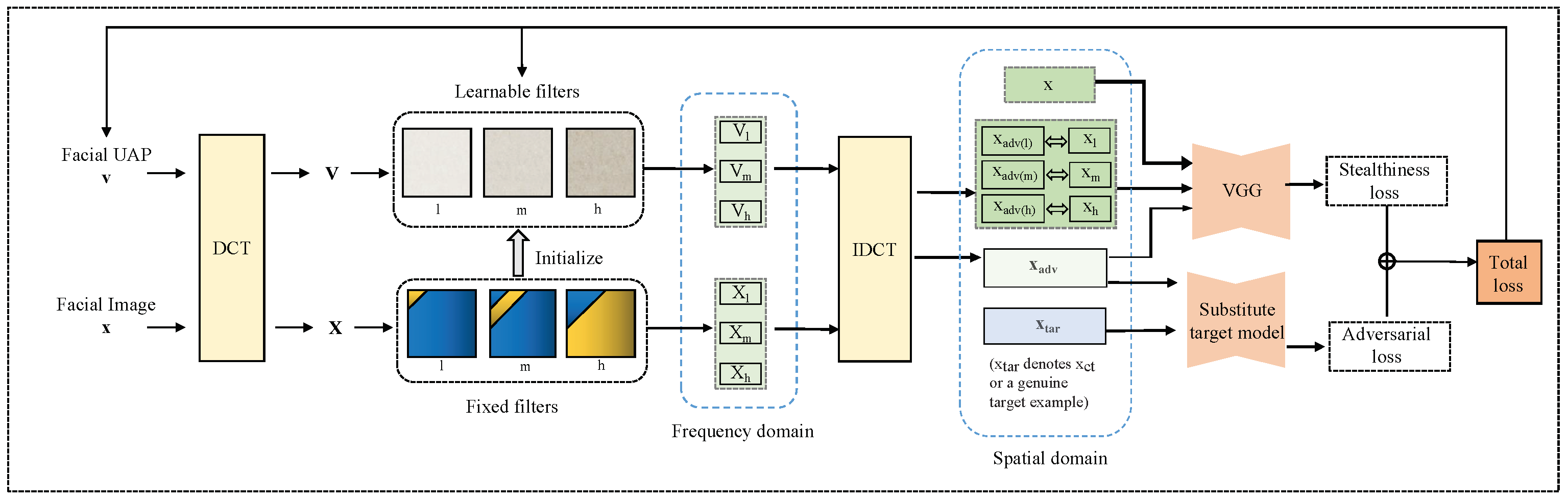
For a general understanding of our idea, we here outline the general procedure of FaUAP-FBF, as shown in Figure 1. The lowercase letters and capital letters denote examples in the spatial domain and frequency domain, respectively. The two domains are mutually converted by using discrete cosine transform (DCT) and inverse discrete cosine transform (IDCT). For the images, DCT is used to transform an image block from the spatial domain to the frequency domain, and IDCT is used to reconstruct an image block from the frequency domain to the spatial domain. Suppose there is a matrix $\mathbf{A}\in {\mathbb{R}}^{n\times n}$, where $a_{i,j}$ represents the element at position $(i,j)$; after DCT transformation, we obtain the transformed matrix $\mathbf{B}\in {\mathbb{R}}^{n\times n}$, where the element $b_{i,j}$ at position $(i,j)$ can be expressed as:

$$b_{i,j}=c_i{c}_j\sum _{p=0}^{n-1}\sum _{q=0}^{n-1}{a}_{p,q}cos\left({\displaystyle \frac{(2p+1)i\pi }{2n}}\right)cos\left({\displaystyle \frac{(2q+1)j\pi }{2n}}\right),$$

where $c_i=c_j=1/\sqrt{4n}$ for $i=j=0$ and $c_i=c_j=1/\sqrt{2n}$ otherwise. $\mathbf{A}$ can be reconstructed from $\mathbf{B}$ by using IDCT, i.e.,

$$a_{i,j}=\sum _{p=0}^{n-1}\sum _{q=0}^{n-1}{c}_p{c}_q{b}_{p,q}cos\left({\displaystyle \frac{(2i+1)p\pi }{2n}}\right)cos\left({\displaystyle \frac{(2j+1)q\pi }{2n}}\right).$$

For an 8 × 8 spatial block, DCT encapsulates 64 distinct frequency components. We employ the widely used Type-II DCT for both DCT and IDCT.

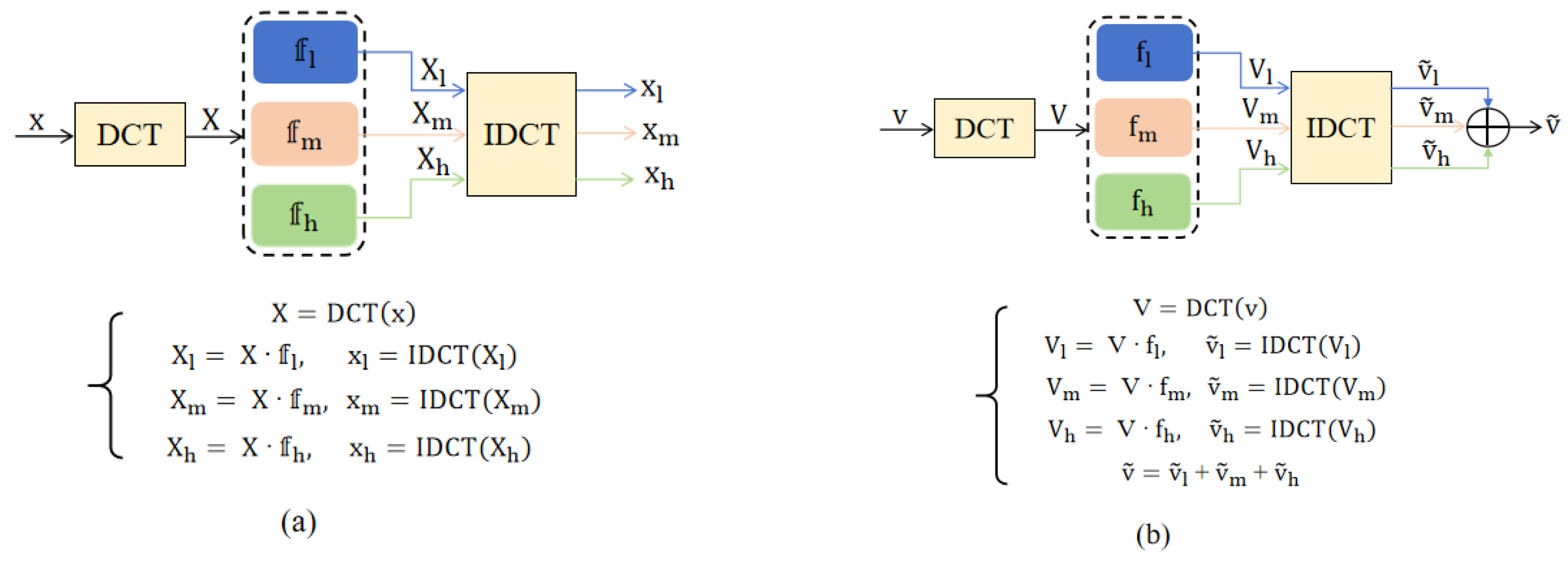
The filters used in FaUAP-FBF consist of fixed filters and learnable filters in high, middle, and low frequency bands, in which the fixed filters are used to separate the legitimate example into non-overlapped three frequency regions, and learnable filters are used to refine the perturbation using three band filters. Details for frequency domain filtering using fixed filters and learnable filters are shown in Figure 2a,b. {${𝕗}_{\mathrm{l}}$, ${𝕗}_{\mathrm{m}}$, ${𝕗}_{\mathrm{h}}$} and {${\mathrm{f}}_{\mathrm{l}}$, ${\mathrm{f}}_{\mathrm{m}}$, ${\mathrm{f}}_{\mathrm{h}}$} denote the fixed filters and learnable filters, respectively. For the fixed filters, the low-, middle-, and high-frequency bands account for hard separated regions in the entire spectrum, respectively, where each band region is sketched by a yellow color, and the values in the corresponding spectrum are set to 1, or 0 for the fixed filters. Further, they are used to initialize the learnable filters, and the ultimate values in the learnable filters are located in between 0 and 1. The fixed filters and learnable filters are shown in Figure 1 and  Figure 2.

First, both UAP and legitimate images in a training set are converted to the frequency domain through DCT, in which UAP in the spatial domain is initialized with Gaussian noise and the three learnable band filters are initialized with fixed filters. To calculate loss, both image and perturbation need to be converted back into the spatial domain through IDCT. During learning, both UAP in the spatial domain and the learnable filters are alternately and repeatedly updated in terms of a weighted combination of adversarial loss and stealthiness loss, and UAP in the spatial domain is also constrained by $l_{\infty }$-norm. The iteration continues until a certain criterion is satisfied. The target function is formulated as follows:

$$(\widehat{\mathrm{v}},{\widehat{\mathrm{f}}}_{\mathrm{l}},{\widehat{\mathrm{f}}}_{\mathrm{m}},{\widehat{\mathrm{f}}}_{\mathrm{h}})=\arg \underset{\mathrm{v},{\mathrm{f}}_{\mathrm{l}},{\mathrm{f}}_{\mathrm{m}},{\mathrm{f}}_{\mathrm{h}}}{min}\left[{\mathbb{E}}_{{\mathrm{x}}_{\mathrm{tr}}\sim \mathrm{D}}\left[{\mathcal{L}}_{\mathrm{adv}}\left({\mathrm{x}}_{\mathrm{adv}\left(\mathrm{tr}\right)},{\mathrm{x}}_{\mathrm{tar}}\right)+\lambda {\mathcal{L}}_{\mathrm{ste}}\left({\mathrm{x}}_{\mathrm{adv}\left(\mathrm{tr}\right)},{\mathrm{x}}_{\mathrm{tr}}\right)\right]\right]\mathrm{s}.\mathrm{t}.{∥\mathrm{v}∥}_{\infty }\le \xi$$

(1)

$${\mathrm{x}}_{\mathrm{adv}\left(\mathrm{tr}\right)}={\mathrm{x}}_{\mathrm{tr}}+\tilde{\mathrm{v}}$$

(2)

$${\mathrm{x}}_{\mathrm{adv}\left(\mathrm{tr}\right)}^{\left(\mathrm{s}\right)}={\mathrm{x}}_{\mathrm{tr}}^{\left(\mathrm{s}\right)}+{\tilde{\mathrm{v}}}_{\mathrm{s}},\mathrm{s}=\mathrm{l},\mathrm{m},\mathrm{h}$$

(3)

where ${\mathcal{L}}_{\mathrm{adv}}$ and ${\mathcal{L}}_{\mathrm{ste}}$ denote the adversarial loss and stealthiness loss, respectively, and $\lambda$ controls the balance between them. $\widehat{\mathrm{v}}$ and $\left\{\widehat{{\mathrm{f}}_{\mathrm{l}}},\widehat{{\mathrm{f}}_{\mathrm{m}}},\widehat{{\mathrm{f}}_{\mathrm{h}}}\right\}$ denote the optimal UAP and filters. ${\mathrm{x}}_{\mathrm{tar}}$ may be the customized target example or a genuine target example, and $\xi$ is a parameter controlling the strength of the perturbation. ${\mathrm{x}}_{\mathrm{tr}}$ and ${\mathrm{x}}_{\mathrm{adv}\left(\mathrm{tr}\right)}$ denote the legitimate training example and the corresponding adversarial example, and they are related with Equation (2). From Figure 1, it can be seen that, in addition to the whole example in the spatial domain, respective bands of the example in the spatial domain are also needed to calculate stealthiness loss. The respective bands of the example in the spatial domain are obtained using Equation (3). The calculations of $\tilde{\mathrm{v}}$ and $\{{\tilde{\mathrm{v}}}_{\mathrm{l}},{\tilde{\mathrm{v}}}_{\mathrm{m}},{\tilde{\mathrm{v}}}_{\mathrm{h}}\}$ are shown in Figure 2b.

Once $\widehat{\mathrm{v}}$ and $\left\{\widehat{{\mathrm{f}}_{\mathrm{l}}},\widehat{{\mathrm{f}}_{\mathrm{m}}},\widehat{{\mathrm{f}}_{\mathrm{h}}}\right\}$ are obtained, they can be utilized to yield an adversarial example for a legitimate test example, as explained in Equation (4):

$${\mathrm{x}}_{\mathrm{adv}\left(\mathrm{te}\right)}={\mathrm{x}}_{\mathrm{te}}+\mathrm{IDCT}\left[\mathrm{DCT}\left(\widehat{\mathrm{v}}\right)·\sum \widehat{{\mathrm{f}}_{\mathrm{s}}}\right],\mathrm{s}=\mathrm{l},\mathrm{m},\mathrm{h}$$

(4)

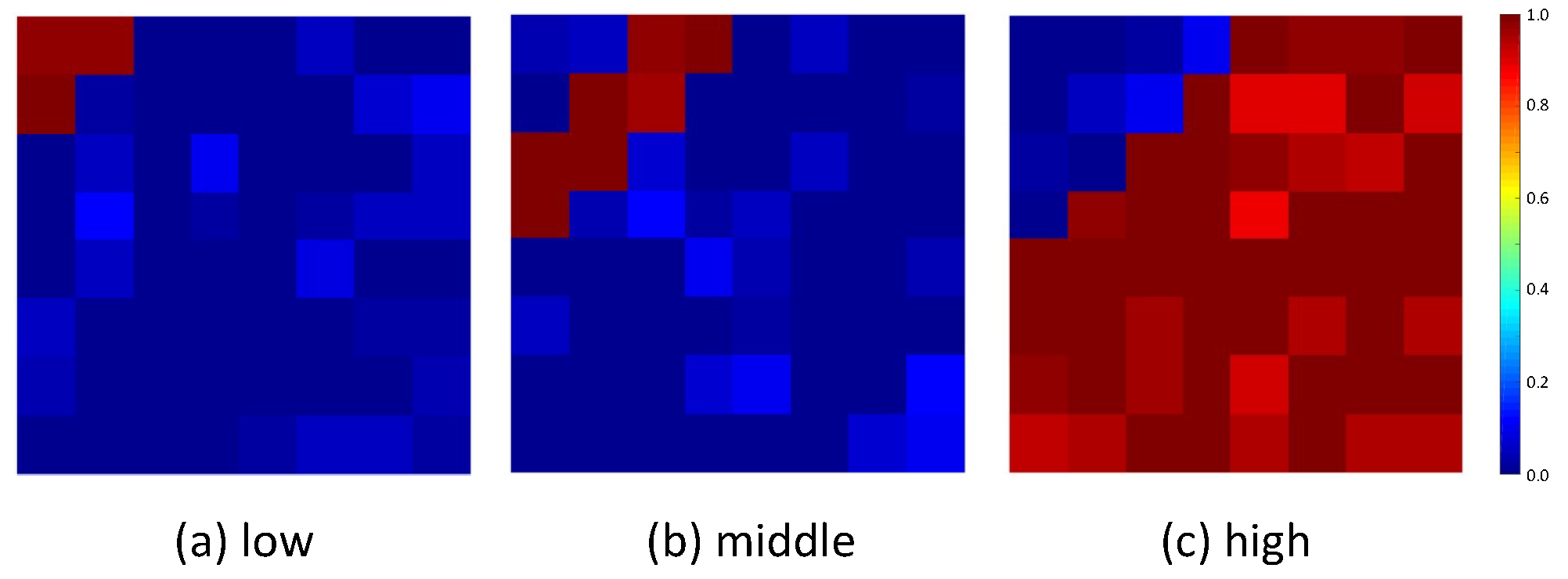
We apply the frequency domain as an additional dimension to iteratively optimize universal adversarial perturbations, allowing the optimizer to continually refine the perturbation to achieve the objective of fooling face recognition systems. The use of learnable filters ensures that the extracted frequency segment is not solely confined to the predefined high, middle-, and low-frequency ranges. Incorporating these adjustable filters facilitates the capture of subtle yet valuable information within each frequency segment. Consequently, this approach aligns the generated perturbation more closely with the frequency-divided facial image. The visualization of ultimately learned filters $\left\{\widehat{{\mathrm{f}}_{\mathrm{s}}},\mathrm{s}=\mathrm{l},\mathrm{m},\mathrm{h}\right\}$ are shown in Figure 3. The pipeline of FaUAP-FBF is provided in Algorithm 1, and the definitions of the notations used in this paper are listed in

Table 1. Definitions of used notations.

Notation	Definition
v, V	spatial domain/frequency domain perturbation
x, X	spatial domain/frequency domain legitimate example
${\mathrm{V}}_{\mathrm{l}}$, ${\mathrm{V}}_{\mathrm{m}}$, ${\mathrm{V}}_{\mathrm{h}}$	low/middle/high frequency component of perturbation
${\mathrm{X}}_{\mathrm{l}}$, ${\mathrm{X}}_{\mathrm{m}}$, ${\mathrm{X}}_{\mathrm{h}}$	low/middle/high frequency component of legitimate example
${𝕗}_{\mathrm{l}}$, ${𝕗}_{\mathrm{m}}$, ${𝕗}_{\mathrm{h}}$	low/middle/high frequency band for fixed filter
${\mathrm{f}}_{\mathrm{l}}$, ${\mathrm{f}}_{\mathrm{m}}$, ${\mathrm{f}}_{\mathrm{h}}$	low/middle/high frequency band for learnable filter
${\mathrm{x}}_{\mathrm{tr}}$, ${\mathrm{x}}_{\mathrm{adv}\left(\mathrm{tr}\right)}$	spatial domain legitimate example/adversarial example in training set
${\mathrm{x}}_{\mathrm{te}}$, ${\mathrm{x}}_{\mathrm{adv}\left(\mathrm{te}\right)}$	spatial domain legitimate example/adversarial example in test set
${\mathrm{x}}_{\mathrm{tr}}^{\left(\mathrm{l}\right)}$, ${\mathrm{x}}_{\mathrm{tr}}^{\left(\mathrm{m}\right)}$, ${\mathrm{x}}_{\mathrm{tr}}^{\left(\mathrm{h}\right)}$	low/middle/high frequency component in spatial domain legitimate example in training set
${\mathrm{x}}_{\mathrm{adv}\left(\mathrm{tr}\right)}^{\left(\mathrm{l}\right)}$, ${\mathrm{x}}_{\mathrm{adv}\left(\mathrm{tr}\right)}^{\left(\mathrm{m}\right)}$, ${\mathrm{x}}_{\mathrm{adv}\left(\mathrm{tr}\right)}^{\left(\mathrm{h}\right)}$	low/middle/high frequency component in spatial domain adversarial example in training set
${\mathrm{x}}_{\mathrm{tar}}$, ${\mathrm{x}}_{\mathrm{ct}}$	spatial domain target example/customized target example

.

Algorithm 1 The procedure of FaUAP-FBF

Input: Training set $\mathrm{D}$, ${\mathrm{x}}_{\mathrm{tar}}$ (customized target example ${\mathrm{x}}_{\mathrm{ct}}$ or a genuine target example), substitute target model $\mathrm{F}(·)$, fooling rate $\delta$, $l_{\infty }$ norm restriction of perturbation $\xi$, fixed filters $\{{𝕗}_{\mathrm{s}},\mathrm{s}=\mathrm{l},\mathrm{m},\mathrm{h}\}$ and decision threshold t, learning rate $\eta$. Output: Universal adversarial perturbations $\mathrm{v}$ and learnable filters $\{{\mathrm{f}}_{\mathrm{s}},\mathrm{s}=\mathrm{l},\mathrm{m},\mathrm{h}\}$ 1: Initialize $\mathrm{v}\leftarrow \mathrm{Gaussian}\mathrm{noise},\left\{{\mathrm{f}}_{\mathrm{s}}\right\}\leftarrow \left\{{𝕗}_{\mathrm{s}}\right\}$ 2: while $\mathrm{FR}<\delta$ do 3:     for a batch of examples $\left\{{\mathrm{x}}_i\right\}$ in $\mathrm{D}$ do 4:         Perform DCT transformation to obtain $\left\{{\mathrm{X}}_i\right\}$; use $\left\{{𝕗}_{\mathrm{s}}\right\}$ to obtain $\left\{{\mathrm{X}}_{\mathrm{s}}^{\left(i\right)}\right\}$ 5:         Perform DCT transformation to obtain $\mathrm{V}$; use $\left\{{\mathrm{f}}_{\mathrm{s}}\right\}$ to obtain ${\mathrm{V}}_{\mathrm{s}}$ 6:         Perform IDCT transformation to obtain $\left\{{\mathrm{x}}_{\mathrm{adv}}^{\left(i\right)}\right\}=\left\{{\mathrm{x}}_i\right\}+IDCT\left(\mathrm{V}·\sum {\mathrm{f}}_{\mathrm{s}}\right),\mathrm{s}=\mathrm{l},\mathrm{m},\mathrm{h}$ 7:         if average $\mathrm{Similarity}\left\{\left(\mathrm{F}\left({\mathrm{x}}_{\mathrm{adv}}^{\left(i\right)}\right),\mathrm{F}\left({\mathrm{x}}_i\right)\right)\right\}>t$ or average $\mathrm{Similarity}\left\{\left(\mathrm{F}\left({\mathrm{x}}_{\mathrm{adv}}^{\left(i\right)}\right),\mathrm{F}\left({\mathrm{x}}_{\mathrm{tar}}\right)\right)\right\}<t$ then 8:            $(\Delta \mathrm{v},\Delta \left\{{\mathrm{f}}_{\mathrm{s}}\right\})\leftarrow -\eta {\nabla }_{\mathrm{v},\left\{{\mathrm{f}}_{\mathrm{s}}\right\}}{\mathcal{L}}_{\mathrm{all}}$ 9:            Update the learnable filters $\left\{{\mathrm{f}}_{\mathrm{s}}\right\}\leftarrow \left\{{\mathrm{f}}_{\mathrm{s}}\right\}+\Delta \left\{{\mathrm{f}}_{\mathrm{s}}\right\}$ 10:             Update the perturbation $\mathrm{v}\leftarrow \mathrm{v}+\Delta \mathrm{v}$ 11:             Clip $\mathrm{v}$ to satisfy the $l_{\infty }$ norm restriction $\xi$ 12:             Update $\mathrm{V}$, ${\mathrm{V}}_{\mathrm{s}}$, $\left\{{\mathrm{x}}_{\mathrm{adv}}^{\left(i\right)}\right\}$ 13:         end if 14:     end for 15: end while 16: return $\mathrm{v}$ and $\left\{{\mathrm{f}}_{\mathrm{s}}\right\}$

We abstract seven computation units and summarize the overall and dominant time required for FaUAP-FBF by using the seven computation units and parameters of the training set and the hyper-parameters of the learning algorithm. These are listed in

Table 2. Computation Analysis for FaUAP-FBF during training.

Forward		Backward
legitimate image set	adversarial image set	filters
$\mathrm{N}\times \mathrm{M}\times \left({\mathrm{T}}_{\mathrm{DCT}}+3\times \left({\mathrm{T}}_{\mathrm{IDCT}}+{\mathrm{T}}_{\mathrm{filt}}\right)\right)+\left(\mathrm{N}\times 4\times {\mathrm{T}}_{\mathrm{VGG}}\right)$	$\mathrm{l}\times \mathrm{N}/\mathrm{n}\times \mathrm{N}\times \left(4\times {\mathrm{T}}_{\mathrm{VGG}}+{\mathrm{T}}_{\mathrm{tar}}\right)$	$\mathrm{l}\times \mathrm{N}/\mathrm{n}\times 3\times {\mathrm{T}}_{\mathrm{grad}\mathrm{for}\mathrm{f}\in {\mathrm{R}}^{3\times 3}}$
perturbation		perturbation
$\mathrm{l}\times \mathrm{N}/\mathrm{n}\times \mathrm{M}\times \left({\mathrm{T}}_{\mathrm{DCT}}+3\times \left({\mathrm{T}}_{\mathrm{IDCT}}+{\mathrm{T}}_{\mathrm{filt}}\right)\right)$		$\mathrm{l}\times \mathrm{N}/\mathrm{n}\times {\mathrm{T}}_{\mathrm{grad}\mathrm{for}\mathrm{v}\in {\mathrm{R}}^{\mathrm{p}\times \mathrm{q}}}$

. Specifically, there are two phases of forward and backward computation. In forward computation, there are five computation units, including DCT, IDCT, filtering, and feature extraction from VGG and from the substitute target model, in which the consumed time of the five computation units are denoted as ${\mathrm{T}}_{\mathrm{DCT}},{\mathrm{T}}_{\mathrm{IDCT}},{\mathrm{T}}_{\mathrm{filt}},{\mathrm{T}}_{\mathrm{VGG}},$ and ${\mathrm{T}}_{\mathrm{tar}}$, respectively. In backward computation, there are two computation units, including filter gradient computation and perturbation gradient computation, in which the times consumed for the two computation units are denoted as ${\mathrm{T}}_{\mathrm{grad}\mathrm{for}\mathrm{f}\in {\mathrm{R}}^{3\times 3}}$ and ${\mathrm{T}}_{\mathrm{grad}\mathrm{for}\mathrm{v}\in {\mathrm{R}}^{\mathrm{p}\times \mathrm{q}}}$, respectively. Here, $\mathrm{p}$ and $\mathrm{q}$ denote the width and height of UAP. $\mathrm{N}$ and $\mathrm{M}$ denote the number of training examples and the number of blocks in size $8\times 8$. $\mathrm{l}$ and $\mathrm{n}$ are the learning iteration number and batch size. Notice that in forward computation, the legitimate image set computation only needs one time and is completed before iteration for learning the UAP and filters.

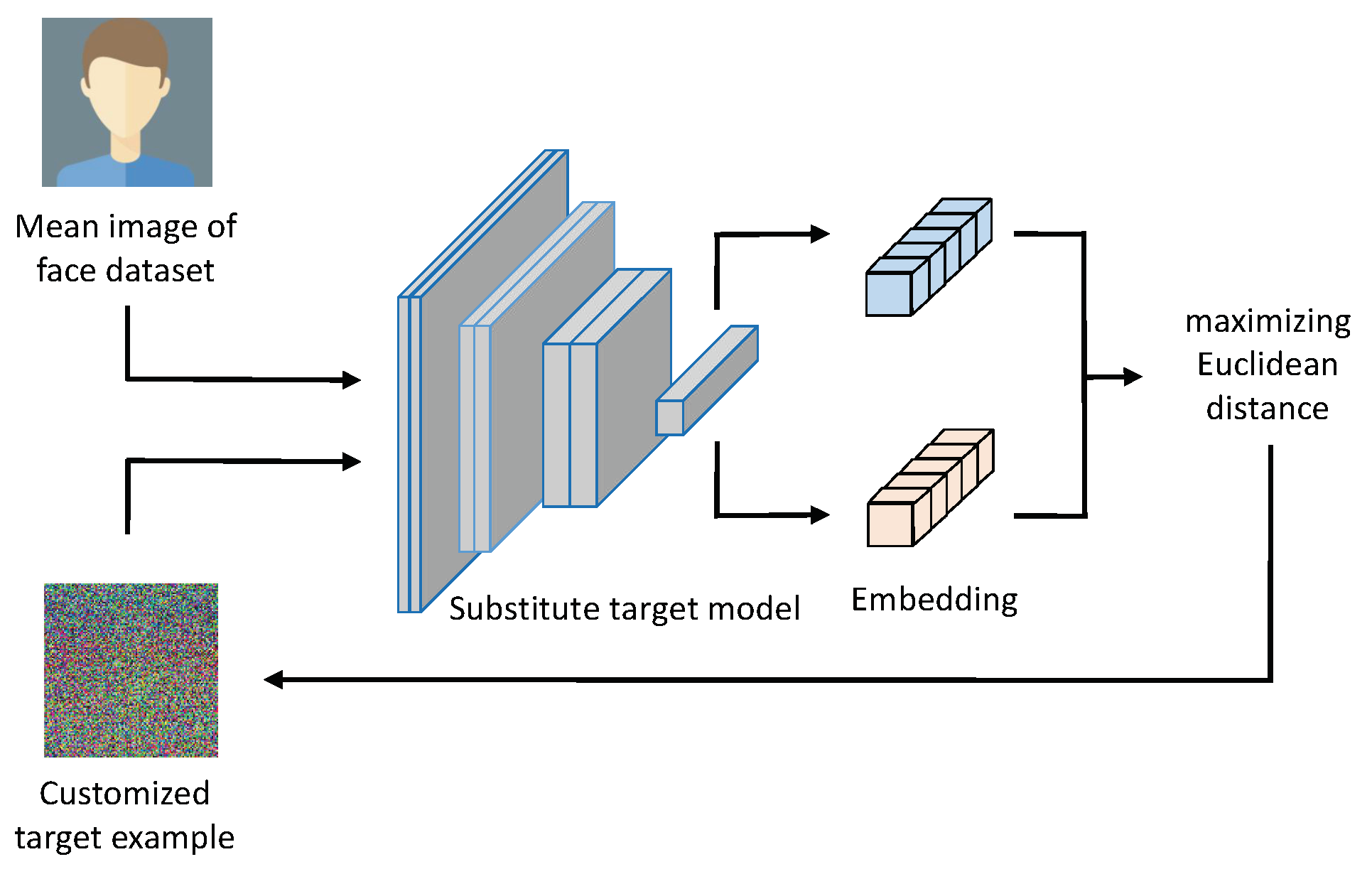
3.2. Non-Target Attack via Customizing a Target Example

Unlike the conventional non-target attack that forces the adversarial example to be away from an image of the specified person, we convert the non-target attack to be specific to varying victims to a unique target attack by customizing an example that is utilized as the target. Specifically, a customized target example ${\mathrm{x}}_{\mathrm{ct}}$ is sought by maximizing its distance from the overall distribution of the legitimate dataset. The flowchart is shown in Figure 4.

First, an image subset $\left\{{\mathrm{x}}_i,i=1,2,\cdots n\right\}$ is selected from legitimate dataset $\mathrm{D}$, which contains one facial image for each identity, and their average yields a mean image ${\mathrm{x}}_{\mathrm{o}}$ associated with the face dataset:

$${\mathrm{x}}_{\mathrm{o}}={\displaystyle \frac{1}{n}}\sum _{i=1}^n{\mathrm{x}}_i,{\mathrm{x}}_i\sim \mathrm{D}.$$

(5)

Subsequently, ${\mathrm{x}}_{\mathrm{ct}}$ is initialized by Gaussian noise and iteratively updated by progressively increasing the Euclidean distance between the embedding of ${\mathrm{x}}_{\mathrm{ct}}$ and ${\mathrm{x}}_{\mathrm{o}}$, in which the embeddings $\mathrm{F}\left({\mathrm{x}}_{\mathrm{ct}}\right)$ and $\mathrm{F}\left({\mathrm{x}}_{\mathrm{o}}\right)$ are extracted from the substitute target model (Arcface model). The procedure leads to ${\widehat{\mathrm{x}}}_{\mathrm{ct}}$, which significantly deviates from the distribution of the legitimate dataset, serving as our customized target example. It can be formulated as follows:

$${\widehat{\mathrm{x}}}_{\mathrm{ct}}=\arg \underset{{\mathrm{x}}_{\mathrm{ct}}}{max}{∥\mathrm{F}\left({\mathrm{x}}_{\mathrm{ct}}\right),\mathrm{F}\left({\mathrm{x}}_{\mathrm{o}}\right)∥}_2$$

(6)

where $\mathrm{F}$ refers to the substitute target model and $\mathrm{F}(·)$ denotes the embedding of the input image.

Since ${\widehat{\mathrm{x}}}_{\mathrm{ct}}$ has a significant distinction from the average of the legitimate dataset, decreasing the distance between the adversarial example and ${\widehat{\mathrm{x}}}_{\mathrm{ct}}$ is consistent with increasing the distance between the adversarial example and the image of an uncertain victim, thus achieving the desired effect of a non-target attack immune to specific non-target victims. Under a genuine target attack, the only necessary alteration is to replace the customized target example with the image of the desired victim, thereby unifying the non-target and target attack into a uniform target attack.

3.3. Loss Setting

3.3.1. Stealthiness Loss

The role of stealthiness loss is to control the visual concealment of the adversarial perturbation. We utilize the VGG (visual geometry group) network [15] to assess the stealthiness loss. VGG involves stacking multiple convolutional and pooling layers to extract hierarchical feature maps from images. VGG utilizes universal convolutional kernels and a layer hierarchy to increase the network’s depth. In particular, we use VGG 19 in our framework. VGG 19 includes 16 convolution plus ReLU layers, 5 max pooling layers, and 3 fully-connected plus ReLU layers, and all convolution kernels are $3\times 3$ in size. The shallow layers primarily focus on extracting low-level features such as edges, textures, and colors, which are sensitive to the local structures and fine details present in images. The subsequent deeper layers extract more advanced semantic features and higher-level features that possess the capability of capturing the abstract and global information present in images, enabling the network to recognize semantic objects in a more holistic manner. For stealthiness loss, low-level information such as texture is more likely to be noticed by the human eye and more aligned with the image quality assessment; thus, we use the feature maps given by the shallow layer of the VGG network to assess the stealthiness of the perturbations, as described in Equation (7):

$$\begin{array}{c}\hfill {\mathcal{L}}_{\mathrm{ste}}={\mathbb{E}}_{{\mathrm{x}}_{\mathrm{tr}}\sim \mathrm{D}}\left\{{∥{\phi }_j\left({\mathrm{x}}_{\mathrm{tr}}\right),{\phi }_j\left({\mathrm{x}}_{\mathrm{adv}\left(\mathrm{tr}\right)}\right)∥}_2+\sum _{\mathrm{s}=\mathrm{l},\mathrm{m},\mathrm{h}}{∥{\phi }_j\left({\mathrm{x}}_{\mathrm{tr}}^{\left(\mathrm{s}\right)}\right),{\phi }_j\left({\mathrm{x}}_{\mathrm{adv}\left(\mathrm{tr}\right)}^{\left(\mathrm{s}\right)}\right)∥}_2\right\}\end{array}$$

(7)

where ${\mathcal{L}}_{\mathrm{ste}}$ contains two parts; the first part evaluates the discrepancy between the whole legitimate example and the whole adversarial example, and the second part evaluates the discrepancy between them in the low-, middle-, and high-frequency bands, respectively, and ${\phi }_j$ is the feature map of the jth layer of the VGG network. We employ the ninth layer in our experiment.

3.3.2. Adversarial Loss

The role of adversarial loss is to control the attacking performance of the adversarial perturbation. In face recognition, cosine similarity between two embeddings is the one most frequently used to measure the discrepancy of two examples. We employ one minus the cosine similarity between the adversarial example and the target example as one item in adversarial loss shown in Equation (8):

$${\mathcal{L}}_{\mathrm{sim}}={\mathbb{E}}_{{\mathrm{x}}_{\mathrm{tr}}\sim \mathrm{D}}\left\{1-cos\left(\mathrm{F}\left({\mathrm{x}}_{\mathrm{adv}\left(\mathrm{tr}\right)}\right),\mathrm{F}\left({\mathrm{x}}_{\mathrm{tar}}\right)\right)\right\}$$

(8)

where ${\mathrm{x}}_{\mathrm{tar}}$ refers to the target example, which may be the customized target example or a genuine target example.

To further enhance the efficacy of adversarial loss, we incorporate the variance of cosine similarity in the training set as the other item into the adversarial loss. The variance represents the divergence of cosine similarity distribution. By progressively reducing the variance, we effectively narrow the gap between the adversarial example and the target example, thereby improving the fooling success rate. The variance item in adversarial loss is defined in Equations (9) and (10):

$${\mathcal{L}}_{\mathrm{var}}={\mathbb{E}}_{{\mathrm{x}}_{\mathrm{tr}}\sim \mathrm{D}}\left\{{\left[cos\left(\mathrm{F}\left({\mathrm{x}}_{\mathrm{adv}\left(\mathrm{tr}\right)}\right),\mathrm{F}\left({\mathrm{x}}_{\mathrm{tar}}\right)\right)-\mu \right]}^2\right\}$$

(9)

$$\mu ={\mathbb{E}}_{{\mathrm{x}}_{\mathrm{tr}}\sim \mathrm{D}}\left\{cos\left(\mathrm{F}\left({\mathrm{x}}_{\mathrm{adv}\left(\mathrm{tr}\right)}\right),\mathrm{F}\left({\mathrm{x}}_{\mathrm{tar}}\right)\right)\right\}$$

(10)

We record some of the data produced during the learning process and count the histograms of cosine similarity value and show the histograms at four instants, labeled by ${\mathrm{T}}_1$, ${\mathrm{T}}_2$, ${\mathrm{T}}_3$, and ${\mathrm{T}}_4$, respectively, in Figure 5. The horizontal coordinate is the cosine similarity between an adversarial example and the customized target example, and the vertical coordinate is the occurrence number corresponding to that value. The results of ${\mathrm{T}}_1$ happened at an initial instant. The result of ${\mathrm{T}}_2$ and ${\mathrm{T}}_3$ happened at two intermediate instants and ${\mathrm{T}}_2$ is earlier than ${\mathrm{T}}_3$. ${\mathrm{T}}_4$ is the ending instant. Such an evolving process demonstrates that not only the cosine similarity itself has gradually approached 1 but also the aggregation of the cosine similarity has been strengthened at the ending instant. The result has confirmed the usefulness of the introduction of variance items into adversarial loss for boosting the attacking success.

The adversarial loss is the combination of ${\mathcal{L}}_{\mathrm{sim}}$ and ${\mathcal{L}}_{\mathrm{var}}$ weighted by $\kappa$, which is written as Equation (11).

$$\begin{array}{c}\hfill {\mathcal{L}}_{\mathrm{adv}}={\mathcal{L}}_{\mathrm{sim}}+\kappa {\mathcal{L}}_{\mathrm{var}}\end{array}$$

(11)

3.3.3. Overall Loss

The overall loss ${\mathcal{L}}_{\mathrm{all}}$ is the combination of ${\mathcal{L}}_{\mathrm{adv}}$ and ${\mathcal{L}}_{\mathrm{ste}}$ weighted by $\lambda$, which is written as Equation (12).

$$\begin{array}{c}\hfill {\mathcal{L}}_{\mathrm{all}}={\mathcal{L}}_{\mathrm{adv}}+\lambda {\mathcal{L}}_{\mathrm{ste}}\end{array}$$

(12)

4. Experimental Results and Analysis

In this section, we conduct a comprehensive experiments to evaluate the effectiveness of the proposed FaUAP-FBF. First, we provide the overall setting of the experiment. Then, we compare FaUAP-FBF with other methods. The results demonstrate that FaUAP-FBF achieves a superior attacking rate for face recognition among the compared attacking methods. Last, we conduct ablation experiments to reveal the influences of multiple factors for FaUAP-FBF.

4.1. Experimental Setup

Our experiments use a PyTorch framework and are accelerated using a single GTX TITAN XP GPU (12 GB). We employ two commonly used face datasets, including LFW and CASIA-WebFace as the training set. Both datasets are organized as pairs of images from the same individuals. The LFW dataset encompasses over 5000 identities and 6000 pairs of facial images for training. Additionally, 2000 pairs of facial images not present in the training set are selected for testing. As regards CASIA-WebFace, considering its extensive coverage of diverse facial identity categories, we select 1000 facial identities and use 6000 pairs of facial images for training. Similarly, we choose 2000 pairs of facial images different from those in the training set for testing. We employ Arcface loss to pre-train three substitute target networks: MobileNetV1 [36], MobileFaceNet [37], and IResNet50 [38]. The perturbation constraint $\xi$ is set to 0.12. The batch size is set to 10 pairs of images and the learning rate $\eta$ is set to 0.01.

Table 3. The hyperparameter setting for the loss function.

Dataset	Substitute Target Model	$\mathit{\kappa }$	$\mathit{\lambda }$
LFW	IResNet50	0.5	0.09
	MobileFaceNet	0.42	0.042
CASIA-WebFace	IResNet50	0.2	0.045
	MobileFaceNet	0.2	0.004

lists the parameters $\kappa$ and $\lambda$ in loss for different datasets and substitute target networks. The three objective evaluation metrics for stealthiness are SSIM, PSNR, and LPIPS, in which a larger SSIM value indicates better image quality, a larger PSNR value indicates better image quality, and a smaller LPIPS value indicates better image quality.

4.2. Results

4.2.1. Non-Target Attack via the Customized Target Example

In this experiment, we test the performance of a non-target attack via the customized target example to achieve a non-target attack. We randomly select 6000 facial images from LFW and compute their average to initialize the customized target example, and IResNet50 and MobileFaceNet are taken as substitute target models.To this end, there are no existing universal perturbation attacking methods tailored against face recognition. Thus, we compare our proposed FaUAP-FBF with two existing methods: the UAP generated from natural images [9] and the FTGAP generated from texture images [31]. “Random” as the baseline is also compared. The results are presented in

Table 4. Comparison results of fooling rate (%) and stealthiness.

Dataset	Substitute Target Model	Method	FR ↑	SSIM ↑	PSNR ↑	LPIPS ↓
LFW	IResNet50	Random	20.79	0.40	18.93	0.62
		UAP [9]	76.62	0.76	27.58	0.25
		FTGAP [31]	82.14	0.89	31.70	0.24
		FaUAP-FBF	85.02	0.92	33.49	0.14
LFW	MobileFaceNet	Random	23.16	0.36	18.08	0.63
		UAP [9]	79.05	0.85	29.72	0.23
		FTGAP [31]	79.36	0.85	30.52	0.19
		FaUAP-FBF	80.94	0.90	32.13	0.18
CASIA-WebFace	IResNet50	Random	37.05	0.49	20.88	0.46
		UAP [9]	71.15	0.78	28.04	0.29
		FTGAP [31]	76.25	0.85	30.46	0.26
		FaUAP-FBF	78.55	0.90	32.13	0.12
CASIA-WebFace	MobileFaceNet	Random	30.25	0.51	21.40	0.44
		UAP [9]	76.30	0.76	27.54	0.30
		FTGAP [31]	78.41	0.87	30.67	0.22
		FaUAP-FBF	80.38	0.88	31.35	0.23

.

Our proposed FaUAP-FBF achieves an approximate fooling rate of $80\%$ on the respective test sets. The highest fooling rate of $85.02\%$ is achieved on the LFW database and IResNet50 model. Due to the correlation between the stealthiness and image quality of the adversarial examples, the objective values of SSIM, PSNR, and LPIPS ultimately attain the favorable stealthiness compared to other methods. As show in Table 4, it can be observed that the UAP designed for natural images does exhibit favorable result at the fooling rate. Additionally, since it generates perturbations from the spatial domain, its stealthiness metrics are less competitive compared to the other two methods. The FTGAP, on the other hand, generates perturbations from the frequency domain but lacks a fine exploitation within the frequency domain. Consequently, its fooling rate is inferior to our proposed FaUAP-FBF. The adopted legitimate and adversarial examples in this experiment are shown in Figure 6. Among all adversarial examples, the ones generated by FaUAP-FBF appear to have better visual concealment compared to the other methods.

4.2.2. Target Attack via a Specified Target Example

In this experiment, we test the performance of target attacks via a specified target example to achieve a target attack. The used database and substitute target models are identical to the setting in the non-target attack. The results are listed in

Table 5. Specified target attack results of fooling rate (%) and stealthiness.

Dataset	Substitute Target Model	FR ↑	SSIM ↑	PSNR ↑	LPIPS ↓
LFW	IResNet50	84.94	0.92	33.25	0.10
	MobileFaceNet	82.91	0.91	32.40	0.11
CASIA-WebFace	IResNet50	81.52	0.92	32.98	0.12
	MobileFaceNet	80.03	0.89	31.33	0.14

. The fooling rates are able to reach approximately 80% and favorable stealthiness metrics have been obtained. The results fully confirm the effectiveness of FaUAP-FBF for unified non-target and target attacks.

4.2.3. Black-Box Attacks

The previous experiments use the same target model during learning and testing, which can be regarded as a white-box attack. However, in real scenarios, the learned UAP is usually used to cheat an unknown target model, namely a black-box attacks. Thus, in this experiment we evaluate the attacking capability of FaUAP-FBF under the black-box attack setting. Besides IResNet50 and MobileFaceNet, we also take MobileNetV1 as a target model to test. All the results are listed in

Table 6. Fooling rates of black-box attacks (%).

Database		Test	IResnet50	MobileFaceNet	MobileNetV1
	Learning
LFW	IResnet50		85.02	11.35	15.85
	MobileFaceNet		42.73	80.94	35.14
	MobileNetV1		48.28	23.14	79.21
CASIA-WebFace	IResnet50		78.55	29.50	24.10
	MobileFaceNet		57.25	80.38	55.15
	MobileNetV1		52.85	44.15	80.22

. To have a complete comparison, we also show the fooling rates of white-box attacks. It is evident that the white-box attack achieves an approximate fooling rate of 80% in diagonal positions. However, the black-box fooling rates in non-diagonal positions have remarkably reduced, implying that our proposed FaUAP-FBF is deficient in black-box settings. We argue that the distinct distribution of embedding across different target models leads to the insufficient generalization of UAP. The purpose of this experiment is to offer valuable insights and inspiration for future investigations for attaining competent UAP as a black-box attack.

4.3. Ablation Study

The motivation of the ablation study is to evaluate the roles of essential components in FaUAP-FBF. We use LFW as a database and IResnet50 and MobileFaceNet as substitute target models.

4.3.1. Impact of Learnable Filters

In this experiment, we explore the role of learnable filters. Learnable filters adapt to the training samples to attain dynamic filter characteristics from high-, middle-, and low-frequency components, respectively. For comparison, we impose fixed filters on both the legitimate example and UAP. We test the fooling rates and objective stealthiness metrics presented in

Table 7. Comparison between fixed filters and learnable filters.

Substitute Target Model	Method	FR ↑	SSIM ↑	PSNR ↑	LPIPS ↓
IResNet50	FaUAP-FBF	85.02	0.92	33.49	0.14
	Fixed filter	84.48	0.88	31.56	0.20
MobileFaceNet	FaUAP-FBF	80.94	0.90	32.13	0.18
	Fixed filter	80.15	0.86	30.73	0.25

. Comparatively, learnable filters are capable of obtaining a more balanced fooling rate and stealthiness.

4.3.2. Impact of Frequency Separation

In this experiment, we explore the role of three bands of separation in frequency. For comparison, we directly generate perturbation across the entire frequency spectrum. The fooling rate and objective stealthiness metrics presented in

Table 8. Comparison between full frequency and frequency separation.

Substitute Target Model	Method	FR ↑	SSIM ↑	PSNR ↑	LPIPS ↓
IResNet50	FaUAP-FBF	85.02	0.92	33.49	0.14
	Full-frequency	81.63	0.89	32.09	0.21
MobileFaceNet	FaUAP-FBF	80.94	0.90	32.13	0.18
	Full-frequency	77.16	0.86	30.64	0.21

indicate that frequency separation leads to an enhanced balanced performance between fooling rate and stealthiness.

4.3.3. Impact of Customized Target Example

In this experiment, we explore the role of a customized target example. Since the target example is customized to have a significant distinction from the average of the legitimate dataset, decreasing the distance between the adversarial example and the customized target example is consistent with increasing the distance between the adversarial example and the image of any victim, thus achieving the desired effect of a non-target attack immune to a specific non-target victim. This frequency separation approach allows for a finer and more effective utilization for the frequency domain. For comparison, we employ a random image as the target example. The fooling rate and objective stealthiness metrics are presented in

Table 9. Comparison between customized target example and random target example.

Substitute Target Model	Method	FR ↑	SSIM ↑	PSNR ↑	LPIPS ↓
IResNet50	FaUAP-FBF	85.02	0.92	33.49	0.14
	Random	82.68	0.91	33.06	0.15
MobileFaceNet	FaUAP-FBF	80.94	0.90	32.13	0.18
	Random	78.14	0.88	31.52	0.19

. The results show that the adoption of a customized target example has improved both fooling rate and stealthiness compared to the random target example.

4.3.4. Impact of Variance of Cosine Similarity in Loss

In this experiment, we explore the role of variance of cosine similarity in loss. By continuously reducing this variance value, we enforce the adversarial examples within a batch size to cluster more and be closer to the target. For comparison, we remove the variance of cosine similarity from the total loss. The results in

Table 10. Comparison between with and without variance adversarial loss item.

Substitute Target Model	Method	FR ↑	SSIM ↑	PSNR ↑	LPIPS ↓
IResNet50	FaUAP-FBF	85.02	0.92	33.49	0.14
	No-var	80.24	0.92	32.87	0.14
MobileFaceNet	FaUAP-FBF	80.94	0.90	32.13	0.18
	No-var	75.97	0.89	31.79	0.19

show that the removal of the variance of cosine similarity in loss has resulted in significantly lessened fooling rates, while the stealthiness is comparable. The result confirms the merit of the variance of cosine similarity in loss.

5. Conclusions

In this paper, we leverage UAP and frequency band filters against face recognition, namely FaUAP-FBF. We assess the vulnerability of face recognition systems for UAP and exploit the frequency domain by learning high, middle, and low band filters as an additional dimension of refining UAP. In addition, we propose a customized target example for non-target attacks that is immune to specific non-target victims, thereby unifying non-target and target attacks to a uniform target attack. Finally, by introducing the variance of cosine similarity into adversarial loss, we obtain an improved attacking performance. Experimental results validate the efficacy of FaUAP-FBF. However, the remarkable reduction of fooling rates in the black-box setting implies that our proposed FaUAP-FBF is deficient in a black-box attack. Our future work will further exploit the frequency domain to tailor competent universal adversarial attacks in a black-box setting. In addition, we have not deeply considered the intrinsic characteristics of facial images in our proposed FaUAP-FBF; for instance, the importance of key regions on the face for the trade-off between fooling rate and stealthiness with filters in the frequency domain as an additional dimension to refining UAP. Thus, this is also an essential aspect for future work.