
An Observer-Based View of Euclidean Geometry


Abstract
1. Introduction
2. Influence Network and Its Quantification
Partially Ordered Set of Events and Chains
3. Basic Geometrical Structures
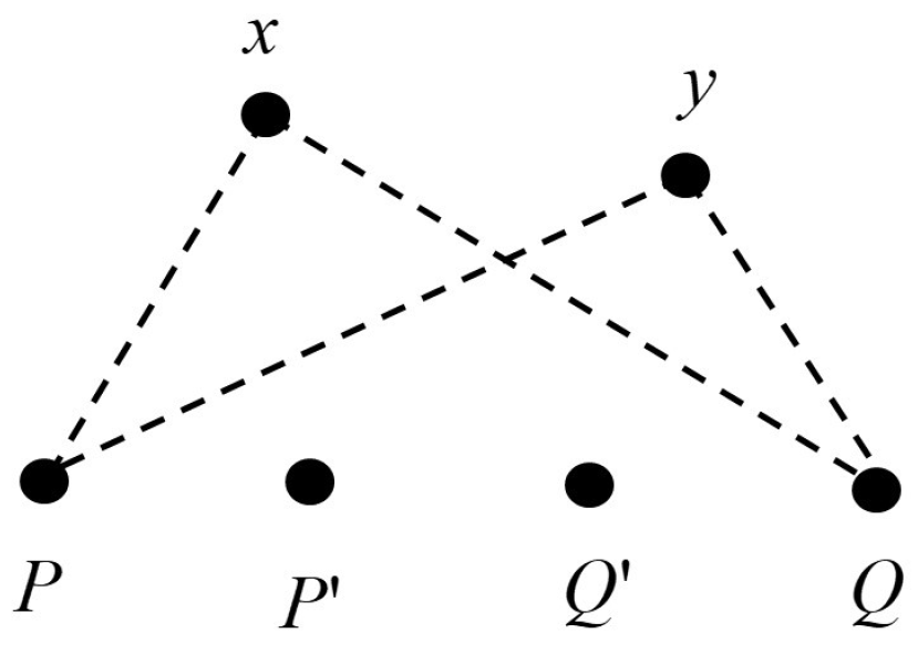
3.1. Collinearity and Subspaces
3.2. Directionality
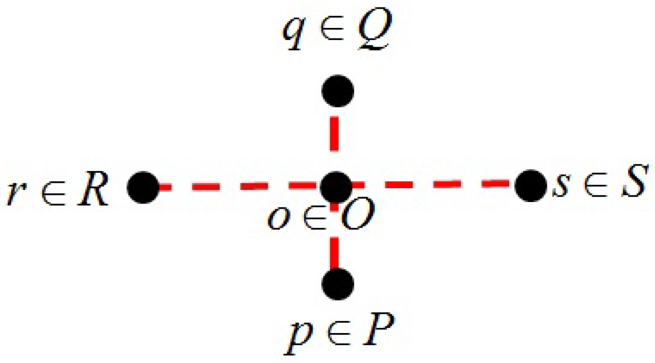
3.3. Coordinated Observers
3.4. Orthogonal Subspaces
3.5. Pythagorean Theorem
4. Simplices
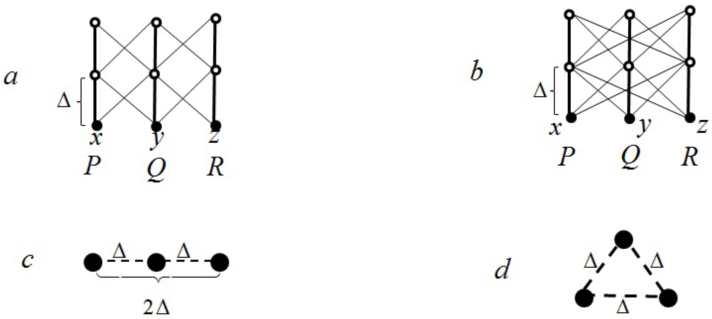
4.1. Discrete Equilateral Triangle
4.2. Discrete Tetrahedron
5. Fence
The Parallel Postulate
6. The Dot Product
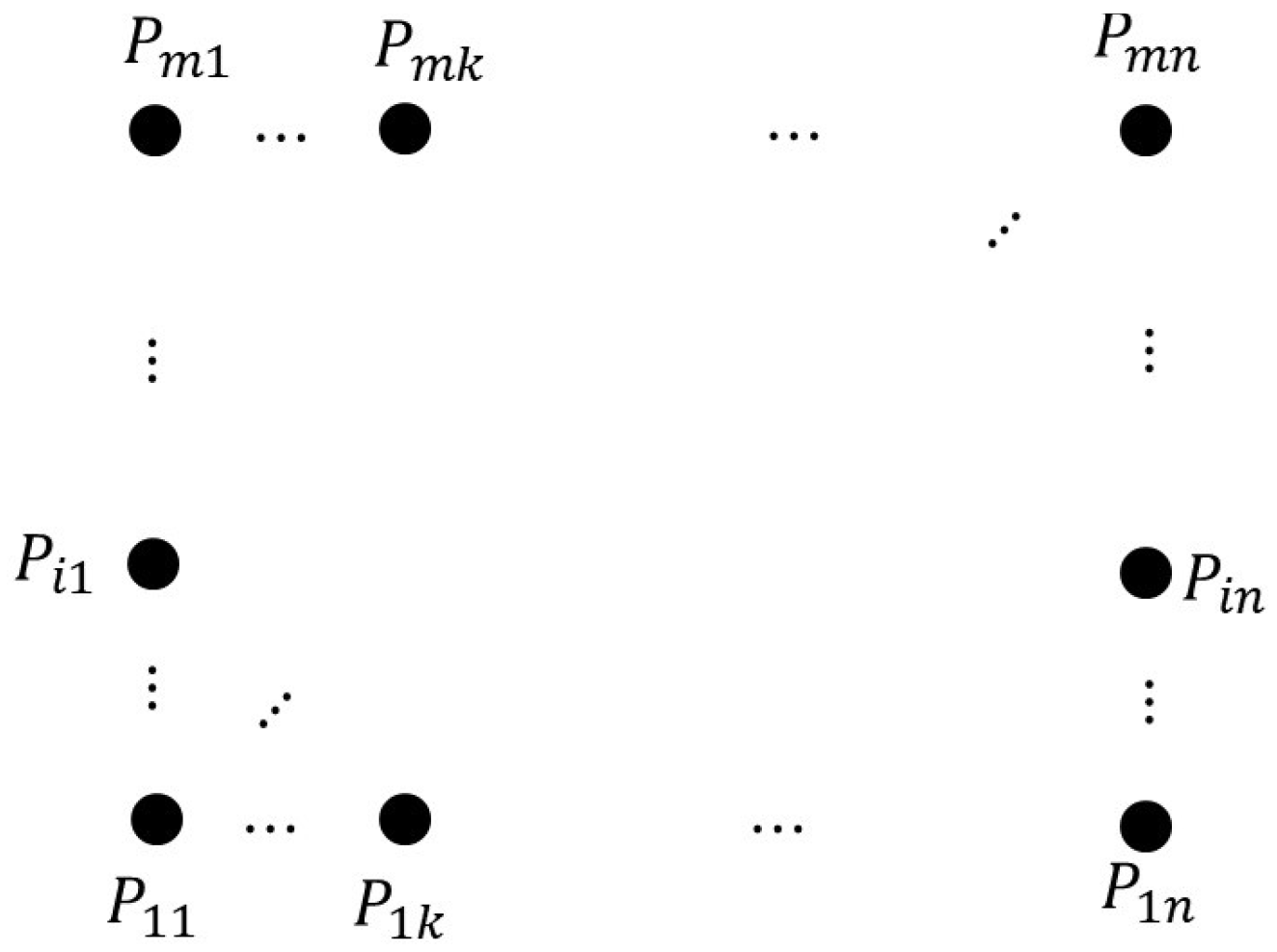
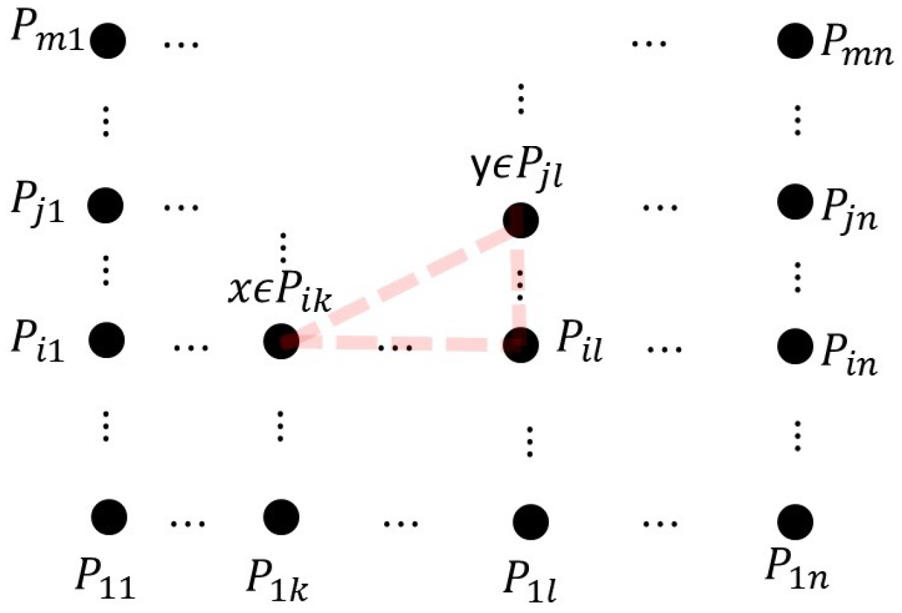
7. Grid
Quantification Inside a Grid
- Special Case I: If and , then .
- Special Case II: If and , then .
- Special Case III: If and , then .
8. Conclusions
- [1]
- We demonstrated that the Pythagorean theorem is derived from the fact that the interval scalars of orthogonal subspaces are additive (see Equation (10)).
- [2]
- [3]
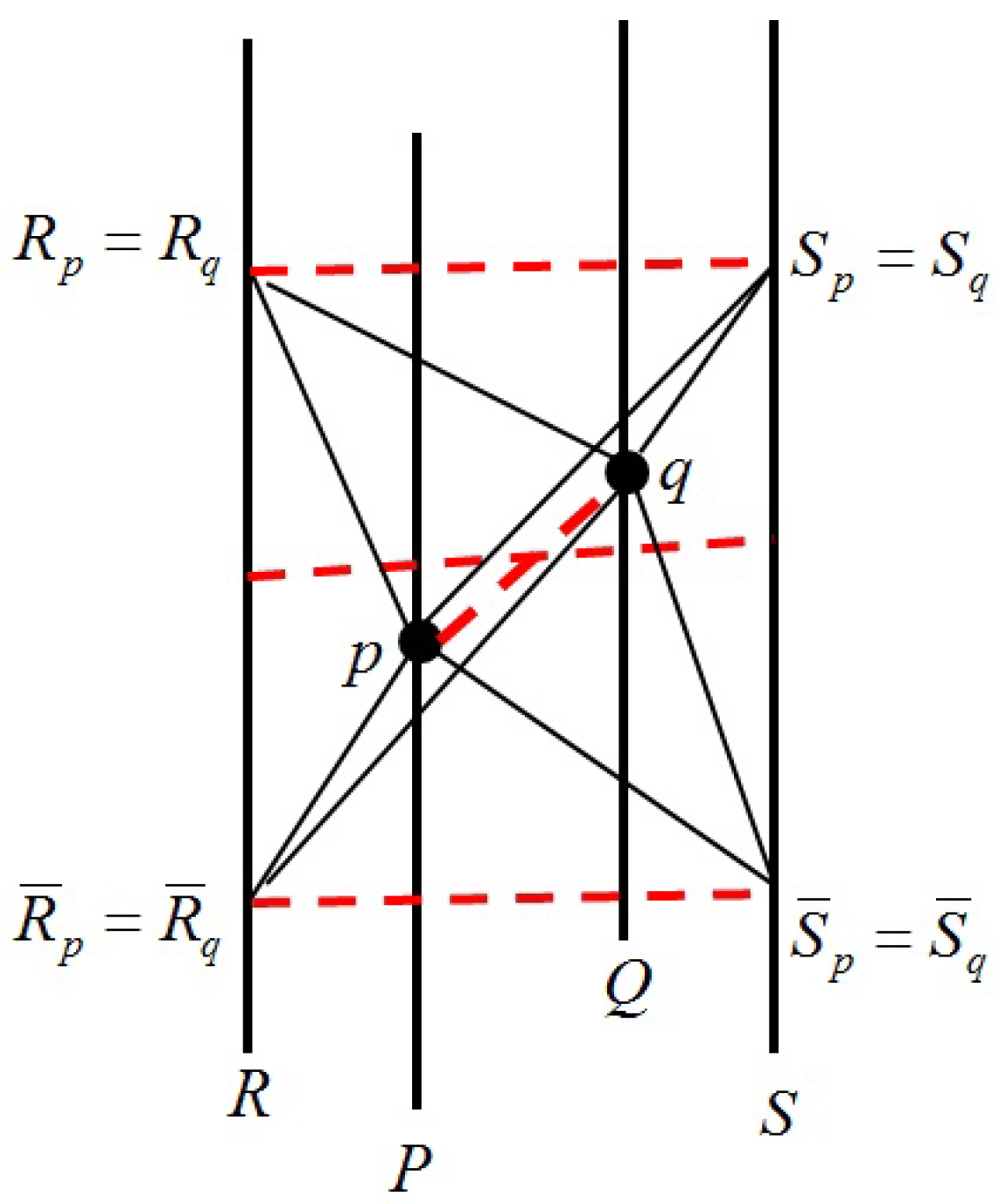
- We introduced the concept of a fence as a set of three or more collinear and coordinated chains. Then, we studied different configurations of two fences. Most importantly, we proved (see Equations (35)–(37)) that fences that share more than one chain and share all chains, which is the equivalent of the parallel postulate in the discrete case.
- [4]
- We found that the projection of an interval onto a set of collinear and coordinated chains results in the dot product (see Equation (54)). The features of the outer (wedge) product in dimensions appeared when quantification was extended from one fence to a number of fences.
- [5]
- Writing the Pythagorean theorem inside a grid, we found a relation whose terms were similar to those of the geometric product squared (see Equation (61)).
Author Contributions
Funding
Data Availability Statement
Acknowledgments
Conflicts of Interest
Appendix A
- Case I:
- Case II:
- Case III:
- Case IV:
- Case V:
- Case I:
- Case II:
- Case III:
- Case IV:
- Case V:
References
- Euclid. The Thirteen Books of The Elements, 2nd ed.; Heath, T., Ed.; Dover: New York, NY, USA, 1956. [Google Scholar]
- Jammer, M. Concepts of Space: The History of Theories of Space in Physics, 2nd ed.; Harvard University Press: Cambridge, MA, USA, 1969. [Google Scholar]
- Einstein, A. On the Electrodynamics of Moving Bodies. Ann. Phys. 1905, 17, 891. [Google Scholar] [CrossRef]
- Knuth, K.H.; Bahreyni, N. A Potential Foundation for Emergent Space-Time. J. Math. Phys. 2014, 55, 112501. [Google Scholar] [CrossRef]
- Knuth, K.H.; Bahreyni, N. The order-theoretic origin of special relativity. In Bayesian Inference and Maximum Entropy Methods in Science and Engineering: Proceedings of the 30th International Workshop on Bayesian Inference and Maximum Entropy Methods in Science and Engineering, Chamonix, France, 4–9 July 2010; Bessiere, P., Bercher, J.-F., Mohammad-Djafari, A., Eds.; American Institute of Physics: Melville, NY, USA, 2011; Volume 1305, pp. 115–121. [Google Scholar]
- Knuth, K.H. Inferences about interactions: Fermions and the Dirac equation. arXiv 2012, arXiv:1212.233. [Google Scholar]
- Knuth, K.H. Information-based physics: An observer-centric foundation. Contemp. Phys. 2013, 55, 12–32. [Google Scholar] [CrossRef]
- Knuth, K.H. Understanding the Electron. arXiv 2015, arXiv:1511.07766. [Google Scholar]
- Knuth, K.H. Information physics: The new frontier. In Bayesian Inference and Maximum Entropy Methods in Science and Engineering: Proceedings of the 30th International Workshop on Bayesian Inference and Maximum Entropy Methods in Science and Engineering, Chamonix, France, 4–9 July 2010; Bessiere, P., Bercher, J.-F., Mohammad-Djafari, A., Eds.; AIP: New York, NY, USA, 2010; Volume 1305, pp. 3–19. [Google Scholar]
- Knuth, K.H. Information-based physics and the influence network. In It from Bit or Bit from It? Springer: Cham, Switzerland, 2013. [Google Scholar]
- Knuth, K.H.; Skilling, J. Foundations of Inference. Axioms 2012, 1, 38–73. [Google Scholar] [CrossRef]
- Sorkin, R.D. Causal Sets: Discrete Gravity, Lectures on Quantum Gravity; Gomberoff, A., Marolf, D., Eds.; Springer: New York, NY, USA, 2005; pp. 305–327. [Google Scholar]
- Sorkin, R.D. Geometry from Order: Causal Sets. Einstein Online 2006, 2, 1007. [Google Scholar]
- Bombelli, L.; Lee, J.-H.; Meyer, D.; Sorkin, R. Spacetime as a Causal Set. Phys. Rev. Lett. 1987, 59, 521–524. [Google Scholar] [CrossRef]
- Bombelli, L.; Meyer, D.A. The origin of Lorentzian geometry. Phys. Lett. A 1989, 141, 226–228. [Google Scholar] [CrossRef]
- Grothus, M.; Vilasini, V. Characterizing signalling: Connections Between Causal Inference and Space-time Geometry. arXiv 2024, arXiv:2403.0091. [Google Scholar]
- Ormrod, N.; Barrett, J. Quantum influences and event relativity. arXiv 2024, arXiv:2401.18005. [Google Scholar]
- Cafaro, C.; Lord, W.M.; Sun, J.; Bollt, E.M. Causation Entropy from Symbolic Representations of Dynamical Systems. Chaos 2015, 25, 043106. [Google Scholar] [CrossRef] [PubMed]
- Cafaro, C.; Ali, S.A.; Giffin, A. Thermodynamic Aspects of Information Transfer in Complex Dynamical Systems. Phys. Rev. 2016, E93, 022114. [Google Scholar] [CrossRef] [PubMed]
- Dukovski, I. Causal structure of Spacetime and Geometric Algebra for Quantum Gravity. Phys. Rev. 2013, D87, 064022. [Google Scholar] [CrossRef]
- Davey, B.A.; Priestley, H.A. Introduction to Lattices and Order; Cambridge University Press: Cambridge, MA, USA, 2002. [Google Scholar]
- Gätzer, G. General Lattice Theory; Birkhäuser: Basel, Switzerland, 2003. [Google Scholar]
- Cafaro, C.; Ali, S.A. The Spacetime Algebra Approach to Massive Classical Electrodynamics with Magnetic Monopoles. Adv. Appl. Clifford Algebr. 2007, 17, 23. [Google Scholar] [CrossRef]
- Doran, C.; Lasenby, A. Geometric Algebra for Physicists; Cambridge University Press: Cambridge, MA, USA, 2003. [Google Scholar]
- Hestenes, D. Spacetime Algebra; Gordon and Breach: New York, NY, USA, 1966. [Google Scholar]
- Cafaro, C. Finite-Range Electromagnetic Interaction and Magnetic Charges: Spacetime Algebra or Algebra of Physical Space? Adv. Appl. Clifford Algebr. 2007, 17, 617. [Google Scholar] [CrossRef]
- Knuth, K.H. Lattice duality: The origin of probability and entropy. Neurocomputing 2005, 67C, 245–274. [Google Scholar] [CrossRef]
- Knuth, K.H. Valuations on lattices and their application to information theory. In Proceedings of the 2006 IEEE International Conference on Fuzzy Systems, Vancouver, BC, Canada, 16–21 July 2006; pp. 217–224. [Google Scholar]
- Knuth, K.H. Measuring on lattices. In Bayesian Inference and Maximum Entropy Methods in Science and Engineering: The 29th International Workshop on Bayesian Inference and Maximum Entropy Methods in Science and Engineering, Oxford, MS, USA, 2009; Goggans, P., Chan, C.-Y., Eds.; AIP: New York, NY, USA, 2009; Volume 1193, pp. 132–144. [Google Scholar]
- Knuth, K.H.; Walsh, J.L. An Introduction to Influence Theory: Kinematics and Dynamics. Ann. Phys. 2019, 531, 1800091. [Google Scholar] [CrossRef]
- Knuth, K.H. Partially Ordered Set. In Enumerative Combinatorics, 2nd ed.; Cambridge University Press: Cambridge, MA, USA, 2011; Volume 1, pp. 241–463. [Google Scholar]
- Birkhoff, G. Lattice Theory, 3rd ed.; American Mathematical Society: Providence, RI, USA, 1967. [Google Scholar]
- Fayyad, U.; Piatetsky-Shapiro, G.; Smyth, P. From Data Mining to Knowledge Discovery in Databases. AI Mag. 1996, 17, 37. [Google Scholar]
- Micciancio, D.; Regev, O. Lattice-Based Cryptography. In Post-Quantum Cryptography; Bernstein, D.J., Buchmann, J., Dahmen, E., Eds.; Springer: Berlin, Germany, 2009; pp. 147–191. [Google Scholar]
- Smyth, M.S.; Martin, J.H. X Ray Crystallography. Mol. Pathol. 2000, 53, 8–14. [Google Scholar] [CrossRef] [PubMed] [PubMed Central]
- Surya, S. Evidence for a Phase Transition in 2D Causal Set Quantum Gravity. Class. Quantum Gravity 2012, 29, 132001. [Google Scholar] [CrossRef]
- Reid, D.D. Manifold dimension of a causal set: Tests in conformally flat spacetimes. Phys. Rev. D 2003, 67, 024034. [Google Scholar] [CrossRef]
- Hawking, S.W.; King, A.R.; McCarthy, P.J. A New Topology for Curved Space-Time which Incorporates the Causal, Differential and Causal Structures. J. Math. Phys. 1976, 17, 174181. [Google Scholar] [CrossRef]
- Malament, D.B. The Class of Continuous Timelike Curves Determines the Topology of Spacetime. J. Math. Phys. 1977, 18, 13991404. [Google Scholar] [CrossRef]
- Surya, S. Causal Set Topology. Theor. Comput. Sci. 2008, 405, 187–197. [Google Scholar] [CrossRef]
- Surya, S. The Causal Set Approach to Quantum Gravity. Living Rev. Relativ. 2019, 22, 5. [Google Scholar] [CrossRef]
- Al-Ghazali, M. The Incoherence of the Philosophers, 2nd ed.; Marmura, M.E., Ed.; Brigham Young University: Provo, UT, USA, 2002. [Google Scholar]
- Futch, M. Leibniz’s Metaphysics of Time and Space; Springer: New York, NY, USA, 2008. [Google Scholar]


Disclaimer/Publisher’s Note: The statements, opinions and data contained in all publications are solely those of the individual author(s) and contributor(s) and not of MDPI and/or the editor(s). MDPI and/or the editor(s) disclaim responsibility for any injury to people or property resulting from any ideas, methods, instructions or products referred to in the content. |
© 2024 by the authors. Licensee MDPI, Basel, Switzerland. This article is an open access article distributed under the terms and conditions of the Creative Commons Attribution (CC BY) license (https://creativecommons.org/licenses/by/4.0/).
Share and Cite
Bahreyni, N.; Cafaro, C.; Rossetti, L. An Observer-Based View of Euclidean Geometry. Mathematics 2024, 12, 3275. https://doi.org/10.3390/math12203275
Bahreyni N, Cafaro C, Rossetti L. An Observer-Based View of Euclidean Geometry. Mathematics. 2024; 12(20):3275. https://doi.org/10.3390/math12203275
Chicago/Turabian StyleBahreyni, Newshaw, Carlo Cafaro, and Leonardo Rossetti. 2024. "An Observer-Based View of Euclidean Geometry" Mathematics 12, no. 20: 3275. https://doi.org/10.3390/math12203275
APA StyleBahreyni, N., Cafaro, C., & Rossetti, L. (2024). An Observer-Based View of Euclidean Geometry. Mathematics, 12(20), 3275. https://doi.org/10.3390/math12203275