Abstract
The concept of probabilistic interval preference ordering sets (PIPOSs) provides a scientific and intuitive framework for solving real-life multi-criteria group decision-making problems. In some areas such as investment decision-making and supplier selection, PIPOSs have a wider application space, and the development of similarity and distance measures based on PIPOSs holds great significance. Similarity measure is a basic and prominent tool for dealing with imperfect and ambiguous information in fuzzy sets, but it can also be used to deal with uncertain information in preference ordering. These metrics play an important role in the actual decision-making process, as they effectively quantify the degree of similarity between two PIPOSs, and further allow for the prioritization of different scenarios. In this article, we sort out the definitions and arithmetic rules of PIPOSs, and creatively propose several new similarity measures based on PIPOSs. Then, we propose a group decision-making method based on similarity measures and conduct a comparative study with three existing similarity measures to illustrate its advantages over existing metrics. Finally, we confirm its validity through numerical illustrations in the case study, and also conduct a comparative assessment to verify the scientific validity and effectiveness of the newly introduced measure against the existing metrics.
Keywords:
interval ordering; probabilistic interval preference ordering; similarity measure; group decision-making MSC:
03B52; 03E72; 94D05
1. Introduction
With the rapid development of digitalization and information technology, the supply chain network has gradually become extensive and complex. In this context, the selection of suppliers or customers is no longer limited by geographic location and the information cocoon, but how to take optimal decision-taking into account regarding the sustainability, resilience, profitability, and other aspects of an enterprise has become a key issue. Many decision-makers try to find a balance under each criterion, but the determination of criterion weights is not an easy task in itself. Decision-makers’ preferences and ranking of alternatives often vary under different proportions of criterion weights. The uncertainty and complexity of supply chains are further enhanced, especially under the influence of the obvious trend of globalization and geopolitical tensions. Such globalized supply chains, while increasing in efficiency and flexibility, also become more fragile and vulnerable to international market fluctuations and policy changes. Therefore, supplier selection should be taken into account not only economic factors, but also diversification and risk diversification in the context of globalization. This requires firms to develop supply chain strategies with a global perspective and adopt more flexible and diversified supplier management strategies to cope with the increasingly complex and uncertain global environment. Therefore, the introduction of preference information models with probabilities and intervals can effectively mitigate this situation.
In practical life, decision-making is often very complex, which may reflect the subjective ambiguity of decision-makers, limitations of knowledge, aversion to alternative solutions, and uncertainty in decision-making problems [1,2]. What is uncertainty? For example, a bank intends to invest in a company and has four companies to choose from: C1, C2, C3, and C4. The bank manager believes that company C1’s business situation and profitability level is more in line with their requirements and can be ranked in the top two, but the top two also hold an uncertain ranking. Because of various factors such as the complexity and variability in the decision-making environment, it is often difficult to make the optimal decision directly, especially in group decision-making, and it can only be limited to a certain preference interval. Multi-criteria group decision-making involves finding the optimal solution among multiple alternatives to solve real-life problems while satisfying multiple criteria. When there is a multi-criteria group decision-making problem, the weights of each criterion will also have a corresponding impact on the results, leading to a more complex decision-making.
In order to solve such a realistic problem, scholars proposed the concept of fuzzy sets to simulate the way the human brain processes information, which was subsequently further developed into interval fuzzy sets, hesitant fuzzy sets, etc., from different perspectives, proposing a variety of similarity and distance measures applicable to fuzzy sets, such as the cosine similarity measure and two-parameter similarity measure [3]. And later, scholars proposed interval preference ranking and its mathematical form, as well as a theoretical model for solving the decision-making problem [4]. In a nutshell, suppose a group decision-making problem has n alternative solutions, m experts, and j criteria. In order to select the best alternative or obtain a ranking of the alternatives, decision-makers need to combine the preference information of the alternatives made based on various criteria into a group selection. This preference information may include ordinal ranking [5,6], language preference relationships [7], intuitive fuzzy preference relationships [8], hesitant fuzzy preference relationships [9], etc. In the above preference information, preference ranking is a convenient and useful decision aid tool that can be used to intuitively represent the decision-makers’ preference information and their evaluation of alternative solutions.
Usually, we think that the decision we make should be a specific ranking, but the decision-maker’s judgment often has uncertainty in reality. Sometimes, the information given by the expert may not be a definite value, but an interval with preference information. The example of bank investment mentioned above is also an expression of such a preference ranking. With the rapid development of society and the emergence of various information technologies, actual decision-making problems become more and more complex, and group decision-making problems become more and more important. At present, there are many group decision-making methods based on preference ranking in the existing literature, as shown in Table 1. The first to propose the candidate ranking problem was Borda and Kendall (known as the Borda–Kendall method). They argued that the final ranking could be determined by the sum of the decision-maker’s rankings of the individual candidates [10]. Based on this, many scholars have begun to study the method of decision-making based on individual preferences to reach group consensus. In concrete terms, some scholars began to use interval numbers, preference rankings or ranking ordinals, and uncertain preference ordinals to represent preference information. Cook and Kress [11,12] developed a model for aggregating ordinal rankings where decision-makers can express the strength of their personal preferences and thus derive a consensus ranking. González-Pachón and Romero [4] proposed an interval goal programming approach to solve the group decision-making problem with incomplete ordinal ranking. Wang and Yang [10] developed a preference aggregation method to rank alternatives by utility interval estimation. Fan [13] constructed a probabilistic decision matrix and a collective probability matrix of alternatives regarding ranking position and obtained the ranking of alternatives by solving the model. Xu [14] proposed a nonlinear programming model that was used to determine the expert relative importance weights and an ideal solution for calculating the positive and negative preference order of the distance collective interval. Xu and Wang [2] proposed a distance-based clustering method to evaluate the relative importance weights and interval preference ranking of GDM. Xu [15] proposed an aggregation-based approach and the TOPSIS approach with probabilistic interval preference orderings for multi-criteria group decision-making.
In addition, some scholars have also used utility values, multiplicative preference relations, fuzzy preference relations, and linguistic variables to represent preference information so as to solve group decision-making problems. For example, Xu and Cai [16] took the interval utility value as a unified preference representation and put forward the group decision consensus process of the interval utility value and interval preference ranking. Wu and Liao [17] proposed a product ranking method that can be used to rank products through consumer-provided preference relationships between them. In recent years, some scholars have also begun to study the use of aggregation operators to solve group decision problems, such as OWA [18], PIPOWA [15], FHFPHM [19], PIOPA [20], and PIOGPA [20].

Table 1.
The literature review.
Table 1.
The literature review.
| Author | Year | Main Content | Measure |
|---|---|---|---|
| Cook, W.D.; Kress, M. [11,12] | 1985 1986 | They proposed a sequential ordering with preference strength and formulated an integer linear programming method to obtain a consistent ordering. | Preference rankings or ranking ordinals |
| Beck, M.P.; Lin, B.W. [21] | 1983 | Beck and Lin [21] developed a program called Maximum Consistency Heuristic to derive consensus rankings that maximize consistency among decision-makers. | Preference rankings or ranking ordinals |
| González-Pachón J.; Romero C. [4] | 2001 | For the group decision-making problem in which the decision-maker cannot give a complete ranking, an interval goal programming (GP) approach is proposed to solve the aggregation case with incomplete ordinal rankings (quasi orders). | Uncertain preference ordinals |
| Herrera, F.; Herrera-Viedma, E.; Chiclana, F. [1] | 2001 | A model was proposed to integrate different preference structures (preference ranking, utility function, and multiplication preference relationship) using multiplication preference relationship as the basis for unified representation. | Multiplicative preference relations |
| Wang, Y.M..;Yang, J.B.; Xu, D.L. [10] | 2005 | Developed a preference aggregation method estimated by utility intervals where preference ranking is associated with utility intervals estimated using a linear programming model and aggregated using a simple additive weighting method. | Utility values |
| Xu, Z.S.; Chen, J. [22,23] | 2008 | Xu and Chen [22,23] developed linear programming models to deal with another type of multi-attribute group decision-making problem, where the attribute weight information is incomplete. The group decision-making problem provided their preferences on alternatives by using interval utility values, the interval fuzzy preference relationship, and interval multiplicative preference relations. | Utility values; fuzzy Preference relations; Multiplicative preference relations |
| Fan, Z.P.; Liu, Y. [24] Fan Z.P.; Yue, Q; Feng, B.; Liu, Y. [13] | 2010 | Fan investigated how to determine the ranking order of alternatives in a group decision-making problem based on the preference information of the number of ordinal intervals and proposed a method to rank the alternatives by building a collective probability matrix about the alternatives in the ranked positions. | Uncertain preference ordinals |
| Xu, Z.S.; Cai, X.Q. [16] | 2013 | Xu and Cai [16] developed a consensus procedure for group decision-making with interval utility values and interval preference orderings. | Utility values |
| Liang, W.; Rodríguez, R.M.; Wang, Y-M.; Goh, M.; Ye, F. [25] | 2023 | Liang et al. [25] proposed an extended Elimination and Choice Translating Reality (ELECTRE) III method based on regret theory in a PIVHFS environment. | Fuzzy preference relations |
| Wu, S.; Zhang, G. [26] | 2024 | Wu and Zhang [26] proposed a new concept pertaining to interval-valued probabilistic uncertain linguistic preference relation and utilized information uncertainty to determine expert weights, and ultimately solved the group decision-making problem. | Multiplicative preference relations |
Distance and similarity measures are two interrelated information measures that can be effectively used to quantify the degree of deviation and similarity between object pairs. The similarity measure is a fundamental and prominent tool for handling imperfect and fuzzy information. They are two important topics in fuzzy set theory that are widely used in decision-making, data mining, medical diagnosis, pattern recognition, and renewable energy management. At present, distance and similarity measures are widely used in fuzzy sets, and many scholars have proposed and optimized many distance and similarity measures [27,28]. However, few scholars have applied these methods to PIPOSs. We think that distance and similarity measures can also be applied to PIPOSs to solve multi-criteria group decision-making problems.
At present, there have been many studies on multi-criteria group decision-making problems, and in this paper, several more similar methods are selected for in-depth comparative analysis; their comparative results are shown in Table 2. Xu [15] proposed a distance measure that can be applied to PIPOSs, and further proposed a multi-criteria group decision-making method based on aggregation operators. After calculating the score function, he chose to compare each alternative with other alternatives to form a possibility degree matrix. Then, he calculated the final score for each alternative solution based on the priority weight formula to obtain the final priority order. Although this group decision-making method based on distance measure integrates the information of intervals, probabilities, and other aspects and combines the distance measure with multi-criteria weights, it is too computationally large, the steps are more complicated, and the applicability is slightly weaker when there are more decision-makers.
Table 2.
Comparative analysis.
Priority degrees based on a hesitation fuzzy set, proposed by Lan et al. [29], used a priority formula for comparing two hesitant fuzzy sets. Although this priority degree method also obtains the priority ranking between various alternative solutions, it ignores factors such as probability and interval, resulting in results that may not be scientifically accurate. Moreover, although it uses a method of dividing by the number of elements to process the length of hesitant fuzzy sets, this method only makes the fuzzy sets have the same length and does not effectively remove biased information. This will also have a certain impact on the results.
Li [30] proposed multiple distance measures suitable for hesitant fuzzy sets, and here, we chose two of them for comparison. In this distance measure based on hesitant fuzzy sets, Li used ideal points to compare various alternative solutions. They are prioritized by comparing the distance between each decision option under different criteria and the ideal point. It not only divides the length of the fuzzy set by the number of elements, but also incorporates hesitation into the formula range. But this method also did not consider probability and the adjustment of parameters, resulting in biased results.
Ruan and Gong et al. [20] proposed the probabilistic interval ordering prioritized averaging (PIOPA) operator and probabilistic interval ordering Gauss–Legendre prioritized averaging operator (PIOGPA). Then, they constructed a new multi-attribute decision-making method based on the PIOGPA operator of probability intervals and used the arithmetic–geometric mean (AGM) algorithm to compute the weights of each attribute in order to solve the multi-criteria group decision-making problem. The method takes into account the priority relationship between multiple attributes and uses the AGM algorithm to optimize the computational steps for more complex decision-making environments, which leads to a complex and computationally intensive procedure for using the method. The increase in the processing of the information may also turn out to have a positive or negative effect on the preference information, leading to results that may deviate from the ideal solution.
In summary, traditional group decision-making problems tend to use hesitant preference relationships, utility values, multiplicative preference relationships, and preference ranking to determine the optimal solution, and the weights and importance of the criteria are often fixed. But in fact, the weight allocation of each criterion has a crucial impact on decision-making, especially when decision-makers face different scenarios, and their decisions are often different. Excessive averaging or setting of weights may result in biased decision outcomes. Therefore, we believe that a method can be introduced to quantify the determination of the weights of each criterion, thereby affecting the ranking of the final decision solution.
However, in existing research, the use of this method to handle real-world group decision-making problems in the PIPOS environment has received little attention from scholars, and the factors considered by various methods, such as intervals, probabilities, preference ranking, and computational complexity, can also have different effects on the optimal solution obtained. In this study, we create a new similarity measure to determine the weight information of each criterion in order to solve the group decision-making problem in PIPOSs and fill the gap in existing research.
We believe that the innovation and value of this study are mainly manifested in the following aspects:
- -
- We combined classic similarity measures with the probabilistic interval preference ordering element (PIPOEs) to create three similarity formulas applicable to PIPOE scenarios. These formulas can be used to measure the degree of similarity and correlation between two PIPOEs.
- -
- Although there are currently some methods that can solve multi-criteria group decision-making problems, most methods are still limited to the number of decision-makers or alternative solutions. When there are too many decision-makers or alternative solutions in a group decision-making problem, existing models and algorithms may find it difficult to calculate the optimal choice. Therefore, we propose a multi-criteria group decision-making method with relatively less computational complexity compared to operator and multiplication preference relationships, mainly reflected in the application of similarity formulas and simplification of steps, while retaining the original scientific information.
- -
- The probability of decision-makers’ preferences varying may also have different impacts on group decision-making. We referred to the method proposed by Xu et al. [15] to characterize interval preference ranking by adding probability parameters, introduced a model for accurately quantifying the weights of each attribute, and considered relevant information such as probability, interval, and decision-maker preferences.
Based on three classical similarity measures of fuzzy sets, we further propose three similarity measures that can be used for PIPOSs. Considering that the application scenarios and variable intervals of a fuzzy set and PIPOS are different, we need to process this formula to make it work in a probabilistic interval ordering environment. Saaty [31] points out that the hierarchical model of a social problem may be from a focus (an overarching goal) down to criteria, down to sub-criteria as subdivisions of criteria, and finally to alternatives for making choices. The two general types of hierarchies are forward and backward process hierarchies, and all of the problems were found to fall into one of these two categories. Therefore, we use analytic hierarchy process to adjust the weights in the formula to make it more scientific and applicable.
In this article, our main research objectives are as follows:
- -
- To develop new similarity measures applicable to PIPOSs and to illustrate the advantages of this method over existing methods through comparison;
- -
- Demonstrate that the similarity measure proposed in this article is scientifically valid through fine proofs and detailed mathematical analysis;
- -
- Developing a new algorithm based on the new PIPOE similarity measure for multi-criteria group decision-making problems;
- -
- Demonstrate numerically the proposed mathematical model.
The structure of this article is as follows: In Section 2, we briefly review the definitions about interval ranking and probabilistic interval preference ordering, as well as their arithmetic rules. In Section 3, we review the existing distance measures for probabilistic interval preference ordering, based on which, we propose three similarity measures applicable to PIPOEs. In Section 4, we develop a model of a group decision-making problem centered on the similarity measure so as to rank alternatives and analyze it in comparison with three other existing group decision-making methods. In Section 5, we apply the model to analyze a real-world problem of supplier selection and design an optimal supplier in a probabilistic interval ranking setting. Finally, we discuss the findings and main points of this paper in the concluding section.
2. Preliminaries
In this section, we first briefly review the basic concepts of interval preference ordering to facilitate the understanding and description of probabilistic interval preference ordering sets. Then, we introduce the concepts of probabilistic interval preference ordering set (PIPOS) and the probabilistic interval preference ordering element (PIPOE) to facilitate the further discussion.
Definition 1
([32]). Let be a set of positive integers. The interval preference orderings can be expressed as
where and . In addition, and are the minimum and maximum values of the ordinal interval preference ordering , respectively. For convenience, the interval ordering can be abbreviated as . Especially when , the interval ordering becomes a definite ordering .
Definition 2
([15]). Let be a fixed set as Definition 1. The probabilistic interval preference ordering set (PIPOS) can be expressed as
where is a set of positive integer intervals, denoting the possible ranking values of the element , and is the probability distribution of . For simplicity of representation, the probabilistic interval preference ordering element (PIPOE) can be expressed as , where and are the lower and upper bounds of the interval and is the corresponding probability. Especially when there are several probabilistic intervals, it can be expressed as , respectively.
Definition 3.
For a PIPOE , the score of can be evaluated by the score function , shown as follows:
where . For convenience, the score function can be expressed as , and can be expressed as .
In order to compare two PIPOEs, Xu [23] gave the possibility degree formula to compare the scores of two PIPOEs; thus, we can obtain the priority of PIPOEs as the following definition show as follows:
Definition 4
([15]). Suppose there are two PIPOEs and the scores of them can be expressed as . The possibility degree formula to compare the scores is given by
Then, we can compare the PIPOEs by using the following rules:
- (1)
- If , then;
- (2)
- If , then;
- (3)
- If , then .
Example 1.
Let and . We can calculate their scores by Definition 3, which is shown as
Then, we can compare the scores by using the possibility degree formula and obtain
Thus, we can obtain the priority that is .
Definition 5
([15]). Let be a PIPOE. The expectation can be expressed as
Definition 6
([15]). Let be a PIPOE. The variance can be expressed as
Then, let be a horizontal section of the normal distribution , where and are the expectation and the standard deviation of the PIPOE , respectively.
Based on the basic operations of addition, subtraction, multiplication, and division in mathematics, we put forward the basic operation rule of PIPOEs. These rules will be helpful for us to carry out the subsequent calculation of similarity measure, as in the following [15]:
Definition 7
([15]). Let and be two PIPOEs. The basic operational rules for PIPOSs can be expressed as
- (1)
- (2)
- (3)
- (4)
- (5)
- (6)
3. Distance and Similarity Measures Between Two PIPOEs
Distance measure, similarity measure, and entropy measure are the most commonly used tools for group decision-making. Most of the existing similarity measures and distance measures are proposed based on the environment of fuzzy sets, which have certain limitations: fuzzy sets only consider factors such as membership and non-membership and ignore the decision-maker’s prioritization among alternatives. Although some fuzzy sets take into account factors such as intuition, hesitation, intervals, and probability, a lot of information is still lost, making the final conclusions biased. To some extent, PIPOSs overcome this limitation. Xu [15] has established the distance measure of probability interval ordering. However, there are fewer studies on similarity metrics for PIPOEs in existing research, and most of the previous researchers focused on similarity measures for fuzzy sets. Based on the similarity measure of fuzzy sets and distance measure of PIPOEs, we further propose the similarity measure of probability interval ordering. In this chapter, we will introduce the following contents: (1) the PIPOS distance measures proposed by Xu [15]; (2) the novel PIPOS similarity measures we propose.
3.1. Drawback of the Existing Distance Measures of PIPOEs
There are three classical distance measures that are most widely used, which are (1) the Hamming distance; (2) the Euclidean distance; (3) the Hausdorff distance.
- (1)
- The Hamming distance [33]:
- (2)
- The Euclidean distance [34]:
- (3)
- The Hausdorff distance [35]:
Xu [15] developed these distance measures to measure the deviations among PIPOEs, respectively, shown as follows:
- (1)
- The probabilistic interval preference ordering normalized Hamming distance:
- (2)
- The probabilistic interval preference ordering normalized Euclidean distance:
- (3)
- The generalized probabilistic interval preference ordering normalized Hausdorff distance:
Then, the deviation of the alternative and the other alternatives with respect to the criterion can be expressed as
3.2. New Similarity Measures between Two PIPOEs
Similarly, according to the similarity measures of fuzzy sets proposed by Hong [36], Liang [37], and Arunodaya [38], we further propose several similarity measures suitable for probability interval ordering. Then, we adjust the formula according to the local weights in the analytic hierarchy process [39], and finally obtain the following three similarity measures (The formula can be found in the Appendix A):
Definition 8.
Let and be two PIPOEs. Then, the similarity measure can be expressed as
where and represent the weight values of the preference ranking corresponding to the interval .
Example 2.
There are two PIPOEs, and , which include 6 alternatives. Then, we obtain
Definition 9.
Let and be two PIPOEs. Then, the similarity measure can be expressed as
When parameter , it is the same as Formula (14); when the parameter , the expression correspondingly becomes as follows:
where and represent the weight values of the preference ranking corresponding to the interval .
Example 3.
There are two PIPOEs, and , which include 6 alternatives. Then, we obtain
Definition 10.
Let and be two PIPOEs. Then, the similarity measure can be expressed as
Example 4.
There are two PIPOEs, and . Then,
Definition 11.
For a PIPOE , the final score of can be evaluated by the score function shown as follows:
where and represents the number of alternatives.
4. Multi-Criteria Group Decision-Making with PIPOEs
In a multi-criteria group decision problem, we assume that there are alternatives , criteria , and decision-makers . Then, PIPOS can be obtained by summarizing the scores made by each decision-maker according to the criteria. The PIPOE represents the interval preference ordering of alternative according to criterion . For convenience, we use the PIPOE to represent it. In the following chapters, we summarize the methods proposed by Xu [15] to remove inaccurate information and determine criterion weights, and then we first propose the multi-criterion group decision method based on probability interval order similarity measure.
4.1. Adjustment of Inaccurate Information in PIPOEs
In actual decision-making, the special preference of the decision-makers may have some effect on the interval preference ordering, such as too high or too low. This may lead to bias in group decision-making. In mathematics, scholars believe that the distribution of such values approximates the normal distribution [15]. Thus, we apply the normal distribution to remove the “biased” information and redistribute the probability of interval preference ordering.
In order to adjust the “biased” information and reassign the probabilities of interval preference orderings, we use the Algorithm 1 proposed by Xu [15] to deal with the PIPOEs.
| Algorithm 1. Algorithm for Normalizing Preference Information. |
| Step1. Judge the relationship between each element of PIPOE and according to Definition 3 and Formula (4). |
|
Since all of the information of PIPOE is in the form of interval preference ordering, the smaller the interval value, the better the PIPOE. Therefore, if or , then should be deleted; otherwise, it should be retained. Step2. After removing the “biased” information, we obtain the adjusted PIPOE , where the probability can be calculated by the formula , and . Step3. Compare each element of the adjusted PIPOE and again according to Formula (4). Therefore, if or , then should be deleted; otherwise, it should be retained. Step4. Until all the adjusted elements are retained, go to Step 5. Otherwise, go back to Step 2 and repeat the procedure. Step5. End. |
4.2. Similarity Method for Multi-Criterion Group Decision
In the multi-criterion group decision-making problem, the weight value of each criterion is different because of their differing importance. For an alternative, the more similar it is to the optimal decision, the better it should be rated. In reality, however, there is rarely a single alternative that meets the preferences of all decision-makers. If an alternative has the greatest similarity to the optimal decision under all criteria, then it is most likely the best option in reality. In the following, we develop a multi-criterion group decision-making method based on the similarity measure:
Step1. Decision-makers provide their preferences according to different criteria and alternatives, which are collated and aggregated in a PIPOS .
Step2. The PIPOEs contained in the PIPOS are compared with , and biased information is further deleted according to possibility degree Formula (4). Then, we use Algorithm 1 to obtain the adjusted PIPOS , and is the adjusted PIPOE.
Step3. Calculate the similarity values using Formula (16) under each criterion, and form the similarity matrix S (the same as Formulas (14) and (15)).
Step4. Add the similarity of different decisions corresponding to each criterion, and calculate the weight corresponding to each criterion by the Lagrange multiplier method:
Then, we can obtain the weight of the criterion:
Step5. Calculate the score of the adjusted PIPOE , and calculate the matrix P by the possibility degree formula.
Step6. Use the weight calculation formula to obtain the final scores:
Then, we obtain the final ranking according to the scores.
In order to facilitate a better understanding of the method proposed in this study, we try to use Figure 1 to describe the whole process and its steps, shown as follows:
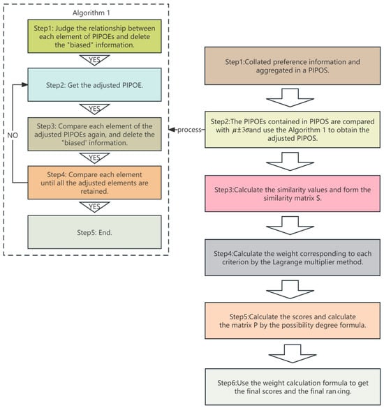
Figure 1.
Flow chart of the similarity measure of PIPOEs.
5. Application of the Proposed PIPOS Similarity Measures in Supply Chain Management
In recent years, with the rapid development of the digital economy, the deep integration of a new generation of information technology and logistics technology has given birth to the development model of smart logistics. Smart logistics characterized by digitization, intelligence, networking, green, visualization, and flexibility have incorporated automated execution, intelligent operation, and intelligent decision-making in all aspects of logistics operation [40]. At present, China is and may be facing the situation of weak growth of foreign trade and domestic demand for a long time, and the diversified digital supply chain structure can better meet the new needs of diversification and differentiation in the market, which is also more in line with the realistic requirements of supply chain modernization development. In April 2018, the Chinese State Council announced the “Notice on Carrying out Supply Chain Innovation and Application Pilot”, which, as a landmark event in the construction of smart supply chain, aims to use smart hardware, the Internet of things, big data, and other digital technology means to accelerate supply chain logistics, capital flow, and information flow integration. The promotion of the supply chain intelligence upgrade, which is typical of integration, intelligence, automation, and interconnection, will inevitably have a potential impact on supply chain resilience and enterprise performance. In addition, the emergence of the COVID-19 disruption has caused a wide range of breaks in the global supply chain, and scholars have further realized the importance of combining supply chain resilience and digital technology [41,42]. A common definition of supply chain resilience is the ability of a supply chain to quickly recover to a normal state in the face of a devastating major shock [43], which is closely related to supply chain disruptions. To build supply chain resilience, we first need to consider and assess the source and degree of supply chain risk, that is, the main source and impact of the challenge to supply chain resilience. Part of the supply chain disruption risk comes from the uncertainty of the external environment, and the other part comes from the competitiveness of the supply chain itself. The existence of these realistic factors makes enterprises have to consider the sustainability and efficiency of the supply chain when selecting suppliers, such as the comparative analysis of supplier flexibility, agility, collaboration, visibility, and digitization degree [44,45].
Flexibility includes process flexibility, response flexibility, time-based flexible management, and strategic flexibility [46]. Realistic factors include the uncertainty of market demand and the frequency of product changes, which make enterprises need to have supply chain flexibility. Choosing a flexible supplier ensures the flexibility to adjust production capacity, lead times, etc., to meet market demand as it changes. Adaptation, anticipation, recovery, absorption, dispersion, delay, and reactivity are part of agility [47]. Market competition is fierce, and enterprises need to respond quickly to changes, including the launch of new products, changes in market trends, etc. Choosing an agile supplier ensures that production, supply, etc. can be quickly adjusted to maintain a competitive advantage when the market changes. Collaboration includes not only the sharing of resources, knowledge, strategies, and information about risks, but also integration among social organizations, as well as relationship quality, collaborative forecasting, risk and benefit sharing, information sharing, technical capabilities among partners, and collaboration and coordination among stakeholders [48]. All aspects of the supply chain need to work closely together, including raw material supply, processing and manufacturing, and logistics and distribution. Choosing a supplier with good collaboration ensures efficient coordination between all parts of the supply chain, thereby improving overall operational efficiency. Supply chain visibility includes a set of actions that highlight predictive analytic, market visibility, supplier visibility, technology visibility, and scenario building [49]. Practical factors include the information flow in the supply chain is not smooth, information is not transparent, etc. These factors make enterprises need to choose suppliers with good visibility to ensure the full control of the supply chain links. Through real-time monitoring and transparent information exchange, enterprises can timely understand the problems in the supply chain and take appropriate measures to solve them to ensure the sustainability of the supply chain. Digitization includes data collection and storage, data analysis and mining, collaboration and collaboration tools, automation and intelligence, as well as visualization and monitoring, enabling information sharing, decision support, and business optimization by transforming information and processes in the supply chain into digital form. Practical factors include the rapid development of information technology and the momentum of digital transformation, which make enterprises need to choose suppliers with a high degree of digitization. Digital capabilities can provide more accurate data analysis, more efficient information exchange, more accurate production planning, and more, thereby improving the efficiency and sustainability of the supply chain.
In this case, in order to evaluate the suppliers and select the best solution, the decision-maker needs to evaluate the suppliers’ flexibility, agility, collaboration, visibility, and digitization. There are four suppliers as alternatives, namely, C1, C2, C3, C4, C5, and C6. There are dozens of decision-makers who provide information about their preferences. For convenience, we provide PIPOEs here to represent its evaluation values and probability distribution, as shown in Figure 2.
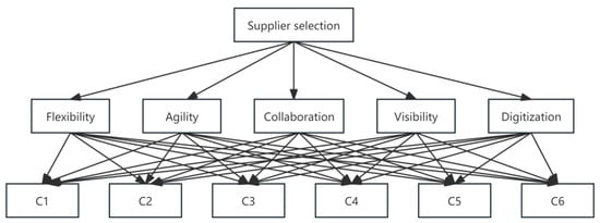
Figure 2.
Metrics and alternatives of supplier selection.
Based on these indicators, the values are shown in Table 3 [15].
Table 3.
The evaluation values.
5.1. The Similarity Measure of PIPOS
Step1. According to the decision-maker’s preference information for each alternative under each criterion, we collect and organize PIPOEs as shown in Table 3.
Step2. We use Algorithm 1 to deal with the original PIPOE and remove the “biased information” in the preference information. By comparing the PIPOS with and deleting “biased information”, we obtain the adjusted PIPOS as Table 4:
Table 4.
The adjusted evaluation values.
Step3. We calculate the similarity values of alternatives based on the criteria by Formula (16), as shown in Table 5:
Table 5.
The similarity values.
After that, we add the similarity values of the corresponding alternatives under each criterion and obtain the following:
Step4. We calculate the weight vector corresponding to each criterion by Formula (18) and obtain the weight vector, which is derived as
Step5. Now, we use Formula (3) to calculate the scores of the adjusted PIPOEs, which are shown in Table 6:
Table 6.
The scores of the adjusted PIPOEs.
Then, we can obtain the final scores by Equation (17), and the results are shown in Figure 3.
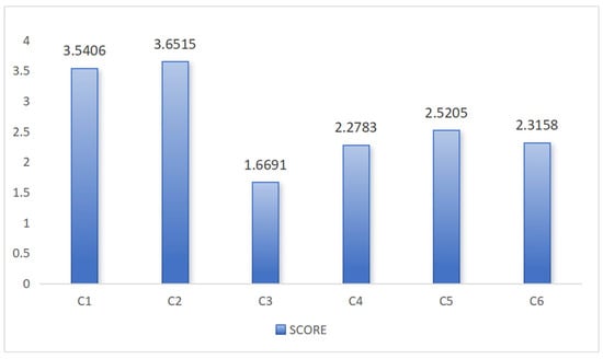
Figure 3.
The score for each supplier in the case analysis.
Finally, the suppliers are ranked as follows according to the scores:
5.2. Sensitivity Analysis
The above results were obtained under the assumption of Formula (16). Then, we used Formula (15) with parameters for sensitivity analysis to further validate the scientific validity of the model. In order to observe the changes in the optimal solution under different parameter values, without loss of generality, we assigned different parameters of 0.25, 0.5, 1, 2, 4, 10, and 20. The specific sorting results calculated using the similarity measure are shown in Table 7.
Table 7.
Sensitivity analysis of different parameter values (Formula (15)).
Figure 4 clearly illustrates the score values and their trends for each alternative solution when the parameter values change.
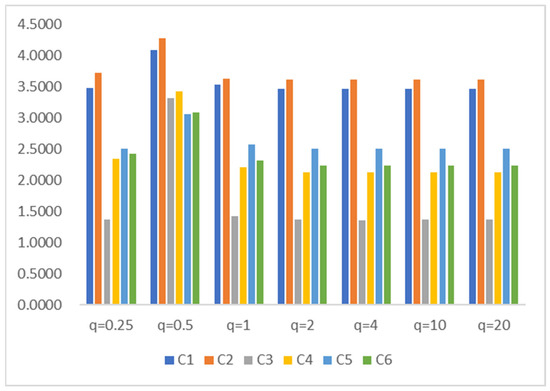
Figure 4.
The score for each alternative when is different.
Figure 5 and Figure 6 further clarify the sensitivity of the score values of each scheme to the variation in parameter values when is different.
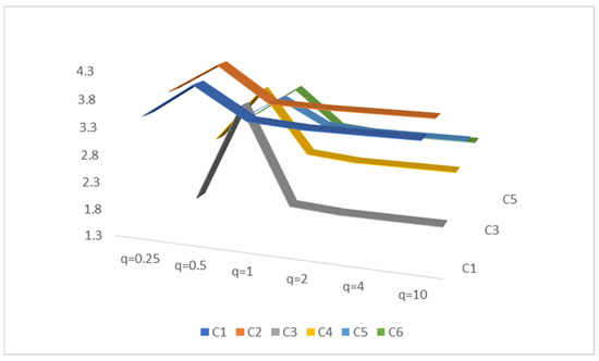
Figure 5.
The parameter sensitivity of the score values for each alternative when is different.
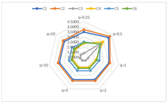
Figure 6.
The final scores of each alternative.
According to the results shown in Table 7 and Figure 5, it can be observed that when the parameter values change, the score of the scheme slightly changes, but the ranking remains basically unchanged. Specifically, when the allocated parameter is greater than or equal to 1, the sorting result remains unchanged. However, when the parameter is less than 1, significant changes in ranking (the ranking is when ) may be due to the use of similarity formulas to calculate negative values, and the addition of values from each criterion cancels out the positive and negative values, affecting the accuracy of the results. Therefore, we tested again whether taking the absolute value of the formula as a whole can yield similar results as before when the parameter is equal to 0.5. The data results show that the ranking is still . In this study, we did not further confirm the scientific validity of taking absolute values, which requires further analysis and discussion in subsequent research.
In addition, the sorting results remain consistent with the increase in parameter values, demonstrating the stability and reliability of the PIPOS-based similarity measure. Further analysis shows that the scores of each alternative solution fluctuate on a small scale with the increase in parameters, which may be the result of decision-makers’ risk preference changes in different contexts. Although the overall ranking may change, the optimal solution remains unchanged. This indicates that the parameter has no significant impact on the selection of the optimal solution. Therefore, decision-makers can choose appropriate parameters based on personal preferences when evaluating.
5.3. Comparison
In order to further compare and analyze the scientific validity and effectiveness of the decision-making methods proposed in this article, four different methods are selected in this section for comparative analysis with the methods proposed in this paper. The results of the comparative analysis are summarized and shown in Table 8 and Figure 7.
Table 8.
Comparative analysis of different measures.
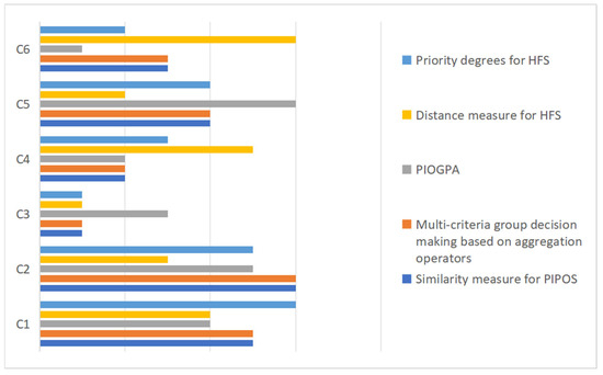
Figure 7.
Comparative analysis of different measures.
In the comparative analysis, both the similarity measure proposed in this paper and the distance measure proposed by Xu [15] use the algorithm of probabilistic interval preference ordering, and both of them take into account the problem of weighting different attributes as well as the use of normal distribution for the raw preference information collected. The difference is that the former adopts the way of setting ideal points to evaluate the scores of each alternative from the perspective of measuring the similarity between the alternatives and the ideal points so as to obtain the final optimal solution. The latter, on the other hand, uses a distance measure to assess the attribute weights, and the prioritization between the alternatives is obtained by applying the aggregation operator to calculate the weights of each alternative. From the results, the ordering of the programs obtained by both methods is consistent: . Side by side, this also proves the scientific validity and effectiveness of the methodology proposed in this paper. Moreover, the steps of this measure are relatively simple and more widely applicable. Moreover, PIOGPA, proposed by Ruan et al. [20], and the method proposed in this paper consider probability and preference ranking, as well as the weighting problem between different attributes. The difference is that the former proposes a new aggregation operator and calculates the preference ranking of alternatives from the perspective of the AGM algorithm. However, due to the different focuses considered by the two schemes, the final results obtained may also present some deviations.
Assuming that the decision-makers have the same probability of preference for the values in each interval, it is possible to approximate the transformation of this probabilistic interval-ordered group decision problem into a multi-attribute group decision problem with hesitant fuzzy sets. If the product of the boundary values of the intervals and the probabilities of the intervals is taken as the corresponding hesitant fuzzy values, then the corresponding PIPOE can be transformed into an HFE. Therefore, the preference information we mentioned in the case study can also be transformed into information in the HFS environment. Based on this, we compare and analyze the method proposed in this paper with the priority degrees for HFSs proposed by Lan and Jin [29]. The method proposed by Lan and Jin [29] for the multi-attribute decision-making problem with known attribute weight information and uncertain fuzzy attribute values is to obtain a new conversion decision matrix by multiplying each attribute weight value with the HFE. Since different number of HFEs may appear in the application, they adopted the rule proposed by Xu and Wang [50] to process the elements into elements of the same length, and further calculated the converted decision matrix according to the limited formula for hesitant fuzzy set to obtain the final result. However, this approach ignores the importance of the weights between the attributes and does not take into account the preference ordering between the schemes, focusing only on the problem of affiliation. This will cause a lot of detail information to be lost in the process, which will further lead to bias in the final results. By calculating the priority of each alternative by this measure, we obtained the ranking of alternatives as follows:
This simply demonstrates the priority level of one alternative relative to another, but this priority level does not represent an absolute ranking relationship in reality. As a result, we can see that the final results presented deviate slightly from the results we obtained.
The main characteristic of distance measurement based on the HFS is to only consider the differences between element values, without considering the differences in weight and number of elements between different attributes. The HFS focuses on the hesitancy in providing membership values, manifested as differences between values and differences in the number of elements. Therefore, ignoring the impact of unit quantity differences may lead to unreasonable results. When calculating the ideal alternative for the HFS, Li [30] used the same ideal value as in this article, which is . We selected the best alternative by calculating the distance between each alternative and the ideal alternative. We present the results in Table 9 and Table 10. However, as with the previous methods, the neglect of the importance of attribute weights and interval ordering led to a degree of bias in the final results. Although the authors attempted to increase the number of parameters and the degree of affiliation in the algorithm to further refine the results, the lack of preference information led to even more severe bias.
Table 9.
Results obtained by distance measure .
Table 10.
Results obtained by distance measure .
By summarizing the comparative analysis results of the above four methods, we believe that the similarity measure model proposed in this paper has a wider application range. Specific instructions are as follows:
- (1)
- The proposed measure formula considers both preference interval and probability. By introducing intervals and probabilities, the preference information of decision-makers can be quantified more accurately. By using probability, decision-makers can better express the uncertainty and variability inherent in attribute weights, making decision models more realistic and flexible.
- (2)
- The proposed group decision method combines a similarity measure with an ideal point and is used to quantify the importance of each attribute. At the same time, by assigning different values to parameters, more choices are provided for decision-makers. Decision-makers can choose different parameters according to personal preferences when making decisions, so it is more flexible and practical.
- (3)
- Compared with other methods, the method proposed in this paper has the advantage of measuring the similarity between each alternative point and the ideal point in relatively simple and computationally fewer steps, also using this as the basis for calculating the priority of each alternative. The computational work mainly focuses on Algorithm 1 and Formula (18). However, when there are large numbers of alternatives and decision-makers, they may also face a relatively large number of calculations.
- (4)
- Despite the above advantages, there are still limitations. This limitation is mainly manifested in that when the parameter is less than 1, there may be a large sorting difference in the use of this method, which may be due to the characteristics of exponential functions. The method should be further improved in order to improve its scientificity and effectiveness.
6. Conclusions
The PIPOE is a convenient tool for expressing and evaluating decision-makers’ preferences. However, in the existing literature, the importance of the possible evaluation value is usually ignored, and few scholars have proposed distance measures and similarity measures based on interval preference ordering. First of all, we comb the concept of PIPOSs, which includes all preference information and its importance degrees provided by decision-makers, as well as its basic component, the PIPOE. In this study, we continue to follow the operation rules and properties of PIPOEs proposed by Xu [15], which provides us with basic operation tools for the subsequent calculation of group decision problems with probability interval preference ordering. Then, we propose three similarity measures based on probability interval preference ordering specificity and apply them to our proposed multi-criterion group decision-making method. Due to the uniqueness of PIPOEs, when there is a large number of decision-makers and their preferences are different, PIPOEs can express the preference information of decision-makers in an intuitive and convenient way. So, we propose a multi-criterion group decision-making method based on PIPOEs and their similarity measure. Considering that decision-makers may give too high or too low interval preference ordering, we use Algorithm 1 [15] that uses a normal distribution to remove inaccurate information in the PIPOE and redistribute the probability interval preference ordering, and then we obtain the adjusted PIPOE. In order to obtain the optimal alternative, we assume that there is an optimal interval ordering . We use similarity measure Formulas (14)–(16) to calculate the similarity between interval preference of each alternative and the optimal preference ordering . The higher the similarity values between the alternative and optimal interval ordering , the better the score it obtains. Based on this, we calculate the weight of each criterion and the final scores of the alternatives and obtain the priority ranking of the alternatives. The group decision-making method is then justified through a case study and compared with four other existing group decision-making methods to demonstrate its effectiveness and applicability.
We believe that the novelty and importance of this approach lies in the fact that we have created a similarity measure that is applicable to the PIPOE environment and have proposed a model that can be used to solve the group decision-making problem by determining the weighting attributes of each criterion. In this model, we pay attention to the importance of the weights of the criteria, the interval of preference information, and the probability, which will be introduced into the computational steps. In addition, we try to explore a method to directly compare the similarity with the ideal decision and obtain the final solution ranking from the ideal point, which means that the optimal solution we obtain will be the closest to the ideal decision. Case results demonstrate that this approach is feasible.
Although we attempted to organize and propose similarity metrics applicable to the PIPOE environment from the perspective of the existing literature and achieved relatively good results, there are some limitations to the approach proposed in this paper: First, the similarity formula proposed in this study is directly applied to the weights of the relevant criteria for measuring preference information, which means that they have a relatively weak impact on the ranking results. The intervals and probabilities to which the preference information belongs may have a greater impact on the ranking results. This is the reason why in the sensitivity analysis, the change in the scores of the alternatives is weaker when the parameter is greater than 2. Second, when the parameter is chosen to be less than 1, the results of the formula may be negative. This phenomenon is more obvious, as the parameter tends to be closer to 0. This may originate from the characteristics of the exponential function, which lead to a change in the ranking results. Subsequently, this requires more in-depth research and optimization of the formula to improve its usability and scientificity. Finally, although we try to make simplifications to the formula and take steps to reduce the amount of computation, we may still face the problem of computational difficulties when there are more alternatives and decision-makers. In addition, this paper is based on the similarity metric in the HFS environment and further proposes a similarity metric with hierarchical analysis. Therefore, subsequent scholars may try to develop other similarity metrics or adjust the parameters to improve their scientific validity, on the basis of which they may propose a more scientific group decision-making method to reduce the excessive interference of other factors.
Author Contributions
Q.W., R.W. and C.-Y.R. conceived the algorithm; Q.W., R.W. and C.-Y.R. validated the methodology; Q.W. and R.W. wrote the original manuscript; Q.W., R.W. and C.-Y.R. analyzed the results; Q.W. and C.-Y.R. supervised the writing process; Q.W. provided the funding. All authors have read and agreed to the published version of the manuscript.
Funding
This research was funded by the National Natural Science Foundation of China (NSFC) Youth Program: “The Impact of Differentiated Relationship Strength in Core Supplier Networks on Supplier Participation in Firms’ Innovation Performance” (72102050).
Data Availability Statement
Data is contained within the article.
Conflicts of Interest
The authors declare no conflicts of interest.
Appendix A
In order to facilitate readers in better understanding some proper nouns in this article, we provide the abbreviation table for readers to quickly query, shown as Table A1.
Table A1.
Abbreviations.
Table A1.
Abbreviations.
| Abbreviation | Full Name and Main Formula |
|---|---|
| PIPOE | probabilistic interval preference ordering element |
| PIPOS | probabilistic interval preference ordering set |
| Formula (14) | |
| Formula (15) | |
| Formula (16) | |
| Formula (17) | |
| Formula (18) | |
| Formula (19) |
References
- Herrera, F.; Herrera-Viedma, E.; Chiclana, F. Multiperson decision-making based on multiplicative preference relations. Eur. J. Oper. Res. 2001, 129, 372–385. [Google Scholar] [CrossRef]
- Xu, Y.; Wang, H.; Sun, H.; Yu, D. A distance-based aggregation approach for group decision making with interval preference orderings. Comput. Ind. Eng. 2014, 72, 178–186. [Google Scholar] [CrossRef]
- Hanan, A.; Abdul, R.; Humaira, A.; Dilshad, A.; Umer, S.; Jia-Bao, L. Improving Similarity Measures for Modeling Real-World Issues with Interval-Valued Intuitionistic Fuzzy Sets. IEEE Access 2024, 12, 10482–10496. [Google Scholar]
- Gonzalez-Pachon, J.; Romero, C. Aggregation of partial ordinal rankings: An interval goal programming approach. Comput. Oper. Res. 2001, 28, 827–834. [Google Scholar] [CrossRef]
- Cook, W.D.; Kress, M.; Seiford, L.M. A general framework for distance-based consensus in ordinal ranking models. Eur. J. Oper. Res. 1996, 96, 392–397. [Google Scholar] [CrossRef]
- Cook, W.D. Distance-based and ad hoc consensus models in ordinal preference ranking. Eur. J. Oper. Res. 2006, 172, 369–385. [Google Scholar] [CrossRef]
- Herrera, F.; Herrera-Viedma, E. Linguistic decision analysis: Steps for solving decision problems under linguistic information. Fuzzy Sets Syst. 2000, 115, 67–82. [Google Scholar] [CrossRef]
- Xu, Z.S. Intuitionistic preference relations and their application in group decision making. Inf. Sci. 2007, 177, 2363–2379. [Google Scholar] [CrossRef]
- Liao, H.C.; Xu, Z.S. A VIKOR-based method for hesitant fuzzy multi-criteria decision making. Fuzzy Optim. Decis. Mak. 2013, 12, 373–392. [Google Scholar] [CrossRef]
- Wang, Y.M.; Yang, J.B.; Xu, D.L. A preference aggregation method through the estimation of utility intervals. Comput. Oper. Res. 2005, 32, 2027–2049. [Google Scholar] [CrossRef]
- Cook, W.D.; Kress, M. Ordinal ranking with intensity of preference. Manag. Sci. 1985, 31, 26–32. [Google Scholar] [CrossRef]
- Cook, W.D.; Kress, M. Ordinal ranking and preference strength. Math. Soc. Sci. 1986, 11, 295–306. [Google Scholar] [CrossRef]
- Fan, Z.P.; Yue, Q.; Feng, B.; Liu, Y. An approach to group decision-making with uncertain preference ordinals. Comput. Ind. Eng. 2010, 58, 51–57. [Google Scholar] [CrossRef]
- Xu, Z. Group decision making model and approach based on interval preference orderings. Comput. Ind. Eng. 2013, 64, 797–803. [Google Scholar] [CrossRef]
- He, Y.; Xu, Z.; Jiang, W. Probabilistic Interval Reference Ordering Sets in Multi-Criteria Group Decision Making. Int. J. Uncertain. Fuzziness Knowl.-Based Syst. 2017, 25, 189–212. [Google Scholar] [CrossRef]
- Xu, Z.; Cai, X. On Consensus of Group Decision Making with Interval Utility Values and Interval Preference Orderings. Group Decis. Negot. 2013, 22, 997–1019. [Google Scholar] [CrossRef]
- Wu, X.; Liao, H. Managing uncertain preferences of consumers in product ranking by probabilistic linguistic preference relations. Knowl.-Based Syst. 2023, 262, 110240. [Google Scholar] [CrossRef]
- Nguyen, J.; Armisen, A.; Sánchez-Hernández, G.; Casabayó, M.; Agell, N. An OWA-based hierarchical clustering approach to understanding users’ lifestyles. Knowl.-Based Syst. 2020, 190, 105308. [Google Scholar] [CrossRef]
- Ruan, C.Y.; Chen, X.J.; Han, L.N. Fermatean Hesitant Fuzzy Prioritized Heronian Mean Operator and Its Application in Multi-Attribute Decision Making. Comput. Mater. Contin. 2023, 75, 3204–3222. [Google Scholar] [CrossRef]
- Ruan, C.Y.; Gong, S.C.; Chen, X.J. Probabilistic Interval Ordering Prioritized Averaging Operator and Its Application in Bank Investment Decision Making. Axioms 2023, 12, 1007. [Google Scholar] [CrossRef]
- Beck, M.P.; Lin, B.W. Some heuristics for the consensus ranking problem. Comput. Oper. Res. 1983, 10, 1–7. [Google Scholar] [CrossRef]
- Xu, Z.S.; Chen, J. MAGDM linear programming models with distinct uncertain preference structures. IEEE Trans. Syst. Man Cybern. Part B 2008, 38, 1356–1370. [Google Scholar] [CrossRef]
- Xu, Z.S.; Chen, J. Some models for deriving the priority weights from interval fuzzy preference relations. Eur. J. Oper. Res. 2008, 184, 266–280. [Google Scholar] [CrossRef]
- Fan, Z.P.; Liu, Y. An approach to solve group-decision-making problems with ordinal interval numbers. IEEE Trans. Syst. Man Cybern. 2010, 40, 1413–1423. [Google Scholar]
- Liang, W.; Rodríguez, R.M.; Wang, Y.-M.; Goh, M.; Ye, F. The extended ELECTRE III group decision making method based on regret theory under probabilistic interval-valued hesitant fuzzy environments. Expert Syst. Appl. 2023, 231, 120618. [Google Scholar] [CrossRef]
- Wu, S.; Zhang, G. Incomplete interval-valued probabilistic uncertain linguistic preference relation in group decision making. Expert Syst. Appl. 2024, 243, 122691. [Google Scholar] [CrossRef]
- Chen, S.M. Measures of similarity between vague sets. Fuzzy Sets Syst. 1995, 74, 217–223. [Google Scholar] [CrossRef]
- Kumar, R.; Kumar, S. A novel intuitionistic fuzzy similarity measure with applications in decision-making, pattern recognition, and clustering problems. Granul. Comput. 2023, 8, 1027–1050. [Google Scholar] [CrossRef]
- Lan, J.; Jin, R.; Zheng, Z.; Hu, M. Priority degrees for hesitant fuzzy sets: Application to multiple attribute decision making. Oper. Res. Perspect. 2017, 4, 67–73. [Google Scholar] [CrossRef]
- Li, D.; Zeng, W.; Zhao, Y. Note on distance measure of hesitant fuzzy sets. Inf. Sci. 2015, 321, 103–115. [Google Scholar] [CrossRef]
- Saaty, R.W. The analytic hierarchy process—What it is and how it is used. Math. Model. 1987, 9, 161–176. [Google Scholar] [CrossRef]
- Sun, M.; Liang, Y.Y.; Pang, T.J. A weighted ranking method of dominance rough sets for interval ordered information systems. Comput. Syst. 2018, 39, 676–680. [Google Scholar]
- Bustince, H.; Burillo, P. Correlation of interval-valued intuitionistic fuzzy sets. Fuzzy Sets Syst. 1995, 74, 237–244. [Google Scholar] [CrossRef]
- Mesquita, D.P.P.; Gomes, J.P.P.; Souza Junior, A.H.; Nobre, J.S. Euclidean distance estimation in incomplete datasets. Neuro Comput. 2017, 248, 11–18. [Google Scholar] [CrossRef]
- Hung, W.L.; Yang, M.S. Similarity measures of intuitionistic fuzzy sets based on Hausdorff distance. Pattern Recognit. Lett. 2004, 25, 1603–1611. [Google Scholar] [CrossRef]
- Hong, D.H.; Kim, C. A note on similarity measures between vague sets and between elements. Inf. Sci. 1999, 115, 83–96. [Google Scholar] [CrossRef]
- Liang, Z.; Shi, P. Similarity measures on intuitionistic fuzzy sets. Pattern Recogn. Lett. 2003, 24, 2687–2693. [Google Scholar] [CrossRef]
- Arunodaya, R.M.; Dragan, P.; Hezam, I.M.; Chakrabortty, R.K.; Rani, P.; Božanić, D.; Ćirović, G. Interval-Valued Pythagorean Fuzzy Similarity Measure-Based Complex Proportional Assessment Method for Waste-to-Energy Technology Selection. Processes 2022, 10, 1015. [Google Scholar] [CrossRef]
- Tavana, M.; Soltanifar, M.; Santos-Arteaga, F.J. Analytical hierarchy process: Revolution and evolution. Ann. Oper. Res. 2023, 326, 879–907. [Google Scholar] [CrossRef]
- Fosso, W.S.; Gunasekaran, A.; Dubey, R.; Ngai, E.W.T. Big data analytics in operations and supply chain management. Ann. Oper. Res. 2018, 270, 1–4. [Google Scholar] [CrossRef]
- Alvarenga, M.Z.; Oliveira, M.P.V.; Oliveira, T.A.G.F. The impact of using digital technologies on supply chain resilience and robustness: The role of memory under the COVID-19 outbreak. Supply Chain. Manag. Int. J. 2023, 28, 825–842. [Google Scholar] [CrossRef]
- Liu, H.; Lu, F.; Shi, B.; Hu, Y.; Li, M. Big data and supply chain resilience: Role of decision-making technology. Manag. Decis. 2023, 61, 2792–2808. [Google Scholar] [CrossRef]
- Hussain, G.; Nazir, M.S.; Rashid, M.A.; Sattar, M.A. From supply chain resilience to supply chain disruption orientation: The moderating role of supply chain complexity. J. Enterp. Inf. Manag. 2023, 36, 70–90. [Google Scholar] [CrossRef]
- Roque Júnior, L.C.; Frederico, G.F.; Costa, M.L.N. Maturity and resilience in supply chains: A systematic review of the literature. Int. J. Ind. Eng. Oper. Manag. 2023, 5, 1–25. [Google Scholar] [CrossRef]
- Huang, Y.-F.; Phan, V.-D.-V.; Do, M.-H. The Impacts of Supply Chain Capabilities, Visibility, Resilience on Supply Chain Performance and Firm Performance. Adm. Sci. 2023, 13, 225. [Google Scholar] [CrossRef]
- Thomas, A.; Byard, P.; Francis, M.; Fisher, R.; White, G.R.T. Profiling the resiliency and sustainability of UK manufacturing companies. J. Manuf. Technol. Manag. 2016, 27, 82–99. [Google Scholar] [CrossRef]
- Dabhilkar, M.; Birkie, S.E.; Kaulio, M. Supply-side resilience as practice bundles: A critical incident study. Int. J. Oper. Prod. Manag. 2016, 36, 948–970. [Google Scholar] [CrossRef]
- Namdar, J.; Li, X.; Sawhney, R.; Pradhan, N. Supply chain resilience for single and multiple sourcing in the presence of disruption risks. Int. J. Prod. Res. 2018, 56, 2339–2360. [Google Scholar] [CrossRef]
- Naz, F.; Kumar, A.; Majumdar, A.; Agrawal, R. Is artificial intelligence an enabler of supply chain resiliency post COVID-19? An exploratory state-of-the-art review for future research. Oper. Manag. Res. 2022, 15, 378–398. [Google Scholar] [CrossRef]
- Wang, H.; Xu, Z. Admissible orders of typical hesitant fuzzy elements and their application in ordered information fusion in multi-criteria decision making. Inf. Fusion 2016, 29, 98–104. [Google Scholar] [CrossRef]
Disclaimer/Publisher’s Note: The statements, opinions and data contained in all publications are solely those of the individual author(s) and contributor(s) and not of MDPI and/or the editor(s). MDPI and/or the editor(s) disclaim responsibility for any injury to people or property resulting from any ideas, methods, instructions or products referred to in the content. |
© 2024 by the authors. Licensee MDPI, Basel, Switzerland. This article is an open access article distributed under the terms and conditions of the Creative Commons Attribution (CC BY) license (https://creativecommons.org/licenses/by/4.0/).