Fast and Compact Partial Differential Equation (PDE)-Based Dynamic Reconstruction of Extended Position-Based Dynamics (XPBD) Deformation Simulation

Abstract

Dynamic simulation is widely applied in the real-time and realistic physical simulation field. How to achieve natural dynamic simulation results in real-time with small data sizes is an important and long-standing topic. In this paper, we propose a dynamic reconstruction and interpolation method grounded in physical principles for simulating dynamic deformations. This method replaces the deformation forces of the widely used eXtended Position-Based Dynamics (XPBD), which are traditionally derived from the gradient of the energy potential defined by the constraint function, with the elastic beam bending forces to more accurately represent the underlying deformation physics. By doing so, it establishes a mathematical model based on dynamic partial differential equations (PDE) for reconstruction, which are the differential equations involving both the parametric variable u and the time variable t. This model also considers the inertia forces caused by acceleration. The analytical solution to this model is then integrated with the XPBD framework, built upon Newton’s equations of motion. This integration reduces the number of design variables and data sizes, enhances simulation efficiency, achieves good reconstruction accuracy, and makes deformation simulation more capable. The experiment carried out in this paper demonstrates that deformed shapes at about half of the keyframes simulated by XPBD can be reconstructed by the proposed PDE-based dynamic reconstruction algorithm quickly and accurately with a compact and analytical representation, which outperforms static B-spline-based representation and interpolation, greatly shortens the XPBD simulation time, and represents deformed shapes with much smaller data sizes while maintaining good accuracy. Furthermore, the proposed PDE-based dynamic reconstruction algorithm can generate continuous deformation shapes, which cannot be generated by XPBD, to raise the capacity of deformation simulation.

1. Introduction

In recent years, there has been a noticeable increase in the demand for high-quality simulations across various domains, driven by advancements in technology and computational capabilities. This surge is evident in fields ranging from engineering and physics to medicine and virtual environments. The quest for more immersive and realistic simulations has led to the integration of cutting-edge technologies like augmented reality and digital twins. However, the quality and fidelity of visual results remain critical factors influencing the effectiveness of simulations. As such, researchers and developers are constantly exploring novel approaches to enhance the realism and accuracy of simulations, leveraging mathematical models and computational techniques to achieve more lifelike results. This paper aims to contribute to this endeavor by presenting a novel method focused on the mathematical and computational aspects of simulation.

Physics-based simulations mimic how objects move and change based on real-world physics principles, aiming for precise results. However, these simulations need a lot of computing power and time, which can make them impractical for real-time applications. On the other hand, data-driven simulations can achieve realistic results by training on many example models with detailed deformations. But, this approach often requires a lot of human effort, which may not be feasible for designers. Neither method fully meets the demands of the real-time gaming industry, as detailed models with realistic animations require more design parameters like polygons and vertices, which can be challenging to handle.

Position-based deformation methods provide an effective solution for achieving natural movement in real-time environments without putting too much strain on computational resources. These techniques offer a fresh approach to simulating deformation, enabling researchers and game developers to produce stable and reliable results in a computationally efficient way. By focusing directly on the position layer and skipping traditional physical parameters like velocity and acceleration, these methods offer a high level of control. Additionally, by integrating shape-matching and data-driven techniques, they enhance their versatility. The speed of simulation and the visually plausible outcomes of position-based methods have made them increasingly favored in the game industry.

Position-based methods have made strides in enhancing deformation simulation, but they have not fully tackled the challenges related to game models. Game models need to be small in size and efficient for real-time rendering since they are typically generated to interact with players. To achieve this, mesh simplification techniques [1,2] have been developed. These methods either reduce the number of design parameters from high-resolution models or create low poly models from scratch. However, low-resolution 3D models may not deliver the natural and precise animations needed for advanced games. To balance computational efficiency and model detail, various techniques like motion prediction and anti-aliasing have been introduced. Among these, the level of detail (LOD) is crucial in modern open-world games like Elden Ring and Grand Theft Auto V. It significantly saves computational resources by reducing model details when they are out of the player’s view. While LOD has eased the burden of more realistic models, the reconstruction of the simplified mesh remains a challenge that needs addressing.

Static ODE-based sweeping surfaces provide a mathematical representation of complex models, maintaining realistic details while reducing data size for easier user control. As shown in Figure 1, the face model on the left contains 8221 vertices and 15,378 polygons, while the ODE-based reconstructed model on the right contains only 4764 vertices and 4236 polygons, reducing by $42.05\%$ and $72.45\%$ respectively. Despite this significant reduction, the reconstructed model retains the most visual details, illustrating the method’s effectiveness in reducing design variables while preserving important features.

Although static ODE-based methods have been utilized for modeling 3D shapes, they cannot consider the dynamic effects of movements and deformations. To address this limitation and make static ODE-based methods useful for creating realistic animations, we introduce the underlying physics of deformation into Newton’s equation of motion to develop a PDE-based dynamic reconstruction method and combine it with extended position-based dynamics to achieve a compact and quick reconstruction of simulation results with good accuracy and a stronger ability to generate new deformed shapes for more natural and efficient deformations in animations. Here, we use the term compact to describe a few design variables and small storage amount.

The work described in this paper makes the following contributions:

• Developing a PDE-based dynamic reconstruction method to recreate deformation models from a series of keyframes with high efficiency, good accuracy, and small data sizes;
• Integrating the PDE-based dynamic reconstruction method with XPBD simulation to reduce keyframes simulated by XPBD and raise the simulation efficiency of deformable objects;
• Constructing a powerful surface representation from elementary functions in closed form solutions to dynamic PDEs to raise the capacity in complicated PDE-based dynamic reconstruction.

2. Related Work

When creating computer-animated characters, it is important to achieve the realistic deformation of detailed models, as it greatly impacts the overall realism of the animation. Shape deformation and geometric model creation can be combined to achieve this aim. In this section, we briefly review shape deformation and geometric model creation techniques.

2.1. Shape Deformation Approaches

Shape deformation involves manipulating a set of control vertices to deform the models. There are four main categories of techniques used for deformation: geometric, physics-based, data-driven, and position-based methods. Each of these techniques offers its own advantages and disadvantages and can be chosen based on the specific requirements of the animation project.

2.1.1. Geometric Approaches

Geometric methods include geometric skinning, Free-Form Deformation (FFD), cage-based deformations, and differential coordinates. Here, we briefly review geometric skinning and FFD.

Linear Blend Skinning (LBS) was the first provided method of geometric skinning, and has been used as a baseline standard in real-time applications for a long time due to its simplicity [3]. However, the quality of the deformation is often poor, with some artifacts, such as the notorious collapsing elbows.

Many other methods such as [4,5,6,7] have been provided to improve the notorious drawback of LBS, including the candy wrapper effect, rigid transformations, and topology dependency, though they all have their own bulging artifacts. For example, based on Delta Mush deformer (DM) [8], Le and Lewis introduced Direct Delta Mush skinning (DDM) [9], which reduces iterations and synchronization of Delta Mush deformer to perform at run-time. This deformer introduces a corrective layer, named “mushing” by the authors, to the skinning process, which effectively mitigates the candy wrapper effect by allowing for more controlled vertex movements. As DM is produced to reduce the authoring cost by avoiding weight-painting, it can handle complex joint movements. Therefore, DDM can create more non-rigid transformations, like realistic skin sliding and muscle bulging. The deformer does not require up-front tweaking and adapts the changes to the rig or model. Due to its independence with model topology, the applications of DDM in rigging allow for more effectiveness and versatility in character design. By addressing the common artifacts of LBS, DDM enables more natural and flexible character deformations, which enhances the overall visual fidelity and realism in animation quality.

Free-Form Deformation (FFD) was introduced to deform solid models in a free-form manner using a structural hyperpatch [10]. Coquillart introduced Extended Free-Form Deformation (EFFD) [11], which uses non-parallelepipedical 3D lattices, defined by users. This method offers more sophisticated control of lattices and supports higher-dimensional lattices. Thus, it can generate complex shapes more accurately and intuitively compared with FFD. Relying on EFFD, Animated Free-Form Deformation (AFFD) [12] was proposed, which is interactive, intuitive, and can be integrated into most traditional animation systems. AFFD introduces the capability to animate deformations over time, allowing objects to morph in a user-controlled manner, which enables the achievement of complex animation. The integration with animation workflows makes it popular in the film and game industry. Discontinuous Free-Form Deformation (DFFD) [13] is an algorithm for modeling cuts and openings in general meshes, which is followed by a manipulation of the control volume of the deformation function. DFFD allows for the application of deformations in a segmented discontinuous manner and enables localized changes to specific regions of the object without affecting the entire mesh. It can effectively manage complex geometries where traditional continuous deformations might struggle. These advancements in FFD reflect ongoing efforts to improve control, realism, and efficiency in the deformation process.

Purely geometric deformation methods are known to be efficient, simple, and low cost. However, they cannot create realistic shape deformation due to lacking in the underlying physics.

2.1.2. Physcis-Based Approaches

In contrast to geometric methods, physics-based deformation techniques use physical laws to compute the deformation, resulting in more natural movement and deformation, particularly in materials that exhibit complex behaviors. Thus, these techniques can handle dynamic interactions between objects and environments more effectively, like colliding responses between objects, stress, and strain. The interactive behaviors lead to the simulation of deformation over time, taking into account factors including fatigue or wear. These factors significantly enhance the realism of long-term simulations. Physics-based deformation techniques can incorporate other principles like energy conservation. The incorporation allows for more realistic animations where energy is transferred during deformations, like in the case of bouncy materials. While purely geometric methods can be simpler and faster for certain applications, particularly in controlled environments, physics-based deformation techniques provide a richer and more immersive experience, especially in interactive simulations and animations that require a high level of realism.

The most simple and easy-to-implement method among all physics-based techniques is the mass-spring system method [14]. However, mass-spring systems often rely on linear spring dynamics, which can oversimplify the behavior of real materials, leading to unrealistic responses to forces and interactions. This oversimplifying problem would further cause penetration or unrealistic bounce effects due to the challenging management in collisions and interactions with other objects. For highly elastic or stiff materials, this system requires very small time steps for stability, making simulations computationally expensive and less efficient. Moreover, mass-spring systems may not accurately conserve energy, particularly in dynamic simulations, leading to unnatural motion or damping effects. Thus, this method struggles to accurately represent complex behaviors, such as plastic deformation or non-linear responses.

The particle-based system method [15] can represent a wider variety of materials by simulating each particle’s individual properties and interactions, allowing for more complex behaviors like plasticity and fluid dynamics. This method can incorporate non-linear forces and adaptive resolution, enabling more natural simulations of deformable bodies. The penetration issues and interaction artifacts between objects can be reduced by integrating collision detection and response mechanisms. In addition, particle-based systems can maintain energy conservation more effectively by modeling forces at the particle level. In contrast to the mass-spring system method, this method can provide greater flexibility and realism as well as significantly reduce computational costs.

Other methods, such as the finite element method (FEM) [16], finite difference method (FDM) [17], boundary element method (BEM) [18], and finite volume method (FVM) [19] have also been developed. Among them, FEM has been widely applied in scientific calculations and engineering analyses due to its capability of dealing with complicated situations and performance in achieving high computational accuracy. Since physics-based approaches achieve impressive realistic results, they have been applied in various fields, such as simulating wear effects in the punching process [20] and ring rolling deformation [21].

2.1.3. Data-Driven Approaches

Data-driven deformation approaches are a class of techniques that leverage machine learning to capture information from the real world and produce detailed simulation results [22,23,24]. Rather than relying on mathematical models, these methods use example deformations as samples to interpolate in-between poses and drive the deformation. The key advantage of data-driven approaches is their ability to capture the complexity of real-world deformation with a relatively small amount of data. However, they require a significant amount of preprocessing to generate the training data and can be computationally expensive during the training phase.

2.1.4. Position-Based Approaches

To further achieve realistic deformation results in real-time applications, Müller et al. first presented a method called position-based dynamics (PBD) [25]. Compared to other methods, PBD has relatively low computational costs and provides visually plausible simulation results. Its speed, robustness, high controllability, and simplicity have made it a popular choice in the game industry. However, PBD also has its limitations like convergence problems, dependence problems between stiffness and time step, and handling order problems of constraints. Methods like the hierarchical position-based dynamics (HPBD) [26] and the multi-grid-based strategy [27] were proposed to improve the solver’s efficiency in reaching convergence. The dependence problem that constraints could be arbitrarily stiff due to the iteration number and time step size has also been well researched, and various developments have been introduced. Among these methods, projective dynamics (PD) [28] and extended position-based dynamics (XPBD) [29] stand out as being particularly popular. They not only enhance the performance of position-based dynamics (PBD) but have also been extended for various other applications. XPBD modifies the PBD solver to obtain a stiff and consistent solution without regarding time step size, while PD introduces additional constraints to the solver in order to reduce reliance on the stiffness and iteration count. In this paper, we will utilize XPBD as the simulation foundation for our simulations, as it offers more precise predictions of constraints for force-dependent effects compared to PBD.

2.2. Geometric Model Creation Approaches

Efforts have been made to increase the computational efficiency of shape deformation methods by using a suitable geometric model creation method. These methods can be categorized into two types based on whether they involve underlying physics: geometric and physics-based methods.

2.2.1. Geometric Approaches

Mainstream geometric model creation methods include polygon modeling, patch modeling, and subdivision modeling. While polygon modeling provides detailed models, it fails to represent curved surfaces accurately [30]. Patch modeling like Bézier modeling [31,32,33] and NURBS modeling [34] could create smooth curved models while relying on heavy human involvement in stitching patches together [35]. Subdivision modeling subdivides faces of coarse polygonal models into smaller ones by interpolation or approximation, leading to denser and more detailed models, but precise subdivision precision is difficult to achieve due to underlying parametrization [36]. Despite these advancements, these geometric modeling methods still have limitations in achieving sufficient realism and easy manipulation. The latter was addressed in various research works to reconstruct some local areas without affecting the whole surface, like that of Bouhiri et al. using a local spline quasi-interpolant method [37].

2.2.2. Physics-Based Approaches

Physics-based modeling approaches can generate more realistic surface shapes by considering the underlying physics. You et al. proposed an ODE-based sweeping surface method, which uses a vector-valued ODE to sweep a curve along two boundary curves while adhering to continuity constraints [38]. Unlike traditional polynomial-based methods such as Bézier, B-Spline, and NURBS, this method uses more complex mathematical functions, which are computationally efficient and numerically stable, even with small data sizes. Various developments of this method have been made, like ODE-based surface blending [39] and ODE-based skin deformations [40]. Similar to ODE-based methods, PDE-based methods were developed to represent free-form surfaces [41]. They were then integrated with interactive design [42], static [43] and dynamic [44] 3D reconstruction, skin deformation [45], and real-time surface manipulation [46].

This paper presents an enhanced approach for dynamic PDE-based modeling to improve dynamic 3D reconstruction capacity and integrates it with extended position-based dynamics (XPBD) to quickly produce detailed deformation results with a continuous and compact representation. Using this method allows for representing deformed shapes with much fewer design variables and smaller data storage, replacing numerous keyframe models typically simulated using extended position-based dynamics with more efficient dynamic PDE-based reconstruction to achieve a considerable reduction in the computational time needed for the simulation process, and creating new deformed shapes at different frames by varying the time variable t within the range of $0\le t\le 1$ to raise the capacity of the deformation simulation.

3. Basis of Position-Based Dynamics

Position-based dynamics (PBD) stands as a widely acclaimed and adaptable simulation framework extensively employed in computer graphics and animation to replicate intricate physical phenomena. In contrast to traditional methodologies relying on explicit equations of motion, PBD adopts a distinctive approach by making positions the central variables for simulation. The objective of this section is to offer a simple and clear explanation of the fundamental principles that form the foundation of position-based dynamics as well as its improvements in XPBD.

3.1. Algorithm Overview

The simulation of the basic PBD could be roughly separated into three steps [47]:

• Prediction: estimating the velocity and position of each vertex at the next time step.
• Correction: applying constraints to rectify the position in solvers.
• Updating: using the corrected position to recompute the relative attributes, including velocities and accelerations.

3.2. The Improvements in XPBD

Position-based dynamics has limitations related to convergence and dependency issues. Various improvements have been made to tackle these issues. Among them, XPBD [29] is highlighted due to its ability to address the problem of iteration count and time step-dependent constraint stiffness.

XPBD introduces Newton’s equations of motion subject to forces $\mathbf{F}\left(\mathbf{x}\right)$:

$$\mathbf{M}\ddot{\mathbf{x}}=\mathbf{F}\left(\mathbf{x}\right)=-\nabla U^T\left(\mathbf{x}\right),$$

(1)

where $\mathbf{x}={[x_1,x_2,\dots ,x_n]}^T$ and $\mathbf{M}=[m_1,m_2,\dots ,m_n]$, $x_i(i=1,2,\dots ,n)$ and $m_i(i=1,2,\dots ,n)$ are the position and mass at the $i^{th}$ point. $\ddot{\mathbf{x}}$ represents the second derivative of $\mathbf{x}$ with respect to time t, and $\mathbf{F}\left(\mathbf{x}\right)$ are forces. $U^T\left(\mathbf{x}\right)$ stands for the energy potential, which is defined as

$$U\left(\mathbf{x}\right)=0.5\mathbf{C}{\left(\mathbf{x}\right)}^T{\gamma }^{-1}\mathbf{C}\left(\mathbf{x}\right),$$

(2)

where $\mathbf{C}\left(\mathbf{x}\right)={[C_1\left(\mathbf{x}\right),C_2\left(\mathbf{x}\right),\dots ,C_m\left(\mathbf{x}\right)]}^T$ is a vector consisting of m constraint functions, and $\gamma$ is a block diagonal compliance matrix derived from stiffness.

Introducing the central finite difference, the acceleration $\ddot{x}$ at time step n can be determined by

$$\ddot{\mathbf{x}}={\displaystyle \frac{{\mathbf{x}}^{n+1}-2{\mathbf{x}}^n+{\mathbf{x}}^{n-1}}{\Delta t^2}},$$

(3)

where $\Delta t$ is a time increment.

Substituting Equation (3) into Equation (1) and using ${\mathbf{x}}^n$ to replace $\mathbf{x}$ in $\mathbf{F}\left(\mathbf{x}\right)$, we obtain the following equation of calculating ${\mathbf{x}}^{n+1}$

$${\mathbf{x}}^{n+1}={\mathbf{x}}^n+\Delta t{\mathbf{v}}^n+\Delta t^2{\mathbf{M}}^{-1}\mathbf{F}\left({\mathbf{x}}^n\right).$$

(4)

A Lagrange multiplier $\mathit{\lambda }$ is introduced and connected to the block diagonal compliance matrix $\gamma$ through the following equation:

$$\mathit{\lambda }=-{\tilde{\gamma }}^{-1}\mathbf{C}\left(\mathbf{x}\right),$$

(5)

where $\tilde{\gamma }={\displaystyle \frac{\gamma }{\Delta t^2}}$.

If the position $\mathbf{x}$ and the Lagrange multiplier $\mathit{\lambda }$ at the $i^{th}$ iteration are known, i.e., $x_i$ and ${\mathit{\lambda }}_i$ are known, the increment $\Delta \mathbf{x}$ and the increment $\Delta \mathit{\lambda }$ can be determined by the following equations:

$$[\nabla \mathbf{C}\left({\mathbf{x}}_i\right){\mathbf{M}}^{-1}\nabla \mathbf{C}{\left({\mathbf{x}}_i\right)}^T+\tilde{\gamma }]\Delta \mathit{\lambda }=-\mathbf{C}\left({\mathbf{x}}_i\right)-\tilde{\gamma }{\mathit{\lambda }}_i,$$

(6)

$$\Delta \mathbf{x}={\mathbf{M}}^{-1}\nabla \mathbf{C}{\left({\mathbf{x}}_i\right)}^T\Delta \mathit{\lambda }.$$

(7)

Having known the velocities ${\mathbf{v}}^n$ and positions ${\mathbf{x}}^n$ at the $n^{th}$ step, the pseudocode of using the XPBD algorithm to calculate the velocities ${\mathbf{v}}^{n+1}$ and positions ${\mathbf{x}}^{n+1}$ at the ${(n+1)}^{th}$ step is summarized in Algorithm 1, where the total number J of solver iterations is specified by the users, and $\Delta \mathit{\lambda }$ and $\Delta \mathbf{x}$ are determined by Equations (6) and (7), respectively.

Algorithm 1 XPBD algorithm

1: initialize ${\mathit{\lambda }}_0=0,{\mathbf{x}}_0={\mathbf{x}}^n+\Delta t{\mathbf{v}}^n+\Delta t^2{\mathbf{M}}^{-1}\mathbf{F}\left({\mathbf{x}}^n\right)$   2: for j∈$[0,J-1]$ do   3:     for all constraints do   4:       calculate ${\mathit{\lambda }}_{j+1}={\mathit{\lambda }}_j+\Delta \mathit{\lambda }$   5:       calculate ${\mathbf{x}}_{j+1}={\mathbf{x}}_j+\Delta \mathbf{x}$   6:     end for   7: end for   8: ${\mathbf{x}}^{n+1}={\mathbf{x}}_J$   9: ${\mathbf{v}}^{n+1}={\displaystyle \frac{{\mathbf{x}}^{n+1}-{\mathbf{x}}^n}{\Delta t}}$

In Algorithm 1, line 1 initializes the state variables, Line 4 uses Equation (6) to determine $\Delta \mathit{\lambda }$ and calculate ${\mathit{\lambda }}_{j+1}={\mathit{\lambda }}_j+\Delta \mathit{\lambda }$, Line 7 uses Equation (7) to determine $\Delta \mathbf{x}$ and calculate ${\mathbf{x}}_{j+1}={\mathbf{x}}_j+\Delta \mathbf{x}$, Line 8 updates the positions, and Line 9 updates the velocity.

3.3. XPBD Simulation

In this paper, we use XPBD to simulate the shape deformation of selected 3D models for over 200 frames on an Intel i7 9700 CPU with a clock rate of 4.7 GHz for experiments of the proposed approach in the following Section 4. Figure 2 shows the simulation outcomes of a cube-rope model from frame 0 to frame 9. The package of XPBD simulation “PositionBasedDynamics”, provided by Bender et al., is open-sourced and available in [48].

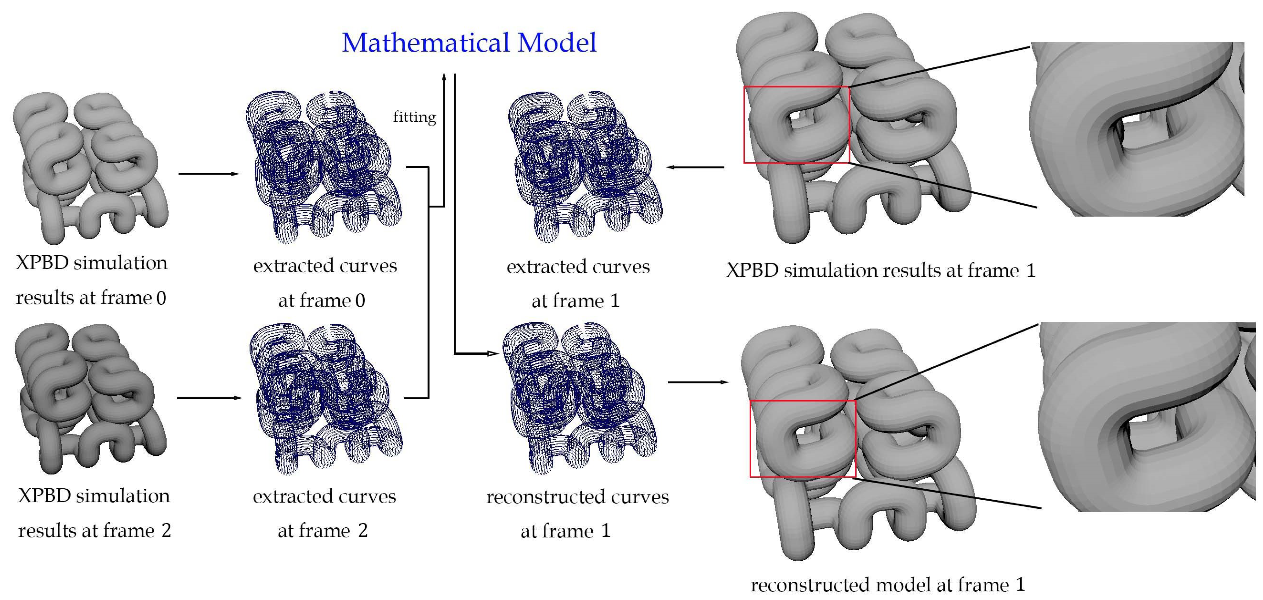
4. PDE-Based Dynamic Reconstruction

Dynamic simulation involves heavy numerical calculations. Usually, the whole simulation is divided into some time steps. Small time steps greatly increase computational time, leading to low efficiency of the computer animation. Large time steps make some temporal details disappear and further decrease the numerical stability. In this section, we investigate a dynamic PDE-based algorithm, which can be combined with numerical methods such as XPBD to enable large time steps while keeping temporal details.

The extended position-based dynamics algorithm is based on Newton’s equation of motion, in which the deformation force is replaced by the gradient of an energy potential defined with a vector consisting of constraint functions. Since the constraint functions are not directly related to the underlying deformation physics, we first modify it to include the underlying deformation physics.

4.1. Mathematical Model

A surface can be defined by a vector-valued function $\mathbf{S}(u,v)$, where u and v are two parametric variables. When the parametric variable v takes a certain value $v_0$, the vector-valued function $\mathbf{S}(u,v_0)$ defines a curve. Therefore, the surface $\mathbf{S}(u,v)$ can be regarded as a sweeping surface obtained by sweeping the curve $\mathbf{S}(u,v_0)$.

The deformation of a curve is similar to the deformation of an elastic beam, which is defined by the following equation:

$$K{\displaystyle \frac{d^{4}w}{d{l}^4}}=q,$$

(8)

where K is the flexural rigidity of the elastic beam, w is the lateral deformation, l is the length variable of the elastic beam, and q is an external force.

When Equation (1) is used to describe dynamic deformation of an elastic beam, the position vector $\mathbf{x}$ in Equation (1) becomes the lateral deformation w. From Equation (8), we know that the deformation force for an elastic beam is $K{d}^{4}w/d{l}^4$. Using it to replace the right term of Equation (1) and mass m to replace the mass matrix $\mathbf{M}$ and noticing that the position vector $\mathbf{x}$ becomes w and $\ddot{\mathbf{x}}$ becomes $d^{2}w/d{t}^2$, we obtain the following equation, which describes the underlying deformation physics:

$$m{\displaystyle \frac{d^{2}w}{d{t}^2}}=K{\displaystyle \frac{d^{4}w}{d{l}^4}}.$$

(9)

When using the above equation to describe the deformation of a 3D curve, w becomes three position components x, y, and z, and the length variable l becomes the parametric variable u, and Equation (9) is changed into

$$m{\displaystyle \frac{d^{2}w}{d{t}^2}}=K{\displaystyle \frac{d^{4}w}{d{u}^4}}(w=x,y,z),$$

(10)

where $w=w(u,t)$ is the function of the parametric variable u and the time variable t.

The partial differential equations in the above Equation (10) present the mathematical model we build to represent the dynamic deformation of the curves defining a surface model. They consider both the time variable t and the parametric variable u so that they can be used to simulate the dynamic deformation of a curve at different time t.

Although metaheuristic algorithms such as [49,50,51] have been proposed to solve complex or non-linear partial differential equations and optimization problems, they cannot give exact solutions and are computationally intensive and sensitive to the initial conditions. In contrast, closed-form solutions have the advantages of exactness, efficiency, robustness, ease of interpretation, etc. In what follows, we investigate the closed-form solutions of Equation (10).

4.2. The Closed-Form Solutions

Equation (10) contains the fourth derivative of w with respect to the parametric variable u. To satisfy Equation (10), the fourth derivative of w with respect to the parametric variable u must be w multiplied by a coefficient. Thus, w can be constructed as $e^{ru}\overline{w}\left(t\right)$.

Substituting $w=e^{ru}\overline{w}\left(t\right)$ into Equation (10) and eliminating $e^{ru}$, Equation (10) is changed into the following second-order ordinary differential equation:

$$m{\overline{w}}^{\prime \prime }\left(t\right)=K{r}^4\overline{w}\left(t\right).$$

(11)

Solving the above second-order ordinary differential equation, we obtain its closed-form solutions, which include the following elementary functions:

$$e^{\alpha t},e^{-\alpha t},sin\left(\alpha t\right),cos\left(\alpha t\right),$$

(12)

where $\alpha =r^2\sqrt{k/m}$.

Having known the elementary functions of the time variable t, we can construct w as $e^{\alpha t}\tilde{w}\left(u\right)$, $e^{-\alpha t}\tilde{w}\left(u\right)$, $sin\left(\alpha t\right)\tilde{w}\left(u\right)$, and $cos\left(\alpha t\right)\tilde{w}\left(u\right)$.

Substituting $w=e^{\alpha t}\tilde{w}\left(u\right)$ into Equation (10) and eliminating $e^{\alpha t}$, Equation (10) is changed into the following fourth-order ordinary differential equation:

$$m{\alpha }^2\tilde{w}\left(u\right)=K{\tilde{w}}^{\prime \prime \prime \prime }\left(u\right).$$

(13)

Solving the above fourth-order ordinary differential equation of the parametric variable u, we obtain its closed-form solutions, which include the following elementary functions:

$$e^{ru},e^{-ru},sin\left(ru\right),cos\left(ru\right).$$

(14)

Similarly, by substituting $w=e^{-\alpha t}\tilde{w}\left(u\right)$ into Equation (10) and eliminating $e^{-\alpha t}$, we can obtain the second-order ordinary differential Equation (13) and the elementary functions same as those in Equation (14).

Substituting $w=sin\left(\alpha t\right)\tilde{w}\left(u\right)$ into Equation (10) and eliminating $sin\left(\alpha t\right)$, Equation (10) is changed into the following fourth-order ordinary differential equation:

$$-m{\alpha }^2\tilde{w}\left(u\right)=K{\tilde{w}}^{\prime \prime \prime \prime }\left(u\right).$$

(15)

Solving the above fourth-order ordinary differential equation of the parametric variable u, we obtain its closed-form solutions, which include the following elementary functions:

$$e^{\overline{r}u}sin\left(\overline{r}u\right),e^{\overline{r}u}cos\left(\overline{r}u\right),e^{-\overline{r}u}sin\left(\overline{r}u\right),e^{-\overline{r}u}cos\left(\overline{r}u\right),$$

(16)

where $\overline{r}=\sqrt{2}r/2$.

Similarly, by substituting $w=cos\left(\alpha t\right)\tilde{w}\left(u\right)$ into Equation (10) and eliminating $cos\left(\alpha t\right)$, we can obtain the fourth-order ordinary differential Equation (15) and the elementary functions that are the same as those in Equation (16).

In order to make the solution to Equation (10) have enough unknown constants to well reconstruct time-dependent dynamic deformation curves, we use all the elementary functions in Equations (12), (14) and (16) to construct the solution. Multiplying each of the elementary functions in Equations (14) and (16) by each of the elementary functions in Equation (12) and introducing the unknown constants $c_{wn}$ to produce a linear combination of the multiplication result, we obtain the following solution to Equation (10):

$$w(u,t)=\sum _{n=1}^{32}{c}_{wn}{w}_n(u,t,\alpha ,r,\overline{r}),$$

(17)

where $w_n(u,t,\alpha ,r,\overline{r})(n=1,2,\cdots ,32)$ are

$$\begin{array}{cccc}\hfill w_1(u,t,\alpha ,r,\overline{r})& =e^{\alpha t}{e}^{ru},\hfill & \hfill w_2(u,t,\alpha ,r,\overline{r})& =e^{\alpha t}{e}^{-ru},\hfill \\ \hfill w_3(u,t,\alpha ,r,\overline{r})& =e^{\alpha t}sin\left(ru\right),\hfill & \hfill w_4(u,t,\alpha ,r,\overline{r})& =e^{\alpha t}cos\left(ru\right),\hfill \\ \hfill w_5(u,t,\alpha ,r,\overline{r})& =e^{\alpha t}{e}^{\overline{r}u}sin\left(\overline{r}u\right),\hfill & \hfill w_6(u,t,\alpha ,r,\overline{r})& =e^{\alpha t}{e}^{\overline{r}u}cos\left(\overline{r}u\right),\hfill \\ \hfill w_7(u,t,\alpha ,r,\overline{r})& =e^{\alpha t}{e}^{-\overline{r}u}sin\left(\overline{r}u\right),\hfill & \hfill w_8(u,t,\alpha ,r,\overline{r})& =e^{\alpha t}{e}^{-\overline{r}u}cos\left(\overline{r}u\right),\hfill \\ \hfill w_9(u,t,\alpha ,r,\overline{r})& =e^{-\alpha t}{e}^{ru},\hfill & \hfill w_{10}(u,t,\alpha ,r,\overline{r})& =e^{-\alpha t}{e}^{-ru},\hfill \\ \hfill w_{11}(u,t,\alpha ,r,\overline{r})& =e^{-\alpha t}sin\left(ru\right),\hfill & \hfill w_{12}(u,t,\alpha ,r,\overline{r})& =e^{-\alpha t}cos\left(ru\right),\hfill \\ \hfill w_{13}(u,t,\alpha ,r,\overline{r})& =e^{-\alpha t}{e}^{\overline{r}u}sin\left(\overline{r}u\right),\hfill & \hfill w_{14}(u,t,\alpha ,r,\overline{r})& =e^{-\alpha t}{e}^{\overline{r}u}cos\left(\overline{r}u\right),\hfill \\ \hfill w_{15}(u,t,\alpha ,r,\overline{r})& =e^{-\alpha t}{e}^{-\overline{r}u}sin\left(\overline{r}u\right),\hfill & \hfill w_{16}(u,t,\alpha ,r,\overline{r})& =e^{-\alpha t}{e}^{-\overline{r}u}cos\left(\overline{r}u\right),\hfill \\ \hfill w_{17}(u,t,\alpha ,r,\overline{r})& =sin\left(\alpha t\right)e^{ru},\hfill & \hfill w_{18}(u,t,\alpha ,r,\overline{r})& =sin\left(\alpha t\right)e^{-ru},\hfill \\ \hfill w_{19}(u,t,\alpha ,r,\overline{r})& =sin\left(\alpha t\right)sin\left(ru\right),\hfill & \hfill w_{20}(u,t,\alpha ,r,\overline{r})& =sin\left(\alpha t\right)cos\left(ru\right),\hfill \\ \hfill w_{21}(u,t,\alpha ,r,\overline{r})& =sin\left(\alpha t\right)e^{\overline{r}u}sin\left(\overline{r}u\right),\hfill & \hfill w_{22}(u,t,\alpha ,r,\overline{r})& =sin\left(\alpha t\right)e^{\overline{r}u}cos\left(\overline{r}u\right),\hfill \\ \hfill w_{23}(u,t,\alpha ,r,\overline{r})& =sin\left(\alpha t\right)e^{-\overline{r}u}sin\left(\overline{r}u\right),\hfill & \hfill w_{24}(u,t,\alpha ,r,\overline{r})& =sin\left(\alpha t\right)e^{-\overline{r}u}cos\left(\overline{r}u\right),\hfill \\ \hfill w_{25}(u,t,\alpha ,r,\overline{r})& =cos\left(\alpha t\right)e^{ru},\hfill & \hfill w_{26}(u,t,\alpha ,r,\overline{r})& =cos\left(\alpha t\right)e^{-ru},\hfill \\ \hfill w_{27}(u,t,\alpha ,r,\overline{r})& =cos\left(\alpha t\right)sin\left(ru\right),\hfill & \hfill w_{28}(u,t,\alpha ,r,\overline{r})& =cos\left(\alpha t\right)cos\left(ru\right),\hfill \\ \hfill w_{29}(u,t,\alpha ,r,\overline{r})& =cos\left(\alpha t\right)e^{\overline{r}u}sin\left(\overline{r}u\right),\hfill & \hfill w_{30}(u,t,\alpha ,r,\overline{r})& =cos\left(\alpha t\right)e^{\overline{r}u}cos\left(\overline{r}u\right),\hfill \\ \hfill w_{31}(u,t,\alpha ,r,\overline{r})& =cos\left(\alpha t\right)e^{-\overline{r}u}sin\left(\overline{r}u\right),\hfill & \hfill w_{32}(u,t,\alpha ,r,\overline{r})& =cos\left(\alpha t\right)e^{-\overline{r}u}cos\left(\overline{r}u\right).\hfill \end{array}$$

(18)

4.3. Transformation Elimination

After the reconstruction function has been constructed, the remaining tasks are to solve the unknown integration constants in Equation (17) and then use it to create new deformation shapes.

Assuming the deformation shapes of a 3D model at frame $n(n=0,1,\dots ,N)$ are known and the time corresponds to frame n is $t_n$, we use $w_{nk}(w=x,y,z)$ to indicate the x, y, and z coordinate values of the $k^{th}$ point $(k=1,2,3,\dots ,K)$ on one of the curves defining a 3D model at frame n.

When a 3D model moves from one frame to the next frame, rigid transformations may be involved. We remove rigid transformations through the following treatment.

First, we align the first point of a curve at different frames through

$$\begin{array}{cc}\hfill {\overline{w}}_{nk}& =w_{nk}-(w_{n0}-w_{00}).\hfill \\ \hfill (w=x,y,z;n& =1,2,\dots ,N;k=1,2,\dots ,K)\hfill \end{array}$$

(19)

After that, we rotate the curve at frame n to align with the curve at frame 0. If the curve at frame 0 is defined by the points ${\tilde{\mathbf{x}}}_{0k}={\left[\begin{array}{ccc}{\tilde{x}}_{0k}& {\tilde{y}}_{0k}& {\tilde{z}}_{0k}\end{array}\right]}^T$$(k=1,2,\dots ,K)$ and the curve at frame n after rotation is defined by the points ${\tilde{\mathbf{x}}}_{nk}={\left[\begin{array}{ccc}{\tilde{x}}_{nk}& {\tilde{y}}_{nk}& {\tilde{z}}_{nk}\end{array}\right]}^T$$(k=1,2,\dots ,K)$, we minimize the sum of the distance between the points ${\tilde{\mathbf{x}}}_{nk}$ and the points ${\tilde{\mathbf{x}}}_{0k}$ to find the rotation matrix.

For a rotation in 3D, the general rotation matrix at frame n can be formulated as

$$\left[\begin{array}{ccc}{a}_{n,11}& a_{n,12}& a_{n,13}\\ a_{n,21}& a_{n,22}& a_{n,23}\\ a_{n,31}& a_{n,32}& a_{n,33}\end{array}\right].$$

(20)

Using the above rotation matrix to align the curve at frame n to the curve at frame 0 means the following matrix multiplication:

$$\left[\begin{array}{ccc}{\overline{x}}_{nk}& {\overline{y}}_{nk}& {\overline{z}}_{nk}\end{array}\right]\left[\begin{array}{ccc}{a}_{n,11}& a_{n,12}& a_{n,13}\\ a_{n,21}& a_{n,22}& a_{n,23}\\ a_{n,31}& a_{n,32}& a_{n,33}\end{array}\right],$$

(21)

which changes the curve point ${\overline{w}}_{nk}$ into ${\tilde{w}}_{nk}$ below:

$$\begin{array}{cc}\hfill {\tilde{x}}_{nk}& =a_{n,11}{\overline{x}}_{nk}+a_{n,21}{\overline{y}}_{nk}+a_{n,31}{\overline{z}}_{nk},\hfill \\ \hfill {\tilde{y}}_{nk}& =a_{n,12}{\overline{x}}_{nk}+a_{n,22}{\overline{y}}_{nk}+a_{n,32}{\overline{z}}_{nk},\hfill \\ \hfill {\tilde{z}}_{nk}& =a_{n,13}{\overline{x}}_{nk}+a_{n,23}{\overline{y}}_{nk}+a_{n,33}{\overline{z}}_{nk}.\hfill \end{array}$$

(22)

The elements $a_{i,j}(i,j=1,2,3)$ in the rotation matrix are obtained by minimizing the sum of the squared errors between the points ${\tilde{w}}_{nk}$ and $w_{0k}$, i.e.,

$$\begin{array}{cc}\hfill {\displaystyle \frac{\partial }{\partial a_{n,rs}}}\sum _{k=1}^K\left[\right({\tilde{x}}_{nk}& -{\overline{x}}_{0k}{)}^2+{({\tilde{y}}_{0k}-{\overline{y}}_{0k})}^2+{({\tilde{z}}_{0k}-{\overline{z}}_{0k})}^2]=0.\hfill \\ \hfill (n& =1,2,\dots ,N;r,s=1,2,3)\hfill \end{array}$$

(23)

After all the elements in the rotation matrix are determined, we use Equation (22) to obtain ${\tilde{w}}_{nk}$.

4.4. Parametrization

In order to approximate the curve at frame n with Equation (17), we should first determine the values of the parametric variable u. To do this, we find the minimum and maximum values of ${\tilde{w}}_{nk}$ and denote them with ${\tilde{w}}_{n,min}$ and ${\tilde{w}}_{n,max}$, respectively. The u parametric value corresponding to the $k^{th}$ point at frame n is obtained as

$$u_{nk}={\displaystyle \frac{{\tilde{w}}_{nk}-{\tilde{w}}_{n,min}}{{\tilde{w}}_{n,max}-{\tilde{w}}_{n,min}}}.$$

(24)

4.5. Unknown Constants Determination

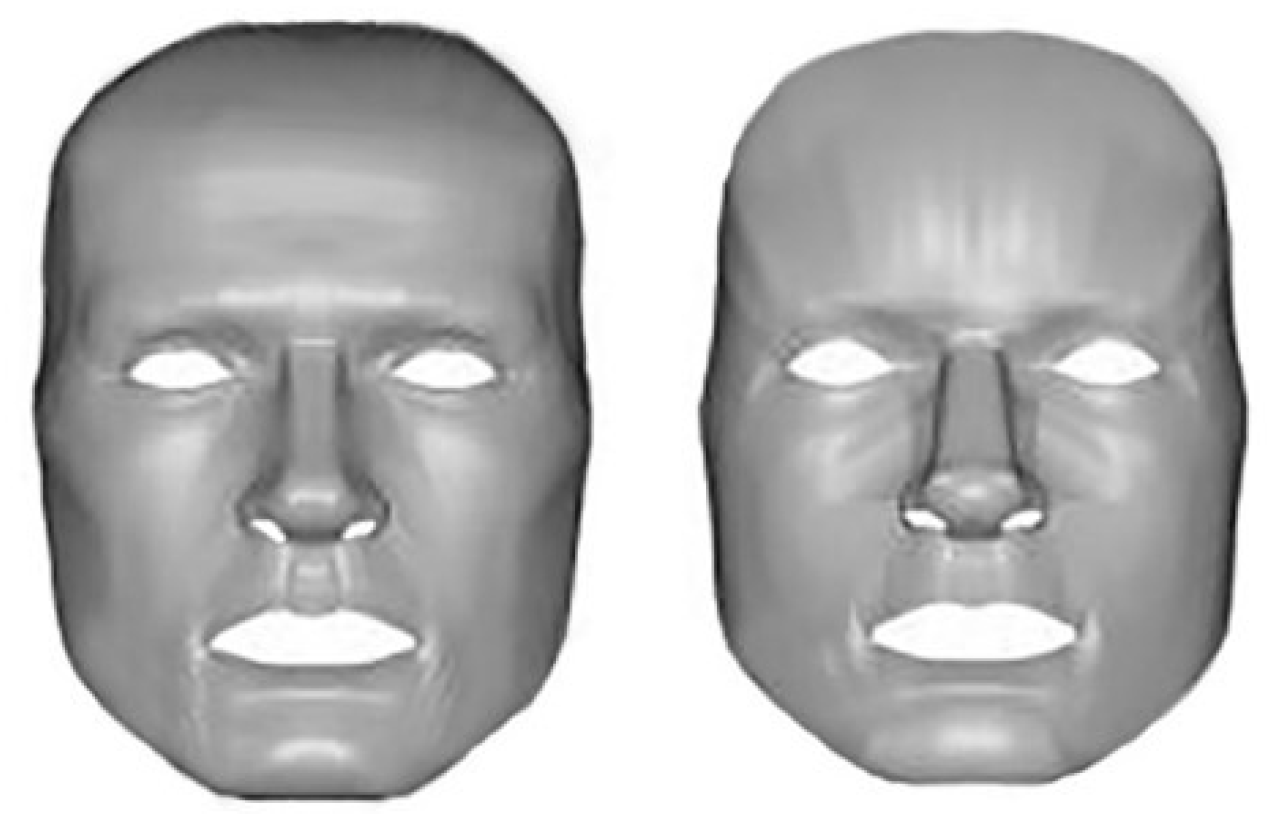
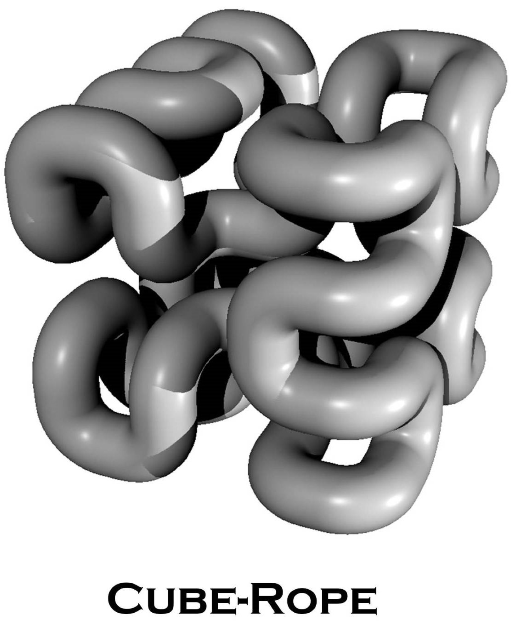
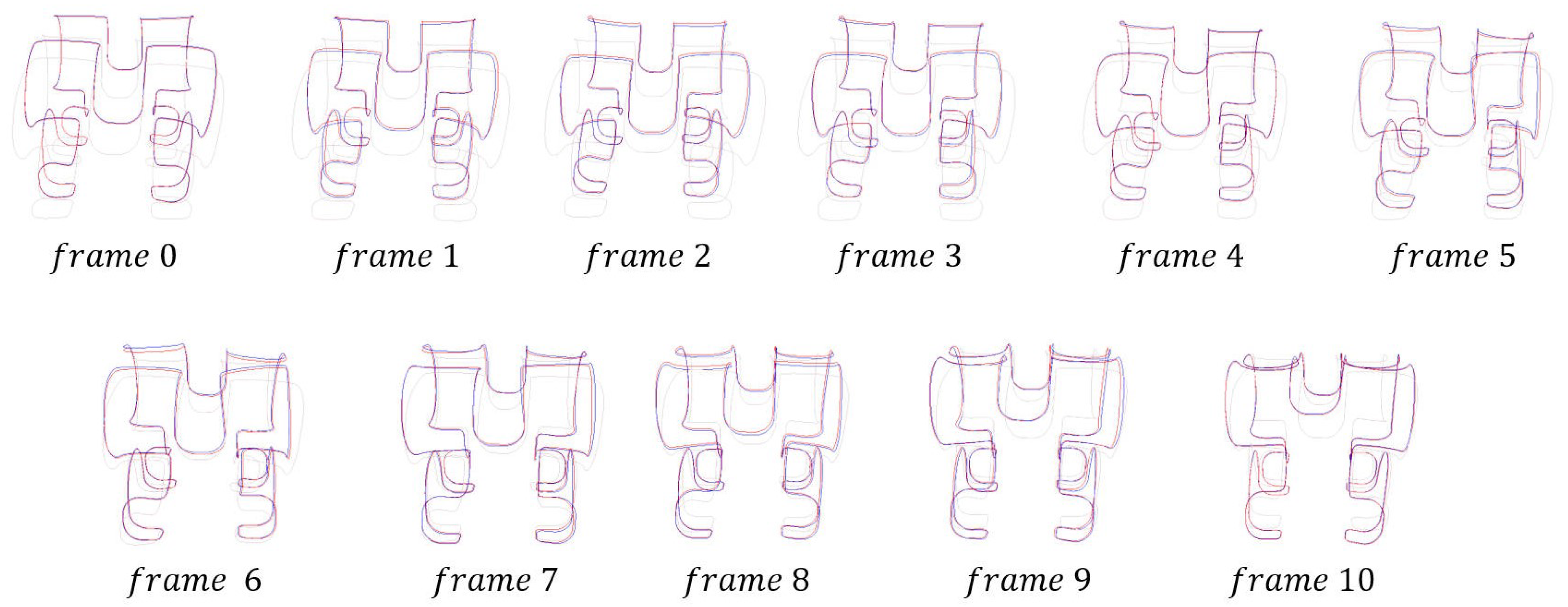
Substituting $t_n$ and $u_{nk}$ into Equation (17), we obtain the predicted values $w(u_{nk},t_n)$. We calculate the sum of the squared errors between the predicted values $w(u_{nk},t_n)$ and real values ${\tilde{w}}_{nk}$ for all the points on the curve for all the frames and minimizing the sum to determine the unknown integration constants involved in Equation (17), i.e.,

$$\begin{array}{cc}\hfill & {\displaystyle \frac{\partial }{\partial c_{wm}}}\sum _{n=0}^N\sum _{k=1}^K{[w(u_{nk},t_n)-{\tilde{w}}_{nk}]}^2\hfill \\ \hfill =& {\displaystyle \frac{\partial }{\partial c_{wm}}}\sum _{n=0}^N\sum _{k=1}^K{[\sum _{i=1}^{32}{c}_{wi}{w}_i(u_{nk},t_n,\alpha ,r,\overline{r})-{\tilde{w}}_{nk}]}^2=0.\hfill \\ & (w=x,y,z;m=1,2,\dots ,32)\hfill \end{array}$$

(25)

By solving the 32 linear equations in Equation (25), we determine the 32 unknown integration constants. Substituting them back into Equation (17), we use it to create new deformed shapes of the 3D models at new frames. In the following section, we will give an example to demonstrate the application of Equation (17) in dynamic reconstruction.

5. Experiment

The algorithm presented in the above section is implemented with C++, where the implemented computer program is run on the platform Visual Studio 2022. The cube-rope model that we use to illustrate our proposed PDE-based dynamic reconstruction is provided by Zhou et al. in [52].

In order to use the proposed algorithm to reconstruct the deformed shapes, we convert the surface-represented 3D model shown in Figure 3 into a curve-represented model. We manually extract curves along the length direction of the cube-rope model. The cube-rope model is defined by 19,968 vertices. In total, 24 curves are extracted, and each curve has 832 points. Figure 4 shows the curve-represented models at the 10 frames: $0,1,\dots ,9$. Each extracted curve is then used to fit the proposed mathematical model and recreated by the method presented in Section 4. Finally, all the curves are used to reconstruct the cube-rope models. The whole framework is shown in Figure 5 for a better understanding.

For the purpose of illustration, we take the 1st extracted curve to demonstrate the dynamic reconstruction process. The same method is applicable to the remaining 23 extracted curves.

As discussed in Section 4, we first align the first point of the 1st curve at frame 1 to frame 10 with the first point of the 1st curve at frame 0 through Equation (19) and obtain ${\overline{w}}_{nk}(n=1,2,\dots ,10;k=1,2,\dots ,832)$. Then, we solve Equation (23) to determine the elements of the rotation matrix, and use Equation (22) to obtain ${\tilde{w}}_{nk}(n=1,2,\dots ,10;k=1,2,\dots ,832)$. After that, we use the deformed shapes at frames 0, 2, 4, 6, 8, and 10 and Equation (25) to determine the unknown constants $c_{wn}$ in Equation (17). In order to generate deformation shapes at frames 1, 3, 5, 7, and 9, we determine $u_{nk}(w=x,y,z;n=1,3,5,7,9;k=1,2,\dots ,832)$ at frames 1, 3, 5, 7, and 9, use Equation (17) to calculate the deformed shapes at frames $0,1,2,3,\dots ,10$, and depict them as red curves in Figure 6, where the baseline curves are in blue.

For the static reconstruction with B-Spline curves and linear interpolation called static B-Spline curve-based linear interpolation, we use cubic B-Spline curves with 50 control points each provided in [53] to fit the model and obtain B-Spline curves at frames 0, 2, 4, 6, 8, and 10. Then, we linearly interpolate two adjacent B-Spline curves at frames 0, 2, 4, 6, 8, and 10 to obtain the B-Spline curves at frames 1, 3, 5, 7, and 9, and depict B-Spline curves at frame $0,1,2,3,\dots ,10$ as light green curves in Figure 6 as well.

After that, we use the reconstructed B-Spline curves at frames 0, 2, 4, 6, 8, and 10 and the interpolated B-Spline curves at frames 1, 3, 5, 7, and 9 to calculate the coordinate values $w_{nk}(w=x,y,z;n=0,1,\dots ,10;k=1,2,\dots ,832)$. Then, we quantify the errors between the baseline shapes ${\tilde{w}}_{nk}$ and the reconstructed shapes obtained from our proposed PDE-based dynamic reconstruction algorithm and the static B-Spline curve-based reconstruction method through the following Equation (26) to calculate the average error:

$$E_{An}={\displaystyle \frac{1}{832D}}\sum _{k=0}^{832}∥{\tilde{w}}_{nk}-{\widehat{w}}_{nk}∥(n=0,1,2,\dots ,10),$$

(26)

and Equation (27) to calculate the maximum error:

$$E_{Mn}={\displaystyle \frac{1}{D}}max\left\{∥{\tilde{w}}_{nk}-{\widehat{w}}_{nk}∥\right\}(n=0,1,2,\dots ,10;k=1,2,\dots ,832),$$

(27)

where $E_{An}$ is the average error, ${\widehat{w}}_{nk}=w(u_{nk},t_n)$ for the PDE-based dynamic reconstruction, ${\widehat{w}}_{nk}=w\left(u_{nk}\right)$ for the static B-Spline curve-based reconstruction, $E_{Mn}$ is the maximum error, and D is the distance between the two furthest points of the 1st extracted curve.

With Equations (26) and (27), we obtain the average errors and maximum errors between the baseline shapes and the deformed shapes reconstructed with the developed PDE-based dynamic reconstruction algorithm and between the baseline shapes and deformed shapes reconstructed with the static B-spline curve-based reconstruction method. These errors are given in

Table 1. Average errors and maximum errors of our proposed PDE-based dynamic reconstruction algorithm and static B-Spline curve-based linear interpolation method compared with XPBD results.

	PDE		B-Spline
Frame	${\mathit{E}}_{\mathit{An}}$	${\mathit{E}}_{\mathit{Mn}}$	${\mathit{E}}_{\mathit{An}}$	${\mathit{E}}_{\mathit{Mn}}$
0	0.003035	0.005387	0.009169	0.110480
1	0.007886	0.017251	0.054134	0.187488
2	0.009044	0.014629	0.090012	0.111336
3	0.008655	0.019478	0.077795	0.143668
4	0.005158	0.008127	0.024759	0.2525
5	0.007315	0.01675	0.062312	0.199951
6	0.007807	0.018031	0.035425	0.245637
7	0.006296	0.013386	0.034231	0.106627
8	0.010102	0.016598	0.037255	0.181635
9	0.008118	0.016756	0.055076	0.169511
10	0.003429	0.015639	0.032914	0.270942

.

We can observe from Figure 6 that the reconstructed curves from our proposed dynamic PDE-based reconstruction algorithm exhibit minimal differences with the baseline curves generated by XPBD, except for some parts when the curvature fluctuates. Conversely, the curves produced by the static B-Spline curve-based linear interpolation method display noticeable deviations from the baseline curves. This observation is supported by the average and maximum errors presented in Table 1. Compared with the deformed shapes of the cube-rope model obtained with XPBD simulation, the mean value of the average errors $E_{An}$ and the maximum value of the maximum errors $E_{Mn}$ of our proposed PDE-based dynamic reconstruction method are $0.006986$ and $0.019478$, respectively, whilst those of the static B-Spline curve-based linear interpolation method are $0.046644$ and $0.270942$. The accuracy improvement is obvious. The mean value of the average errors from the static B-Spline curve-based linear interpolation method is $6.68$ times the mean value of the average errors from our proposed PDE-based dynamic reconstruction algorithm, and the maximum value of the maximum errors from the static B-Spline curve-based linear interpolation is $13.91$ times the maximum value of the maximum errors from our proposed PDE-based dynamic reconstruction algorithm.

With the XPBD algorithm, the CPU time used to generate the 11 frames is $7.442$ s and that for frames 0, 2, 4, 6, 8, and 10 is $4.085$ s for the cube-rope model. Using frames 0, 2, 4, 6, 8, and 10 to determine the unknown constants in Equation (17) and generating reconstructed shapes at frame 1, 3, 5, 7, and 9 with Equation (17), it is $0.293$ s. Using frame 0, 2, 4, 6, 8, and 10 to determine the unknown control points in the B-Spline curves for reconstructing B-Spline curves at frames 0, 2, 4, 6, 8, and 10 and linearly interpolating the reconstructed B-Spline curves to obtain B-Spline curves at frame 1, 3, 5, 7 and 9, it is $0.034$ s. In addition to the $4.085$ s used by XPBD to generate frames 0, 2, 4, 6, 8, and 10, our proposed PDE-based dynamic reconstruction algorithm takes $4.378$ s to generate the shapes at the 11 frames (frame 0 to frame 10), and the static B-Spline curve-based linear interpolation method take $4.119$ s to generate the shapes at the 11 frames. The above data show that our proposed PDE-based dynamic reconstruction algorithm combined with the XPBD simulation only requires $58.13\%$ of the time required by XPBD to generate the shapes at the 11 frames. It indicates that combining XPBD simulation with our proposed PDE-based dynamic reconstruction nearly doubles the simulation efficiency. Although the total time required by our proposed PDE-based dynamic reconstruction algorithm is a little more than the total time required by the static B-Spline curve-based linear interpolation, our proposed PDE-based dynamic reconstruction algorithm has higher accuracy, involves fewer design variables, and is physics based.

In addition to the above error and efficiency comparisons, here, we compare the number of design variables among the three different methods. With the XPBD, the cube-rope model at each of the 11 frames is defined by 19,968 vertices (design variables). In total, 219,648 design variables are required to define the cube-rope model at the 11 frames $0,1,2,\dots ,9,10$. With the static B-spline curve-based linear interpolation method, 50 control points (design variables) are used to define one of the 24 curves representing the cube-rope model, which means that 1200 design variables are used to define the cube-rope model at each of the six frames 0, 2, 4, 6, 8, and 10. The cube-rope model at frames 1, 3, 5, 7, and 9 is obtained by linearly interpolating the frames 0, 2, 4, 6, 8, and 10. In total, 7200 design variables are required to define the cube-rope model at the 11 frames. With our proposed PDE-based dynamic reconstruction method, 32 unknown constants (design variables) in Equation (17) are used to define one of the 24 curves representing the cube-rope model. In total, 768 design variables are used to define the cube-rope model. Once the 768 design variables are obtained, the cube-rope model at the 11 frames $0,1,2,\dots ,9,10$ is determined by setting the time variable t in Equation (17) to $0.0,0.1,\dots ,1.0$. In comparison with the 219,648 design variables required by the XPBD algorithm and 7200 design variables required by the static B-spline curve-based linear interpolation, the design variables required by our proposed PDE-based dynamic reconstruction method are only $0.35\%$ and $10.67\%$ required by the XPBD algorithm and the static B-spline curve-based linear interpolation.

The above discussions indicate that our proposed PDE-based dynamic reconstruction algorithm can effectively reconstruct the XPBD simulated deformed shapes with good accuracy and high efficiency while using fewer design variables. It is advantageous compared to the static B-spline curve-based representation and linear interpolation.

6. Conclusions

In this paper, we have proposed a physics-based dynamic reconstruction and interpolation method of dynamic deformation simulation. To this end, we first converted surface-represented 3D models into curve-represented 3D models. Then, we presented a mathematical model of PDE-based dynamic reconstruction by replacing the deformation forces derived from the XPBD constraint function with elastic beam bending forces. Finally, we developed a compact and analytical solution of the mathematical model and combined it with XPBD to obtain a quick and accurate reconstruction of XPBD simulation with far smaller data sizes.

We have conducted an experiment to validate the developed PDE-based dynamic reconstruction algorithm. The experimental results demonstrate that our algorithm significantly reduces design variables and greatly shortens simulation time compared to XPBD while maintaining high reconstruction accuracy. The comparison with static B-Spline curve-based representation and linear interpolation indicates that the developed PDE-based reconstruction has higher reconstruction accuracy and smaller data sizes. Unlike XPBD simulation, which obtains deformed shapes at discrete frames, the developed PDE-based dynamic reconstruction can be used to create continuous deformed shapes, thus raising the deformation simulation capacity.

References

1. Daniels, J.; Silva, C.T.; Shepherd, J.; Cohen, E. Quadrilateral mesh simplification. ACM Trans. Graph. (TOG) 2008, 27, 1–9. [Google Scholar] [CrossRef]
2. Ebke, H.C.; Campen, M.; Bommes, D.; Kobbelt, L. Level-of-detail quad meshing. ACM Trans. Graph. (TOG) 2014, 33, 1–11. [Google Scholar] [CrossRef]
3. Magnenat, T.; Laperrière, R.; Thalmann, D. Joint-Dependent Local Deformations for Hand Animation and Object Grasping; Technical Report; Canadian Information Processing Society: Mississauga, ON, Canada, 1988. [Google Scholar]
4. Alexa, M. Linear combination of transformations. ACM Trans. Graph. (TOG) 2002, 21, 380–387. [Google Scholar] [CrossRef]
5. Magnenat-Thalmann, N.; Cordier, F.; Seo, H.; Papagianakis, G. Modeling of bodies and clothes for virtual environments. In Proceedings of the 2004 International Conference on Cyberworlds, Tokyo, Japan, 18–20 November 2004; IEEE: Piscataway, NJ, USA, 2004; pp. 201–208. [Google Scholar]
6. Kavan, L.; Žára, J. Spherical blend skinning: A real-time deformation of articulated models. In Proceedings of the 2005 Symposium on Interactive 3D Graphics and Games, Washington, DC, USA, 3–5 April 2005; pp. 9–16. [Google Scholar]
7. Kavan, L.; Collins, S.; Žára, J.; O’Sullivan, C. Geometric skinning with approximate dual quaternion blending. ACM Trans. Graph. (TOG) 2008, 27, 1–23. [Google Scholar] [CrossRef]
8. Mancewicz, J.; Derksen, M.L.; Rijpkema, H.; Wilson, C.A. Delta mush: Smoothing deformations while preserving detail. In Proceedings of the Fourth Symposium on Digital Production, Vancouver, BC, Canada, 9 August 2014; pp. 7–11. [Google Scholar]
9. Le, B.H.; Lewis, J. Direct delta mush skinning and variants. ACM Trans. Graph. 2019, 38, 113:1–113:13. [Google Scholar] [CrossRef]
10. Sederberg, T.W.; Parry, S.R. Free-form deformation of solid geometric models. In Proceedings of the 13th Annual Conference on Computer Graphics and Interactive Techniques, Dallas, TX, USA, 18–22 August 1986; pp. 151–160. [Google Scholar]
11. Coquillart, S. Extended free-form deformation: A sculpturing tool for 3D geometric modeling. In Proceedings of the 17th Annual Conference on Computer Graphics and Interactive Techniques, Dallas, TX, USA, 6–10 August 1990; pp. 187–196. [Google Scholar]
12. Coquillart, S.; Jancene, P. Animated free-form deformation: An interactive animation technique. ACM Siggraph Comput. Graph. 1991, 25, 23–26. [Google Scholar] [CrossRef]
13. Schein, S.; Elber, G. Discontinuous free form deformations. In Proceedings of the 12th Pacific Conference on Computer Graphics and Applications, 2004, PG 2004, Proceedings, Seoul, Republic of Korea, 6–8 October 2004; IEEE: Piscataway, NJ, USA, 2004; pp. 227–236. [Google Scholar]
14. Etzmuss, O.; Gross, J.; Strasser, W. Deriving a particle system from continuum mechanics for the animation of deformable objects. IEEE Trans. Vis. Comput. Graph. 2003, 9, 538–550. [Google Scholar] [CrossRef]
15. Desbrun, M.; Schröder, P.; Barr, A. Interactive animation of structured deformable objects. Graph. Interface 1999, 99, 10. [Google Scholar]
16. Zienkiewicz, O.C.; Taylor, R.L.; Zhu, J.Z. The Finite Element Method: Its Basis and Fundamentals; Elsevier: Amsterdam, The Netherlands, 2005. [Google Scholar]
17. Patidar, K.C. On the use of nonstandard finite difference methods. J. Differ. Equations Appl. 2005, 11, 735–758. [Google Scholar] [CrossRef]
18. James, D.L.; Pai, D.K. Artdefo: Accurate real time deformable objects. In Proceedings of the 26th Annual Conference on Computer Graphics and Interactive Techniques, Los Angeles, CA, USA, 8–13 August 1999; pp. 65–72. [Google Scholar]
19. Teran, J.; Blemker, S.; Ng-Thow-Hing, V.; Fedkiw, R. Finite volume methods for the simulation of skeletal muscle. In Proceedings of the 2003 ACM SIGGRAPH/Eurographics symposium on Computer Animation, San Diego, CA, USA, 26–27 July 2003; pp. 68–74. [Google Scholar]
20. Yousefi, M.; Pervaiz, S. 3D Finite element modeling of wear effects in the punching process. Simul. Model. Pract. Theory 2022, 114, 102415. [Google Scholar] [CrossRef]
21. Pressas, I.S.; Papaefthymiou, S.; Manolakos, D.E. Evaluation of the roll elastic deformation and thermal expansion effects on the dimensional precision of flat ring rolling products: A numerical investigation. Simul. Model. Pract. Theory 2022, 117, 102499. [Google Scholar] [CrossRef]
22. Allen, B.; Curless, B.; Popović, Z. Articulated body deformation from range scan data. ACM Trans. Graph. (TOG) 2002, 21, 612–619. [Google Scholar] [CrossRef]
23. Anguelov, D.; Srinivasan, P.; Koller, D.; Thrun, S.; Rodgers, J.; Davis, J. SCAPE: Shape completion and animation of people. ACM Trans. Graph. 2005, 24, 408–416. [Google Scholar] [CrossRef]
24. Der, K.G.; Sumner, R.W.; Popović, J. Inverse kinematics for reduced deformable models. ACM Trans. Graph. (TOG) 2006, 25, 1174–1179. [Google Scholar] [CrossRef]
25. Müller, M.; Heidelberger, B.; Hennix, M.; Ratcliff, J. Position based dynamics. J. Vis. Commun. Image Represent. 2007, 18, 109–118. [Google Scholar] [CrossRef]
26. Müller, M. Hierarchical Position Based Dynamics. In Proceedings of the 2008 Workshop in Virtual Reality Interactions and Physical Simulation, Grenoble, France, 13–14 November 2008; Volume 8, pp. 1–10. [Google Scholar]
27. Müller, M.; Keiser, R.; Nealen, A.; Pauly, M.; Gross, M.; Alexa, M. Point based animation of elastic, plastic and melting objects. In Proceedings of the 2004 ACM SIGGRAPH/Eurographics Symposium on Computer Animation, Grenoble France, 27–29 August 2004; pp. 141–151. [Google Scholar]
28. Bouaziz, S.; Martin, S.; Liu, T.; Kavan, L.; Pauly, M. Projective dynamics: Fusing constraint projections for fast simulation. ACM Trans. Graph. (TOG) 2014, 33, 1–11. [Google Scholar] [CrossRef]
29. Macklin, M.; Müller, M.; Chentanez, N. XPBD: Position-based simulation of compliant constrained dynamics. In Proceedings of the 9th International Conference on Motion in Games, Burlingame, CA, USA, 10–12 October 2016; pp. 49–54. [Google Scholar]
30. Russo, M. Polygonal Modeling: Basic and Advanced Techniques; Jones & Bartlett Learning: Burlington, MA, USA, 2006. [Google Scholar]
31. Sohel, F.; Dooley, L.; Karmakar, G. A dynamic Bezier curve model. In Proceedings of the IEEE International Conference on Image Processing, Genova, Italy, 14 September 2005; Volume 2, p. 474. [Google Scholar]
32. Maqsood, S.; Abbas, M.; Miura, K.T.; Majeed, A.; Iqbal, A. Geometric modeling and applications of generalized blended trigonometric Bézier curves with shape parameters. Adv. Differ. Equ. 2020, 2020, 550. [Google Scholar] [CrossRef]
33. Brakhage, K.H. Analytical investigations for the design of fast approximation methods for fitting curves and surfaces to scattered data. Math. Comput. Simul. 2018, 147, 27–39. [Google Scholar] [CrossRef]
34. Bartels, R.H.; Beatty, J.C.; Barsky, B.A. An Introduction to Splines for Use in Computer Graphics and Geometric Modeling; Morgan Kaufmann: Burlington, MA, USA, 1995. [Google Scholar]
35. Piegl, L.; Tiller, W. The NURBS book; Springer Science & Business Media: Berlin/Heidelberg, Germany, 1996. [Google Scholar]
36. Stam, J. Exact evaluation of Catmull-Clark subdivision surfaces at arbitrary parameter values. In Proceedings of the 25th Annual Conference on Computer Graphics and Interactive Techniques, Orlando, FL, USA, 19–24 July 1998; pp. 395–404. [Google Scholar]
37. Bouhiri, S.; Lamnii, A.; Lamnii, M.; Zidna, A. A C2 spline quasi-interpolant for fitting 3D data on the sphere and applications. Math. Comput. Simul. 2019, 164, 46–62. [Google Scholar] [CrossRef]
38. You, L.; Yang, X.; Pachulski, M.; Zhang, J.J. Boundary constrained swept surfaces for modelling and animation. Comput. Graph. Forum 2007, 26, 313–322. [Google Scholar] [CrossRef]
39. You, L.; Ugail, H.; Tang, B.; Jin, X.; You, X.Y.; Zhang, J.J. Blending using ODE swept surfaces with shape control and C1 continuity. Vis. Comput. 2014, 30, 625–636. [Google Scholar] [CrossRef]
40. Chaudhry, E.; You, L.; Jin, X.; Yang, X.; Zhang, J.J. Shape modeling for animated characters using ordinary differential equations. Comput. Graph. 2013, 37, 638–644. [Google Scholar] [CrossRef]
41. Bloor, M.I.; Wilson, M.J. Using partial differential equations to generate free-form surfaces. Comput.-Aided Des. 1990, 22, 202–212. [Google Scholar] [CrossRef]
42. Ugail, H.; Bloor, M.I.; Wilson, M.J. Techniques for interactive design using the PDE method. ACM Trans. Graph. (TOG) 1999, 18, 195–212. [Google Scholar] [CrossRef]
43. Zhu, Z.; Zheng, A.; Iglesias, A.; Wang, S.; Xia, Y.; Chaudhry, E.; You, L.; Zhang, J. PDE patch-based surface reconstruction from point clouds. J. Comput. Sci. 2022, 61, 101647. [Google Scholar] [CrossRef]
44. Fang, J.; Chaudhry, E.; Iglesias, A.; Macey, J.; You, L.; Zhang, J. Reconstructing Dynamic 3D Models with Small Data by Integrating Position-Based Dynamics and PDE-Based Modelling. Mathematics 2022, 10, 821. [Google Scholar] [CrossRef]
45. Bian, S.; Deng, Z.; Chaudhry, E.; You, L.; Yang, X.; Guo, L.; Ugail, H.; Jin, X.; Xiao, Z.; Zhang, J.J. Efficient and realistic character animation through analytical physics-based skin deformation. Graph. Model. 2019, 104, 101035. [Google Scholar] [CrossRef]
46. Wang, S.; Xiang, N.; Xia, Y.; You, L.; Zhang, J. Real-time surface manipulation with C 1 continuity through simple and efficient physics-based deformations. Vis. Comput. 2021, 37, 2741–2753. [Google Scholar] [CrossRef]
47. Fang, J.; You, L.; Chaudhry, E.; Zhang, J. State-of-the-art improvements and applications of position based dynamics. Comput. Animat. Virtual Worlds 2023, 34, e2143. [Google Scholar] [CrossRef]
48. PositionBasedDynamics. Interactive Computer Graphics; Elsevier: Amsterdam, The Netherlands, 2023. [Google Scholar]
49. Karimi, A.H.; Naderi, R. Solving Richard’s partial differential equation via Enriched Firefly Algorithm. Asian J. Civ. Eng. 2022, 23, 443–453. [Google Scholar] [CrossRef]
50. Jin, T.; Li, F.; Peng, H.; Li, B.; Jiang, D. Uncertain barrier swaption pricing problem based on the fractional differential equation in Caputo sense. Soft Comput. 2023, 27, 11587–11602. [Google Scholar] [CrossRef]
51. Cai, P.; Zhang, Y.; Jin, T.; Todo, Y.; Gao, S. Self-adaptive forensic-Based investigation algorithm with dynamic population for solving constraint optimization problems. Int. J. Comput. Intell. Syst. 2024, 17, 15. [Google Scholar] [CrossRef]
52. Zhou, Q.; Jacobson, A. Thingi10K: A Dataset of 10,000 3D-Printing Models. arXiv 2016, arXiv:1605.04797. [Google Scholar]
53. Prautzsch, H.; Boehm, W.; Paluszny, M. Bézier and B-Spline Techniques; Springer: Berlin/Heidelberg, Germany, 2002; Volume 6. [Google Scholar]
Figure 1. Reconstruction results of ODE-based sweeping surface. The left is the original face model; the right is the face model reconstructed by the ODE-based representation method.
Mathematics 12 03175 g001
Figure 2. XPBD deformation results of the cube-rope model, provided by [48]. We display 10 different poses at frame 0, 1, 2, 3, 4, 5, 6, 7, 8, and 9. The simulation results illustrate the ability of XPBD to generate visually high-quality deformation results.
Mathematics 12 03175 g002
Figure 3. The cube-rope model used for implementing our proposed method.
Mathematics 12 03175 g003
Figure 4. Curve representations of the cube-rope models shown in Figure 3.
Mathematics 12 03175 g004
Figure 5. The framework of our experiment. We use simulation results generated by XPBD at frames 0, 2, 4, 6, 8, and 10. After extracting the curves from the original models, we obtain the curves to fit our mathematical model. Then, the curve information at frames 1, 3, 5, 7, and 9 are computed by the trained mathematical model. The calculated curves are then used to reconstruct the mesh models, which are compared with the original XPBD deformation models at the same frames. As could be seen from the details on the right parts, few differences could be found between the original model from XPBD and the reconstructed model by our proposed PDE-based dynamic reconstruction method.
Mathematics 12 03175 g005
Figure 6. Visual comparison among the baseline curves highlighted in blue and reconstructed curves with the proposed algorithm highlighted in red and B-Spline curves combined with linear interpolation highlighted in light green.
Mathematics 12 03175 g006