
Adaptive Differential Evolution with the Stagnation Termination Mechanism

Abstract
1. Introduction
2. Background
2.1. Differential Evolution
- Initialization: Before evolution, an initial population with the size of NP is produced. Each individual is generated according to the following equation.
- 2.
- Mutation: New genetic materials are introduced into the current population via differential vectors. Researchers have put forward plenty of mutation strategy with different searching characteristics. Several of the mutation strategies that are frequently used are displayed as follows.
- 3.
- Crossover: The offspring inherits genes from both the parent and the mutant vector via the crossover. The crossover rate determines how many genes are from the parent and how many genes are from the mutant vector.
- 4.
- Selection: Each offspring competes with its parent to be enrolled into the next generation based on their fitness. For the minimization problems, the smaller the fitness is, the better the individual is. The mathematical expression is given by
- The generation of scale factor F
- 2.
- The generation of the crossover rate CR
2.2. Related Works
3. Proposed Method
3.1. Parameters Adaptation Based on the Stagnation Ratio
3.1.1. Adaptive Control Parameters Scheme
| Algorithm 1 CPSR | |
| 1 | Generate a group of CR and a group of F with the size of NP, respectively; |
| 2 | Sort the CR in descending order and denote it as CRsort and divide it into two parts of equal size, namely CRL (the larger part) and CRS (the smaller part); |
| 3 | Sort the F in descending order and denote it as Fsort and divide it into two parts of equal size, namely FL (the larger part) and FS (the smaller part); |
| 4 | If STR > 0.5 |
| 5 | Generate two groups of CR with the size of 0.55 × NP and 0.45 × NP via selecting randomly from CRL and CRS, respectively; |
| 6 | Generate two groups of F with the size of 0.6 × NP and 0.4 × NP via selecting randomly from FL and FS, respectively; |
| 7 | Else |
| 8 | Generate two groups of CR with the size of 0.45 × NP and 0.55 × NP via selecting randomly from CRL and CRS, respectively; |
| 9 | Generate two groups of F with the size of 0.6 × NP and 0.4 × NP via selecting randomly from FL and FS, respectively; |
| 10 | End If |
3.1.2. Adaptive Greediness Parameter Scheme
| Algorithm 2 GPSR | |
| 1 | If STR > 0.5 |
| 2 | p = 0.7 |
| 3 | Else |
| 4 | p = 0.1 |
| 5 | End If |
3.2. Generation-Based Selection
| Algorithm 3 GBS | |
| Input: | The population size NP; the threshold of stagnation t3; the stagnation counter for the population at the g-th generation Us = [Us(x1,g), Us(x2,g), …, Us(xNP,g)]; the fitness of the current population Xg is represented as f(Xg) = {f(x1,g), f(x2,g), …, f(xNP,g)} and the fitness of its offspring Ug is denoted as f(Ug) = {f(u1,g), f(u2,g), …, f(uNP,g)}; |
| Output: | The population for the next generation Xg+1; |
| 1 | Sort the fitness f(Xg) of the current population Xg in ascending order and find the best solution xbest, g of the g-th generation; |
| 2 | For i = 1:NP |
| 3 | If Us(xi,g) > T and f(xi,g) < f(ui,g) Then |
| 4 | xi,g+1 = xi,g + gp × (xbest,g − xi,g); |
| 5 | Us(xi,g) = 0; |
| 6 | Else If |
| 7 | Select the individual for the next generation according to Equation (7) |
| 8 | End If |
| 9 | End For |
3.3. STMDE
| Algorithm 4 STMDE | |
| Input: | Population size NP; the problem dimension D; the initial STR = 0; |
| Output: | The final population X; |
| 1 | Generate the initial population via Equation (1); |
| 2 | While the stopping condition is not met Do |
| 3 | Obtain the CR and F for each individual via Algorithm 1; |
| 4 | Select the appropriate p to achieve a better performance of the mutation strategy “current-to-pbest” via Algorithm 2; |
| 5 | Obtain the mutant vectors via Equation (15); |
| 6 | Obtain the offspring via the binomial crossover operator as shown in Equation (6); |
| 7 | Select the promising individual for the next generation via Algorithm 3; |
| 8 | Update STR via STR = Num_STG/NP; |
| 9 | End While |
3.4. Time Complexity
4. Experimental Results
4.1. Performance Comparison with Baseline
4.2. Performance Comparison with State-of-the-Art DEs
- ACos-JADE [23]: This this DE variant incorporates the original and eigen coordinate systems to enhance the JADE.
- IMPEDE [6]: this DE variant is based on multiple swarms and takes advantage of inferior individuals to produce promising offspring.
- Db-SHADE [10]: this DE variant adjusts the weighted factor for control parameters based on the Euclidean distance to enhance the SHADE.
- PFI-SHADE [11]: This this DE variant takes the population feature information into account to achieve effective adjustment for control parameters.
- CUSDE [24]: This this DE variant utilize the number of consecutively fail updates to lead the following evolution.
4.2.1. Performance Comparison with SOTA DEs on 30-D Test Functions

| ACos-JADE | IMPEDE | Db-SHADE | PFI-SHADE | CUSDE | STMDE | |||||||||||||
|---|---|---|---|---|---|---|---|---|---|---|---|---|---|---|---|---|---|---|
| mean | std | sig | mean | std | sig | mean | std | sig | mean | std | sig | mean | std | sig | mean | std | ||
| 30-D | F1 | 5.57 × 10⁻¹⁶ | 2.79 × 10⁻¹⁵ | − | 9.47 × 10⁻¹⁵ | 6.77 × 10⁻¹⁵ | = | 7.24 × 10⁻¹⁵ | 7.17 × 10⁻¹⁵ | = | 1.23 × 10⁻¹⁴ | 4.94 × 10⁻¹⁵ | + | 9.47 × 10⁻¹⁵ | 6.77 × 10⁻¹⁵ | = | 8.36 × 10⁻¹⁵ | 7.06 × 10⁻¹⁵ |
| F3 | 0.00 × 100 | 0.00 × 100 | − | 1.19 × 10⁻⁶ | 8.35 × 10⁻⁶ | + | 6.80 × 10⁻¹⁴ | 2.55 × 10⁻¹⁴ | = | 1.40 × 10³ | 1.00 × 10⁴ | + | 1.16 × 101 | 8.79 × 100 | + | 6.58 × 10⁻¹⁴ | 2.38 × 10⁻¹⁴ | |
| F4 | 5.34 × 101 | 1.94 × 101 | = | 4.67 × 101 | 2.42 × 101 | = | 5.56 × 101 | 1.41 × 101 | = | 5.53 × 101 | 1.40 × 101 | = | 5.92 × 101 | 1.81 × 100 | = | 5.66 × 101 | 1.16 × 101 | |
| F5 | 2.50 × 101 | 3.96 × 100 | + | 4.09 × 101 | 5.16 × 100 | + | 1.43 × 101 | 3.02 × 100 | + | 1.41 × 101 | 2.49 × 100 | + | 1.79 × 10² | 1.02 × 101 | + | 1.17 × 101 | 3.48 × 100 | |
| F6 | 4.57 × 10⁻¹³ | 7.47 × 10⁻¹³ | − | 1.75 × 10⁻⁸ | 1.83 × 10⁻⁸ | − | 7.95 × 10⁻⁶ | 1.43 × 10⁻⁵ | + | 3.20 × 10⁻⁵ | 8.74 × 10⁻⁵ | + | 1.15 × 10⁻⁸ | 2.09 × 10⁻⁸ | − | 4.95 × 10⁻⁶ | 1.22 × 10⁻⁵ | |
| F7 | 5.42 × 101 | 4.19 × 100 | + | 7.51 × 101 | 5.59 × 100 | + | 4.55 × 101 | 3.24 × 100 | + | 4.44 × 101 | 2.70 × 100 | + | 2.08 × 10² | 1.17 × 101 | + | 4.08 × 101 | 3.88 × 100 | |
| F8 | 2.37 × 101 | 4.44 × 100 | + | 3.99 × 101 | 4.33 × 100 | + | 1.56 × 101 | 2.70 × 100 | + | 1.55 × 101 | 2.66 × 100 | + | 1.76 × 10² | 7.26 × 100 | + | 1.13 × 101 | 3.33 × 100 | |
| F9 | 1.59 × 10⁻² | 6.95 × 10⁻² | − | 1.24 × 10⁻² | 6.55 × 10⁻² | − | 2.12 × 10⁻² | 8.01 × 10⁻² | = | 4.25 × 10⁻² | 1.19 × 10⁻¹ | = | 4.46 × 10⁻¹⁵ | 2.23 × 10⁻¹⁴ | − | 1.23 × 10⁻² | 3.11 × 10⁻² | |
| F10 | 1.95 × 10³ | 2.33 × 10² | + | 3.14 × 10³ | 2.62 × 10² | + | 1.71 × 10³ | 2.47 × 10² | + | 1.68 × 10³ | 2.05 × 10² | + | 6.80 × 10³ | 2.80 × 10² | + | 1.38 × 10³ | 3.65 × 10² | |
| F11 | 2.43 × 101 | 1.94 × 101 | + | 2.95 × 101 | 1.89 × 101 | + | 2.98 × 101 | 2.73 × 101 | = | 2.94 × 101 | 2.36 × 101 | + | 5.25 × 101 | 2.39 × 101 | + | 2.27 × 101 | 2.31 × 101 | |
| F12 | 1.26 × 10³ | 4.59 × 10² | = | 1.06 × 10³ | 3.47 × 10² | = | 1.24 × 10³ | 3.69 × 10² | = | 1.14 × 10³ | 3.74 × 10² | = | 7.15 × 10³ | 6.20 × 10³ | + | 1.10 × 10³ | 4.10 × 10² | |
| F13 | 6.62 × 101 | 4.98 × 101 | + | 5.20 × 101 | 3.59 × 101 | + | 2.67 × 101 | 1.05 × 101 | = | 3.60 × 101 | 1.80 × 101 | + | 8.01 × 101 | 9.57 × 100 | + | 2.39 × 101 | 9.97 × 100 | |
| F14 | 2.47 × 101 | 5.16 × 100 | + | 3.34 × 101 | 3.40 × 100 | + | 2.59 × 101 | 2.62 × 100 | + | 2.94 × 101 | 6.02 × 100 | + | 6.21 × 101 | 5.86 × 100 | + | 2.37 × 101 | 4.49 × 100 | |
| F15 | 1.97 × 101 | 1.28 × 101 | + | 1.36 × 101 | 1.02 × 101 | + | 1.18 × 101 | 8.57 × 100 | = | 2.21 × 101 | 1.48 × 101 | + | 3.73 × 101 | 4.45 × 100 | + | 9.05 × 100 | 4.56 × 100 | |
| F16 | 2.76 × 10² | 1.56 × 10² | = | 4.34 × 10² | 1.43 × 10² | + | 2.95 × 10² | 1.31 × 10² | = | 2.35 × 10² | 1.41 × 10² | = | 5.86 × 10² | 4.12 × 10² | + | 2.52 × 10² | 1.38 × 10² | |
| F17 | 6.38 × 101 | 2.61 × 101 | + | 1.02 × 10² | 1.53 × 101 | + | 5.28 × 101 | 2.61 × 101 | + | 4.64 × 101 | 1.04 × 101 | + | 7.38 × 101 | 7.69 × 100 | + | 3.55 × 101 | 9.66 × 100 | |
| F18 | 3.36 × 101 | 1.20 × 101 | + | 2.67 × 101 | 2.79 × 100 | = | 3.55 × 101 | 2.37 × 101 | = | 7.27 × 101 | 5.90 × 101 | + | 3.65 × 101 | 3.94 × 100 | + | 2.80 × 101 | 8.17 × 100 | |
| F19 | 1.24 × 101 | 4.58 × 100 | + | 1.39 × 101 | 1.97 × 100 | + | 8.27 × 100 | 1.97 × 100 | + | 1.41 × 101 | 1.02 × 101 | + | 1.33 × 101 | 5.01 × 100 | + | 7.39 × 100 | 2.12 × 100 | |
| F20 | 1.10 × 10² | 5.54 × 101 | + | 1.22 × 10² | 4.13 × 101 | + | 7.68 × 101 | 5.11 × 101 | + | 5.15 × 101 | 2.93 × 101 | + | 2.92 × 101 | 3.16 × 101 | − | 5.64 × 101 | 5.42 × 101 | |
| F21 | 2.26 × 10² | 4.40 × 100 | + | 2.40 × 10² | 5.29 × 100 | + | 2.17 × 10² | 3.56 × 100 | + | 2.16 × 10² | 3.28 × 100 | + | 3.65 × 10² | 1.06 × 101 | + | 2.13 × 10² | 4.01 × 100 | |
| F22 | 1.01 × 10² | 4.14 × 100 | = | 1.00 × 10² | 1.24 × 10⁻¹³ | = | 1.00 × 10² | 8.92 × 10⁻¹⁴ | = | 1.00 × 10² | 1.37 × 10⁻¹³ | = | 1.00 × 10² | 1.75 × 10⁻¹³ | = | 1.00 × 10² | 6.39 × 10⁻¹⁴ | |
| F23 | 3.72 × 10² | 6.46 × 100 | + | 3.89 × 10² | 5.95 × 100 | + | 3.63 × 10² | 4.70 × 100 | + | 3.64 × 10² | 5.35 × 100 | + | 5.19 × 10² | 1.07 × 101 | + | 3.60 × 10² | 4.91 × 100 | |
| F24 | 4.39 × 10² | 5.17 × 100 | + | 4.55 × 10² | 5.28 × 100 | + | 4.36 × 10² | 3.73 × 100 | = | 4.35 × 10² | 3.45 × 100 | = | 5.88 × 10² | 9.15 × 100 | + | 4.35 × 10² | 6.18 × 100 | |
| F25 | 3.87 × 10² | 7.56 × 10⁻² | = | 3.87 × 10² | 1.15 × 10⁻¹ | + | 3.87 × 10² | 3.85 × 10⁻² | − | 3.87 × 10² | 3.63 × 10⁻¹ | + | 3.87 × 10² | 2.19 × 10⁻² | − | 3.87 × 10² | 5.10 × 10⁻² | |
| F26 | 1.18 × 10³ | 8.10 × 101 | + | 1.14 × 10³ | 3.37 × 10² | + | 1.06 × 10³ | 5.53 × 101 | = | 1.08 × 10³ | 5.60 × 101 | = | 2.46 × 10³ | 1.52 × 10² | + | 1.08 × 10³ | 8.15 × 101 | |
| F27 | 4.99 × 10² | 9.69 × 100 | − | 5.02 × 10² | 6.58 × 100 | = | 5.04 × 10² | 6.13 × 100 | = | 5.05 × 10² | 6.91 × 100 | = | 4.88 × 10² | 7.73 × 100 | − | 5.05 × 10² | 5.52 × 100 | |
| F28 | 3.38 × 10² | 5.73 × 101 | = | 3.30 × 10² | 4.90 × 101 | = | 3.26 × 10² | 5.18 × 101 | = | 3.47 × 10² | 5.73 × 101 | = | 3.17 × 10² | 4.00 × 101 | − | 3.41 × 10² | 5.41 × 101 | |
| F29 | 4.77 × 10² | 3.32 × 101 | + | 5.20 × 10² | 2.71 × 101 | + | 4.57 × 10² | 2.00 × 101 | + | 4.60 × 10² | 3.11 × 101 | + | 5.35 × 10² | 1.07 × 10² | + | 4.47 × 10² | 1.90 × 101 | |
| F30 | 2.16 × 10³ | 1.67 × 10² | + | 2.06 × 10³ | 1.63 × 10² | = | 2.06 × 10³ | 1.32 × 10² | = | 2.13 × 10³ | 1.39 × 10² | + | 2.00 × 10³ | 6.46 × 101 | − | 2.04 × 10³ | 7.55 × 101 | |
| W/T/L | 18/6/5 | 19/8/2 | 12/16/1 | 20/9/0 | 19/3/7 | |||||||||||||
4.2.2. Performance Comparison with SOTA DEs on 50-D Test Functions
| ACos-JADE | IMPEDE | Db-SHADE | PFI-SHADE | CUSDE | STMDE | |||||||||||||
|---|---|---|---|---|---|---|---|---|---|---|---|---|---|---|---|---|---|---|
| mean | std | sig | mean | std | sig | mean | std | sig | mean | std | sig | mean | std | sig | mean | std | ||
| 50-D | F1 | 1.25 × 10⁻¹⁴ | 4.62 × 10⁻¹⁵ | − | 3.91 × 10⁻⁸ | 1.09 × 10⁻⁷ | + | 3.85 × 10⁻¹⁴ | 1.80 × 10⁻¹⁴ | = | 4.54 × 10⁻¹⁴ | 1.73 × 10⁻¹⁴ | + | 1.90 × 10² | 5.43 × 10² | + | 3.76 × 10⁻¹⁴ | 1.33 × 10⁻¹⁴ |
| F3 | 4.68 × 10⁻¹⁴ | 2.19 × 10⁻¹⁴ | − | 2.09 × 10⁻¹ | 1.03 × 100 | + | 3.07 × 10⁻¹³ | 7.80 × 10⁻¹⁴ | − | 2.56 × 10³ | 1.83 × 10⁴ | = | 5.60 × 10⁴ | 1.13 × 10⁴ | + | 4.24 × 10⁻¹³ | 2.50 × 10⁻¹³ | |
| F4 | 4.79 × 101 | 4.59 × 101 | = | 6.48 × 101 | 4.70 × 101 | + | 4.79 × 101 | 4.82 × 101 | = | 5.85 × 101 | 5.12 × 101 | = | 7.53 × 101 | 4.82 × 101 | + | 4.63 × 101 | 4.26 × 101 | |
| F5 | 5.77 × 101 | 8.60 × 100 | + | 1.16 × 10² | 8.73 × 100 | + | 3.15 × 101 | 4.16 × 100 | + | 3.10 × 101 | 4.92 × 100 | = | 3.51 × 10² | 1.43 × 101 | + | 2.83 × 101 | 8.71 × 100 | |
| F6 | 7.00 × 10⁻⁵ | 4.54 × 10⁻⁴ | − | 2.79 × 10⁻⁶ | 2.76 × 10⁻⁶ | − | 2.04 × 10⁻⁴ | 1.78 × 10⁻⁴ | − | 5.47 × 10⁻³ | 4.11 × 10⁻³ | + | 2.55 × 10⁻⁸ | 9.14 × 10⁻⁸ | − | 6.67 × 10⁻⁴ | 6.68 × 10⁻⁴ | |
| F7 | 9.96 × 101 | 8.73 × 100 | + | 1.85 × 10² | 1.14 × 101 | + | 8.03 × 101 | 4.76 × 100 | + | 8.10 × 101 | 5.14 × 100 | + | 4.01 × 10² | 1.50 × 101 | + | 7.50 × 101 | 7.02 × 100 | |
| F8 | 5.38 × 101 | 9.13 × 100 | + | 1.19 × 10² | 7.36 × 100 | + | 3.27 × 101 | 5.13 × 100 | + | 3.06 × 101 | 5.15 × 100 | + | 3.53 × 10² | 1.40 × 101 | + | 2.92 × 101 | 1.12 × 101 | |
| F9 | 7.99 × 10⁻¹ | 7.29 × 10⁻¹ | + | 2.83 × 10⁻¹ | 4.49 × 10⁻¹ | − | 4.28 × 10⁻¹ | 4.23 × 10⁻¹ | = | 1.93 × 100 | 1.39 × 100 | + | 5.87 × 10⁻² | 2.55 × 10⁻¹ | − | 4.82 × 10⁻¹ | 4.95 × 10⁻¹ | |
| F10 | 3.82 × 10³ | 3.62 × 10² | + | 6.88 × 10³ | 2.99 × 10² | + | 3.34 × 10³ | 2.91 × 10² | + | 3.38 × 10³ | 2.64 × 10² | + | 1.30 × 10⁴ | 3.27 × 10² | + | 2.73 × 10³ | 4.26 × 10² | |
| F11 | 1.54 × 10² | 3.79 × 101 | + | 1.05 × 10² | 2.92 × 101 | = | 9.54 × 101 | 2.82 × 101 | − | 1.41 × 10² | 3.88 × 101 | + | 1.34 × 10² | 3.36 × 101 | + | 1.08 × 10² | 2.65 × 101 | |
| F12 | 3.89 × 10³ | 3.31 × 10³ | − | 1.66 × 10⁴ | 1.43 × 10⁴ | + | 7.13 × 10³ | 4.70 × 10³ | = | 5.02 × 10³ | 3.21 × 10³ | = | 5.61 × 10⁴ | 3.32 × 10⁴ | + | 6.13 × 10³ | 4.55 × 10³ | |
| F13 | 7.62 × 10² | 6.12 × 10² | + | 2.04 × 10² | 4.24 × 101 | + | 1.33 × 10² | 5.37 × 101 | = | 2.57 × 10² | 2.20 × 10² | + | 2.63 × 10² | 6.90 × 101 | + | 1.38 × 10² | 8.51 × 101 | |
| F14 | 2.34 × 10² | 6.21 × 101 | + | 7.15 × 101 | 1.19 × 101 | − | 1.00 × 10² | 4.30 × 101 | = | 2.07 × 10² | 6.68 × 101 | + | 1.27 × 10² | 6.95 × 100 | + | 8.87 × 101 | 3.36 × 101 | |
| F15 | 4.03 × 10² | 1.32 × 10² | + | 6.30 × 101 | 3.18 × 101 | − | 1.66 × 10² | 8.70 × 101 | = | 3.09 × 10² | 1.56 × 10² | + | 1.07 × 10² | 8.50 × 100 | − | 1.43 × 10² | 7.94 × 101 | |
| F16 | 7.11 × 10² | 2.08 × 10² | = | 1.13 × 10³ | 1.61 × 10² | + | 7.70 × 10² | 1.46 × 10² | + | 6.71 × 10² | 1.67 × 10² | = | 2.32 × 10³ | 7.56 × 10² | + | 6.31 × 10² | 2.22 × 10² | |
| F17 | 5.73 × 10² | 1.20 × 10² | + | 8.31 × 10² | 1.16 × 10² | + | 5.02 × 10² | 1.20 × 10² | + | 5.33 × 10² | 1.44 × 10² | + | 1.22 × 10³ | 5.33 × 10² | + | 4.42 × 10² | 1.35 × 10² | |
| F18 | 3.18 × 10² | 1.06 × 10² | + | 9.22 × 101 | 8.88 × 101 | − | 1.75 × 10² | 1.08 × 10² | = | 2.08 × 10² | 1.17 × 10² | = | 4.90 × 10² | 3.99 × 10² | + | 1.74 × 10² | 1.10 × 10² | |
| F19 | 1.52 × 10² | 5.57 × 101 | + | 4.06 × 101 | 1.11 × 101 | − | 1.16 × 10² | 4.33 × 101 | + | 1.47 × 10² | 4.00 × 101 | + | 6.15 × 101 | 8.63 × 100 | − | 9.69 × 101 | 3.87 × 101 | |
| F20 | 4.58 × 10² | 1.35 × 10² | + | 6.22 × 10² | 1.04 × 10² | + | 3.19 × 10² | 1.11 × 10² | = | 3.17 × 10² | 1.19 × 10² | = | 7.94 × 10² | 4.66 × 10² | + | 3.16 × 10² | 1.57 × 10² | |
| F21 | 2.55 × 10² | 9.74 × 100 | + | 3.16 × 10² | 8.85 × 100 | + | 2.33 × 10² | 7.25 × 100 | + | 2.32 × 10² | 3.83 × 100 | + | 5.54 × 10² | 1.59 × 101 | + | 2.31 × 10² | 8.33 × 100 | |
| F22 | 3.86 × 10³ | 1.56 × 10³ | + | 4.32 × 10³ | 3.27 × 10³ | + | 2.79 × 10³ | 1.76 × 10³ | + | 3.30 × 10³ | 1.60 × 10³ | + | 1.10 × 10⁴ | 4.78 × 10³ | + | 2.44 × 10³ | 1.52 × 10³ | |
| F23 | 4.77 × 10² | 1.23 × 101 | + | 5.44 × 10² | 1.14 × 101 | + | 4.58 × 10² | 8.58 × 100 | = | 4.56 × 10² | 7.65 × 100 | = | 7.70 × 10² | 1.77 × 101 | + | 4.57 × 10² | 1.32 × 101 | |
| F24 | 5.45 × 10² | 8.57 × 100 | + | 5.98 × 10² | 7.56 × 100 | + | 5.30 × 10² | 7.22 × 100 | = | 5.30 × 10² | 5.90 × 100 | = | 8.37 × 10² | 1.40 × 101 | + | 5.33 × 10² | 9.59 × 100 | |
| F25 | 5.26 × 10² | 3.75 × 101 | = | 5.19 × 10² | 3.29 × 101 | = | 5.02 × 10² | 3.38 × 101 | − | 5.13 × 10² | 3.53 × 101 | = | 4.92 × 10² | 2.82 × 101 | − | 5.25 × 10² | 3.43 × 101 | |
| F26 | 1.63 × 10³ | 1.17 × 10² | + | 2.10 × 10³ | 1.30 × 10² | + | 1.40 × 10³ | 9.28 × 101 | = | 1.41 × 10³ | 9.73 × 101 | = | 4.16 × 10³ | 5.53 × 10² | + | 1.44 × 10³ | 1.10 × 10² | |
| F27 | 5.67 × 10² | 3.96 × 101 | + | 5.78 × 10² | 6.19 × 101 | + | 5.41 × 10² | 3.40 × 101 | = | 5.58 × 10² | 3.20 × 101 | + | 5.07 × 10² | 1.11 × 101 | − | 5.33 × 10² | 1.31 × 101 | |
| F28 | 4.90 × 10² | 2.19 × 101 | + | 4.89 × 10² | 2.29 × 101 | = | 4.82 × 10² | 2.41 × 101 | = | 4.87 × 10² | 2.36 × 101 | = | 4.70 × 10² | 2.07 × 101 | − | 4.80 × 10² | 2.40 × 101 | |
| F29 | 4.86 × 10² | 7.34 × 101 | + | 6.27 × 10² | 7.21 × 101 | + | 4.23 × 10² | 7.72 × 101 | + | 4.45 × 10² | 8.37 × 101 | + | 7.39 × 10² | 4.12 × 10² | + | 4.04 × 10² | 7.97 × 101 | |
| F30 | 7.73 × 10⁵ | 1.53 × 10⁵ | + | 6.91 × 10⁵ | 9.01 × 10⁴ | = | 6.93 × 10⁵ | 8.73 × 10⁴ | = | 6.93 × 10⁵ | 8.62 × 10⁴ | = | 5.86 × 10⁵ | 1.45 × 10⁴ | − | 6.68 × 10⁵ | 8.37 × 10⁴ | |
| W/T/L | 22/3/4 | 19/4/6 | 10/15/4 | 16/13/0 | 21/0/8 | |||||||||||||
4.2.3. Performance Comparison with SOTA DEs on 100-D Test Functions
| ACos-JADE | IMPEDE | Db-SHADE | PFI-SHADE | CUSDE | STMDE | |||||||||||||
|---|---|---|---|---|---|---|---|---|---|---|---|---|---|---|---|---|---|---|
| mean | std | sig | mean | std | sig | mean | std | sig | mean | std | sig | mean | std | sig | mean | std | ||
| 100-D | F1 | 2.70 × 10⁻¹⁴ | 3.82 × 10⁻¹⁴ | − | 1.84 × 10⁻⁵ | 3.20 × 10⁻⁵ | + | 2.44 × 10⁻¹¹ | 8.79 × 10⁻¹¹ | − | 2.50 × 10⁻¹⁰ | 4.58 × 10⁻¹⁰ | + | 7.05 × 10³ | 6.93 × 10³ | + | 4.94 × 10⁻¹¹ | 1.59 × 10⁻¹⁰ |
| F3 | 5.68 × 10⁻¹⁴ | 0.00 × 100 | − | 5.11 × 10² | 9.94 × 10² | + | 1.05 × 10⁴ | 7.53 × 10⁴ | − | 8.03 × 10³ | 5.73 × 10⁴ | − | 3.13 × 10⁵ | 3.55 × 10⁴ | + | 2.62 × 10⁻³ | 1.14 × 10⁻² | |
| F4 | 2.42 × 101 | 5.72 × 101 | − | 1.60 × 10² | 4.77 × 101 | + | 1.32 × 10² | 7.56 × 101 | = | 1.28 × 10² | 6.61 × 101 | = | 2.07 × 10² | 2.70 × 101 | + | 1.27 × 10² | 6.95 × 101 | |
| F5 | 1.89 × 10² | 2.34 × 101 | + | 3.38 × 10² | 2.26 × 101 | + | 9.43 × 101 | 1.14 × 101 | = | 9.92 × 101 | 1.43 × 101 | = | 8.19 × 10² | 1.80 × 101 | + | 9.98 × 101 | 1.52 × 101 | |
| F6 | 6.09 × 10⁻² | 9.80 × 10⁻² | = | 4.66 × 10⁻³ | 9.42 × 10⁻³ | − | 1.31 × 10⁻² | 9.87 × 10⁻³ | − | 7.24 × 10⁻¹ | 2.80 × 10⁻¹ | + | 6.11 × 10⁻⁴ | 1.30 × 10⁻³ | − | 2.77 × 10⁻² | 2.29 × 10⁻² | |
| F7 | 2.97 × 10² | 2.24 × 101 | + | 4.83 × 10² | 2.61 × 101 | + | 1.99 × 10² | 1.35 × 101 | = | 2.33 × 10² | 2.27 × 101 | + | 9.31 × 10² | 2.40 × 101 | + | 1.94 × 10² | 1.79 × 101 | |
| F8 | 1.85 × 10² | 2.55 × 101 | + | 3.22 × 10² | 1.50 × 101 | + | 9.53 × 101 | 1.40 × 101 | = | 9.89 × 101 | 1.09 × 101 | = | 8.20 × 10² | 1.81 × 101 | + | 9.63 × 101 | 1.76 × 101 | |
| F9 | 1.50 × 10² | 1.63 × 10² | + | 7.75 × 100 | 3.76 × 100 | − | 1.35 × 101 | 4.84 × 100 | = | 1.40 × 10² | 6.21 × 101 | + | 6.35 × 100 | 9.73 × 100 | − | 1.46 × 101 | 7.64 × 100 | |
| F10 | 1.10 × 10⁴ | 6.54 × 10² | + | 1.79 × 10⁴ | 4.20 × 10² | + | 9.24 × 10³ | 5.10 × 10² | + | 9.31 × 10³ | 5.91 × 10² | + | 2.95 × 10⁴ | 5.43 × 10² | + | 8.27 × 10³ | 9.30 × 10² | |
| F11 | 1.08 × 10³ | 2.10 × 10² | + | 7.78 × 10² | 2.33 × 10² | − | 1.03 × 10³ | 2.24 × 10² | + | 1.08 × 10³ | 2.77 × 10² | + | 6.07 × 10² | 6.17 × 101 | − | 8.81 × 10² | 2.42 × 10² | |
| F12 | 1.60 × 10⁴ | 8.46 × 10³ | − | 7.39 × 10⁴ | 3.14 × 10⁴ | + | 1.89 × 10⁴ | 1.01 × 10⁴ | − | 1.97 × 10⁴ | 1.25 × 10⁴ | − | 2.39 × 10⁵ | 8.78 × 10⁴ | + | 2.37 × 10⁴ | 9.06 × 10³ | |
| F13 | 3.65 × 10³ | 3.76 × 10³ | + | 2.52 × 10³ | 2.04 × 10³ | + | 1.01 × 10³ | 1.65 × 10³ | = | 7.38 × 10² | 4.29 × 10² | + | 4.40 × 10³ | 5.59 × 10³ | + | 3.31 × 10² | 1.69 × 10² | |
| F14 | 5.65 × 10² | 1.22 × 10² | = | 4.37 × 10² | 8.94 × 101 | − | 6.01 × 10² | 2.02 × 10² | = | 6.35 × 10² | 1.82 × 10² | + | 7.62 × 10³ | 9.63 × 10³ | + | 5.50 × 10² | 1.17 × 10² | |
| F15 | 3.66 × 10² | 6.95 × 101 | = | 3.29 × 10² | 8.72 × 101 | − | 3.76 × 10² | 1.45 × 10² | = | 3.62 × 10² | 8.15 × 101 | = | 2.01 × 10³ | 2.52 × 10³ | + | 4.49 × 10² | 2.28 × 10² | |
| F16 | 2.49 × 10³ | 3.31 × 10² | + | 3.70 × 10³ | 2.64 × 10² | + | 2.33 × 10³ | 3.47 × 10² | = | 2.30 × 10³ | 3.97 × 10² | = | 7.39 × 10³ | 2.98 × 10² | + | 2.34 × 10³ | 4.31 × 10² | |
| F17 | 1.94 × 10³ | 2.69 × 10² | + | 2.67 × 10³ | 2.83 × 10² | + | 1.77 × 10³ | 2.42 × 10² | = | 1.83 × 10³ | 2.53 × 10² | + | 4.44 × 10³ | 7.76 × 10² | + | 1.65 × 10³ | 3.72 × 10² | |
| F18 | 3.01 × 10² | 9.51 × 101 | − | 4.92 × 10² | 3.13 × 10² | − | 2.13 × 10³ | 2.70 × 10³ | = | 1.51 × 10³ | 9.10 × 10² | = | 1.08 × 10⁵ | 6.64 × 10⁴ | + | 2.08 × 10³ | 2.04 × 10³ | |
| F19 | 1.39 × 10³ | 2.41 × 10³ | + | 2.22 × 10² | 4.99 × 101 | − | 2.47 × 10² | 5.05 × 101 | = | 3.29 × 10² | 3.45 × 10² | + | 3.03 × 10³ | 3.78 × 10³ | + | 2.41 × 10² | 5.01 × 101 | |
| F20 | 2.05 × 10³ | 2.74 × 10² | + | 2.73 × 10³ | 2.12 × 10² | + | 1.73 × 10³ | 2.25 × 10² | + | 1.70 × 10³ | 2.35 × 10² | + | 4.41 × 10³ | 7.05 × 10² | + | 1.57 × 10³ | 3.65 × 10² | |
| F21 | 4.01 × 10² | 1.93 × 101 | + | 5.44 × 10² | 1.94 × 101 | + | 3.28 × 10² | 1.36 × 101 | = | 3.24 × 10² | 1.02 × 101 | = | 1.05 × 10³ | 2.74 × 101 | + | 3.25 × 10² | 1.51 × 101 | |
| F22 | 1.24 × 10⁴ | 5.77 × 10² | + | 1.86 × 10⁴ | 2.14 × 10³ | + | 1.03 × 10⁴ | 1.53 × 10³ | + | 1.07 × 10⁴ | 5.61 × 10² | + | 3.02 × 10⁴ | 4.16 × 10² | + | 9.78 × 10³ | 1.27 × 10³ | |
| F23 | 6.53 × 10² | 1.73 × 101 | + | 8.08 × 10² | 1.56 × 101 | + | 6.08 × 10² | 1.52 × 101 | + | 6.04 × 10² | 1.48 × 101 | + | 7.31 × 10² | 2.40 × 10² | + | 5.98 × 10² | 1.95 × 101 | |
| F24 | 1.04 × 10³ | 3.06 × 101 | + | 1.18 × 10³ | 1.98 × 101 | + | 9.83 × 10² | 2.30 × 101 | − | 9.92 × 10² | 2.38 × 101 | = | 1.44 × 10³ | 2.99 × 10² | + | 1.00 × 10³ | 2.20 × 101 | |
| F25 | 7.51 × 10² | 6.06 × 101 | = | 7.49 × 10² | 4.90 × 101 | = | 7.22 × 10² | 4.90 × 101 | = | 7.39 × 10² | 5.76 × 101 | = | 7.45 × 10² | 4.27 × 101 | = | 7.40 × 10² | 4.27 × 101 | |
| F26 | 4.82 × 10³ | 3.48 × 10² | + | 6.02 × 10³ | 2.98 × 10² | + | 4.15 × 10³ | 2.00 × 10² | − | 4.26 × 10³ | 2.42 × 10² | = | 6.34 × 10³ | 3.30 × 10³ | = | 4.28 × 10³ | 2.47 × 10² | |
| F27 | 7.58 × 10² | 4.31 × 101 | + | 6.72 × 10² | 2.76 × 101 | + | 6.58 × 10² | 2.38 × 101 | + | 6.88 × 10² | 3.15 × 101 | + | 5.94 × 10² | 1.97 × 101 | − | 6.47 × 10² | 2.51 × 101 | |
| F28 | 4.02 × 10² | 1.22 × 10² | − | 5.52 × 10² | 2.28 × 101 | + | 5.13 × 10² | 4.99 × 101 | − | 5.20 × 10² | 2.42 × 101 | = | 5.50 × 10² | 3.51 × 101 | + | 5.32 × 10² | 3.00 × 101 | |
| F29 | 2.36 × 10³ | 2.71 × 10² | + | 2.78 × 10³ | 2.42 × 10² | + | 2.09 × 10³ | 2.96 × 10² | + | 2.08 × 10³ | 2.71 × 10² | + | 3.96 × 10³ | 1.47 × 10³ | + | 1.91 × 10³ | 2.94 × 10² | |
| F30 | 4.06 × 10³ | 2.29 × 10³ | + | 3.03 × 10³ | 8.21 × 10² | + | 2.63 × 10³ | 2.05 × 10² | + | 3.12 × 10³ | 1.04 × 10³ | + | 3.66 × 10³ | 1.54 × 10³ | + | 2.53 × 10³ | 1.86 × 10² | |
| W/T/L | 19/4/6 | 21/1/7 | 8/14/7 | 16/11/2 | 23/2/4 | |||||||||||||
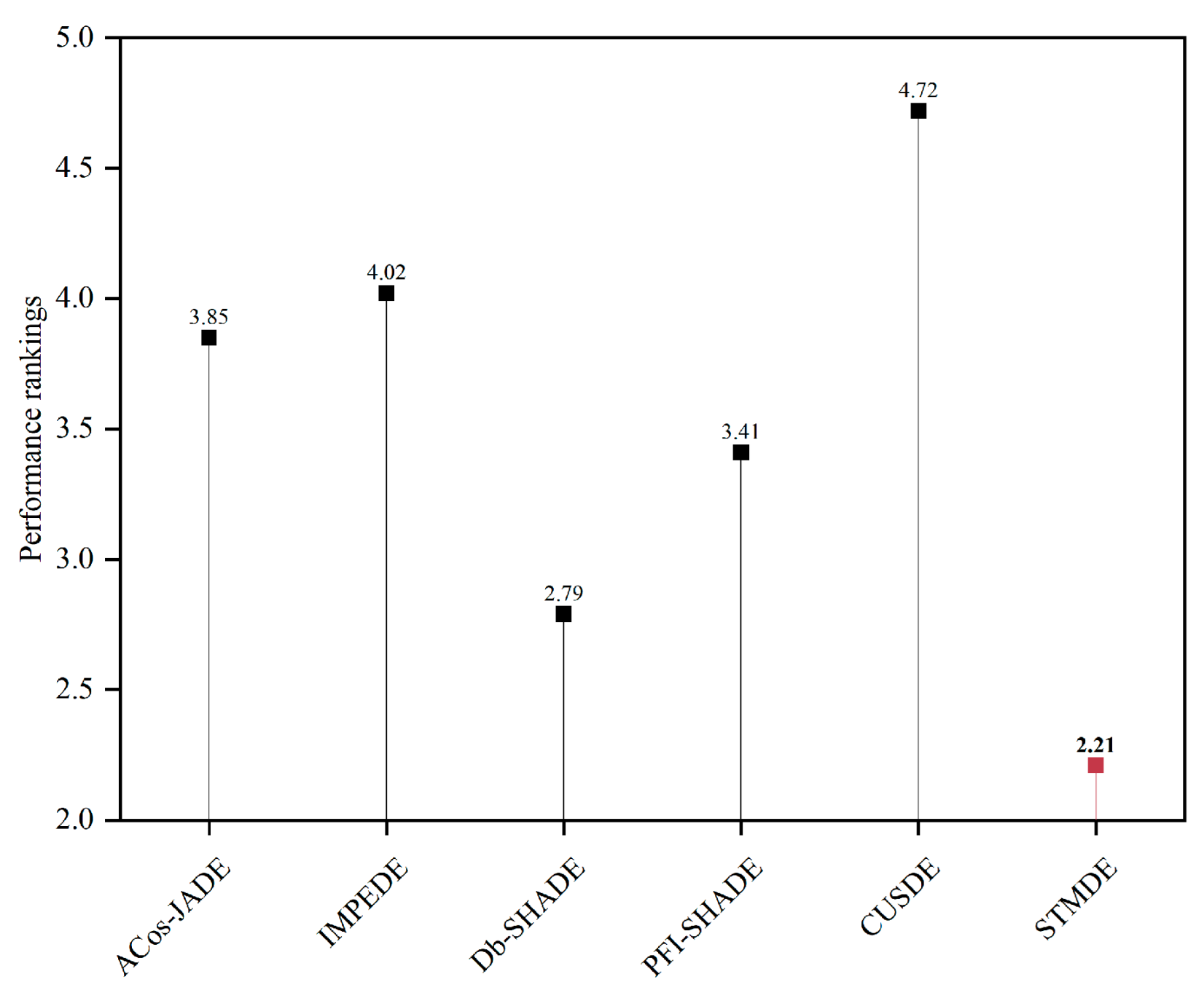
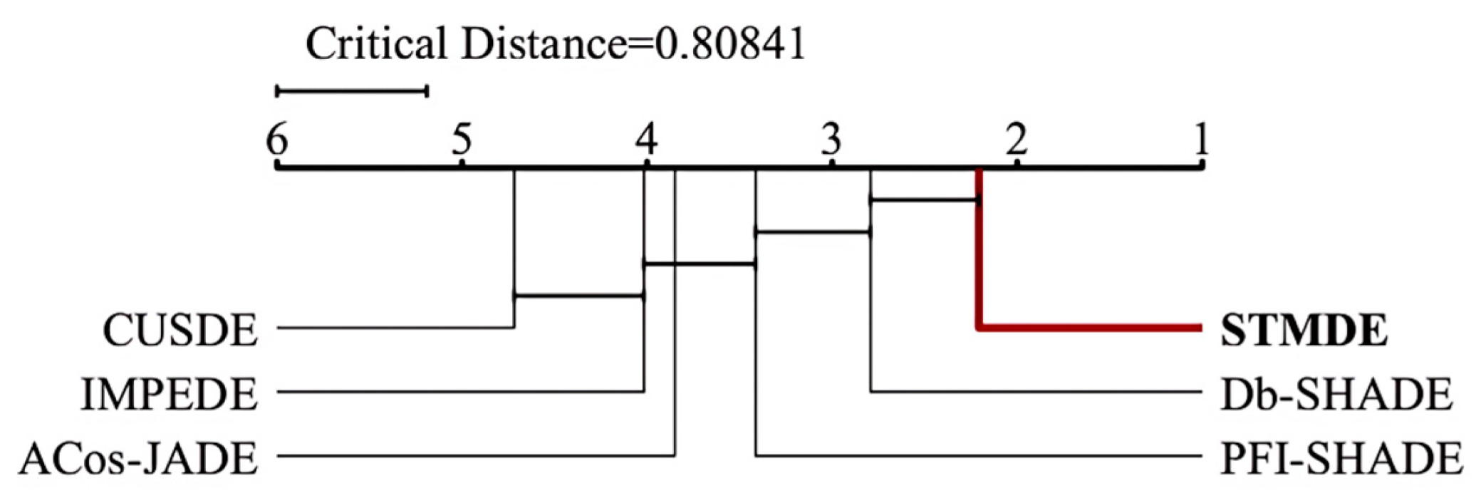
4.2.4. Performance Rankings of STMDE and Compared DE Variants
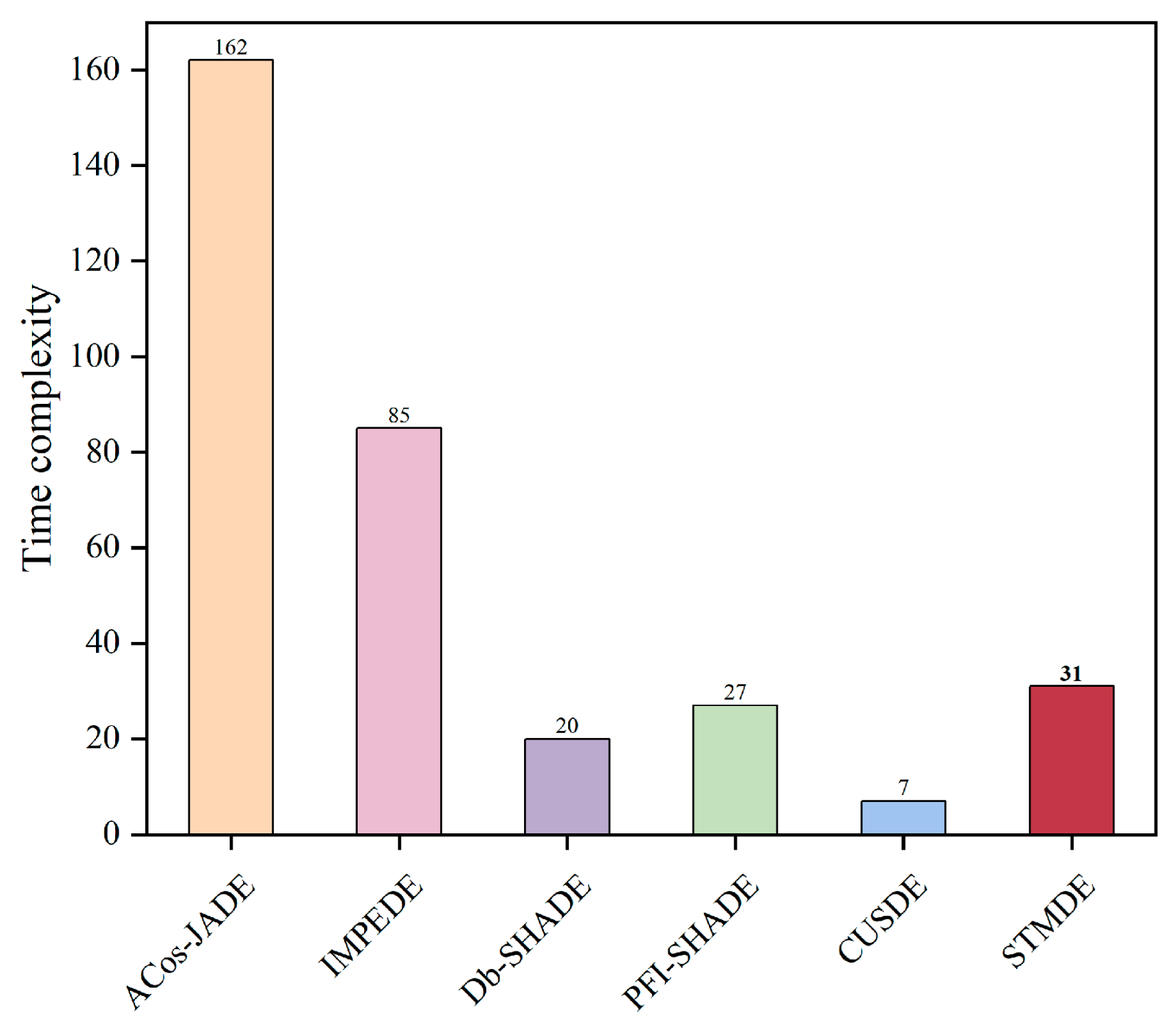
4.2.5. Experimental Time Complexity
4.2.6. Effectiveness of Mechanisms
- (1)
- Variant 1: deactivate the CPSR scheme and other processes are the same as the STMDE;
- (2)
- Variant 2: deactivate the GPSR scheme and other processes are the same as the STMDE;
- (3)
- Variant 3: deactivate the GBS scheme and other processes are the same as the STMDE.
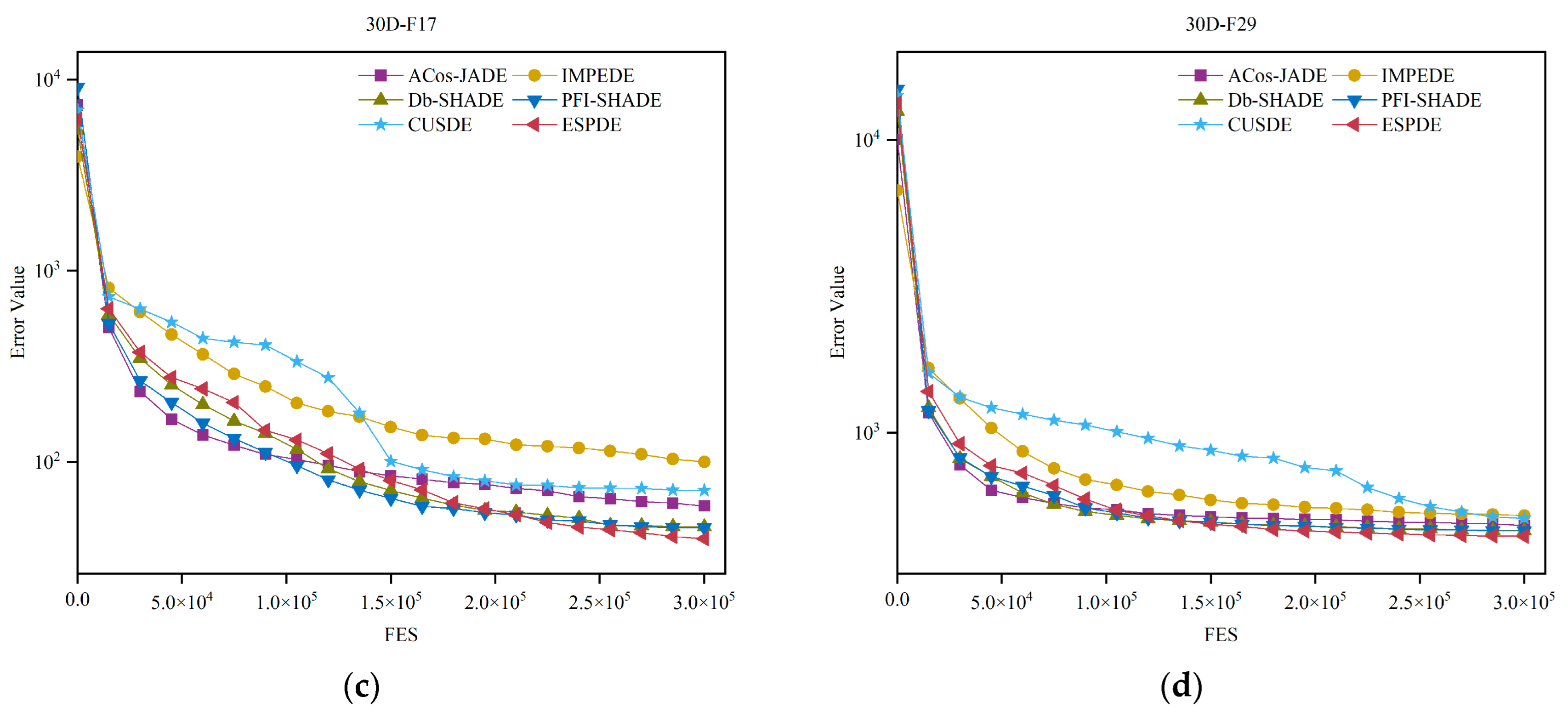
4.2.7. Convergence Graphics
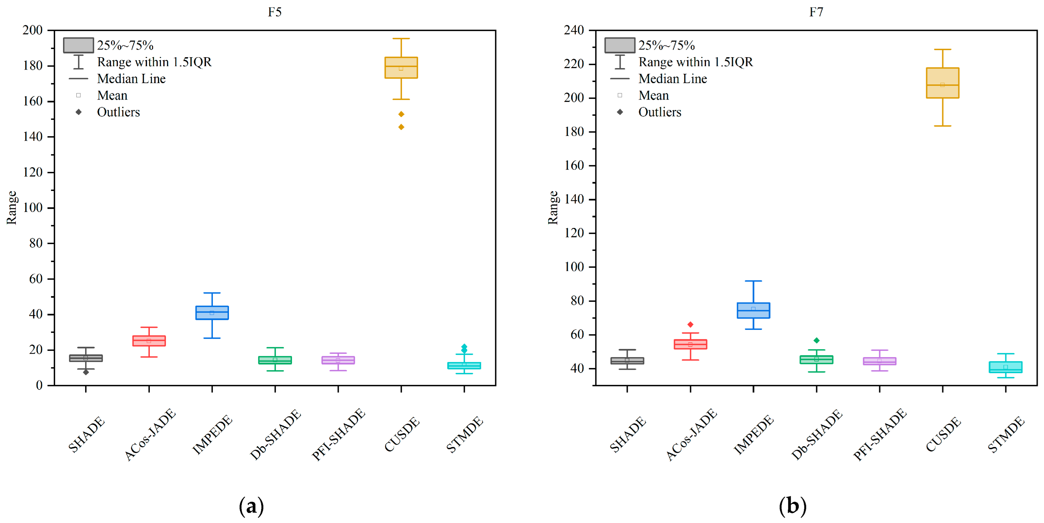
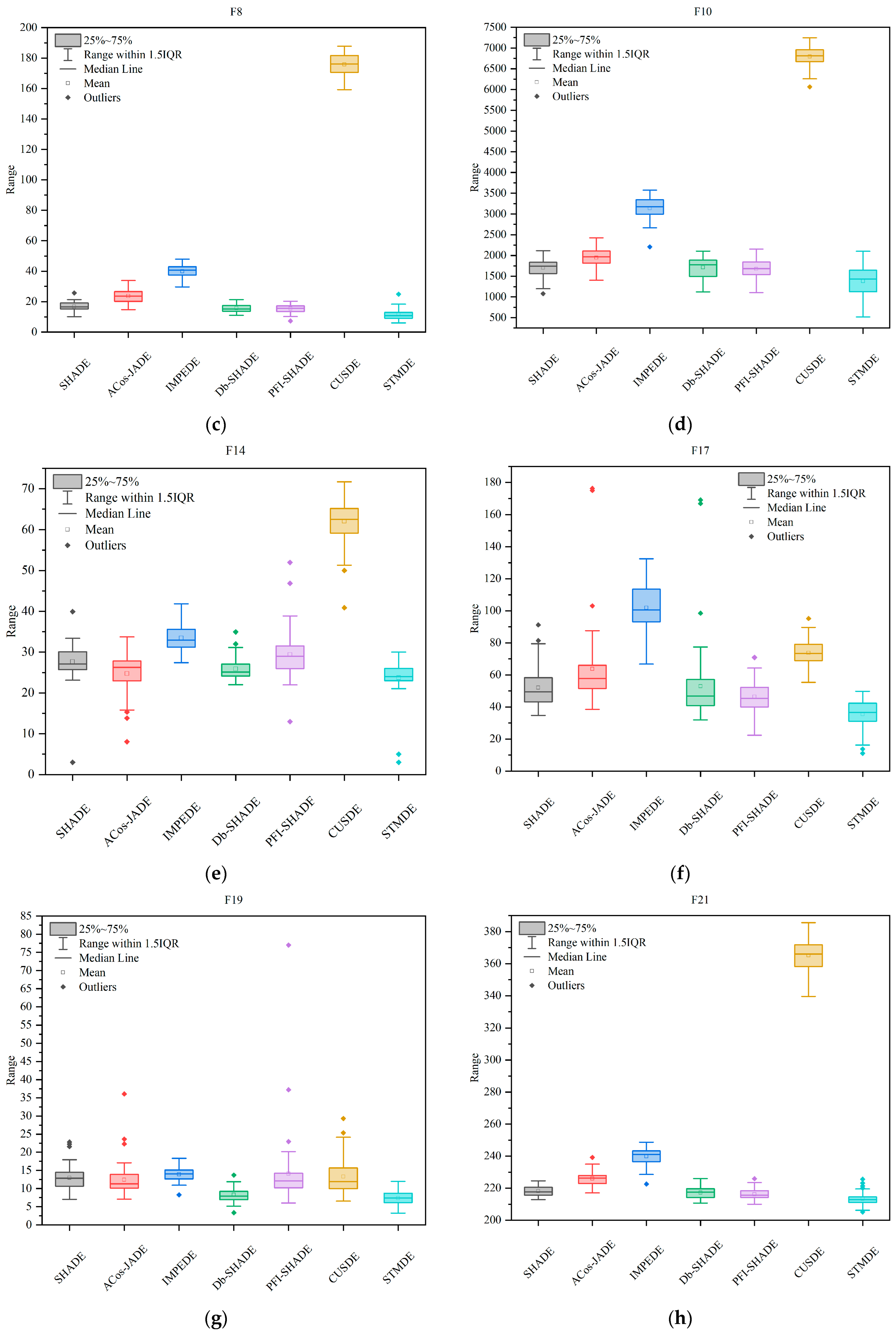
4.2.8. Box Plots of Error
4.2.9. The Analysis of Parameter Sensitivity
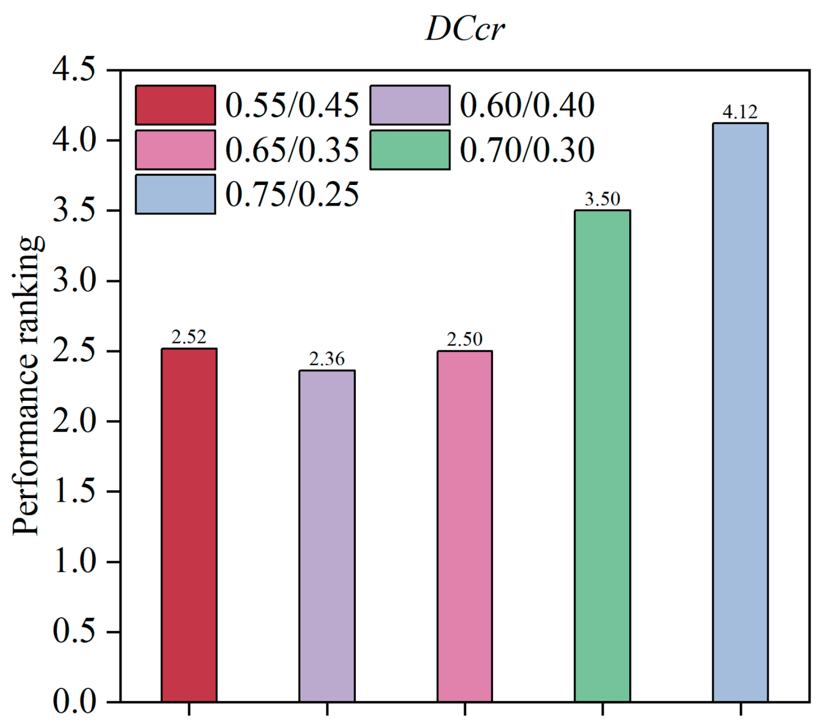
- (1)
- To investigate the parameter sensitivity of DCcr, the GBS scheme is deactivated. From Figure 6, it can be observed that a similar performance is achieved when the DCcr is 0.55/0.45, 0.60/0.40 and 0.65/0.35 (Note: the DCcr is 0.55/0.45 when the STR is larger than 0.5. And the setting is 0.45/0.55 when the STR is smaller than 0.5). Therefore, it is feasible to select one of the settings from 0.55/0.45, 0.60/0.40 and 0.65/0.35. It is worth mentioning that 0.55/0.45 is adopted in the STMDE.
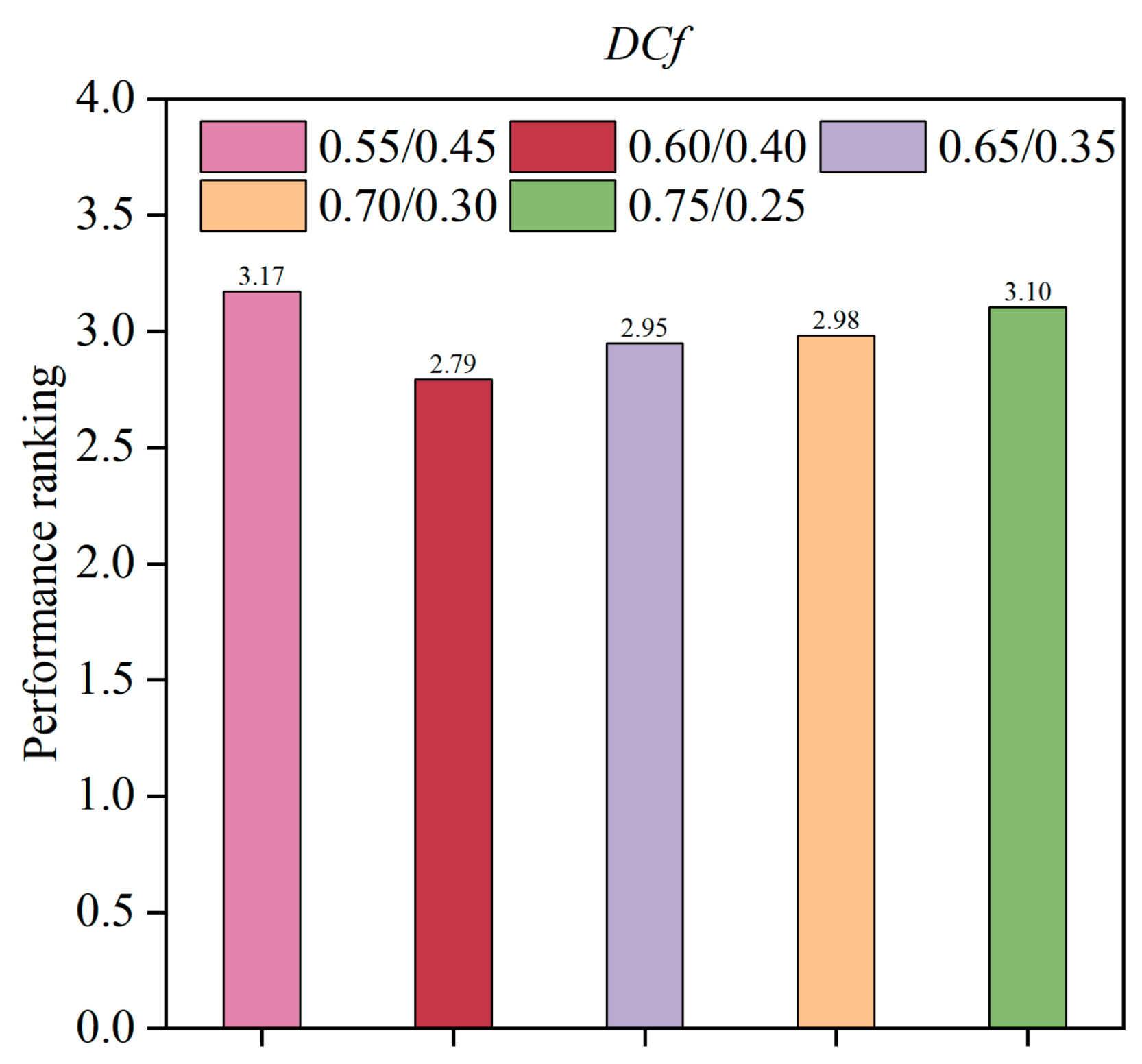
- (2)
- Similarly, the parameter sensitivity of DCf is investigated via deactivating the GBS scheme. From Figure 7, similar performances can be observed when the DCf is 0.60/0.40, 0.65/0.35 and 0.70/0.30 (Note: the DCf is 0.60/0.40 when the STR is larger than 0.5. And the setting is 0.40/0.60 when the STR is smaller than 0.5). Therefore, it is reasonable to select one of the settings from 0.60/0.40, 0.65/0.35 and 0.70/0.30. It is worth mentioning that 0.60/0.40 is adopted in the STMDE.
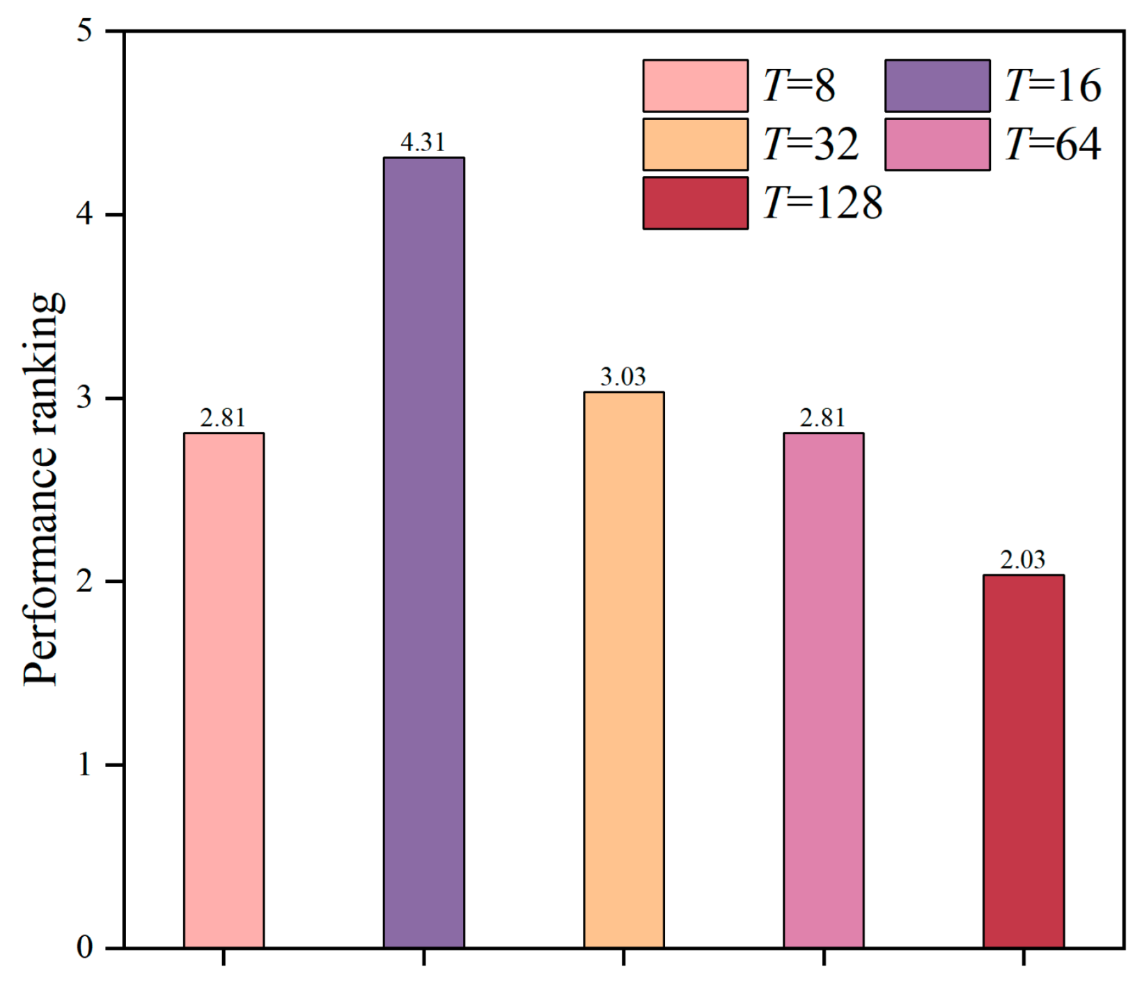
- (3)
- To investigate the parameter sensitivity of threshold T, the PASR is deactivated. From Figure 8, it can be observed that the best performance is obtained when the threshold T is 128.
- (4)
- Apart from the threshold T, the parameter gp of the GBS scheme is also discussed in this subsection. It can be observed from Figure 9 that the performance rankings are similar when the values of gp are 0.5 and 0.7. In this paper, we set the gp as 0.7 when implementing the STMDE.
4.3. Performance Comparison on the Real-World Optimization Problem
5. Conclusions
Author Contributions
Funding
Data Availability Statement
Conflicts of Interest
References
- Storn, R.; Price, K. Differential evolution—A simple and efficient heuristic for global optimization over continuous spaces. J. Glob. Optm. 1997, 11, 341–359. [Google Scholar] [CrossRef]
- Zhang, J.; Sanderson, A.C. JADE: Adaptive differential evolution with optional external archive. IEEE Trans. Evol. Comput. 2009, 13, 945–958. [Google Scholar] [CrossRef]
- Tanabe, R.; Fukunaga, A. Success-history based parameter adaptation for differential evolution. In Proceedings of the 2013 IEEE Congress on Evolutionary Computation, Cancun, Mexico, 20–23 June 2013; pp. 71–78. [Google Scholar]
- Meng, Z.; Yang, C. Hip-DE: Historical population based mutation strategy in differential evolution with parameter adaptive mechanism. Inf. Sci. 2021, 562, 44–77. [Google Scholar] [CrossRef]
- Li, S.; Gu, Q.; Gong, W.; Ning, B. An enhanced adaptive differential evolution algorithm for parameter extraction of photovoltaic models. Energy Convers. Manag. 2020, 205, 112443. [Google Scholar] [CrossRef]
- Tong, L.; Dong, M.; Jing, C. An improved multi-population ensemble differential evolution. Neurocomputing 2018, 290, 130–147. [Google Scholar] [CrossRef]
- Gupta, S.; Su, R. An efficient differential evolution with fitness-based dynamic mutation strategy and control parameters. Knowl.-Based Syst. 2022, 251, 109280. [Google Scholar] [CrossRef]
- Yu, W.J.; Shen, M.; Chen, W.N.; Zhan, Z.H.; Gong, Y.J.; Lin, Y.; Zhang, J. Differential evolution with two-level parameter adaptation. IEEE Trans. Cybern. 2013, 44, 1080–1099. [Google Scholar] [CrossRef]
- Tang, L.; Dong, Y.; Liu, J. Differential evolution with an individual-dependent mechanism. IEEE Trans. Evol. Comput. 2014, 19, 560–574. [Google Scholar] [CrossRef]
- Viktorin, A.; Senkerik, R.; Pluhacek, M.; Kadavy, T.; Zamuda, A. Distance based parameter adaptation for success-history based differential evolution. Swarm Evol. Comput. 2019, 50, 100462. [Google Scholar] [CrossRef]
- Cao, Z.; Wang, Z.; Fu, Y.; Jia, H.; Tian, F. An adaptive differential evolution framework based on population feature information. Inf. Sci. 2022, 608, 1416–1440. [Google Scholar] [CrossRef]
- Stanovov, V.; Akhmedova, S.; Semenkin, E. The automatic design of parameter adaptation techniques for differential evolution with genetic programming. Knowl.-Based Syst. 2022, 239, 108070. [Google Scholar] [CrossRef]
- Gao, S.; Yu, Y.; Wang, Y.; Wang, J.; Cheng, J.; Zhou, M. Chaotic local search-based differential evolution algorithms for optimization. IEEE Trans. Syst. Man Cybern. Syst. 2019, 51, 3954–3967. [Google Scholar] [CrossRef]
- Zhao, F.; Zhao, L.; Wang, L.; Song, H. An ensemble discrete differential evolution for the distributed blocking flowshop scheduling with minimizing makespan criterion. Expert Syst. Appl. 2020, 160, 113678. [Google Scholar] [CrossRef]
- Zhang, G.; Xing, K.; Cao, F. Discrete differential evolution algorithm for distributed blocking flowshop scheduling with makespan criterion. Eng. Appl. Artif. Intel. 2018, 76, 96–107. [Google Scholar] [CrossRef]
- Tian, M.; Gao, X.; Dai, C. Differential evolution with improved individual-based parameter setting and selection strategy. Appl. Soft Comput. 2017, 56, 286–297. [Google Scholar] [CrossRef]
- Guo, J.; Li, Z.; Yang, S. Accelerating differential evolution based on a subset-to-subset survivor selection operator. Soft Comput. 2019, 23, 4113–4130. [Google Scholar] [CrossRef]
- Zhang, S.X.; Chan, W.S.; Peng, Z.K.; Zheng, S.Y.; Tang, K.S. Selective-candidate framework with similarity selection rule for evolutionary optimization. Swarm Evol. Comput. 2020, 56, 100696. [Google Scholar] [CrossRef]
- Zeng, Z.; Zhang, M.; Chen, T.; Hong, Z. A new selection operator for differential evolution algorithm. Knowl.-Based Syst. 2021, 226, 107150. [Google Scholar] [CrossRef]
- Chen, F.; Shi, J.; Ma, Y.; Lei, Y.; Gong, M. Differential evolution algorithm with learning selection strategy for SAR image change detection. In Proceedings of the 2017 IEEE Congress on Evolutionary Computation, Donostia, Spain, 5–8 June 2017; pp. 450–457. [Google Scholar]
- Liang, J.J.; Qu, B.Y.; Suganthan, P.N. Problem Definitions and Evaluation Criteria for the CEC 2017 Special Session and Competition on Single Objective Bound Constrained Real-Parameter Numerical Optimization; Technical Report; Nanyang Technological University Singapore: Singapore, 2016; pp. 1–34. [Google Scholar]
- Das, S.; Suganthan, P.N. Problem Definitions and Evaluation Criteria for CEC 2011 Competition on Testing Evolutionary Algorithms on Real World Optimization Problems; Jadavpur University: Kolkata, India; Nanyang Technological University: Singapore, 2010; pp. 341–359. [Google Scholar]
- Liu, Z.Z.; Wang, Y.; Yang, S.; Tang, K. An adaptive framework to tune the coordinate systems in nature-inspired optimization algorithms. IEEE Trans. Cybern. 2018, 49, 1403–1416. [Google Scholar] [CrossRef]
- Zou, L.; Pan, Z.; Gao, Z.; Gao, J. Improving the search accuracy of differential evolution by using the number of consecutive unsuccessful updates. Knowl.-Based Syst. 2022, 250, 109005. [Google Scholar] [CrossRef]
- Sheskin, D.J. Handbook of Parametric and Nonparametric Statistical Procedures; Chapman and Hall/CRC: New York, NY, USA, 2003. [Google Scholar]
- Demšar, J. Statistical comparisons of classifiers over multiple data sets. J. Mach. Learn. Res. 2006, 7, 1–30. [Google Scholar]


| 30-D | 50-D | 100-D | |||||||||||||
|---|---|---|---|---|---|---|---|---|---|---|---|---|---|---|---|
| SHADE | STMDE | SHADE | STMDE | SHADE | STMDE | ||||||||||
| mean | std | sig | mean | std | mean | std | sig | mean | std | mean | std | sig | mean | std | |
| F1 | 1.00 × 10⁻¹⁴ | 6.54 × 10⁻¹⁵ | = | 8.36 × 10⁻¹⁵ | 7.06 × 10⁻¹⁵ | 3.82 × 10⁻¹⁴ | 1.38 × 10⁻¹⁴ | = | 3.76 × 10⁻¹⁴ | 1.33 × 10⁻¹⁴ | 8.13 × 10⁻¹¹ | 1.82 × 10⁻¹⁰ | + | 4.94 × 10⁻¹¹ | 1.59 × 10⁻¹⁰ |
| F3 | 6.80 × 10⁻¹⁴ | 2.28 × 10⁻¹⁴ | = | 6.58 × 10⁻¹⁴ | 2.38 × 10⁻¹⁴ | 5.98 × 10⁻¹² | 1.70 × 10⁻¹¹ | + | 4.24 × 10⁻¹³ | 2.50 × 10⁻¹³ | 7.96 × 10⁻⁸ | 1.96 × 10⁻⁷ | − | 2.62 × 10⁻³ | 1.14 × 10⁻² |
| F4 | 4.88 × 101 | 2.27 × 101 | = | 5.66 × 101 | 1.16 × 101 | 5.25 × 101 | 4.58 × 101 | = | 4.63 × 101 | 4.26 × 101 | 1.24 × 10² | 6.22 × 101 | = | 1.27 × 10² | 6.95 × 101 |
| F5 | 1.54 × 101 | 2.89 × 100 | + | 1.17 × 101 | 3.48 × 100 | 3.84 × 101 | 5.82 × 100 | + | 2.83 × 101 | 8.71 × 100 | 1.00 × 10² | 1.21 × 101 | = | 9.98 × 101 | 1.52 × 101 |
| F6 | 2.44 × 10⁻⁵ | 8.52 × 10⁻⁵ | + | 4.95 × 10⁻⁶ | 1.22 × 10⁻⁵ | 8.37 × 10⁻⁴ | 1.20 × 10⁻³ | = | 6.67 × 10⁻⁴ | 6.68 × 10⁻⁴ | 8.07 × 10⁻² | 5.36 × 10⁻² | + | 2.77 × 10⁻² | 2.29 × 10⁻² |
| F7 | 4.47 × 101 | 2.63 × 100 | + | 4.08 × 101 | 3.88 × 100 | 8.28 × 101 | 5.07 × 100 | + | 7.50 × 101 | 7.02 × 100 | 2.08 × 10² | 1.48 × 101 | + | 1.94 × 10² | 1.79 × 101 |
| F8 | 1.68 × 101 | 3.06 × 100 | + | 1.13 × 101 | 3.33 × 100 | 3.90 × 101 | 5.91 × 100 | + | 2.92 × 101 | 1.12 × 101 | 9.99 × 101 | 1.39 × 101 | = | 9.63 × 101 | 1.76 × 101 |
| F9 | 2.30 × 10⁻² | 6.98 × 10⁻² | = | 1.23 × 10⁻² | 3.11 × 10⁻² | 1.36 × 100 | 1.07 × 100 | + | 4.82 × 10⁻¹ | 4.95 × 10⁻¹ | 2.74 × 101 | 1.15 × 101 | + | 1.46 × 101 | 7.64 × 100 |
| F10 | 1.70 × 10³ | 2.11 × 10² | + | 1.38 × 10³ | 3.65 × 10² | 3.44 × 10³ | 2.92 × 10² | + | 2.73 × 10³ | 4.26 × 10² | 9.18 × 10³ | 5.39 × 10² | + | 8.27 × 10³ | 9.30 × 10² |
| F11 | 3.46 × 101 | 2.64 × 101 | + | 2.27 × 101 | 2.31 × 101 | 1.25 × 10² | 2.93 × 101 | + | 1.08 × 10² | 2.65 × 101 | 1.13 × 10³ | 1.96 × 10² | + | 8.81 × 10² | 2.42 × 10² |
| F12 | 1.26 × 10³ | 3.11 × 10² | = | 1.10 × 10³ | 4.10 × 10² | 7.36 × 10³ | 7.49 × 10³ | = | 6.13 × 10³ | 4.55 × 10³ | 1.92 × 10⁴ | 1.24 × 10⁴ | − | 2.37 × 10⁴ | 9.06 × 10³ |
| F13 | 4.15 × 101 | 2.76 × 101 | + | 2.39 × 101 | 9.97 × 100 | 2.27 × 10² | 1.54 × 10² | + | 1.38 × 10² | 8.51 × 101 | 1.93 × 10³ | 3.84 × 10³ | = | 3.31 × 10² | 1.69 × 10² |
| F14 | 2.77 × 101 | 4.70 × 100 | + | 2.37 × 101 | 4.49 × 100 | 1.88 × 10² | 3.81 × 101 | + | 8.87 × 101 | 3.36 × 101 | 5.84 × 10² | 1.83 × 10² | = | 5.50 × 10² | 1.17 × 10² |
| F15 | 1.81 × 101 | 1.03 × 101 | + | 9.05 × 100 | 4.56 × 100 | 2.21 × 10² | 1.03 × 10² | + | 1.43 × 10² | 7.94 × 101 | 3.19 × 10² | 8.06 × 101 | − | 4.49 × 10² | 2.28 × 10² |
| F16 | 3.28 × 10² | 1.20 × 10² | + | 2.52 × 10² | 1.38 × 10² | 7.67 × 10² | 1.97 × 10² | + | 6.31 × 10² | 2.22 × 10² | 2.41 × 10³ | 3.32 × 10² | = | 2.34 × 10³ | 4.31 × 10² |
| F17 | 5.20 × 101 | 1.26 × 101 | + | 3.55 × 101 | 9.66 × 100 | 5.87 × 10² | 1.25 × 10² | + | 4.42 × 10² | 1.35 × 10² | 1.82 × 10³ | 2.99 × 10² | + | 1.65 × 10³ | 3.72 × 10² |
| F18 | 4.11 × 101 | 3.52 × 101 | + | 2.80 × 101 | 8.17 × 100 | 1.78 × 10² | 1.22 × 10² | = | 1.74 × 10² | 1.10 × 10² | 1.39 × 10³ | 9.44 × 10² | = | 2.08 × 10³ | 2.04 × 10³ |
| F19 | 1.29 × 101 | 3.52 × 100 | + | 7.39 × 100 | 2.12 × 100 | 1.30 × 10² | 4.53 × 101 | + | 9.69 × 101 | 3.87 × 101 | 3.18 × 10² | 4.89 × 10² | = | 2.41 × 10² | 5.01 × 101 |
| F20 | 9.09 × 101 | 5.54 × 101 | + | 5.64 × 101 | 5.42 × 101 | 3.95 × 10² | 9.93 × 101 | + | 3.16 × 10² | 1.57 × 10² | 1.70 × 10³ | 2.29 × 10² | + | 1.57 × 10³ | 3.65 × 10² |
| F21 | 2.18 × 10² | 3.12 × 100 | + | 2.13 × 10² | 4.01 × 100 | 2.36 × 10² | 5.09 × 100 | + | 2.31 × 10² | 8.33 × 100 | 3.32 × 10² | 1.43 × 101 | + | 3.25 × 10² | 1.51 × 101 |
| F22 | 1.00 × 10² | 3.44 × 10⁻¹ | = | 1.00 × 10² | 6.39 × 10⁻¹⁴ | 1.85 × 10³ | 2.01 × 10³ | = | 2.44 × 10³ | 1.52 × 10³ | 1.05 × 10⁴ | 5.00 × 10² | + | 9.78 × 10³ | 1.27 × 10³ |
| F23 | 3.64 × 10² | 4.52 × 100 | + | 3.60 × 10² | 4.91 × 100 | 4.61 × 10² | 6.82 × 100 | + | 4.57 × 10² | 1.32 × 101 | 6.12 × 10² | 1.44 × 101 | + | 5.98 × 10² | 1.95 × 101 |
| F24 | 4.35 × 10² | 3.76 × 100 | = | 4.35 × 10² | 6.18 × 100 | 5.31 × 10² | 5.88 × 100 | = | 5.33 × 10² | 9.59 × 100 | 9.92 × 10² | 2.13 × 101 | = | 1.00 × 10³ | 2.20 × 101 |
| F25 | 3.87 × 10² | 2.04 × 10⁻¹ | + | 3.87 × 10² | 5.10 × 10⁻² | 5.38 × 10² | 3.22 × 101 | = | 5.25 × 10² | 3.43 × 101 | 7.43 × 10² | 5.48 × 101 | = | 7.40 × 10² | 4.27 × 101 |
| F26 | 1.11 × 10³ | 5.44 × 101 | + | 1.08 × 10³ | 8.15 × 101 | 1.45 × 10³ | 9.00 × 101 | = | 1.44 × 10³ | 1.10 × 10² | 4.23 × 10³ | 2.13 × 10² | = | 4.28 × 10³ | 2.47 × 10² |
| F27 | 5.05 × 10² | 6.01 × 100 | = | 5.05 × 10² | 5.52 × 100 | 5.43 × 10² | 2.59 × 101 | + | 5.33 × 10² | 1.31 × 101 | 6.70 × 10² | 3.48 × 101 | + | 6.47 × 10² | 2.51 × 101 |
| F28 | 3.43 × 10² | 5.83 × 101 | = | 3.41 × 10² | 5.41 × 101 | 4.97 × 10² | 1.68 × 101 | + | 4.80 × 10² | 2.40 × 101 | 5.34 × 10² | 3.77 × 101 | = | 5.32 × 10² | 3.00 × 101 |
| F29 | 4.63 × 10² | 1.10 × 101 | + | 4.47 × 10² | 1.90 × 101 | 4.99 × 10² | 8.17 × 101 | + | 4.04 × 10² | 7.97 × 101 | 2.13 × 10³ | 2.94 × 10² | + | 1.91 × 10³ | 2.94 × 10² |
| F30 | 2.07 × 10³ | 9.51 × 101 | = | 2.04 × 10³ | 7.55 × 101 | 6.53 × 10⁵ | 6.51 × 10⁴ | = | 6.68 × 10⁵ | 8.37 × 10⁴ | 2.75 × 10³ | 7.83 × 10² | + | 2.53 × 10³ | 1.86 × 10² |
| W/T/L | 19/10/0 | 19/10/0 | 14/12/3 | ||||||||||||
| Variant | Unimodal Functions | Simple Multi-Modal Functions | Hybrid Functions | Composition Functions | Overall |
|---|---|---|---|---|---|
| Variant 1 | 1/1 | 3/0 | 7/0 | 4/0 | 15/1 |
| Variant 2 | 1/1 | 6/0 | 4/0 | 2/0 | 13/1 |
| Variant 3 | 1/1 | 5/0 | 3/0 | 3/0 | 12/1 |
| FES | 5.00 × 10⁴ | 1.00 × 10⁵ | 1.50 × 10⁵ | ||||||||||
|---|---|---|---|---|---|---|---|---|---|---|---|---|---|
| DEs | mean | std | sig | mean | std | sig | mean | std | sig | ||||
| SHADE | 1.36 × 100 | 1.02 × 10⁻¹ | = | 1.24 × 100 | 1.05 × 10⁻¹ | + | 1.24 × 100 | 8.13 × 10⁻² | + | ||||
| ACos-JADE | 1.37 × 100 | 1.07 × 10⁻¹ | = | 1.19 × 100 | 9.03 × 10⁻² | + | 1.14 × 100 | 9.27 × 10⁻² | + | ||||
| IMPEDE | 1.37 × 100 | 5.39 × 10⁻² | = | 1.19 × 100 | 1.00 × 10⁻¹ | + | 1.13 × 100 | 9.57 × 10⁻² | + | ||||
| Db-SHADE | 1.36 × 100 | 1.03 × 10⁻¹ | = | 1.25 × 100 | 1.12 × 10⁻¹ | + | 1.22 × 100 | 1.11 × 10⁻¹ | + | ||||
| PFI-SHADE | 1.40 × 100 | 9.90 × 10⁻² | = | 1.25 × 100 | 1.03 × 10⁻¹ | + | 1.22 × 100 | 9.48 × 10⁻² | + | ||||
| CUSDE | 1.84 × 100 | 9.68 × 10⁻² | + | 1.77 × 100 | 1.15 × 10⁻¹ | + | 1.71 × 100 | 1.08 × 10⁻¹ | + | ||||
| STMDE | 1.37 × 100 | 1.12 × 10⁻¹ | 1.00 × 100 | 2.93 × 10⁻¹ | 8.95 × 101 | 2.47 × 10⁻¹ | |||||||
Disclaimer/Publisher’s Note: The statements, opinions and data contained in all publications are solely those of the individual author(s) and contributor(s) and not of MDPI and/or the editor(s). MDPI and/or the editor(s) disclaim responsibility for any injury to people or property resulting from any ideas, methods, instructions or products referred to in the content. |
© 2024 by the authors. Licensee MDPI, Basel, Switzerland. This article is an open access article distributed under the terms and conditions of the Creative Commons Attribution (CC BY) license (https://creativecommons.org/licenses/by/4.0/).
Share and Cite
Liu, Y.; Zheng, L.; Cai, B. Adaptive Differential Evolution with the Stagnation Termination Mechanism. Mathematics 2024, 12, 3168. https://doi.org/10.3390/math12203168
Liu Y, Zheng L, Cai B. Adaptive Differential Evolution with the Stagnation Termination Mechanism. Mathematics. 2024; 12(20):3168. https://doi.org/10.3390/math12203168
Chicago/Turabian StyleLiu, Yuhong, Liming Zheng, and Bohan Cai. 2024. "Adaptive Differential Evolution with the Stagnation Termination Mechanism" Mathematics 12, no. 20: 3168. https://doi.org/10.3390/math12203168
APA StyleLiu, Y., Zheng, L., & Cai, B. (2024). Adaptive Differential Evolution with the Stagnation Termination Mechanism. Mathematics, 12(20), 3168. https://doi.org/10.3390/math12203168