
Dynamic Malware Mitigation Strategies for IoT Networks: A Mathematical Epidemiology Approach

 ,
,  , ,
, ,  and
and 
Abstract
1. Introduction
- We propose a strategy to mitigate the spread of malware through the installation of security updates on IoT nodes. Node selection is based on two criteria: random selection for updates, and selection based on the degree of IoT nodes.
- Since the propagation parameters of malware are unknown in real-world scenarios, we propose to estimate these parameters by solving the inverse problem with a physics-informed neural network.
- We conducted a numerical study to evaluate our proposal. Moreover, we developed new metrics to assess the effectiveness of the mitigation strategy based on node selection criteria. This assessment suggests that the IoT network-based mitigation approach is more effective.
2. Mitigation Strategies
3. Methods
3.1. Propagation Model for Malware Based on the SIR Classic Model
3.1.1. The Kermack and McKendrick SIR Model
3.1.2. Individual-Based Stochastic SIR Model
- A susceptible device can become infected depending on the infection rate, , of each IoT node, where .
- An infected device can be recovered, depending on the recovery rate, , of each IoT node, where .
- This model considers permanent immunity, preventing the malware from infecting recovered devices.
| Algorithm 1 IB malware spread transition rules pseudocode |
|
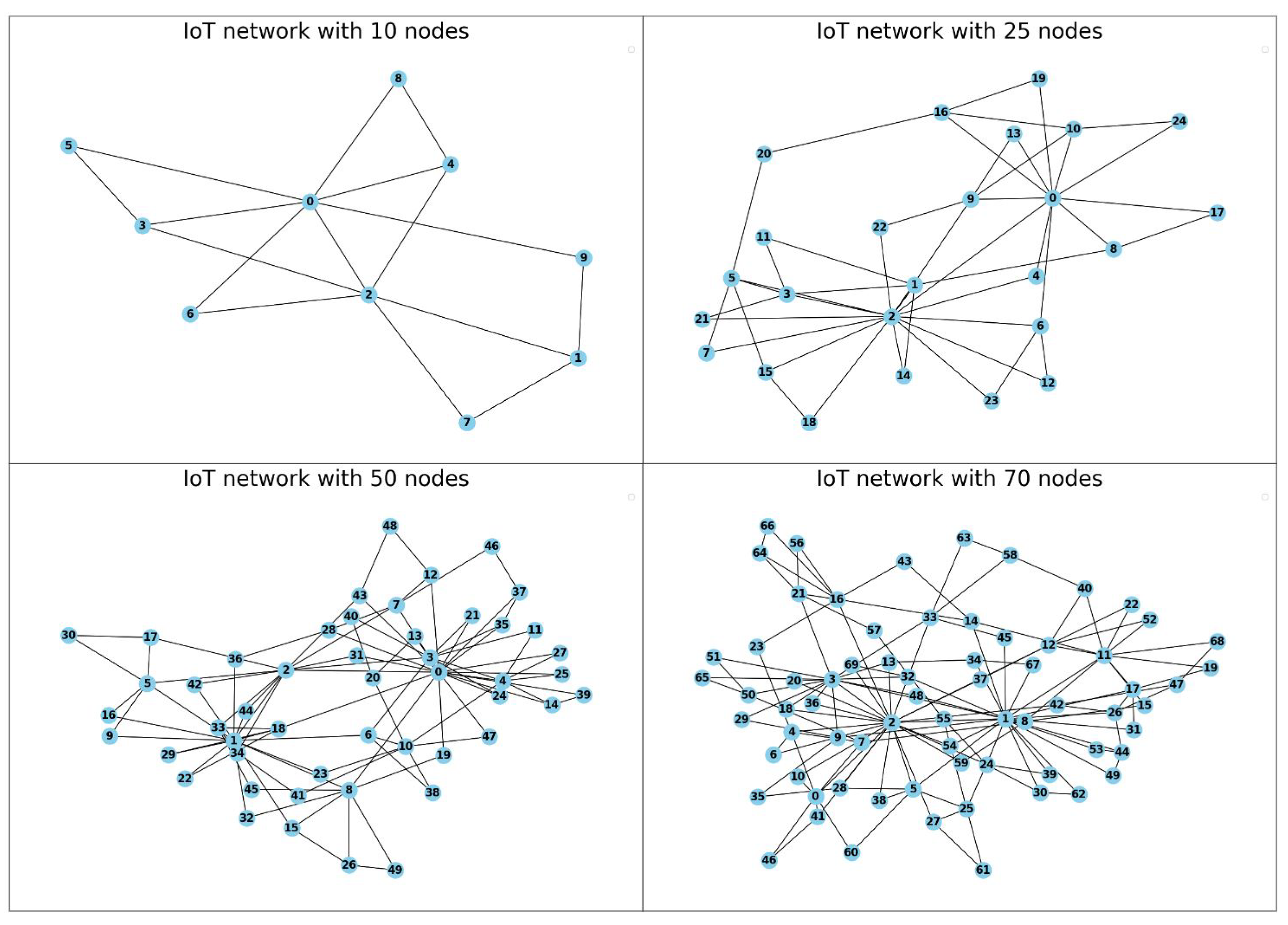
3.2. A Complex Network Approach to IoT Network
- Degree of a node: In an undirected network, a node’s degree is defined as the total number of members connected to it and denoted by . In a simple undirected graph .
- The average degree is defined by the following equation .
3.3. Evaluation Metrics
- Global infection rate: This rate represents the average infection rate from a susceptible device to an infected device. The global infection rate is calculated as the sum of the betas of all devices divided by the total number of devices.where is the infection rate of the device i and N is the number of devices in the IoT network. In this case, we are solving an inverse problem with one PINN for the whole network as the of each device is not fully known at time t.
- Percentage of final susceptibles: The final susceptibles percentage is a metric used to evaluate the proportion of devices that remain uninfected at the end of a simulation. It is calculated by dividing the number of uninfected devices by the total number of devices. A high PFS indicates that mitigation was effective in preventing device infection, while a low PFS indicates that mitigation was less effective or that the malware was highly contagious.
- Average infected speed: The ’Average infected Speed’ metric quantifies the rate at which malware infects devices within the IoT network. It represents the average number of infected devices per time step. It is calculated as follows:The ’Average infected Speed’ metric is a valuable tool for evaluating the performance of a mathematical model that predicts the spread of malware in an IoT network. A high average infection rate indicates that the model predicts rapid malware spread throughout the network.
- Average recovery speed: The metric ’Average recovery speed’ measures the rate at which infected devices recover from malware and are no longer infectious. It is calculated as follows:
3.4. The Inverse Problem for the Parameter Estimation
Solving the Inverse Problem for a SIR Model
4. Results
4.1. Simulation Setup
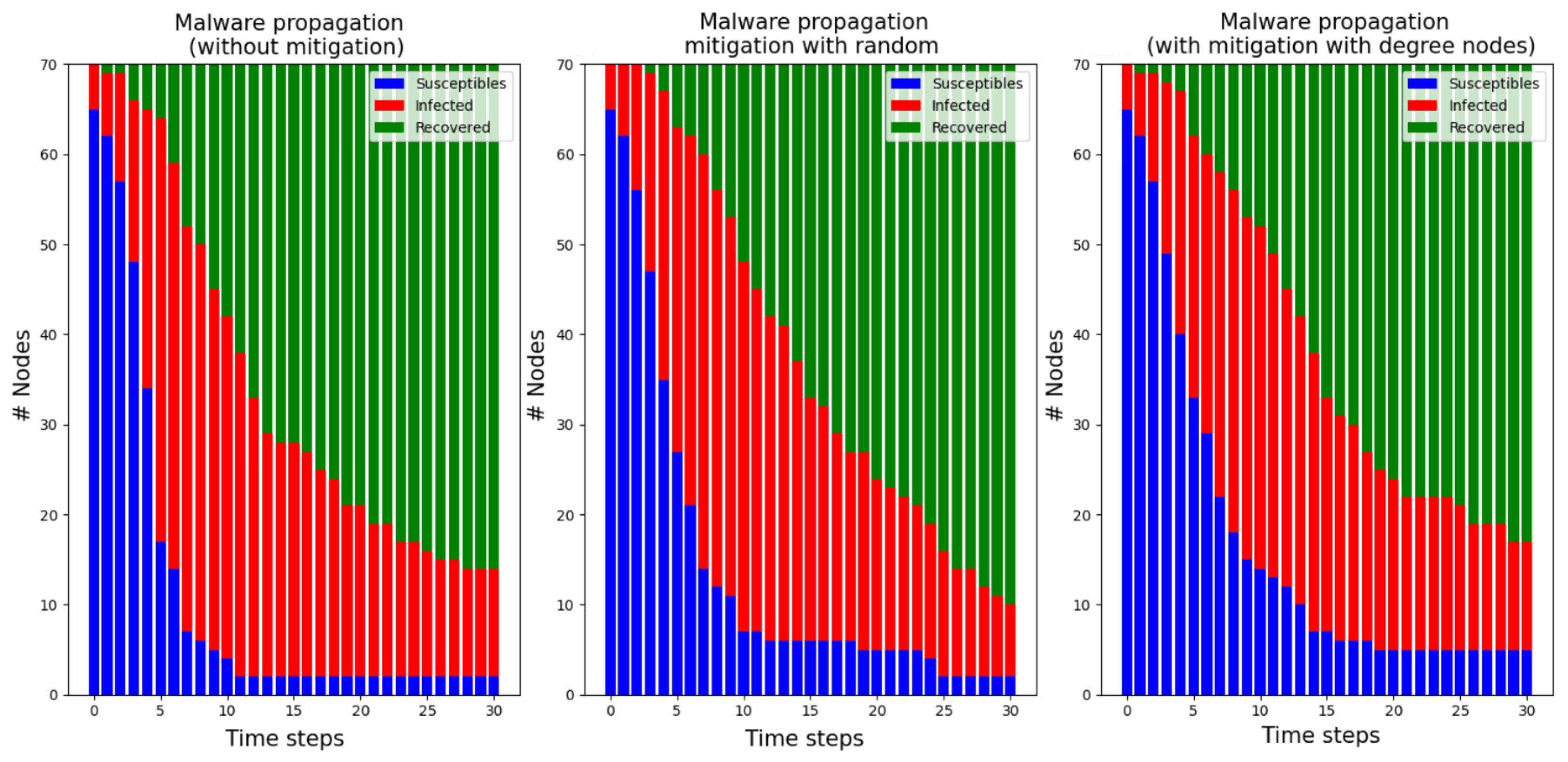
- In Simulation 1, we aim to examine how the number of nodes selected using the random election strategy for patching impacts the spread of malware. The potential choices constitute , and of the entire nodes. Additionally, we assume early detection of malware and implementation of mitigation measures after a brief delay, specifically in time step 4. Finally, we assume the installed security patch to be highly effective, with beta_patched_node .
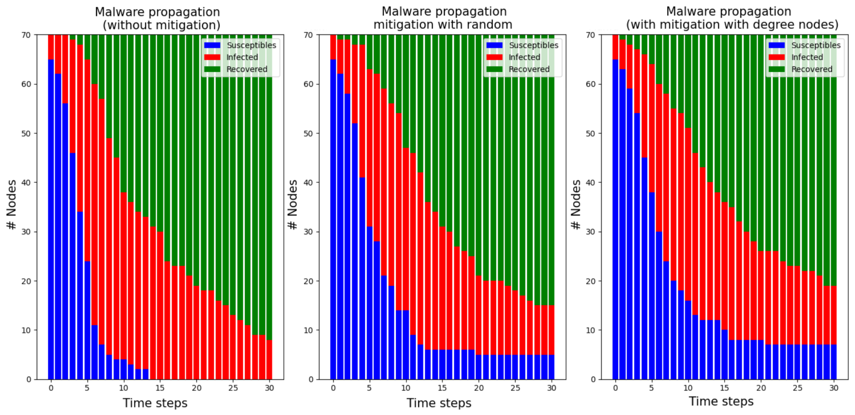
- In Simulation 2, we aim to observe the impact of early detection and subsequent security patching on malware propagation dynamics. By evaluating various early time steps = , we can assess the mitigation measures’ performance with the two-node election strategies. Additionally, for this simulation, we will choose 25% of the nodes using the random strategy. Finally, it is assumed that the installed security patch is highly effective, with beta_patched_node .
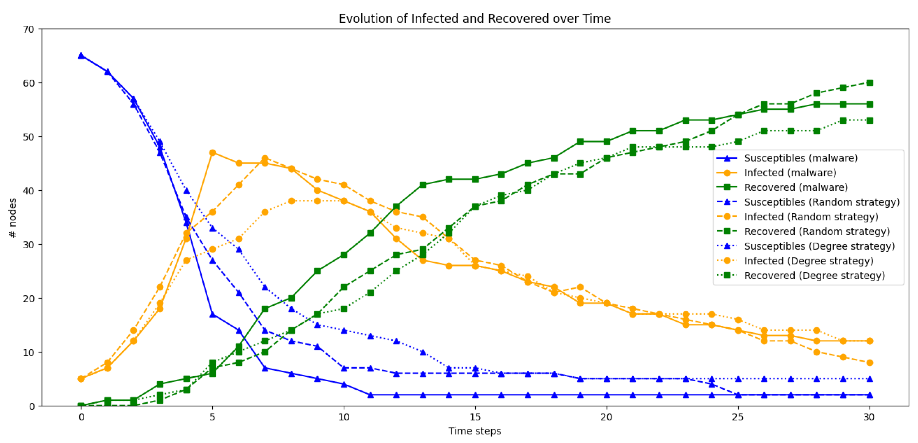
4.2. Simulation Results
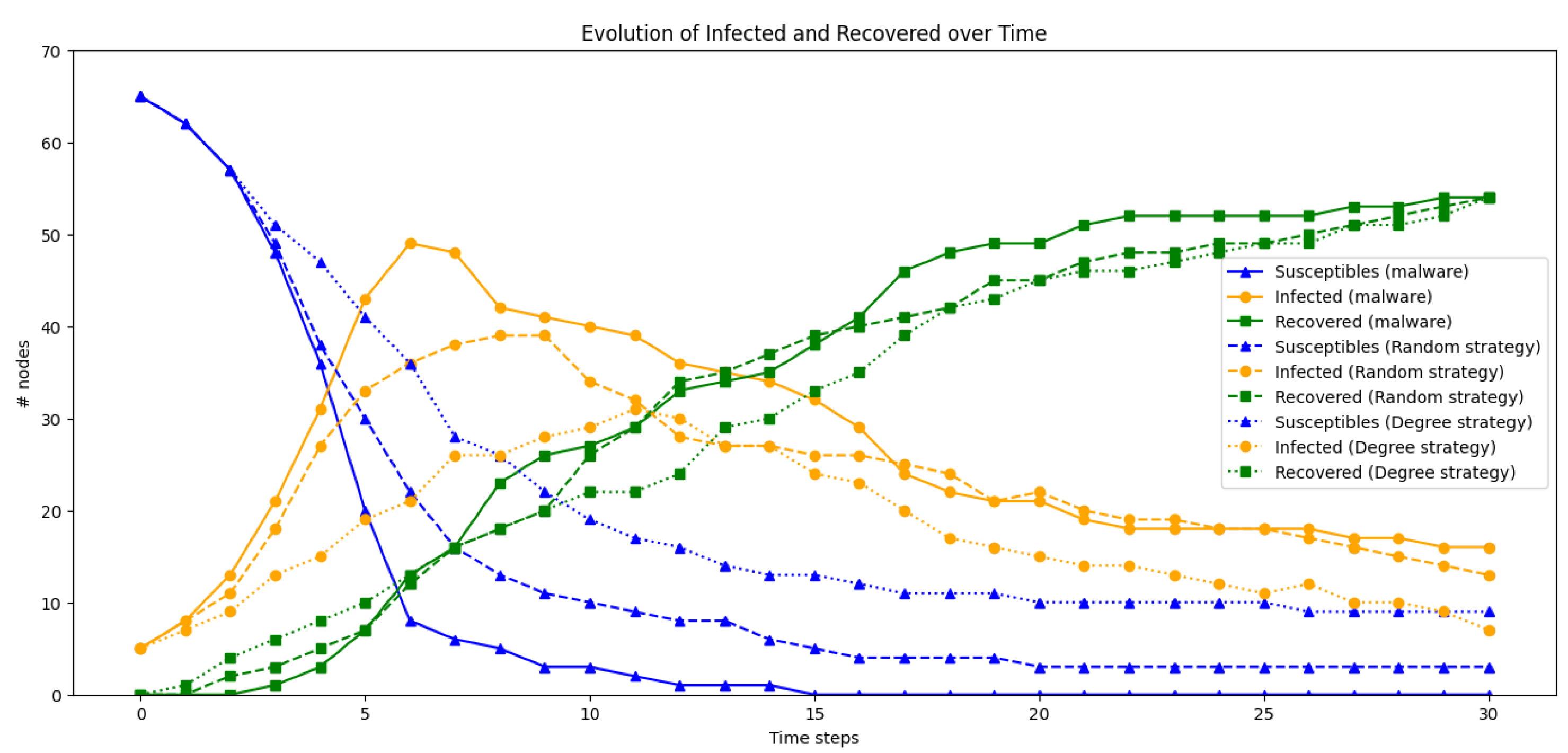
4.2.1. Simulation 1.1 with Nodes, Patching , Early Patching Time Step
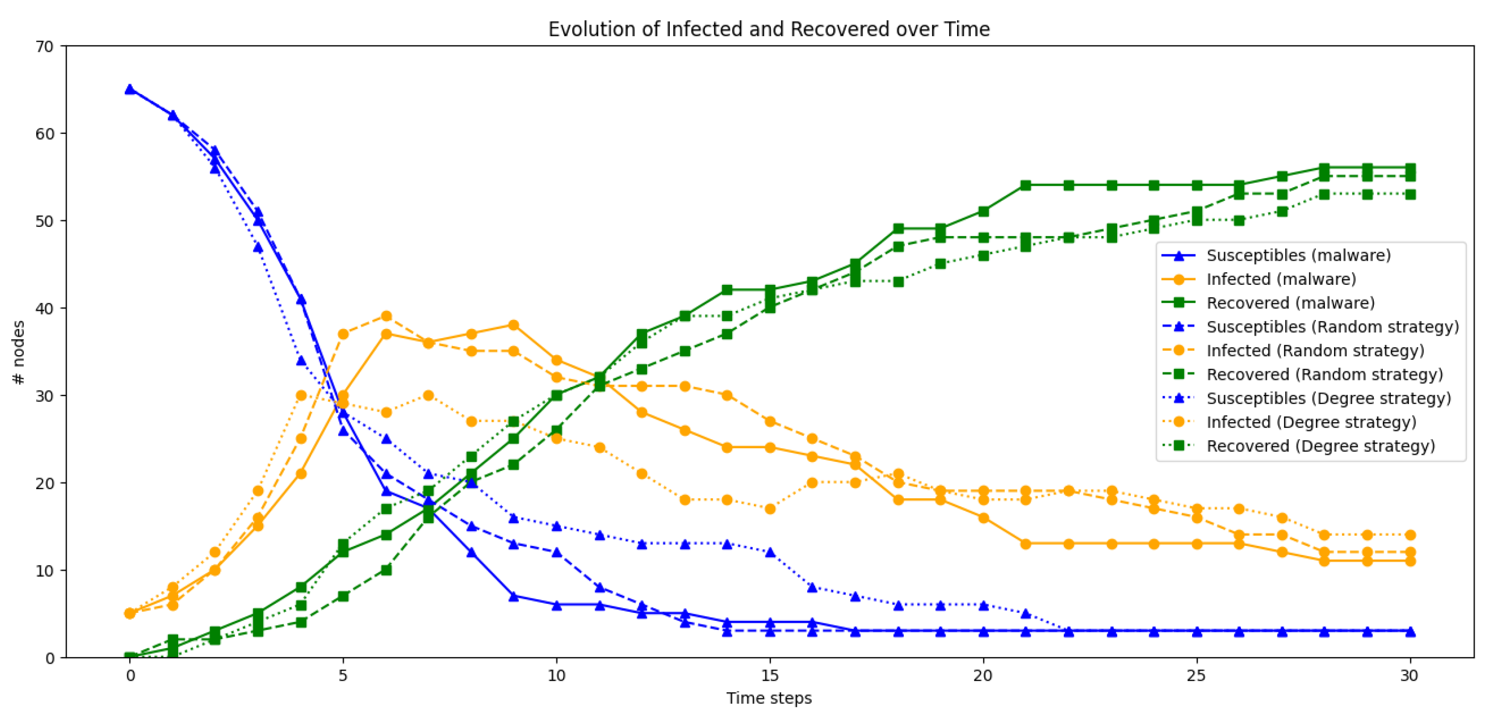
4.2.2. Simulation 1.2 with Nodes, Patching , Early Patching Time Step
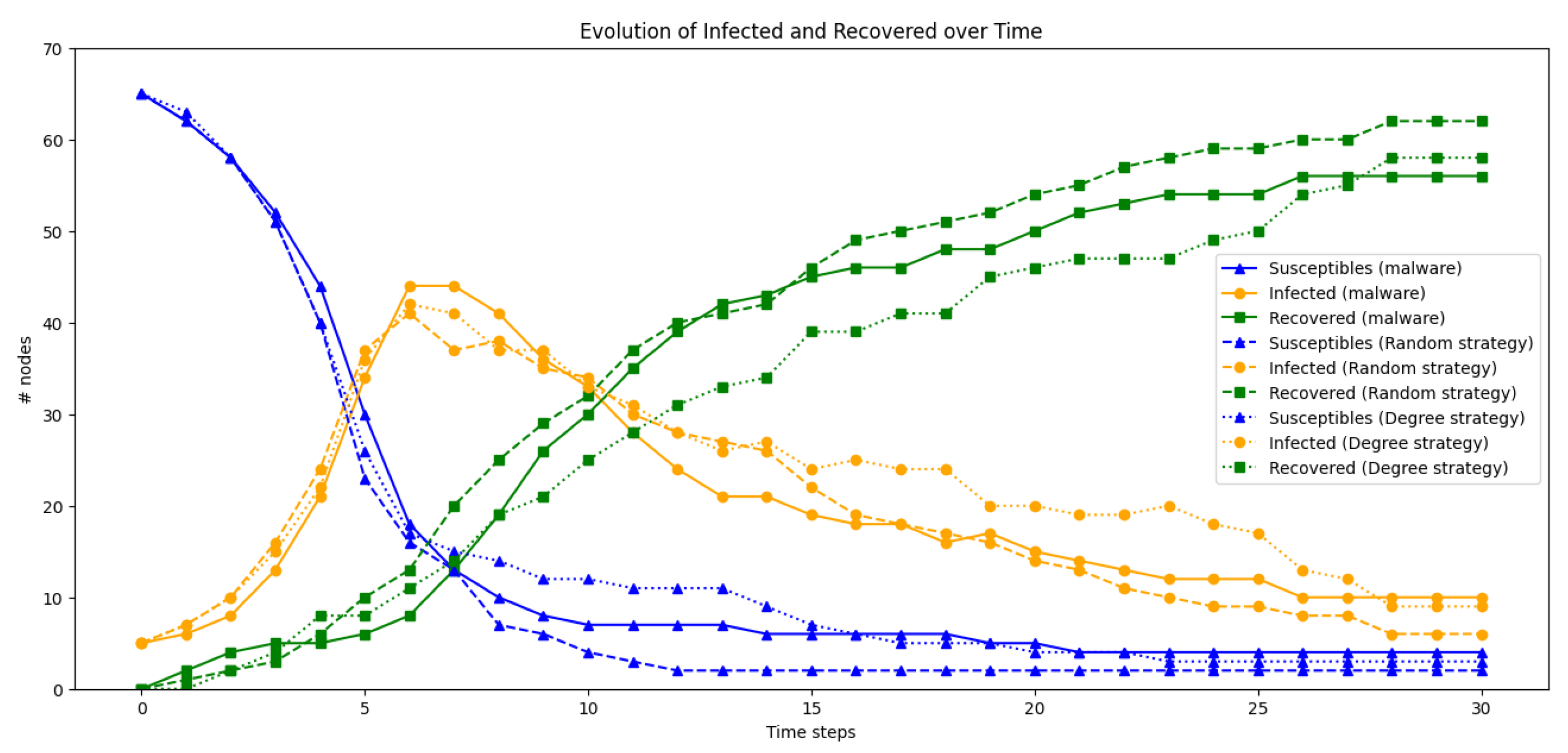
4.2.3. Simulation 1.3 with Nodes, Patching , Early Patching Time Step
4.2.4. Simulation 2.1 with Nodes, Patching , Early Patching Time Step
4.2.5. Simulation 2.2 with Nodes, Patching , Early Patching Time Step
4.2.6. Simulation 2.3 with Nodes, Patching , Early Patching Time Step
5. Conclusions
Author Contributions
Funding
Data Availability Statement
Conflicts of Interest
References
- Stoyanova, M.; Nikoloudakis, Y.; Panagiotakis, S.; Pallis, E.; Markakis, E.K. A survey on the internet of things (IoT) forensics: Challenges, approaches, and open issues. IEEE Commun. Surv. Tutor. 2020, 22, 1191–1221. [Google Scholar] [CrossRef]
- Xie, H.; Qin, Z. A lite distributed semantic communication system for Internet of Things. IEEE J. Sel. Areas Commun. 2020, 39, 142–153. [Google Scholar] [CrossRef]
- Wang, X.; Zhang, X.; Wang, S.; Xiao, J.; Tao, X. Modeling, Critical Threshold, and Lowest-Cost Patching Strategy of Malware Propagation in Heterogeneous IoT Networks. IEEE Trans. Inf. Forensics Secur. 2023, 18, 3531–3545. [Google Scholar] [CrossRef]
- Swessi, D.; Idoudi, H. A survey on internet-of-things security: Threats and emerging countermeasures. Wirel. Pers. Commun. 2022, 124, 1557–1592. [Google Scholar] [CrossRef]
- Xu, D.; Wang, X.; Hao, Y.; Zhang, Z.; Hao, Q.; Zhou, Z. A More Accurate and Robust Binary Ring-LWE Decryption Scheme and Its Hardware Implementation for IoT Devices. IEEE Trans. Very Large Scale Integr. VLSI Syst. 2022, 30, 1007–1019. [Google Scholar] [CrossRef]
- Zografopoulos, I.; Hatziargyriou, N.D.; Konstantinou, C. Distributed energy resources cybersecurity outlook: Vulnerabilities, attacks, impacts, and mitigations. IEEE Syst. J. 2023, 17, 6695–6709. [Google Scholar] [CrossRef]
- Ahmad, S.; Jha, S.; Alam, A.; Alharbi, M.; Nazeer, J. Analysis of intrusion detection approaches for network traffic anomalies with comparative analysis on botnets (2008–2020). Secur. Commun. Netw. 2022, 2022, 9199703. [Google Scholar] [CrossRef]
- Antonakakis, M.; April, T.; Bailey, M.; Bernhard, M.; Bursztein, E.; Cochran, J.; Durumeric, Z.; Halderman, J.A.; Invernizzi, L.; Kallitsis, M.; et al. Understanding the mirai botnet. In Proceedings of the 26th USENIX Security Symposium (USENIX Security 17), Vancouver, BC, Canada, 16–18 August 2017; pp. 1093–1110. [Google Scholar]
- Güven, E.Y. Mirai Botnet Attack Detection in Low-Scale Network Traffic. Intell. Autom. Soft Comput. 2023, 37, 419–437. [Google Scholar] [CrossRef]
- James, A.V.; Sabitha, S. Malware attacks: A survey on mitigation measures. In Proceedings of the Second International Conference on Networks and Advances in Computational Technologies: NetACT 19; Springer: Cham, Switzerland, 2021; pp. 1–11. [Google Scholar]
- Pachhala, N.; Jothilakshmi, S.; Battula, B.P. A comprehensive survey on identification of malware types and malware classification using machine learning techniques. In Proceedings of the 2021 2nd International Conference on Smart Electronics and Communication (ICOSEC), Trichy, India, 7–9 October 2021; pp. 1207–1214. [Google Scholar]
- Sprinkel, S.C. Global Internet Regulation: The Residual Effects of the ILoveYou Computer Virus and the Draft Convention on Cyber-Crime. Suffolk Transnat’L Rev. 2001, 25, 491. [Google Scholar]
- Zhang, C.; Zhou, S.; Chain, B.M. Hybrid epidemics—A case study on computer worm conficker. PloS ONE 2015, 10, e0127478. [Google Scholar] [CrossRef]
- Mohaisen, A.; Alrawi, O. Unveiling zeus: Automated classification of malware samples. In Proceedings of the 22nd International Conference on World Wide Web, Rio de Janeiro, Brazil, 13–17 May 2013; pp. 829–832. [Google Scholar]
- Sood, A.K.; Enbody, R.J.; Bansal, R. Dissecting SpyEye–Understanding the design of third generation botnets. Comput. Netw. 2013, 57, 436–450. [Google Scholar] [CrossRef]
- Thomas, K.; Bursztein, E.; Grier, C.; Ho, G.; Jagpal, N.; Kapravelos, A.; McCoy, D.; Nappa, A.; Paxson, V.; Pearce, P.; et al. Ad injection at scale: Assessing deceptive advertisement modifications. In Proceedings of the 2015 IEEE Symposium on Security and Privacy, San Jose, CA, USA, 17–21 May 2015; pp. 151–167. [Google Scholar]
- Mohurle, S.; Patil, M. A brief study of wannacry threat: Ransomware attack 2017. Int. J. Adv. Res. Comput. Sci. 2017, 8, 1938–1940. [Google Scholar]
- Mulligan, D.K.; Perzanowski, A.K. The magnificence of the disaster: Reconstructing the Sony BMG rootkit incident. Berkeley Technol. Law J. 2007, 22, 1157. [Google Scholar]
- Mannix, K.; Gorey, A.; O’Shea, D.; Newe, T. Sensor Network Environments: A Review of the Attacks and Trust Management Models for Securing Them. J. Sens. Actuator Netw. 2022, 11, 43. [Google Scholar] [CrossRef]
- Kermack, W.O.; McKendrick, A.G. A contribution to the mathematical theory of epidemics. Proc. R. Soc. London. Ser. Contain. Pap. Math. Phys. Character 1927, 115, 700–721. [Google Scholar]
- Shi, X.; Zhang, T.; Zhou, D.; Zhou, X. Dynamical analysis and optimal control of a stochastic SIAR model for computer viruses. Eur. Phys. J. Plus 2023, 138, 1–27. [Google Scholar] [CrossRef]
- She, B.; Gracy, S.; Sundaram, S.; Sandberg, H.; Johansson, K.H.; Paré, P.E. Epidemics spread over networks: Influence of infrastructure and opinions. In Cyber–Physical–Human Systems: Fundamentals and Applications; Wiley: Hoboken, NJ, USA, 2023; pp. 429–456. [Google Scholar]
- Morris, D.H.; Rossine, F.W.; Plotkin, J.B.; Levin, S.A. Optimal, near-optimal, and robust epidemic control. Commun. Phys. 2021, 4, 78. [Google Scholar] [CrossRef]
- Ojha, R.P.; Srivastava, P.K.; Sanyal, G.; Gupta, N. Improved model for the stability analysis of wireless sensor network against malware attacks. Wirel. Pers. Commun. 2021, 116, 2525–2548. [Google Scholar] [CrossRef]
- Gracy, S.; Wang, Y.; Pare, P.E.; Uribe, C.A. Multi-Competitive Virus Spread over a Time-Varying Networked SIS Model with an Infrastructure Network. arXiv 2023, arXiv:2303.08859. [Google Scholar] [CrossRef]
- Chen, J.; Huang, Y.; Zhang, R.; Zhu, Q. Optimal curing strategy for competing epidemics spreading over complex networks. IEEE Trans. Signal Inf. Process. Over Netw. 2021, 7, 294–308. [Google Scholar] [CrossRef]
- Dinakarrao, S.M.P.; Guo, X.; Sayadi, H.; Nowzari, C.; Sasan, A.; Rafatirad, S.; Zhao, L.; Homayoun, H. Cognitive and scalable technique for securing IoT networks against malware epidemics. IEEE Access 2020, 8, 138508–138528. [Google Scholar] [CrossRef]
- Khouzani, M.; Altman, E.; Sarkar, S. Optimal quarantining of wireless malware through power control. In Proceedings of the 2009 Information Theory and Applications Workshop, La Jolla, CA, USA, 8–13 February 2009; pp. 301–310. [Google Scholar]
- Shen, S.; Li, H.; Han, R.; Vasilakos, A.V.; Wang, Y.; Cao, Q. Differential game-based strategies for preventing malware propagation in wireless sensor networks. IEEE Trans. Inf. Forensics Secur. 2014, 9, 1962–1973. [Google Scholar] [CrossRef]
- Shen, S.; Ma, H.; Fan, E.; Hu, K.; Yu, S.; Liu, J.; Cao, Q. A non-cooperative non-zero-sum game-based dependability assessment of heterogeneous WSNs with malware diffusion. J. Netw. Comput. Appl. 2017, 91, 26–35. [Google Scholar] [CrossRef]
- Alamo, T.; Reina, D.G.; Gata, P.M.; Preciado, V.M.; Giordano, G. Data-driven methods for present and future pandemics: Monitoring, modelling and managing. Annu. Rev. Control. 2021, 52, 448–464. [Google Scholar] [CrossRef] [PubMed]
- Hong, Z.; Li, Y.; Gong, Y.; Chen, W. A data-driven spatially-specific vaccine allocation framework for COVID-19. Ann. Oper. Res. 2022, 1–24. [Google Scholar] [CrossRef]
- Castaneda, F.; Sezer, E.C.; Xu, J. Worm vs. worm: Preliminary study of an active counter-attack mechanism. In Proceedings of the 2004 ACM Workshop on Rapid Malcode, Washington, DC, USA, 20 October 2004; pp. 83–93. [Google Scholar]
- Musaddiq, A.; Zikria, Y.B.; Zulqarnain; Kim, S.W. Routing protocol for Low-Power and Lossy Networks for heterogeneous traffic network. EURASIP J. Wirel. Commun. Netw. 2020, 2020, 1–23. [Google Scholar] [CrossRef]
- Kuehne, H.; Jhuang, H.; Garrote, E.; Poggio, T.; Serre, T. HMDB: A large video database for human motion recognition. In Proceedings of the 2011 International Conference on Computer Vision, Barcelona, Spain, 6–13 November 2011; pp. 2556–2563. [Google Scholar]
- Roy, A.; Singh, C.; Narahari, Y. Recent advances in modeling and control of epidemics using a mean field approach. Sādhanā 2023, 48, 207. [Google Scholar] [CrossRef]
- Silva, D.H.; Anteneodo, C.; Ferreira, S.C. Epidemic outbreaks with adaptive prevention on complex networks. Commun. Nonlinear Sci. Numer. Simul. 2023, 116, 106877. [Google Scholar] [CrossRef]
- Maitra, U.; Hota, A.R.; Srivastava, V. SIS Epidemic Propagation under Strategic Non-myopic Protection: A Dynamic Population Game Approach. IEEE Control Syst. Lett. 2023, 7, 1578–1583. [Google Scholar] [CrossRef]
- Hota, A.R.; Maitra, U.; Elokda, E.; Bolognani, S. Learning to Mitigate Epidemic Risks: A Dynamic Population Game Approach. Dyn. Games Appl. 2023, 13, 1106–1129. [Google Scholar] [CrossRef]
- Hassan, R.; Rafatirad, S.; Homayoun, H.; Dinakarrao, S.M.P. Performance-aware Malware Epidemic Confinement in Large-Scale IoT Networks. In Proceedings of the ICC 2021-IEEE International Conference on Communications, Montreal, QC, Canada, 14–23 June 2021; pp. 1–6. [Google Scholar]
- Yang, L.X.; Li, P.; Yang, X.; Xiang, Y.; Jiang, F.; Zhou, W. Effective Quarantine and Recovery Scheme Against Advanced Persistent Threat. IEEE Trans. Syst. Man Cybern. Syst. 2021, 51, 5977–5991. [Google Scholar] [CrossRef]
- Ren, J.; Zhang, C.; Hao, Q. A theoretical method to evaluate honeynet potency. Future Gener. Comput. Syst. 2021, 116, 76–85. [Google Scholar] [CrossRef]
- Farooq, M.J.; Zhu, Q. Modeling, analysis, and mitigation of dynamic botnet formation in wireless IoT networks. IEEE Trans. Inf. Forensics Secur. 2019, 14, 2412–2426. [Google Scholar] [CrossRef]
- Haghighi, M.S.; Wen, S.; Xiang, Y.; Quinn, B.; Zhou, W. On the race of worms and patches: Modeling the spread of information in wireless sensor networks. IEEE Trans. Inf. Forensics Secur. 2016, 11, 2854–2865. [Google Scholar] [CrossRef]
- Aman, M.N.; Javaid, U.; Sikdar, B. IoT-Proctor: A Secure and Lightweight Device Patching Framework for Mitigating Malware Spread in IoT Networks. IEEE Syst. J. 2022, 16, 3468–3479. [Google Scholar] [CrossRef]
- Marinov, T.T.; Marinova, R.S. Inverse problem for adaptive SIR model: Application to COVID-19 in Latin America. Infect. Dis. Model. 2022, 7, 134–148. [Google Scholar] [CrossRef] [PubMed]
- Murray, J.D. Mathematical biology: I. an introduction 2002. In Mathematical Biology: II. Spatial Models and Biomedical Applications; Springer: New York, NY, USA, 2003. [Google Scholar]
- Shafiq, M.; Gu, Z.; Cheikhrouhou, O.; Alhakami, W.; Hamam, H. The rise of “Internet of Things”: Review and open research issues related to detection and prevention of IoT-based security attacks. Wirel. Commun. Mob. Comput. 2022, 2022, 1–12. [Google Scholar] [CrossRef]
- del Rey, A.M.; Vara, R.C.; González, S.R. A computational propagation model for malware based on the SIR classic model. Neurocomputing 2022, 484, 161–171. [Google Scholar] [CrossRef]
- Erdos, P.; Rényi, A. On the evolution of random graphs. Publ. Math. Inst. Hung. Acad. 1960, 5, 17–60. [Google Scholar]
- Hagberg, A.; Swart, P.; Chult, D.S. Exploring Network Structure, Dynamics, and Function Using NetworkX; Technical Report; Los Alamos National Lab.(LANL): Los Alamos, NM, USA, 2008. [Google Scholar]
- Schiassi, E.; De Florio, M.; D’Ambrosio, A.; Mortari, D.; Furfaro, R. Physics-informed neural networks and functional interpolation for data-driven parameters discovery of epidemiological compartmental models. Mathematics 2021, 9, 2069. [Google Scholar] [CrossRef]
- Yuan, L.; Ni, Y.Q.; Deng, X.Y.; Hao, S. A-PINN: Auxiliary physics informed neural networks for forward and inverse problems of nonlinear integro-differential equations. J. Comput. Phys. 2022, 462, 111260. [Google Scholar] [CrossRef]
- Gao, H.; Zahr, M.J.; Wang, J.X. Physics-informed graph neural Galerkin networks: A unified framework for solving PDE-governed forward and inverse problems. Comput. Methods Appl. Mech. Eng. 2022, 390, 114502. [Google Scholar] [CrossRef]
- Grimm, V.; Heinlein, A.; Klawonn, A.; Lanser, M.; Weber, J. Estimating the time-dependent contact rate of SIR and SEIR models in mathematical epidemiology using physics-informed neural networks. Electron. Trans. Numer. Anal. 2022, 56, 1–27. [Google Scholar] [CrossRef]
- Raissi, M.; Perdikaris, P.; Karniadakis, G.E. Physics-informed neural networks: A deep learning framework for solving forward and inverse problems involving nonlinear partial differential equations. J. Comput. Phys. 2019, 378, 686–707. [Google Scholar] [CrossRef]
- Lu, L.; Meng, X.; Mao, Z.; Karniadakis, G.E. DeepXDE: A deep learning library for solving differential equations. SIAM Rev. 2021, 63, 208–228. [Google Scholar] [CrossRef]


| Mitigation Strategy | Reference | Advantages | Challenges |
|---|---|---|---|
| Optimal control | [36] |
|
|
| [37] |
|
| |
| [38] |
|
| |
| [39] |
|
| |
| Quarantine | [40] |
|
|
| [41] |
|
| |
| [40] |
|
| |
| [42] |
|
| |
| Patching | [43] |
|
|
| [44] |
|
| |
| [3] |
|
| |
| [45] |
|
|
| Hyperparameter | Value |
|---|---|
| Input neuron number | 1 |
| PINN input | (time, S(t), I(t), R(t))) |
| Output neuron number | 2 |
| PINN output | (global-,global-) |
| Hidden layers | 3 |
| Optimizer & LR | Adam with lr = 0.001 |
| Activation function | Tanh |
| Epochs | 20,000 |
| Simulation # | Metric | Malware without Mitigation | Malware with Mitigation and Random Node Selection | Malware with Mitigation and Degree Node Selection |
|---|---|---|---|---|
| Simulation 1.1 | Global infection rate patching strategy | 0.46 | 0.37 | 0.31 |
| Percentage of final susceptibles | 4.29 | 7.14 | 7.14 | |
| Average infection speed | 2.7 | 2.3 | 1.8 | |
| Std infection speed | 2.33 | 2.62 | 1.74 | |
| Var infection speed susceptibles | 5.41 | 6.88 | 3.03 | |
| Average recovery speed | 2.1 | 1.9 | 1.8 | |
| Std recovery speed | 1.6 | 1.72 | 1.6 | |
| Var recovery speed | 2.56 | 2.96 | 2.56 | |
| Simulation 1.2 | Global infection rate patching strategy | 0.44 | 0.28 | 0.23 |
| Percentage of final susceptibles | 0.0 | 8.57 | 10.0 | |
| Average infection speed | 2.67 | 2.27 | 2.17 | |
| Std infection speed | 3.06 | 2.88 | 2.74 | |
| Var infection speed susceptibles | 9.36 | 8.27 | 7.52 | |
| Average recovery speed | 1.9 | 1.87 | 1.87 | |
| Std recovery speed | 2.13 | 1.78 | 2.22 | |
| Var recovery speed | 4.56 | 3.18 | 4.92 | |
| Simulation 1.3 | Global infection rate patching strategy | 0.46 | 0.23 | 0.2 |
| Percentage of final susceptibles | 0.0 | 11.43 | 15.43 | |
| Average infection speed | 2.77 | 2.17 | 2.12 | |
| Std infection speed | 3.4 | 2.46 | 1.79 | |
| Var infection speed susceptibles | 11.58 | 6.07 | 5.21 | |
| Average recovery speed | 2.0 | 1.73 | 1.67 | |
| Std recovery speed | 1.95 | 1.53 | 1.48 | |
| Var recovery speed | 3.8 | 2.33 | 2.18 |
| Simulation # | Metric | Malware without Mitigation | Malware with Mitigation and Random Node Selection | Malware with Mitigation and Degree Node Selection |
|---|---|---|---|---|
| Simulation 2.1 | Global infection rate patching strategy | 0.43 | 0.35 | 0.3 |
| Percentage of final susceptibles | 0.0 | 4.29 | 12.86 | |
| Average infection speed | 2.57 | 2.07 | 1.73 | |
| Std infection speed | 3.06 | 2.16 | 1.24 | |
| Var infection speed susceptibles | 9.38 | 4.66 | 1.53 | |
| Average recovery speed | 1.8 | 1.8 | 1.8 | |
| Std recovery speed | 1.87 | 1.49 | 1.17 | |
| Var recovery speed | 3.49 | 2.23 | 1.36 | |
| Simulation 2.2 | Global infection rate patching strategy | 0.48 | 0.4 | 0.34 |
| Percentage of final susceptibles | 4.29 | 4.29 | 4.29 | |
| Average infection speed | 2.07 | 2.03 | 1.83 | |
| Std infection speed | 2.28 | 2.69 | 2.28 | |
| Var infection speed susceptibles | 5.2 | 7.23 | 5.21 | |
| Average recovery speed | 1.87 | 1.83 | 1.77 | |
| Std recovery speed | 1.61 | 1.53 | 1.61 | |
| Var recovery speed | 2.58 | 2.34 | 2.58 | |
| Simulation 2.3 | Global infection rate patching strategy | 0.45 | 0.37 | 0.32 |
| Percentage of final susceptibles | 5.71 | 2.86 | 2.79 | |
| Average infection speed | 2.5 | 2.43 | 2.53 | |
| Std infection speed | 3.11 | 2.67 | 2.81 | |
| Var infection speed susceptibles | 9.65 | 7.11 | 7.92 | |
| Average recovery speed | 1.87 | 2.07 | 1.93 | |
| Std recovery speed | 1.91 | 1.71 | 1.59 | |
| Var recovery speed | 3.65 | 2.93 | 2.53 |
Disclaimer/Publisher’s Note: The statements, opinions and data contained in all publications are solely those of the individual author(s) and contributor(s) and not of MDPI and/or the editor(s). MDPI and/or the editor(s) disclaim responsibility for any injury to people or property resulting from any ideas, methods, instructions or products referred to in the content. |
© 2024 by the authors. Licensee MDPI, Basel, Switzerland. This article is an open access article distributed under the terms and conditions of the Creative Commons Attribution (CC BY) license (https://creativecommons.org/licenses/by/4.0/).
Share and Cite
Casado-Vara, R.; Severt, M.; Díaz-Longueira, A.; Rey, Á.M.d.; Calvo-Rolle, J.L. Dynamic Malware Mitigation Strategies for IoT Networks: A Mathematical Epidemiology Approach. Mathematics 2024, 12, 250. https://doi.org/10.3390/math12020250
Casado-Vara R, Severt M, Díaz-Longueira A, Rey ÁMd, Calvo-Rolle JL. Dynamic Malware Mitigation Strategies for IoT Networks: A Mathematical Epidemiology Approach. Mathematics. 2024; 12(2):250. https://doi.org/10.3390/math12020250
Chicago/Turabian StyleCasado-Vara, Roberto, Marcos Severt, Antonio Díaz-Longueira, Ángel Martín del Rey, and Jose Luis Calvo-Rolle. 2024. "Dynamic Malware Mitigation Strategies for IoT Networks: A Mathematical Epidemiology Approach" Mathematics 12, no. 2: 250. https://doi.org/10.3390/math12020250
APA StyleCasado-Vara, R., Severt, M., Díaz-Longueira, A., Rey, Á. M. d., & Calvo-Rolle, J. L. (2024). Dynamic Malware Mitigation Strategies for IoT Networks: A Mathematical Epidemiology Approach. Mathematics, 12(2), 250. https://doi.org/10.3390/math12020250