Fekete–Szegő and Zalcman Functional Estimates for Subclasses of Alpha-Convex Functions Related to Trigonometric Functions ^†

Abstract

In this study, we introduce the new subclasses, ${\mathcal{M}}_{\alpha }(sin)$ and ${\mathcal{M}}_{\alpha }(cos)$, of $\alpha$-convex functions associated with sine and cosine functions. First, we obtain the initial coefficient bounds for the first five coefficients of the functions that belong to these classes. Further, we determine the upper bound of the Zalcman functional for the class ${\mathcal{M}}_{\alpha }(cos)$ for the case $n=3$, proving that the Zalcman conjecture holds for this value of n. Moreover, the problem of the Fekete–Szegő functional estimate for these classes is studied.

1. Introduction and Preliminaries

Let $\mathcal{T}$ be the class consisting of all analytic and normalized functions f, where f has the Taylor expansion of the form

$$f\left(z\right)=z+a_2{z}^2+a_3{z}^3+\cdots ,z\in \mathbb{D},$$

(1)

and $\mathbb{D}:=\left\{z\in \mathbb{C}:\left|z\right|<1\right\}$ is the open unit disk; also, the subclass of $\mathcal{T}$ consisting of univalent functions is denoted by $\mathcal{S}$.

Let us consider two analytic functions, $\mathrm{P}$ and $\mathrm{Q}$, in $\mathbb{D}$. The function $\mathrm{P}$ is said to be subordinated to $\mathrm{Q}$, written symbolically as $\mathrm{P}\left(z\right)\prec \mathrm{Q}\left(z\right)$, if there exists an analytic function $\eta$ in $\mathbb{D}$, with $\eta \left(0\right)=0$ and $\left|\eta \right(z\left)\right|<1$ for all $z\in \mathbb{D}$, such that $\mathrm{P}=\mathrm{Q}\circ \eta$. In addition, if $\mathrm{Q}$ is an univalent function in $\mathbb{D}$, then the following equivalence holds (see [1]):

$$\mathrm{P}\left(z\right)\prec \mathrm{Q}\left(z\right)\iff \mathrm{P}\left(0\right)=\mathrm{Q}\left(0\right)\mathrm{and}\mathrm{P}\left(\mathbb{D}\right)\subset \mathrm{Q}\left(\mathbb{D}\right).$$

The family of functions p analytic in $\mathbb{D}$ satisfying the condition $Rep\left(z\right)>0$, $z\in \mathbb{D}$, and of the form

$$p\left(z\right)=1+\sum _{n=1}^{\infty }{t}_n{z}^n,z\in \mathbb{D},$$

(2)

is denoted by $\mathcal{P}$, which represents the well-known Carathéodory function class.

In [2], Mocanu introduced and studied the well-known class of α-convex functions, that is

$${\mathcal{M}}_{\alpha }:=\left\{f\in \mathcal{T}:Re\left[\left(1-\alpha \right){\displaystyle \frac{z{f}^{\prime }\left(z\right)}{f\left(z\right)}}+\alpha \left(1+\frac{z{f}^{\prime \prime }\left(z\right)}{f^{\prime }\left(z\right)}\right)\right]>0,z\in \mathbb{D}\right\},\alpha \ge 0,$$

and the properties of this class of functions were extensively studied during a long period by many researchers (see, for example [3,4,5]). In [6], it was proved that all $\alpha$-convex functions are univalent and starlike, while the subclass ${\mathcal{S}}^{*}:={\mathcal{M}}_0$ is called the class of starlike (normalized) functions in $\mathbb{D}$ and ${\mathcal{S}}^c:={\mathcal{M}}_1$ represents the class of convex (normalized) functions in $\mathbb{D}$.

Note that a function is considered starlike in $\mathbb{D}$ if it is univalent in $\mathbb{D}$ and maps the open unit disk onto a starlike domain, while it is convex in $\mathbb{D}$ if it is univalent in $\mathbb{D}$ and maps the open unit disk onto a convex domain. Therefore, the $\alpha$-convex functions extend both of these two classes, and make a “continuous” transition between these remarkable classes (for details see [2,6]). We would like to emphasize that the notion of subordination plays an important role in Geometric Function Theory because of the above equivalence that deals with the range of the open unit disk $\mathbb{D}$ by the function Q. Thus, for a function $p\in \mathcal{P}$ if and only if $p\left(z\right)\prec {\displaystyle \frac{1+z}{1-z}}=:\chi \left(z\right)$, and for a function $f\in \mathcal{T}$, we have the equivalences

$$f\in {\mathcal{S}}^{*}\iff {\displaystyle \frac{z{f}^{\prime }\left(z\right)}{f\left(z\right)}}\prec \chi \left(z\right),f\in {\mathcal{S}}^c\iff 1+\frac{z{f}^{\prime \prime }\left(z\right)}{f^{\prime }\left(z\right)}\prec \chi \left(z\right),$$

while

$${\mathcal{M}}_{\alpha }=\left\{f\in \mathcal{T}:\left(1-\alpha \right){\displaystyle \frac{z{f}^{\prime }\left(z\right)}{f\left(z\right)}}+\alpha \left(1+\frac{z{f}^{\prime \prime }\left(z\right)}{f^{\prime }\left(z\right)}\right)\prec \chi \left(z\right)\right\},\alpha \ge 0.$$

Definition 1.

Let us define the new classes, ${\mathcal{M}}_{\alpha }(sin)$ and ${\mathcal{M}}_{\alpha }(cos)$, with $\alpha \ge 0$, connected with the sine and cosine functions, respectively, as follows:

$$\begin{array}{ccc}& & {\mathcal{M}}_{\alpha }(sin):=\left\{f\in \mathcal{T}:\left(1-\alpha \right){\displaystyle \frac{z{f}^{\prime }\left(z\right)}{f\left(z\right)}}+\alpha \left(1+\frac{z{f}^{\prime \prime }\left(z\right)}{f^{\prime }\left(z\right)}\right)\prec 1+sinz=:\mathrm{\Phi }\left(z\right)\right\},\hfill \end{array}$$

(3)

$$\begin{array}{ccc}& & {\mathcal{M}}_{\alpha }(cos):=\left\{f\in \mathcal{T}:\left(1-\alpha \right){\displaystyle \frac{z{f}^{\prime }\left(z\right)}{f\left(z\right)}}+\alpha \left(1+\frac{z{f}^{\prime \prime }\left(z\right)}{f^{\prime }\left(z\right)}\right)\prec cosz=:\mathrm{\Psi }\left(z\right)\right\}.\hfill \end{array}$$

(4)

Remark 1.

(i) 

Substituting the value of $\alpha =0$ and $\alpha =1$ in (3), we obtain the following subclasses which were studied in [7,8,9], respectively, that are

$${\mathcal{S}}_{sin}^{*}:={\mathcal{M}}_0\left(sin\right),{\mathcal{S}}_{sin}^c:={\mathcal{M}}_1\left(sin\right).$$

(ii) 

Taking $\alpha =0$ in (4) we obtain the subclass ${\mathcal{S}}_{cos}^{*}:={\mathcal{M}}_0\left(cos\right)$ defined in [10], and by taking $\alpha =1$ in (4) we obtain the subclass ${\mathcal{S}}_{cos}^c:={\mathcal{M}}_1\left(cos\right)$. An extensive study of the estimations of the first seven coefficients, of some Hankel determinants, of the Zalcman conjecture and of the logarithmic coefficients for these two subclasses was recently given in [11].

Thus, it could be seen that the function classes defined by (3) and (4) extend some previous classes defined by different authors.

(iii) 

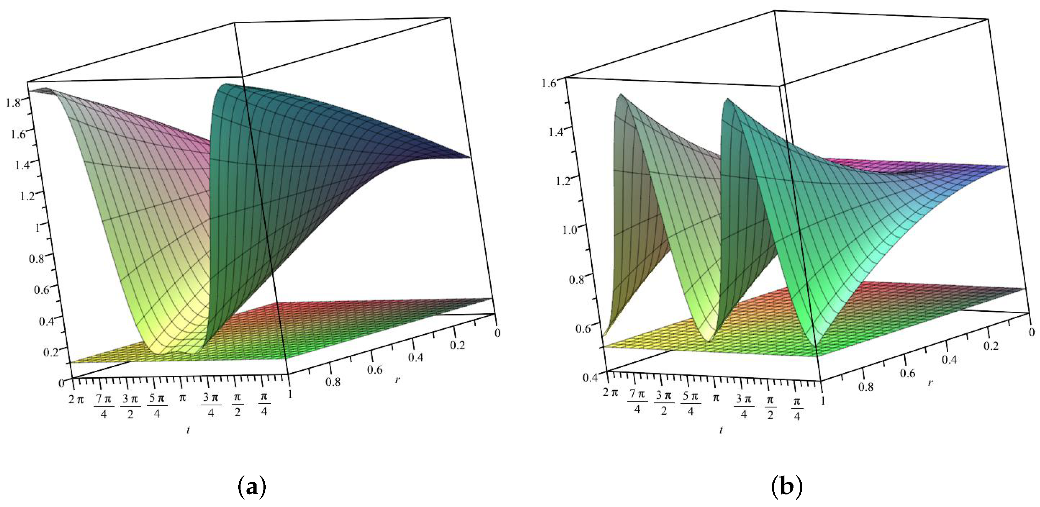
Since the functions Φ and Ψ defined above have real positive parts in $\mathbb{D}$, and, moreover, (see the Figure 1a,b, made with MAPLE 2023™ computer software)

$$Re\mathrm{\Phi }\left(z\right)>\frac{1}{10},Re\mathrm{\Psi }\left(z\right)>\frac{1}{2},z\in \mathbb{D},$$

it follows that the classes ${\mathcal{M}}_{\alpha }(sin)$ and ${\mathcal{M}}_{\alpha }(cos)$ are subsets of the class ${\mathcal{M}}_{\alpha }$, that is ${\mathcal{M}}_{\alpha }(sin),{\mathcal{M}}_{\alpha }(cos)\subset {\mathcal{M}}_{\alpha }\subset {\mathcal{S}}^{*}\subset \mathcal{S}$, $\alpha \ge 0$.

The following lemmas are necessary in the proof of our main results.

Lemma 1.

If $p\in \mathcal{P}$ has the form (2), then

$$\begin{array}{ccc}& & |t_n|\le 2,forn\ge 1,\hfill \end{array}$$

(5)

$$\begin{array}{ccc}& & |t_{i+j}-\mu t_i{t}_j|\le 2max\{1;|1-2\mu |\},for\mu \in \mathbb{C},\hfill \end{array}$$

(6)

and for any number $\zeta \in \mathbb{C}$ we have

$$|t_2-\zeta t_1^2|\le 2max\left\{1;|2\zeta -1|\right\}.$$

(7)

The inequality (5) is the well-known Carathéodory’s result (see [12,13]), while (6) may be found in [1], and the inequality (7) is from [14] (see also [15] [Lemma 2]).

Lemma 2

([7] Lemma 2.2). If $p\in \mathcal{P}$ has the form (2), then

$$|\alpha t_1^3-\beta t_1{t}_2+\gamma t_3|\le 2|\alpha |+2|\beta -2\alpha |+2|\alpha -\beta +\gamma |.$$

(8)

2. Initial Coefficient Estimates for the Classes ${\mathcal{M}}_{\mathit{\alpha }}\left(\mathbf{s}\mathbf{i}\mathbf{n}\right)$ and ${\mathcal{M}}_{\mathit{\alpha }}\left(\mathbf{c}\mathbf{o}\mathbf{s}\right)$

In this section, the coefficients of the functions of the classes ${\mathcal{M}}_{\alpha }(sin)$ and ${\mathcal{M}}_{\alpha }(cos)$ are analysed, and the upper bounds for the first five coefficients are obtained.

Theorem 1.

If $f\in {\mathcal{M}}_{\alpha }(sin)$ has the form (1), then

$$\begin{array}{cc}\hfill |a_2|\le & \frac{1}{1+\alpha },\hfill \\ \hfill |a_3|\le & \frac{1}{2\left(1+2\alpha \right)}max\left\{1;\frac{3\alpha +1}{{\left(1+\alpha \right)}^2}\right\},\hfill \\ \hfill |a_4|\le & \frac{1}{6\left(1+3\alpha \right)}\left(max\left\{1;{\displaystyle \frac{6\alpha (\alpha -1)}{\left(1+2\alpha \right)\left(1+\alpha \right)}}\right\}+{\displaystyle \frac{-4{\alpha }^4+31{\alpha }^3+30{\alpha }^2+35\alpha +4}{3\left(1+2\alpha \right){\left(1+\alpha \right)}^3}}\right),\hfill \\ \hfill |a_5|\le & \frac{1}{4\left(1+4\alpha \right)}[\frac{1}{2}\left(max\left\{1;\frac{\left|27{\alpha }^2-20\alpha +1\right|}{9{\alpha }^2+12\alpha +3}\right\}+1\right)\hfill \\ \hfill & +\frac{|{\mathrm{\Phi }}_1\left(\alpha \right)\left|\right|{\mathrm{\Phi }}_2\left(\alpha \right)|}{18\left(1+3\alpha \right){\left(1+2\alpha \right)}^2{\left(1+\alpha \right)}^2}+\mathrm{M}\left(\alpha \right)],\hfill \end{array}$$

where

$$\begin{array}{cc}\hfill {\mathrm{\Phi }}_1\left(\alpha \right)& :=-108{\alpha }^7+200{\alpha }^6+556{\alpha }^5+1042{\alpha }^4+631{\alpha }^3+409{\alpha }^2+145\alpha +5,\hfill \\ \hfill {\mathrm{\Phi }}_2\left(\alpha \right)& :=-180{\alpha }^5-8{\alpha }^4+69{\alpha }^3+187{\alpha }^2+75\alpha +1,\hfill \end{array}$$

and

$$\mathrm{M}\left(\alpha \right):=\frac{8{\alpha }^2+1}{9{\left(1+2\alpha \right)}^2}max\left\{1;\left|1-\frac{{\mathrm{\Phi }}_2\left(\alpha \right)}{\left(1+3\alpha \right){\left(1+\alpha \right)}^2\left(8{\alpha }^2+1\right)}\right|\right\}.$$

Proof. 

If $f\in {\mathcal{M}}_{\alpha }(sin)$, then there exists a function $\eta$ that is analytic in $\mathbb{D}$ and satisfies the conditions $\eta \left(0\right)=0$ and $\left|\eta \right(z\left)\right|<1$ for all $z\in \mathbb{D}$, such that

$$\left(1-\alpha \right){\displaystyle \frac{z{f}^{\prime }\left(z\right)}{f\left(z\right)}}+\alpha \left(1+\frac{z{f}^{\prime \prime }\left(z\right)}{f^{\prime }\left(z\right)}\right)=\mathrm{\Phi }\left(\eta \left(z\right)\right)=1+sin\eta \left(z\right),z\in \mathbb{D}.$$

Since f is of the form (1), it follows that

$$\begin{array}{cc}\hfill \left(1-\alpha \right){\displaystyle \frac{z{f}^{\prime }\left(z\right)}{f\left(z\right)}}+\alpha \left(1+\frac{z{f}^{\prime \prime }\left(z\right)}{f^{\prime }\left(z\right)}\right)=& 1+\left(1+\alpha \right)a_{2}z+\left(-3\alpha a_2^2+4\alpha a_3-a_2^2+2a_3\right)z^2\hfill \\ \hfill & +\left(7\alpha a_2^3-15\alpha a_2{a}_3+a_2^3+9\alpha a_4-3a_2{a}_3+3a_4\right)z^3\hfill \\ \hfill & +\left(-15\alpha a_2^4+44\alpha a_2^2{a}_3-a_2^4-28\alpha a_2{a}_4-16\alpha a_3^2\right.\hfill \\ \hfill & \left.+4a_2^2{a}_3+16\alpha a_5-4a_2{a}_4-2a_3^2+4a_5\right)z^4+\cdots ,z\in \mathbb{D}.\hfill \end{array}$$

(9)

From the fact that $\eta \left(0\right)=0$ and $\left|\eta \right(z\left)\right|<1$ for all $z\in \mathbb{D}$, if we define the function p by

$$p\left(z\right):=\frac{1+\eta \left(z\right)}{1-\eta \left(z\right)}=1+t_{1}z+t_2{z}^2+\cdots ,z\in \mathbb{D},$$

we obtain that $p\in \mathcal{P}$ and

$$\eta \left(z\right)=\frac{p\left(z\right)-1}{p\left(z\right)+1}=\frac{t_{1}z+t_2{z}^2+\cdots }{2+t_{1}z+t_2{z}^2+\cdots },z\in \mathbb{D}.$$

According to the above relation, we obtain

$$\begin{array}{cc}\hfill 1+sin\eta \left(z\right)=& 1+\frac{1}{2}{t}_{1}z+\left(\frac{t_2}{2}-\frac{t_1^2}{4}\right)z^2+\left(\frac{1}{2}{t}_3-\frac{1}{2}{t}_1{t}_2+\frac{5}{48}{t}_1^3\right)z^3\hfill \\ \hfill & +\left(\frac{5}{16}{t}_2{t}_1^2-\frac{1}{32}{t}_1^4+\frac{1}{2}{t}_4-\frac{1}{2}{t}_1{t}_3-\frac{1}{4}{t}_2^2\right)z^4+\cdots ,z\in \mathbb{D},\hfill \end{array}$$

(10)

$$\begin{array}{cc}\hfill cos\eta \left(z\right)=& 1-\frac{t_1^2}{8}{z}^2+\left(-\frac{1}{4}{t}_1{t}_2+\frac{1}{8}{t}_1^3\right)z^3\hfill \\ \hfill & +\left(-\frac{35}{384}{t}_1^4-\frac{1}{8}{t}_2^2+\frac{3}{8}{t}_2{t}_1^2-\frac{1}{4}{t}_1{t}_3\right)z^4+\cdots ,z\in \mathbb{D},\hfill \end{array}$$

(11)

and equating the corresponding coefficients of (9) and (10) we obtain

$$\begin{array}{cc}\hfill a_2=& \frac{t_1}{2(1+\alpha )},\hfill \end{array}$$

(12)

$$\begin{array}{cc}\hfill a_3=& \frac{2{\left(1+\alpha \right)}^2{t}_2+\alpha \left(1-\alpha \right)t_1^2}{8\left(1+2\alpha \right){\left(1+\alpha \right)}^2},\hfill \end{array}$$

(13)

$$\begin{array}{cc}\hfill a_4=& \frac{5\left(1+2\alpha \right){\left(1+\alpha \right)}^3-6\left(1+7\alpha \right)\left(1+2\alpha \right)+9\left(1+5\alpha \right)\left(1-\alpha \right)\alpha }{144\left(1+3\alpha \right)\left(1+2\alpha \right){\left(1+\alpha \right)}^3}{t}_1^3\hfill \\ \hfill & +\frac{6\left(1+5\alpha \right)-8\left(1+2\alpha \right)\left(1+\alpha \right)}{48\left(1+3\alpha \right)\left(1+2\alpha \right)\left(1+\alpha \right)}{t}_1{t}_2+\frac{1}{6\left(1+3\alpha \right)}{t}_3,\hfill \end{array}$$

(14)

$$\begin{array}{cc}\hfill a_5=& \frac{1}{4\left(1+4\alpha \right)}[\frac{{\mathrm{\Phi }}_1\left(\alpha \right)}{288\left(1+3\alpha \right){\left(1+2\alpha \right)}^2{\left(1+\alpha \right)}^4}{t}_1^4-\frac{{\mathrm{\Phi }}_2\left(\alpha \right)}{48\left(1+3\alpha \right){\left(1+2\alpha \right)}^2{\left(1+\alpha \right)}^2}{t}_1^2{t}_2\hfill \\ \hfill & +\frac{2\left(1+7\alpha \right)-3\left(1+3\alpha \right)\left(1+\alpha \right)}{6\left(1+3\alpha \right)\left(1+\alpha \right)}{t}_1{t}_3+\frac{\left(1+8\alpha \right)-2{\left(1+2\alpha \right)}^2}{8{\left(1+2\alpha \right)}^2}{t}_2^2+\frac{1}{2}{t}_4].\hfill \end{array}$$

(15)

Using (12), we obtain

$$|a_2|=\frac{1}{2\left(1+\alpha \right)}\left|t_1\right|,$$

and from (5) we have $|t_1|\le 2$, hence

$$|a_2|\le \frac{1}{1+\alpha }.$$

The relation (13) leads to

$$|a_3|=\left|\frac{t_2}{4\left(1+2\alpha \right)}-\frac{\alpha \left(\alpha -1\right)t_1^2}{8\left(1+2\alpha \right){\left(1+\alpha \right)}^2}\right|,$$

using triangle inequality we obtain

$$|a_3|\le \frac{1}{4\left(1+2\alpha \right)}\left|t_2-\frac{\alpha \left(\alpha -1\right)t_1^2}{2{\left(1+\alpha \right)}^2}\right|,$$

and according to (7), since $\alpha \ge 0$, we obtain

$$\begin{array}{cc}\hfill |a_3|=\frac{1}{4\left(1+2\alpha \right)}\left|t_2-\frac{\alpha \left(\alpha -1\right)t_1^2}{2{\left(1+\alpha \right)}^2}\right|& \le \frac{1}{4\left(1+2\alpha \right)}2max\left\{1;\left|2·\frac{\alpha \left(\alpha -1\right)}{2{\left(1+\alpha \right)}^2}-1\right|\right\}\hfill \\ \hfill & =\frac{1}{2\left(1+2\alpha \right)}max\left\{1;\frac{3\alpha +1}{{\left(1+\alpha \right)}^2}\right\}.\hfill \end{array}$$

The equality (14) leads to

$$\begin{array}{cc}\hfill |a_4|=& \frac{1}{3\left(1+3\alpha \right)}\left|\frac{1}{4}\left(t_3-\frac{4\left(1+2\alpha \right)\left(1+\alpha \right)-3\left(1+5\alpha \right)}{2\left(1+2\alpha \right)\left(1+\alpha \right)}{t}_1{t}_2\right)\right.\hfill \\ \hfill & \left.+\frac{t_3}{4}-\frac{6\left(1+7\alpha \right)\left(1+2\alpha \right)-5\left(1+2\alpha \right){\left(1+\alpha \right)}^3-9\left(1+5\alpha \right)\left(1-\alpha \right)\alpha }{12\left(1+2\alpha \right){\left(1+\alpha \right)}^3}{t}_1^3\right|,\hfill \end{array}$$

and using the triangle inequality we obtain

$$\begin{array}{cc}\hfill |a_4|\le & \frac{1}{3\left(1+3\alpha \right)}[\frac{1}{4}\left|t_3-\frac{4\left(1+2\alpha \right)\left(1+\alpha \right)-3\left(1+5\alpha \right)}{2\left(1+2\alpha \right)\left(1+\alpha \right)}{t}_1{t}_2\right|\hfill \\ \hfill & +\frac{|t_3|}{4}+\frac{6\left(1+7\alpha \right)\left(1+2\alpha \right)-5\left(1+2\alpha \right){\left(1+\alpha \right)}^3-9\left(1+5\alpha \right)\left(1-\alpha \right)\alpha }{12\left(1+2\alpha \right){\left(1+\alpha \right)}^3}{\left|t_1\right|}^3].\hfill \end{array}$$

From (5) and (6), the above inequality implies that

$$\begin{array}{cc}\hfill |a_4|\le & \frac{1}{6\left(1+3\alpha \right)}\left(max\left\{1;{\displaystyle \frac{6\alpha (\alpha -1)}{\left(1+2\alpha \right)\left(1+\alpha \right)}}\right\}+{\displaystyle \frac{-4{\alpha }^4+31{\alpha }^3+30{\alpha }^2+35\alpha +4}{3\left(1+2\alpha \right){\left(1+\alpha \right)}^3}}\right).\hfill \end{array}$$

By rearranging (15) we obtain

$$\begin{array}{cc}\hfill |a_5|=& \frac{1}{4\left(1+4\alpha \right)}|\frac{1}{4}\left(t_4-\frac{6\left(1+3\alpha \right)\left(1+\alpha \right)-4\left(1+7\alpha \right)}{3\left(1+3\alpha \right)\left(1+\alpha \right)}{t}_1{t}_3\right)\hfill \\ \hfill & +\frac{1}{4}\left(t_4-\frac{-7\left(\left(1+8\alpha \right)-2{\left(1+2\alpha \right)}^2\right)}{18{\left(1+2\alpha \right)}^2}{t}_2^2\right)\hfill \\ \hfill & -\frac{5{\mathrm{\Phi }}_2\left(\alpha \right)}{144\left(1+3\alpha \right){\left(1+2\alpha \right)}^2{\left(1+\alpha \right)}^2}{t}_1^2{t}_2+\frac{{\mathrm{\Phi }}_1\left(\alpha \right)}{288\left(1+3\alpha \right){\left(1+2\alpha \right)}^2{\left(1+\alpha \right)}^4}{t}_1^4\hfill \\ \hfill & -\frac{2{\left(1+2\alpha \right)}^2-\left(1+8\alpha \right)}{36{\left(1+2\alpha \right)}^2}{t}_2\left(t_2-\frac{{\mathrm{\Phi }}_2\left(\alpha \right)}{2\left(1+3\alpha \right){\left(1+\alpha \right)}^2\left(2{\left(1+2\alpha \right)}^2-\left(1+8\alpha \right)\right)}{t}_1^2\right)|,\hfill \end{array}$$

and using triangle inequality we obtain

$$\begin{array}{cc}\hfill |a_5|\le & \frac{1}{4\left(1+4\alpha \right)}[\frac{1}{4}\left|t_4-\frac{6\left(1+3\alpha \right)\left(1+\alpha \right)-4\left(1+7\alpha \right)}{3\left(1+3\alpha \right)\left(1+\alpha \right)}{t}_1{t}_3\right|\hfill \\ \hfill & +\frac{1}{4}\left|t_4-\frac{7\left(2{\left(1+2\alpha \right)}^2-\left(1+8\alpha \right)\right)}{18{\left(1+2\alpha \right)}^2}{t}_2^2\right|\hfill \\ \hfill & +\frac{5|{\mathrm{\Phi }}_2\left(\alpha \right)|}{144\left(1+3\alpha \right){\left(1+2\alpha \right)}^2{\left(1+\alpha \right)}^2}|t_1{|}^2|t_2|+\frac{|{\mathrm{\Phi }}_1\left(\alpha \right)|}{288\left(1+3\alpha \right){\left(1+2\alpha \right)}^2{\left(1+\alpha \right)}^4}{\left|t_1\right|}^4\hfill \\ \hfill & +\frac{8{\alpha }^2+1}{36{\left(1+2\alpha \right)}^2}\left|t_2\right||t_2-\frac{{\mathrm{\Phi }}_2\left(\alpha \right)}{2\left(1+3\alpha \right){\left(1+\alpha \right)}^2\left(8{\alpha }^2+1)\right)}{t}_1^2|].\hfill \end{array}$$

(16)

Now, we will find an upper bound for the each term of the right hand side of the above inequality, as follows.

(i)

According to (6), we have

$$\begin{array}{cc}\hfill \left|t_4-\frac{6\left(1+3\alpha \right)\left(1+\alpha \right)-4\left(1+7\alpha \right)}{3\left(1+3\alpha \right)\left(1+\alpha \right)}{t}_1{t}_3\right|& \le 2max\left\{1;\left|1-\frac{12\left(1+3\alpha \right)\left(1+\alpha \right)-8\left(1+7\alpha \right)}{3\left(1+3\alpha \right)\left(1+\alpha \right)}\right|\right\}\hfill \\ \hfill & =2max\left\{1;\left|\frac{27{\alpha }^2-20\alpha +1}{9{\alpha }^2+12\alpha +3}\right|\right\},\hfill \end{array}$$

whenever $\alpha \ge 0$.

(ii)

Using, again, the inequality (6), a simple computation shows that

$$\begin{array}{cc}\hfill \left|t_4-\frac{7\left(2{\left(1+2\alpha \right)}^2-\left(1+8\alpha \right)\right)}{18{\left(1+2\alpha \right)}^2}{t}_2^2\right|& \le 2max\left\{1;\left|1-\frac{7\left(2{\left(1+2\alpha \right)}^2-\left(1+8\alpha \right)\right)}{9{\left(1+2\alpha \right)}^2}\right|\right\}\hfill \\ \hfill & =2max\left\{1;\left|\frac{2(10{\alpha }^2-18\alpha -1)}{9{\left(1+2\alpha \right)}^2}\right|\right\}=2,\hfill \end{array}$$

whenever $\alpha \ge 0$.

(iii)

For the sum of the third with the fourth term, using inequality (5), we obtain

$$\begin{array}{c}\hfill \frac{5|{\mathrm{\Phi }}_2\left(\alpha \right)|}{144\left(1+3\alpha \right){\left(1+2\alpha \right)}^2{\left(1+\alpha \right)}^2}|t_1{|}^2|t_2|+\frac{|{\mathrm{\Phi }}_1\left(\alpha \right)|}{288\left(1+3\alpha \right){\left(1+2\alpha \right)}^2{\left(1+\alpha \right)}^4}{\left|t_1\right|}^4\\ \hfill \le \frac{|{\mathrm{\Phi }}_1\left(\alpha \right)\left|\right|{\mathrm{\Phi }}_2\left(\alpha \right)|}{18\left(1+3\alpha \right){\left(1+2\alpha \right)}^2{\left(1+\alpha \right)}^2}.\end{array}$$

(iv)

To get a majorant for the last term of the sum, according to (5) and (7), we have

$$\begin{array}{c}\hfill \frac{8{\alpha }^2+1}{36{\left(1+2\alpha \right)}^2}\left|t_2\right||t_2-\frac{{\mathrm{\Phi }}_2\left(\alpha \right)}{2\left(1+3\alpha \right){\left(1+\alpha \right)}^2\left(2{\left(1+2\alpha \right)}^2-\left(1+8\alpha \right)\right)}{t}_1^2|\}\\ \hfill \le \frac{8{\alpha }^2+1}{9{\left(1+2\alpha \right)}^2}max\left\{1;\left|1-\frac{{\mathrm{\Phi }}_2\left(\alpha \right)}{\left(1+3\alpha \right){\left(1+\alpha \right)}^2\left(8{\alpha }^2+1\right)}\right|\right\}:=M\left(\alpha \right).\end{array}$$

Finally, using the upper bounds found for the items (i)–(v), from the inequality (16) we conclude that

$$\begin{array}{cc}\hfill |a_5|\le & \frac{1}{4\left(1+4\alpha \right)}\{\frac{1}{2}\left(max\left\{1;\frac{\left|27{\alpha }^2-20\alpha +1\right|}{9{\alpha }^2+12\alpha +3}\right\}+1\right)\hfill \\ \hfill & +\frac{|{\mathrm{\Phi }}_1\left(\alpha \right)\left|\right|{\mathrm{\Phi }}_2\left(\alpha \right)|}{18\left(1+3\alpha \right){\left(1+2\alpha \right)}^2{\left(1+\alpha \right)}^2}+\mathrm{M}\left(\alpha \right)\}.\hfill \end{array}$$

□

Remark 2.

A simple computation shows that the upper bounds obtained in the Theorem 1 could be written in the following forms:

$$|a_3|\le \left\{\begin{array}{ccc}{\displaystyle \frac{3\alpha +1}{2(1+2\alpha ){(1+\alpha )}^2}},\hfill & if\hfill & 0\le \alpha \le 1,\hfill \\ {\displaystyle \frac{1}{2(1+2\alpha )}},\hfill & if\hfill & \alpha \ge 1,\hfill \end{array}\right.$$

and

$$|a_4|\le \left\{\begin{array}{ccc}{\displaystyle \frac{2{\alpha }^4+52{\alpha }^3+57{\alpha }^2+50\alpha +7}{18\left(1+3\alpha \right)\left(1+2\alpha \right){\left(1+\alpha \right)}^3}},\hfill & if\hfill & 0\le \alpha \le {\displaystyle \frac{9+\sqrt{97}}{8}},\hfill \\ {\displaystyle \frac{14{\alpha }^4+49{\alpha }^3+12{\alpha }^2+17\alpha +4}{18\left(1+3\alpha \right)\left(1+2\alpha \right){\left(1+\alpha \right)}^3}},\hfill & if\hfill & \alpha \ge {\displaystyle \frac{9+\sqrt{97}}{8}}.\hfill \end{array}\right.$$

For $\alpha =0$ and $\alpha =1$, Theorem 1 reduces to the following corollary:

Corollary 1.

(i) 

If $f\in {\mathcal{S}}_{sin}^{*}$ has the form (1), then

$$|a_2|\le 1,|a_3|\le \frac{1}{2},|a_4|\le \frac{7}{18},\left|a_5\right|\le \frac{25}{72}.$$

(ii) 

If $f\in {\mathcal{S}}_{sin}^c$ has the form (1), then

$$|a_2|\le \frac{1}{2},|a_3|\le \frac{1}{6},|a_4|\le \frac{7}{72},\left|a_5\right|\le \frac{145}{18}.$$

Remark 3.

The upper bounds given by Theorem 1 are not the best possible, excepting those for the first two coefficients.

(i) 

Thus, for the case $\alpha =0$, the function

$$\widehat{f}\left(z\right):=zexp\left({\int }_0^z\frac{sin\left(ct\right)}{t}\mathrm{d}t\right)=z+c{z}^2+\frac{c^2}{2}{z}^3+\frac{c^3}{9}{z}^4-\frac{c^4}{72}{z}^5-\cdots ,z\in \mathbb{D},with\left|c\right|=1,$$

is the solution $\widehat{f}\in \mathcal{T}$ of the differential equation ${\displaystyle \frac{z{\widehat{f}}^{\prime }\left(z\right)}{\widehat{f}\left(z\right)}}=1+sin\left(cz\right)$, $\left|c\right|=1$, therefore $\widehat{f}\in {\mathcal{S}}_{sin}^{*}:={\mathcal{M}}_0(sin)$. For $\widehat{f}$ we have

$$|a_2|=1,|a_3|={\displaystyle \frac{1}{2}},|a_4|=\frac{1}{9}<\frac{7}{18},\left|a_5\right|={\displaystyle \frac{1}{72}}<{\displaystyle \frac{25}{72}}.$$

Hence, the estimations given by Theorem 1 are not sharp for $|a_4|$ and $|a_5|$.

(ii) 

Similarly, for $\alpha =1$, the function

$$\begin{array}{cc}\hfill \tilde{f}\left(z\right)& :={\int }_0^z\left[exp\left({\int }_0^x\frac{sin\left(ct\right)}{t}\mathrm{d}t\right)\right]\mathrm{d}x\hfill \\ \hfill & =z+\frac{c}{2}{z}^2+\frac{c^2}{6}{z}^3+\frac{c^3}{36}{z}^4-\frac{c^4}{360}{z}^5--\cdots ,z\in \mathbb{D},with\left|c\right|=1,\hfill \end{array}$$

is the solution $\tilde{f}\in \mathcal{T}$ of the differential equation $1+{\displaystyle \frac{z{\tilde{f}}^{″}\left(z\right)}{{\tilde{f}}^{\prime }\left(z\right)}}=1+sin\left(cz\right)$, $\left|c\right|=1$, hence $\tilde{f}\in {\mathcal{S}}_{sin}^c:={\mathcal{M}}_1(sin)$. For this function

$$|a_2|={\displaystyle \frac{1}{2}},|a_3|={\displaystyle \frac{1}{6}},|a_4|=\frac{1}{36}<\frac{7}{72}.\left|a_5\right|={\displaystyle \frac{1}{360}}<{\displaystyle \frac{145}{18}}.$$

Thus, the estimations of Theorem 1 are not sharp for $|a_4|$ and $|a_5|$.

Theorem 2.

If $f\in {\mathcal{M}}_{\alpha }(cos)$ has the form (1), then

$$\begin{array}{cc}\hfill & |a_2|=0,|a_3|\le \frac{1}{4(1+2\alpha )},\hfill \\ \hfill & |a_4|\le \frac{1}{3\left(1+3\alpha \right)},\left|a_5\right|\le \frac{1}{8(1+4\alpha )}\left(\frac{3\alpha |1-\alpha |}{{(1+2\alpha )}^2}+\frac{11}{3}\right).\hfill \end{array}$$

Proof. 

If $f\in {\mathcal{M}}_{\alpha }(cos)$, then equating the corresponding coefficients of (9) and (11) we obtain

$$\begin{array}{cc}\hfill a_2=& 0,\hfill \end{array}$$

(17)

$$\begin{array}{cc}\hfill a_3=& -\frac{t_1^2}{16(1+2\alpha )},\hfill \end{array}$$

(18)

$$\begin{array}{cc}\hfill a_4=& -\frac{t_1}{12\left(1+3\alpha \right)}\left(t_2-\frac{t_1^2}{2}\right),\hfill \end{array}$$

(19)

$$\begin{array}{cc}\hfill a_5=& \frac{4\alpha (1-\alpha )}{512\left(1+4\alpha \right){\left(1+2\alpha \right)}^2}{t}_1^4-\frac{t_1}{8(1+4\alpha )}\left(\frac{1}{2}{t}_3-\frac{3}{4}{t}_1{t}_2+\frac{1}{6}{t}_1^3\right)-\frac{t_2^2}{32\left(1+4\alpha \right)}.\hfill \end{array}$$

(20)

Using (18) we obtain

$$|a_3|=\frac{1}{16\left(1+2\alpha \right)}{\left|t_1\right|}^2,$$

and from (5) we have $|t_1|\le 2$, hence

$$|a_3|\le \frac{1}{4\left(1+2\alpha \right)}.$$

The relation (19) leads to

$$|a_4|=\left|\frac{t_1}{12\left(1+3\alpha \right)}\left(t_2-\frac{t_1^2}{2}\right)\right|,$$

and according to (5) and (7), we obtain

$$|a_4|\le \frac{1}{3\left(1+3\alpha \right)}.$$

From the equality (20) we have

$$|a_5|=\left|\frac{4\alpha (1-\alpha )}{512\left(1+4\alpha \right){\left(1+2\alpha \right)}^2}{t}_1^4-\frac{t_1}{8(1+4\alpha )}\left(\frac{1}{2}{t}_3-\frac{3}{4}{t}_1{t}_2+\frac{1}{6}{t}_1^3\right)-\frac{t_2^2}{32\left(1+4\alpha \right)}\right|,$$

and using the triangle inequality we obtain

$$|a_5|\le \frac{4\alpha \left|1-\alpha \right|}{512\left(1+4\alpha \right){\left(1+2\alpha \right)}^2}{\left|t_1\right|}^4+\frac{|t_1|}{8(1+4\alpha )}\left|\frac{1}{2}{t}_3-\frac{3}{4}{t}_1{t}_2+\frac{1}{6}{t}_1^3\right|+\frac{|t_2{|}^2}{32\left(1+4\alpha \right)}.$$

From (5) and Lemma 2 for the appropriate values $\alpha ={\displaystyle \frac{1}{6}}$, $\beta ={\displaystyle \frac{3}{4}}$ and $\gamma ={\displaystyle \frac{1}{2}}$, the above inequality implies that

$$|a_5|\le \frac{1}{8(1+4\alpha )}\left(\frac{3\alpha |1-\alpha |}{{(1+2\alpha )}^2}+\frac{11}{3}\right),$$

and all the estimations are proved. □

For $\alpha =0$ and $\alpha =1$, Theorem 2 leads us to the following corollary.

Corollary 2.

(i) 

If $f\in {\mathcal{S}}_{cos}^{*}$ has the form (1), then

$$|a_2|=0,|a_3|\le \frac{1}{4},|a_4|\le \frac{1}{3},\left|a_5\right|\le \frac{11}{24}.$$

(ii) 

If $f\in {\mathcal{S}}_{cos}^c$ has the form (1), then

$$|a_2|=0,|a_3|\le \frac{1}{12},|a_4|\le \frac{1}{12},\left|a_5\right|\le \frac{11}{120}.$$

Remark 4.

The estimations given by Theorem 2 are not the best possible, excepting those for the first two coefficients.

(i) 

Thus, for $\alpha =0$, we have the following result regarding the sharpness of these coefficient inequalities: if $f\in {\mathcal{S}}_{cos}^{*}$, then the inequality $|a_3|\le {\displaystyle \frac{1}{4}}$ is sharp and it is attained for the function $f_{*}\in {\mathcal{S}}_{cos}^{*}$ that satisfies the differential equation ${\displaystyle \frac{z{f}_{*}^{\prime }\left(z\right)}{f_{*}\left(z\right)}}=cos\left(cz\right)$, $\left|c\right|=1$, that is

$$f_{*}\left(z\right):=zexp\left({\int }_0^z\frac{cos\left(ct\right)-1}{t}\mathrm{d}t\right)=z-\frac{c^2}{4}{z}^3+\frac{c^4}{24}{z}^5-\frac{47c^6}{8640}{z}^7+\cdots ,z\in \mathbb{D},with\left|c\right|=1.$$

(ii) 

Also, for $\alpha =1$, we have the next sharpness result: if $f\in {\mathcal{S}}_{cos}^c$, then the inequality $|a_3|\le {\displaystyle \frac{1}{12}}$ is sharp being attained for the function $f_{\circ }\in {\mathcal{S}}_{cos}^{*}$, is the solution of the differential equation $1+{\displaystyle \frac{z{f}_{\circ }^{″}\left(z\right)}{f_{\circ }^{\prime }\left(z\right)}}=cos\left(cz\right)$, $\left|c\right|=1$ and

$$\begin{array}{cc}\hfill f_{\circ }\left(z\right)& :={\int }_0^z\left[exp\left({\int }_0^x\frac{cost-1}{t}\mathrm{d}t\right)\right]\mathrm{d}x\hfill \\ \hfill & =z-\frac{c^2}{12}{z}^3+\frac{c^4}{120}{z}^5-\frac{47c^6}{60480}{z}^7+\cdots ,z\in \mathbb{D},with\left|c\right|=1.\hfill \end{array}$$

3. The Fekete–Szegő Inequality for the Classes ${\mathcal{M}}_{\mathit{\alpha }}\left(\mathbf{s}\mathbf{i}\mathbf{n}\right)$ and ${\mathcal{M}}_{\mathit{\alpha }}\left(\mathbf{c}\mathbf{o}\mathbf{s}\right)$

In this section, we determine the upper bounds for the Fekete–Szegő functional for the new defined classes ${\mathcal{M}}_{\alpha }(sin)$ and ${\mathcal{M}}_{\alpha }(cos)$.

Theorem 3.

If $f\in {\mathcal{M}}_{\alpha }(sin)$ has the form (1), then

$$|a_3-\rho a_2^2|\le \frac{1}{2\left(1+2\alpha \right)}max\left\{1;\frac{\left|2\rho \left(1+2\alpha \right)-\left(1+3\alpha \right)\right|}{{\left(1+\alpha \right)}^2}\right\},\rho \in \mathbb{C}.$$

Proof. 

If $f\in {\mathcal{M}}_{\alpha }(sin)$, then from (12) and (13) we obtain

$$\begin{array}{cc}\hfill a_3-\rho a_2^2=& \frac{1+3\alpha }{2\left(1+2\alpha \right)}\frac{t_1^2}{4{\left(1+\alpha \right)}^2}+\frac{1}{4\left(1+2\alpha \right)}\left(t_2-\frac{t_1^2}{2}\right)-\rho \frac{t_1^2}{4{\left(1+\alpha \right)}^2},\hfill \\ \hfill =& \frac{1}{4\left(1+2\alpha \right)}\left(t_2-\frac{2\rho \left(1+2\alpha \right)-\alpha \left(1-\alpha \right)}{2{\left(1+\alpha \right)}^2}{t}_1^2\right),\hfill \end{array}$$

and using (7), it follows that

$$\begin{array}{cc}\hfill |a_3-\rho a_2^2|\le & \frac{1}{4\left(1+2\alpha \right)}2max\left\{1;\left|\frac{2\rho \left(1+2\alpha \right)-\alpha \left(1-\alpha \right)}{{\left(1+\alpha \right)}^2}-1\right|\right\},\hfill \\ \hfill =& \frac{1}{2\left(1+2\alpha \right)}max\left\{1;\frac{\left|2\rho \left(1+2\alpha \right)-\left(1+3\alpha \right)\right|}{{\left(1+\alpha \right)}^2}\right\}.\hfill \end{array}$$

□

For $\alpha =0$ and $\alpha =1$, the following special is obtained.

Corollary 3.

(i) 

If $f\in {\mathcal{S}}_{sin}^{*}$, then

$$|a_3-\rho a_2^2|\le \frac{1}{2}max\left\{1;|2\rho -1|\right\},\rho \in \mathbb{C}.$$

(ii) 

If $f\in {\mathcal{S}}_{sin}^c$, then

$$|a_3-\rho a_2^2|\le \frac{1}{6}max\left\{1;\frac{|3\rho -2|}{2}\right\},\rho \in \mathbb{C}.$$

Remark 5.

1.

According to Remark 3, the upper bounds given by Theorem 3 are the best possible for $\alpha =0$ and $\alpha =1$.

2.

If $f\in {\mathcal{M}}_{\alpha }(cos)$ has the form (1), from (17), (18) and (5) we obtain

$$\left|a_3-\rho a_2^2\right|=\left|a_3\right|=\frac{{\left|t_1\right|}^2}{16(1+2\alpha )}\le \frac{1}{4\left(1+2\alpha \right)},\rho \in \mathbb{C}.$$

Hence, finding the upper bound of the Fekete–Szegő functional is obvious.

4. The Zalcman Functional Estimate for Class ${\mathcal{M}}_{\mathit{\alpha }}\left(\mathbf{c}\mathbf{o}\mathbf{s}\right)$

Zalcman conjectured in 1960 that the coefficients of the functions $f\in \mathcal{S}$, having the form (1), satisfy the inequality

$$\left|a_n^2-a_{2n-1}\right|\le {(n-1)}^2,n\ge 2.$$

Further, the equality is obtained only for the Koebe function $k\left(z\right)={\displaystyle \frac{z}{{(1-z)}^2}}$ and its rotations. As was shown in [16,17], this implies the Bieberbach conjecture, that is $|a_n|\le n$, $n\ge 2$. It is noteworthy that, for $n=2$, the above inequality is a well-known consequence of the well-known Area Theorem and can be found in Theorem 1.5 of [1]. In recent years, the Zalcman functional has received special interest from many researchers (see, for example, [18,19,20]).

In the next result, for $n=3$, we find the Zalcman functional upper bound for the class ${\mathcal{M}}_{\alpha }(cos)$ which allows us to prove that the Zalcman conjecture holds in this case.

Theorem 4.

If $f\in {\mathcal{M}}_{\alpha }(cos)$ has the form (1), then

$$\left|a_3^2-a_5\right|\le \frac{170{\alpha }^2+170\alpha +41}{96\left(1+4\alpha \right){\left(1+2\alpha \right)}^2}.$$

(21)

Proof. 

For $f\in {\mathcal{M}}_{\alpha }(cos)$, using the equalities (18) and (20), it follows that

$$\begin{array}{cc}\hfill a_3^2-a_5=& \frac{70{\alpha }^2+70\alpha +19}{768{\left(2\alpha +1\right)}^2\left(4\alpha +1\right)}{t}_1^4+\frac{1}{8\left(1+4\alpha \right)}\left(\frac{1}{2}{t}_1{t}_3+\frac{1}{4}{t}_2^2-\frac{3}{4}{t}_1^2{t}_2\right),\hfill \\ \hfill =& \frac{t_1}{8\left(1+4\alpha \right)}\left(\frac{70{\alpha }^2+70\alpha +19}{96{\left(2\alpha +1\right)}^2}{t}_1^3-\frac{3}{4}{t}_1{t}_2+\frac{1}{2}{t}_3\right)+\frac{1}{32\left(1+4\alpha \right)}{t}_2^2,\hfill \end{array}$$

and from the triangle inequality we obtain

$$\begin{array}{cc}\hfill |a_3^2-a_5|\le & \frac{|t_1|}{8\left(1+4\alpha \right)}|\frac{70{\alpha }^2+70\alpha +19}{96{\left(2\alpha +1\right)}^2}{t}_1^3-\frac{3}{4}{t}_1{t}_2+\frac{1}{2}{t}_3|+\frac{1}{32\left(1+4\alpha \right)}{\left|t_2\right|}^2.\hfill \end{array}$$

Using the inequalities (5) of Lemma 1 and (8) of Lemma 2, the above relation easily leads to (21). □

Since

$$4-\frac{170{\alpha }^2+170\alpha +41}{\left(96+384\alpha \right){\left(1+2\alpha \right)}^2}=\frac{6144{\alpha }^3+7510{\alpha }^2+2902\alpha +343}{\left(96+384\alpha \right){\left(1+2\alpha \right)}^2}>0,\mathrm{for}\mathrm{all}\alpha \ge 0,$$

using the result of the Theorem 4, we deduce the following.

Corollary 4.

If $f\in {\mathcal{M}}_{\alpha }(cos)$ has the form (1), then

$$\left|a_3^2-a_5\right|\le 4.$$

Therefore, the Zalcman conjecture holds for the class ${\mathcal{M}}_{\alpha }(cos)$ if $n=3$.

5. Conclusions

This paper mainly focuses on finding the upper bounds of the first five coefficients for the classes ${\mathcal{M}}_{\alpha }(sin)$ and ${\mathcal{M}}_{\alpha }(cos)$ of $\alpha$-convex functions connected with the sine and cosine function. We also tried to get similar results for the sixth coefficient but the computations became to bulky and we were unable to get any convenient result; therefore, finding an estimate for the general coefficients of these classes seems to be too strong a challenge for us.

Also, we obtained the estimate for the Fekete–Szegő functional for these classes and found the upper bound for the Zalcman functional for these classes ${\mathcal{M}}_{\alpha }(cos)$ for the case $n=3$; this allows us to prove that the Zalcman inequality holds for this case.

As we mentioned in Remarks 3 and 4, the upper bounds we get for $\left|a_4\right|$ and $\left|a_5\right|$ for the functions that belong to the classes ${\mathcal{M}}_{\alpha }(sin)$ and ${\mathcal{M}}_{\alpha }(cos)$ are not the best possible; hence, the estimation given in Theorem 4 is not sharp. The problem of finding the best bounds of the above-mentioned coefficients and functionals for these classes remains an interesting open question.

References

- Pommerenke, C. Univalent Functions; Vandenhoeck & Ruprecht: Göttingen, Germany, 1975. [Google Scholar]
- Mocanu, P.T. Une proprieté de convexité généralisée dans la théorie de la représentation conforme. Mathematica 1969, 11, 127–133. [Google Scholar]
- Acu, M.; Owa, S. On some subclasses of univalent functions. J. Inequal. Pure Appl. Math. 2005, 6, 70. [Google Scholar]
- Dziok, J.; Raina, R.K.; Sokół, J. On α-convex functions related to shell-like functions connected with Fibonacci numbers. Appl. Math. Comput. 2011, 218, 996–1002. [Google Scholar] [CrossRef]
- Singh, G.; Singh, G. Certain subclasses of alpha-convex functions with fixed point. J. Appl. Math. Inform. 2022, 40, 259–266. [Google Scholar]
- Mocanu, P.T.; Reade, M.O. On generalized convexity in conformal mappings. Rev. Roumaine Math. Pures Appl. 1971, 16, 1541–1544. [Google Scholar]
- Arif, M.; Raza, M.; Tang, H.; Hussain, S.; Khan, H. Hankel determinant of order three for familiar subsets of analytic functions related with sine function. Open Math. 2019, 17, 1615–1630. [Google Scholar] [CrossRef]
- Cho, N.E.; Kumar, V.; Kumar, S.; Ravichandran, V. Radius problems for starlike functions associated with the sine function. Bull. Iran. Math. Soc. 2019, 45, 213–232. [Google Scholar] [CrossRef]
- Khan, M.G.; Ahmad, B.; Sokół, J.; Muhammad, Z.; Mashwani, W.K.; Chinram, R.; Petchkaew, P. Coefficient problems in a class of functions with bounded turning associated with Sine function. Eur. J. Pure Appl. Math. 2021, 14, 53–64. [Google Scholar] [CrossRef]
- Bano, K.; Raza, M. Starlike functions associated with cosine functions. Bull. Iran. Math. Soc. 2021, 47, 1513–1532. [Google Scholar] [CrossRef]
- Marimuthu, K.; Jayaraman, U.; Bulboacă, T. Coefficient estimates for starlike and convex functions associated with cosine function. Hacet. J. Math. Stat. 2023, 52, 596–618. [Google Scholar]
- Carathéodory, C. Über den Variabilitätsbereich der Koeffizienten von Potenzreihen, die gegebene Werte nicht annehmen. Math. Ann. 1907, 64, 95–115. [Google Scholar] [CrossRef]
- Carathéodory, C. Über den variabilitätsbereich der fourier’schen konstanten von positiven harmonischen funktionen. Rend. Circ. Mat. Palermo 1911, 32, 193–217. [Google Scholar] [CrossRef]
- Keogh, F.R.; Merkes, E.P. A coefficient inequality for certain classes of analytic functions. Proc. Am. Math. Soc. 1969, 20, 8–12. [Google Scholar] [CrossRef]
- Karthikeyan, K.R.; Lakshmi, S.; Varadharajan, S.; Mohankumar, D.; Umadevi, E. Starlike functions of complex order with respect to symmetric points defined using higher order derivatives. Fractal Fract. 2022, 6, 116. [Google Scholar] [CrossRef]
- Brown, J.E.; Tsao, A. On the Zalcman conjecture for starlike and typically real functions. Math. Z. 1986, 191, 467–474. [Google Scholar] [CrossRef]
- Vasudevarao, A.; Pandey, A. The Zalcman conjecture for certain analytic and univalent functions. J. Math. Anal. Appl. 2020, 492, 124466. [Google Scholar] [CrossRef]
- Bansal, D.; Sokół, J. Zalcman conjecture for some subclass of analytic functions. J. Fract. Calc. Appl. 2017, 8, 1–5. [Google Scholar]
- Ma, W. The Zalcman conjecture for close-to-convex functions. Proc. Am. Math. Soc. 1988, 104, 741–744. [Google Scholar] [CrossRef]
- Khan, M.G.; Ahmad, B.; Murugusundaramoorthy, G.; Mashwani, W.K.; Yalçın, S.; Shaba, T.G.; Salleh, Z. Third Hankel determinant and Zalcman functional for a class of starlike functions with respect to symmetric points related with sine function. J. Math. Comput. Sci. 2022, 25, 29–36. [Google Scholar] [CrossRef]