Two Regularization Methods for Identifying the Spatial Source Term Problem for a Space-Time Fractional Diffusion-Wave Equation

Abstract

In this paper, we delve into the challenge of identifying an unknown source in a space-time fractional diffusion-wave equation. Through an analysis of the exact solution, it becomes evident that the problem is ill-posed. To address this, we employ both the Tikhonov regularization method and the Quasi-boundary regularization method, aiming to restore the stability of the solution. By adhering to both a priori and a posteriori regularization parameter choice rules, we derive error estimates that quantify the discrepancies between the regularization solutions and the exact solution. Finally, we present numerical examples to illustrate the effectiveness and stability of the proposed methods.

1. Introduction

In the past decade, fractional differential equations have received increasing attention from researchers. On the one hand, this is due to the development of fractional calculus theory itself, and on the other hand, it is due to the widespread application of fractional differential equations in various disciplines. Anomalous diffusion is almost ubiquitous in nature [1,2]. Many researchers have found that fractional differential equations can provide more suitable mathematical models to describe anomalous diffusion and the transport dynamics of complex systems [3,4].

In physics, the fractional diffusion equation describes diffusion in media with fractal geometry [5]. The fractional wave equation controls the propagation of mechanical diffusion waves in viscoelastic media that exhibit a power-law creep [6]. The fractional diffusion-wave equation can be used to describe hyperdiffusion phenomenon. The space-time fractional diffusion-wave equation is an extension of the classical diffusion wave equation, which is used to simulate practical diffusion and wave phenomena in fluid flow, oil strata and other situations.

When solving a practical problem, the initial values, diffusion coefficients, source terms, or partial boundary values of the problem are unknown and require some measurement data to invert them, which constitutes the inverse problem. The identification of an unknown source in an inverse problem is widely used in engineering science. In environmental protection engineering, source term identification can accurately estimate the location and intensity of pollution sources [7]. In an environment with an increasing energy shortage, source term identification helps to find new energy. A variety of regularization methods are proposed by scholars to deal with inverse problems, which include, for example, the Tikhonov regularization method [8,9], Fourier regularization method [10,11], Quasi-boundary value regularization method [12,13], Quasi-reversibility regularization method [14,15], truncation regularization method [16,17], Landweber iterative regularization method [18,19], etc. This paper will use the Tikhonov regularization method and Quasi-boundary regularization method to deal with the problem of source term identification.

Some research has been conducted on the direct problem of space-time fractional diffusion-wave equation. Luchko [20] utilized the technique of the Mellin integral transform to derive the fundamental solution of the linear multidimensional space-time fractional diffusion wave equation in the form of a Mellin–Barnes integral. Dehghan et al. [21] applied a high-order numerical scheme to solve the space-time tempered fractional diffusion-wave equation, and proved the unconditional stability and convergence of the method. Garg et al. [22] made use of a matrix method to solve space-time fractional diffusion-wave equations with three space variables, and the solutions of classical, time-fractional, space-fractional, and space-time fractional wave equations were given. Bhrawy et al. [23] solved the two-sided space and time Caputo space-time fractional diffusion-wave equation with various types of nonhomogeneous boundary conditions with an accurate spectral tau method.

Until now, the research on the inverse problem of fractional diffusion equation has been relatively mature. Huang et al. [24] solved the Cauchy problem of the space-time fractional diffusion equation, and explicit expression of the Green function was given. Tatar et al. [25] proposed a discrete numerical method based on the minimization problem, the steepest descent method and the least square method, and the numerical method was used to solve the nonlocal inverse source problem of the one-dimensional space-time fractional diffusion equation. Wang et al. [26] solved the inverse initial value problem for a time fractional diffusion equation with the Tikhonov regularization method. However, at present, the research on the inverse problem of the time fractional diffusion-wave equation is relatively limited [27,28]. The research on the inverse problem of the diffusion-wave equation with both time and space fractional derivatives is scarce and therefore worth investigating. In this paper, we consider the inverse source problem of the space-time fractional diffusion-wave equation, and derive the prior and posterior error estimates of the exact solution and these regularization solutions, respectively.

We consider the following space-time fractional diffusion-wave equation [29]:

$$\left\{\begin{array}{cc}{D}_t^{\alpha }u(x,t)+{(-\Delta )}^{\beta }u(x,t)+v{D}_t^{\alpha }{(-\Delta )}^{\gamma }u(x,t)=f\left(x\right),\hfill & x\in \Omega ,t\in (0,T),\hfill \\ u(x,t)=0,\hfill & x\in \partial \Omega ,t\in [0,T],\hfill \\ u(x,0)=\phi \left(x\right),\hfill & x\in \Omega ,\hfill \\ u_t(x,0)=\psi \left(x\right),\hfill & x\in \Omega ,\hfill \\ u(x,T)=g\left(x\right),\hfill & x\in \Omega ,\hfill \end{array}\right.$$

(1)

where $\Omega$ is a bounded domain in $R^d(d=1,2,3)$ with sufficient glossy boundary $\partial \Omega$, $T>0$ is a final time, $v>0$, $0<\gamma <\beta \le 1$. $\phi \left(x\right)$ and $\psi \left(x\right)$ are the initial data defined on $L^2(\Omega )$, and $D_t^{\alpha }$ is the Caputo operator for a fractional derivative of the order $\alpha (1<\alpha <2)$ defined by [30]

$$D_t^{\alpha }u=\frac{1}{\Gamma (2-\alpha )}{\int }_0^t\frac{{\partial }^{2}u(x,s)}{\partial s^2}\frac{ds}{{(t-s)}^{\alpha -1}},1<\alpha <2.$$

where $\Gamma (·)$ represents a Gamma function. The operator ${(-\Delta )}^s$ is a fractional Laplace operator defined by [31]

$${(-\Delta )}^{s}u(x,t)=C_{d,s}{\int }_{R^d}\frac{u(x,t)-u(z,t)}{{|x-z|}^{d+2s}}dz,s\in (0,1),$$

where $C_{d,s}=\frac{4^s\Gamma (d/2+s)}{{\pi }^{d/2}\mid \Gamma (-s)\mid }$.

In Equation (1), the source term $f\left(x\right)$ is unknown. The main goal of this inverse problem is to identify the spatial source term $f\left(x\right)$ through the final data $u(x,T)=g\left(x\right)$. In practice, $g\left(x\right)$ is obtained through measurement. We assume that the exact data $g\left(x\right)$ and the measurement data $g^{\delta }\left(x\right)$ satisfy

$$\parallel g(·)-g^{\delta }(·)\parallel \le \delta .$$

(2)

It can be found that the small perturbation of the measurement data will lead to a significant change in the source term $f\left(x\right)$, and this change has made the solution obtained by the usual method meaningless. The reason for this phenomenon is the ill-posedness of the inverse problem. Regularization methods can be applied to solve this ill-posed problem.

This paper is divided into seven sections. In Section 2, we provide some preliminary results. The solution of Equation (1), ill-posedness and the conditional stability about the source term identification problem are derived in Section 3. In Section 4, we propose the Tikhonov regularization method to restore the stability of the solution, and provide the convergence error estimations of the source term under the prior and posterior regularization parameter selection rules. In Section 5, we propose the Quasi-boundary regularization method to restore the stability of the solution, and provide the convergence error estimations of the source term under the prior and posterior regularization parameter selection rules. Several numerical examples are given to demonstrate the effectiveness and stability of the Tikhonov regularization method and the Quasi-boundary regularization method in Section 6. In the final section, we provide a brief conclusion.

2. Preliminaries

Throughout this paper, we use the following Definitions and Lemmas.

Definition 1.

Suppose ${\lambda }_n$, ${\chi }_n$ be the Dirichlet eigenvalues and eigenfunctions of the Laplacian operator $-\Delta$ on the domain Ω:

$$\left\{\begin{array}{cc}-\Delta {\chi }_n={\lambda }_n{\chi }_n,\hfill & \mathrm{in}\Omega ,\hfill \\ {\chi }_n=0,\hfill & \mathrm{on}\partial \Omega ,\hfill \end{array}\right.$$

(3)

where $0<{\lambda }_1\le {\lambda }_2\le \cdots \le {\lambda }_n\le \cdots$, ${lim}_{n\to \infty }{\lambda }_n=+\infty$ and ${\chi }_n\left(x\right)\in H^2(\Omega )\cap H_0^1(\Omega )$, then ${{\chi }_n\left(x\right)}_{n=1}^{\infty }$ can be normalized as the orthonormal basis in space $L^2(\Omega )$. For the fractional Laplacian operator ${(-\Delta )}^s$, we have a similar definition. The spectrum of the fractional Laplacian in a bounded region Ω is as follows

$$\left\{\begin{array}{cc}{(-\Delta )}^s{\chi }_n={\lambda }_n^s{\chi }_n,\hfill & \mathrm{in}\Omega ,\hfill \\ {\chi }_n=0,\hfill & \mathrm{on}\partial \Omega ,\hfill \end{array}\right.$$

(4)

where the sequence of positive eigenvalues ${{\chi }_n\left(x\right)}_{n=1}^{\infty }$ satisfies

$$0<{\lambda }_1\le {\lambda }_2\le \cdots \le {\lambda }_n\le \cdots ,\underset{n\to \infty }{lim}{\lambda }_n=+\infty ,$$

whose corresponding set of real eigenfunctions ${{\chi }_n\left(x\right)}_{n=1}^{\infty }$ is orthogonal and complete.

Definition 2.

For any $p>0$ and $0<r<1$, we define the space

$$D\left({(-{\Delta }^r)}^p\right)=\left\{\varphi \in L^2(\Omega )|\sum _{n=1}^{\infty }{\left({\lambda }_n^r\right)}^{2p}{\left|(\varphi ,{\chi }_n)\right|}^2<\infty \right\},$$

(5)

where $(·,·)$ is the inner product in $L^2(\Omega )$, and $D\left({(-{\Delta }^r)}^p\right)$ is a Hilbert space with the norm

$${\parallel \varphi \parallel }_{D\left({(-{\Delta }^r)}^p\right)}:={\left(\sum _{n=1}^{\infty }{\lambda }_n^{2pr}{\left|(\varphi ,{\chi }_n)\right|}^2\right)}^{\frac{1}{2}}.$$

(6)

Definition 3

([30]). The Mittag–Leffler function is defined by

$$E_{\alpha ,\beta }\left(z\right)=\sum _{k=0}^{\infty }\frac{z^k}{\Gamma (\alpha k+\beta )},z\in \mathbb{C},$$

(7)

where $\alpha >0$ and $\gamma \in \mathbb{R}$ are arbitrary constants.

Lemma 1

([30]). For $\lambda >0$, then

$${\int }_0^{\infty }{e}^{-pt}{t}^{\alpha k+\beta -1}{E}_{\alpha ,\beta }^{\left(k\right)}(\pm a{t}^{\alpha })dt=\frac{k!p^{\alpha -\beta }}{{(p^{\alpha }\mp a)}^{k+1}},Re\left(p\right)>{\left|a\right|}^{\frac{1}{\alpha }},$$

(8)

where $E_{\alpha ,\beta }^{\left(k\right)}\left(y\right):=\frac{d^k}{d{y}^k}{E}_{\alpha ,\beta }\left(y\right)$.

Lemma 1 means that the Laplace transformation of $t^{\gamma k+\beta -1}{E}_{\gamma ,\beta }^{\left(k\right)}(\pm a{t}^{\gamma })$ is $\frac{k!p^{\gamma -\beta }}{{(p^{\gamma }\mp a)}^{k+1}}$.

Lemma 2

([30]). If $\alpha <2$ and $\beta \in \mathbb{R}$ be arbitrary. We suppose that μ is such that $\frac{\pi \alpha }{2}<\mu <min\{\pi ,\pi \alpha \}$, $\mu \le |arg(z\left)\right|\le \pi$. Then there exists a constant $C_1>0$ such that

$$|E_{\alpha ,\beta }\left(z\right)|\le \frac{C_1}{1+\left|z\right|},z\in \mathbb{C}.$$

Lemma 3

([32]). For $1<\alpha <2$, $\beta \in \mathbb{R}$ and $\eta >0$, we have

$$E_{\alpha ,\beta }(-\eta )=\frac{1}{\Gamma (\beta -\alpha )\eta }+O\left(\frac{1}{{\eta }^2}\right),\eta ⟶\infty .$$

Lemma 4.

For $1<\alpha <2$ and any ${\lambda }_n$ satisfying ${\lambda }_n>{\lambda }_1>0$, there exists a positive constant $C_1$ such that

$$\frac{1}{{\lambda }_n{T}^{\alpha }}\le \mid E_{\alpha ,\alpha +1}(-{\lambda }_n{T}^{\alpha })\mid \le \frac{C_1}{{\lambda }_n{T}^{\alpha }}.$$

(9)

Proof. 

By Lemma 2, we know

$$|E_{\alpha ,\alpha +1}(-{\lambda }_n{T}^{\alpha })| \le \frac{C_1}{1+{\lambda }_n{T}^{\alpha }}\le \frac{C_1}{{\lambda }_n{T}^{\alpha }}.$$

Applying Lemma 3, we have

$$E_{\alpha ,\alpha +1}(-{\lambda }_n{T}^{\alpha })\ge \frac{1}{\Gamma \left(1\right){\lambda }_n{T}^{\alpha }}=\frac{1}{{\lambda }_n{T}^{\alpha }}.$$

The proof is completed. □

Lemma 5.

For constants $p>0$, $\mu >0$, $s\ge {\lambda }_1^{\beta }>0$, the following inequality holds:

$$F_1\left(s\right)=\frac{\mu s^{2-\frac{p}{2}}}{1+\mu s^2}\le \left\{\begin{array}{cc}{C}_2{\mu }^{\frac{p}{4}},\hfill & 0<p<4,\hfill \\ C_3\mu ,\hfill & p\ge 4,\hfill \end{array}\right.$$

(10)

where $C_2={\left(\frac{4-p}{p}\right)}^{-\frac{p}{4}}$, $C_3={\lambda }_1^{(2-\frac{p}{2})\beta }$.

Proof. 

When $0<p<4$, if $s_0$ satisfies equation $F_1^{{}^{\prime }}\left(s_0\right)=0$, then we can easily get

$$s_0={\left(\frac{4-p}{p\mu }\right)}^{\frac{1}{2}}.$$

Therefore,

$$F_1\left(s\right)\le F_1\left(s_0\right)=\frac{\mu {\left({\left(\frac{4-p}{p\mu }\right)}^{\frac{1}{2}}\right)}^{2-\frac{p}{2}}}{1+\mu {\left({\left(\frac{4-p}{p\mu }\right)}^{\frac{1}{2}}\right)}^2}\le \frac{\mu {\left(\frac{4-p}{p\mu }\right)}^{\frac{4-p}{4}}}{\frac{4-p}{p}}={\left(\frac{4-p}{p}\right)}^{-\frac{p}{4}}{\mu }^{\frac{p}{4}}.$$

When $p\ge 4$,

$$F_1\left(\eta \right)\le \mu s^{2-\frac{p}{2}}\le {\lambda }_1^{(2-\frac{p}{2})\beta }\mu .$$

□

Lemma 6.

For constants $p>0$, $\mu >0$, $s\ge {\lambda }_1^{\beta }>0$, the following inequality holds:

$$F_2\left(s\right)=\frac{\mu C_1{s}^{1-\frac{p}{2}}}{1+\mu s^2}\le \left\{\begin{array}{cc}{C}_4{\mu }^{\frac{p+2}{4}},\hfill & 0<p<2,\hfill \\ C_5\mu ,\hfill & p\ge 2,\hfill \end{array}\right.$$

(11)

where $C_4=C_1{\left(\frac{2+p}{2-p}\right)}^{\frac{p+2}{4}}$, $C_5=\frac{C_1}{{\lambda }_1^{(\frac{p}{2}-1)\beta }}$.

Proof. 

When $0<p<2$, if $s_0$ satisfies equation $F_2^{{}^{\prime }}\left(s_0\right)=0$, then we can easily get

$$s_0={\left(\frac{2-p}{(p+2)\mu }\right)}^{\frac{1}{2}}.$$

Therefore,

$$F_2\left(s\right)\le F_2\left(s_0\right)\le \frac{\mu C_1{\left({\left(\frac{2-p}{(p+2)\mu }\right)}^{\frac{1}{2}}\right)}^{1-\frac{p}{2}}}{1+\mu {\left({\left(\frac{2-p}{(p+2)\mu }\right)}^{\frac{1}{2}}\right)}^2}\le \frac{\mu C_1{\left({\left(\frac{2-p}{(p+2)\mu }\right)}^{\frac{1}{2}}\right)}^{1-\frac{p}{2}}}{\frac{2-p}{p+2}}=C_1{\left(\frac{2+p}{2-p}\right)}^{\frac{p+2}{4}}{\mu }^{\frac{p+2}{4}}.$$

When $p\ge 2$,

$$F_2\left(s\right)=\frac{\mu C_1{s}^{1-\frac{p}{2}}}{1+\mu s^2}\le \mu C_1{s}^{1-\frac{p}{2}}\le \frac{C_1}{{\lambda }_1^{(\frac{p}{2}-1)\beta }}\mu .$$

□

Lemma 7.

For constants $p>0$, $\eta >0$, $s\ge {\lambda }_1^{\beta }>0$, the following inequality holds:

$$F_3\left(s\right)=\frac{\eta s^{1-\frac{p}{2}}}{\eta s+1}\le \left\{\begin{array}{cc}{C}_6{\eta }^{\frac{p}{2}},\hfill & 0<p<2,\hfill \\ C_7\eta ,\hfill & p\ge 2,\hfill \end{array}\right.$$

(12)

where $C_6={\left(\frac{2-p}{p}\right)}^{-\frac{p}{2}}$, $C_7={\lambda }_1^{(1-\frac{p}{2})\beta }.$

Proof. 

When $0<p<2$, if $s_0$ satisfies equation $F_3^{{}^{\prime }}\left(s_0\right)=0$, then we can easily get

$$s_0=\frac{2-p}{p\eta }.$$

Therefore,

$$F_3\left(s\right)\le F_3\left(s_0\right)=\frac{\eta {\left(\frac{2-p}{p\eta }\right)}^{1-\frac{p}{2}}}{\frac{2-p}{p}+1}\le \frac{\eta {\left(\frac{2-p}{p\eta }\right)}^{1-\frac{p}{2}}}{\frac{2-p}{p}}={\left(\frac{2-p}{p}\right)}^{-\frac{p}{2}}{\eta }^{\frac{p}{2}}.$$

When $p\ge 2$,

$$F_3\left(s\right)=\frac{\eta s^{1-\frac{p}{2}}}{\eta s+1}\le \eta s^{1-\frac{p}{2}}\le {\lambda }_1^{(1-\frac{p}{2})\beta }\eta .$$

□

Lemma 8.

For constants $p>0$, $\eta >0$, $s\ge {\lambda }_1^{\beta }>0$, the following inequality holds:

$$F_4\left(s\right)=\frac{\eta {\left(C_1\right)}^{\frac{1}{2}}{s}^{\frac{2-p}{4}}}{\eta s+1}\le \left\{\begin{array}{cc}{C}_8{\eta }^{\frac{p+2}{4}},\hfill & 0<p<2,\hfill \\ C_9\eta ,\hfill & p\ge 2,\hfill \end{array}\right.$$

(13)

where $C_8={\left(C_1\right)}^{\frac{1}{2}}{\left(\frac{2+p}{2-p}\right)}^{\frac{p+2}{4}}$, $C_9=\frac{{\left(C_1\right)}^{\frac{1}{2}}}{{\lambda }_1^{{\left(\frac{p-2}{4}\right)}^{\beta }}}$.

Proof. 

When $0<p<2$, if $s_0$ satisfies equation $F_4{\left(s\right)}^{{}^{\prime }}\left(s_0\right)=0$, then we can easily get

$$s_0=\frac{2-p}{(p+2)\eta }.$$

Therefore,

$$F_4\left(s\right)\le F_4\left(s_0\right)=\frac{\eta {\left(C_1\right)}^{\frac{1}{2}}{\left(\frac{2-p}{(p+2)\eta }\right)}^{\frac{2-p}{4}}}{\frac{2-p}{p+2}+1}\le \frac{\eta {\left(C_1\right)}^{\frac{1}{2}}{\left(\frac{2-p}{(p+2)\eta }\right)}^{\frac{2-p}{4}}}{\frac{2-p}{p+2}}={\left(C_1\right)}^{\frac{1}{2}}{\left(\frac{2+p}{2-p}\right)}^{\frac{p+2}{4}}{\eta }^{\frac{p+2}{4}}.$$

When $p\ge 2$,

$$F_4\left(s\right)=\frac{\eta {\left(C_1\right)}^{\frac{1}{2}}{s}^{\frac{2-p}{4}}}{s\eta +1}\le \frac{{\left(C_1\right)}^{\frac{1}{2}}}{{\lambda }_1^{{\left(\frac{p-2}{4}\right)}^{\beta }}}\eta .$$

□

3. Ill-Posed Analysis and Conditional Stability

In this section, we provide some results that are very useful for our main conclusions. Using the separation of variables and Laplace transform of the Mittag–Leffler function, we obtain the solution for (1) as follows:

$$\begin{array}{cc}\hfill {\displaystyle u(x,t)}& =\sum _{n=1}^{\infty }(\frac{1}{1+v{\lambda }_n^{\gamma }}{t}^{\alpha }{E}_{\alpha ,\alpha +1}(-\frac{{\lambda }_n^{\beta }}{1+v{\lambda }_n^{\gamma }}{t}^{\alpha })f_n+E_{\alpha ,1}(-\frac{{\lambda }_n^{\beta }}{1+v{\lambda }_n^{\gamma }}{t}^{\alpha }){\phi }_n\hfill \\ \hfill {\displaystyle }& +t{E}_{\alpha ,2}(-\frac{{\lambda }_n^{\beta }}{1+v{\lambda }_n^{\gamma }}{t}^{\alpha }){\psi }_n){\chi }_n\left(x\right),\hfill \end{array}$$

(14)

where $f_n=(f\left(x\right),{\chi }_n\left(x\right))$, ${\phi }_n=(\phi \left(x\right),{\chi }_n\left(x\right))$, ${\psi }_n=(\psi \left(x\right),{\chi }_n\left(x\right))$ are Fourier coefficients.

Using $g\left(x\right)=u(x,T)$, we can get

$$\begin{array}{cc}\hfill g\left(x\right)& =\sum _{n=1}^{\infty }(\frac{1}{1+v{\lambda }_n^{\gamma }}{T}^{\alpha }{E}_{\alpha ,\alpha +1}(-\frac{{\lambda }_n^{\beta }}{1+v{\lambda }_n^{\gamma }}{T}^{\alpha })f_n+E_{\alpha ,1}(-\frac{{\lambda }_n^{\beta }}{1+v{\lambda }_n^{\gamma }}{T}^{\alpha }){\phi }_n\hfill \\ \hfill & +T{E}_{\alpha ,2}(-\frac{{\lambda }_n^{\beta }}{1+v{\lambda }_n^{\gamma }}{T}^{\alpha }){\psi }_n){\chi }_n\left(x\right),\hfill \end{array}$$

(15)

and

$$\begin{array}{cc}\hfill g_n& =\frac{1}{1+v{\lambda }_n^{\gamma }}{T}^{\alpha }{E}_{\alpha ,\alpha +1}(-\frac{{\lambda }_n^{\beta }}{1+v{\lambda }_n^{\gamma }}{T}^{\alpha })f_n+E_{\alpha ,1}(-\frac{{\lambda }_n^{\beta }}{1+v{\lambda }_n^{\gamma }}{T}^{\alpha }){\phi }_n\hfill \\ \hfill & +T{E}_{\alpha ,2}(-\frac{{\lambda }_n^{\beta }}{1+v{\lambda }_n^{\gamma }}{T}^{\alpha }){\psi }_n,\hfill \end{array}$$

where $g_n=(g\left(x\right),{\chi }_n\left(x\right))$ is a Fourier coefficient.

Then,

$$f_n=\frac{g_n-E_{\alpha ,1}(-\frac{{\lambda }_n^{\beta }}{1+v{\lambda }_n^{\gamma }}{T}^{\alpha }){\phi }_n-T{E}_{\alpha ,2}(-\frac{{\lambda }_n^{\beta }}{1+v{\lambda }_n^{\gamma }}{T}^{\alpha }){\psi }_n}{\frac{1}{1+v{\lambda }_n^{\gamma }}{T}^{\alpha }{E}_{\alpha ,\alpha +1}(-\frac{{\lambda }_n^{\beta }}{1+v{\lambda }_n^{\gamma }}{T}^{\alpha })}.$$

Thus, the exact solution of the problem can be expressed as

$$f\left(x\right)=\sum _{n=1}^{\infty }\frac{g_n-E_{\alpha ,1}(-\frac{{\lambda }_n^{\beta }}{1+v{\lambda }_n^{\gamma }}{T}^{\alpha }){\phi }_n-T{E}_{\alpha ,2}(-\frac{{\lambda }_n^{\beta }}{1+v{\lambda }_n^{\gamma }}{T}^{\alpha }){\psi }_n}{\frac{1}{1+v{\lambda }_n^{\gamma }}{T}^{\alpha }{E}_{\alpha ,\alpha +1}(-\frac{{\lambda }_n^{\beta }}{1+v{\lambda }_n^{\gamma }}{T}^{\alpha })}{\chi }_n\left(x\right).$$

(16)

Let us denote

$$h_n=g_n-E_{\alpha ,1}(-\frac{{\lambda }_n^{\beta }}{1+v{\lambda }_n^{\gamma }}{T}^{\alpha }){\phi }_n-T{E}_{\alpha ,2}(-\frac{{\lambda }_n^{\beta }}{1+v{\lambda }_n^{\gamma }}{T}^{\alpha }){\psi }_n,$$

then we have

$$f\left(x\right)=\sum _{n=1}^{\infty }\frac{h_n}{\frac{1}{1+v{\lambda }_n^{\gamma }}{T}^{\alpha }{E}_{\alpha ,\alpha +1}(-\frac{{\lambda }_n^{\beta }}{1+v{\lambda }_n^{\gamma }}{T}^{\alpha })}{\chi }_n\left(x\right).$$

(17)

Now, we put the definition of $f_n$ into (17). It is easy to see that Equation (1) becomes the following operator equation

$$Kf\left(x\right)=h\left(x\right),$$

(18)

i.e.,

$$\sum _{n=1}^{\infty }\left(\frac{1}{1+v{\lambda }_n^{\gamma }}{T}^{\alpha }{E}_{\alpha ,\alpha +1}(-\frac{{\lambda }_n^{\beta }}{1+v{\lambda }_n^{\gamma }}{T}^{\alpha })\right)f_n{\chi }_n\left(x\right)=\sum _{n=1}^{\infty }{h}_n{\chi }_n\left(x\right),$$

(19)

where $K:f\to h$ is a linear operator, $h_n=(h\left(x\right),{\chi }_n\left(x\right))$ is a Fourier coefficient. Letting $K^{*}$ be the adjoint of K, since ${\left\{{\chi }_n\right\}}_{n=1}^{\infty }$ are orthonormal in $L^2$, it is easy to verify

$$K^{*}K{\chi }_n\left(x\right)={\left(\frac{1}{1+v{\lambda }_n^{\gamma }}{T}^{\alpha }{E}_{\alpha ,\alpha +1}(-\frac{{\lambda }_n^{\beta }}{1+v{\lambda }_n^{\gamma }}{T}^{\alpha })\right)}^2{\chi }_n\left(x\right).$$

Hence, the singular value of K is ${\sigma }_n=\left|\frac{1}{1+v{\lambda }_n^{\gamma }}{T}^{\alpha }{E}_{\alpha ,\alpha +1}(-\frac{{\lambda }_n^{\beta }}{1+v{\lambda }_n^{\gamma }}{T}^{\alpha })\right|$. The source term is

$$f\left(x\right)=\sum _{n=1}^{\infty }\frac{h_n}{\frac{1}{1+v{\lambda }_n^{\gamma }}{T}^{\alpha }{E}_{\alpha ,\alpha +1}(-\frac{{\lambda }_n^{\beta }}{1+v{\lambda }_n^{\gamma }}{T}^{\alpha })}{\chi }_n\left(x\right)=\sum _{n=1}^{\infty }\left(\frac{h_n}{{\sigma }_n}\right){\chi }_n\left(x\right).$$

(20)

From Lemma 4, we know

$$\frac{1}{{\lambda }_n^{\beta }}\le {\sigma }_n\le \frac{C_1}{{\lambda }_n^{\beta }}.$$

(21)

Thus,

$$\frac{1}{{\sigma }_n}=\frac{1}{|\frac{1}{1+v{\lambda }_n^{\gamma }}{T}^{\alpha }{E}_{\alpha ,\alpha +1}(-\frac{{\lambda }_n^{\beta }}{1+v{\lambda }_n^{\gamma }}{T}^{\alpha })|}\ge {\lambda }_n^{\beta }.$$

Since ${lim}_{n\to +\infty }{\lambda }_n=+\infty$, we have $\frac{1}{{\sigma }_n}\to +\infty$, a small perturbation of $h\left(x\right)$ will cause a significant change in the source term $f\left(x\right)$. So the Equation (1) is ill-posed.

Next, we give an a priori bound for the exact solution $f\left(x\right)$,

$${\parallel f(·)\parallel }_{D\left({\left({(-\Delta )}^{\beta }\right)}^{\frac{p}{2}}\right)}=(\sum _{n=1}^{\infty }{\lambda }_n^{\beta p}|(f,X_n\left(x\right)){{|}^2)}^{\frac{1}{2}}\le E,$$

(22)

where $p>0$, $E>0$ are constants.

Theorem 1.

Supposing $f\left(x\right)$ satisfies the priori bound condition (22), then we have

$$\parallel f(·)\parallel \le E^{\frac{2}{p+2}}{\parallel h(·)\parallel }^{\frac{p}{p+2}}.$$

(23)

Proof. 

By the Hölder inequality, we have

$$\begin{array}{cc}\hfill & {\parallel f(·)\parallel }^2=\sum _{n=1}^{\infty }\frac{h_n^2}{{\left(\frac{1}{1+v{\lambda }_n^{\gamma }}{T}^{\alpha }{E}_{\alpha ,\alpha +1}(-\frac{{\lambda }_n^{\beta }}{1+v{\lambda }_n^{\gamma }}{T}^{\alpha })\right)}^2}\hfill \\ \hfill & \le \sum _{n=1}^{\infty }\frac{h_n^{\frac{4}{p+2}}}{{\left(\frac{1}{1+v{\lambda }_n^{\gamma }}{T}^{\alpha }{E}_{\alpha ,\alpha +1}(-\frac{{\lambda }_n^{\beta }}{1+v{\lambda }_n^{\gamma }}{T}^{\alpha })\right)}^2}·h_n^{\frac{2p}{p+2}}\hfill \\ \hfill & =\sum _{n=1}^{\infty }{\left(\frac{h_n^2}{{\left(\frac{1}{1+v{\lambda }_n^{\gamma }}{T}^{\alpha }{E}_{\alpha ,\alpha +1}(-\frac{{\lambda }_n^{\beta }}{1+v{\lambda }_n^{\gamma }}{T}^{\alpha })\right)}^{p+2}}\right)}^{\frac{2}{p+2}}·{\left(h_n^2\right)}^{\frac{p}{p+2}}\hfill \\ \hfill & \le \sum _{n=1}^{\infty }\frac{f_n^2}{{\left(\frac{1}{1+v{\lambda }_n^{\gamma }}{T}^{\alpha }{E}_{\alpha ,\alpha +1}(-\frac{{\lambda }_n^{\beta }}{1+v{\lambda }_n^{\gamma }}{T}^{\alpha })\right)}^p}{)}^{\frac{2}{p+2}}·{\parallel h(·)\parallel }^{\frac{2p}{p+2}}\hfill \\ \hfill & ={\left(\frac{1}{\frac{{\lambda }_n^{\beta }}{1+v{\lambda }_n^{\gamma }}{T}^{\alpha }{E}_{\alpha ,\alpha +1}(-\frac{{\lambda }_n^{\beta }}{1+v{\lambda }_n^{\gamma }}{T}^{\alpha })}\right)}^{\frac{2p}{p+2}}{\left(\sum _{n=1}^{\infty }{\lambda }_n^{\beta p}{f}_n^2\right)}^{\frac{2}{p+2}}{\parallel h(·)\parallel }^{\frac{2p}{p+2}}\hfill \\ \hfill & \le {\left(\frac{1}{\frac{{\lambda }_n^{\beta }}{1+v{\lambda }_n^{\gamma }}{T}^{\alpha }\frac{1}{\frac{{\lambda }_n^{\beta }}{1+v{\lambda }_n^{\gamma }}{T}^{\alpha }}}\right)}^{\frac{2p}{p+2}}{E}^{\frac{4}{p+2}}{\parallel h(·)\parallel }^{\frac{2p}{p+2}}\hfill \\ \hfill & =E^{\frac{4}{p+2}}{\parallel h(·)\parallel }^{\frac{2p}{p+2}}.\hfill \end{array}$$

Thus,

$$\parallel f(·)\parallel \le E^{\frac{2}{p+2}}{\parallel h(·)\parallel }^{\frac{p}{p+2}}.$$

□

4. Tikhonov Regularization Method and Convergence Error Estimation

In this section, we aim to use the Tikhonov regularization method to overcome the Equation (1) and give the Tikhonov regularization solution. And the error estimates of the Tikhonov regularization method under prior parameter selection and posterior parameter selection rules are provided, respectively.

Consider the following operator equation:

$$Kf=h.$$

(24)

In the finite dimensional space, when the overdetermined linear algebra equation $Kf=h$ is approximately solved, the method is to find the least square solution, that is, the minimization continuous functional $\parallel Kf-h\parallel$ on the finite dimensional space X. The problem must have a solution.

However, if $K:X\to Y$ is a compact linear operator with a non closed range between X and Y in Hilbert space, then the generalized solution of (24) is given by $f=K^{-1}h$, and $K^{-1}$ is the Moore–Penrose inverse (generalized inverse) of the operator K. In practical application, h may be contaminated by some external noise and it appears as noisy data, $h^{\delta }$, such that $\parallel h^{\delta }-h\parallel \le \delta$, where $\delta$ is the noise level. Since the range of K is not closed, the generalized inverse $K^{-1}$ is not continuous, which means, $K^{-1}{h}^{\delta }$ does not converge to $f=K^{-1}h$ when $h^{\delta }$ tends to h as $\delta \to 0$. In this case, the minimization problem is ill-posed.

Therefore, a penalty term must be added to the objective function $\parallel Kf-h\parallel$ so that the problem of finding the minimal element of the new objective function is well-posed (from the perspective of optimization theory). Alternatively, the equation that the minimal element satisfies is a second kind of equation (from the perspective of integral equation theory). This is the basic idea of the Tikhonov regularization method to solve ill-posed problems.

The Tikhonov regularization method takes the minimal element $f_{\mu }$ of the regularization functional

$$J_{\mu }\left(x\right)={\parallel Kf-h\parallel }^2+\mu {\parallel f\parallel }^2,f\in X,\mu >0,$$

(25)

as the regularization approximate solution of $Kf=h$. $f_{\mu }$ is uniquely determined by

$$\mu f_{\mu }+K^{*}K{f}_{\mu }=K^{*}h,$$

(26)

where $\mu >0$ is the regularization parameter, and $K^{*}$ is the self-adjoint operator of K.

By the singular value of the linear operator K, we can obtain the Tikhonov regularization solution of the spatial source term without error

$$f_{\mu }\left(x\right)=\sum _{n=1}^{\infty }\left(\frac{\frac{1}{1+v{\lambda }_n^{\gamma }}{T}^{\alpha }{E}_{\alpha ,\alpha +1}(-\frac{{\lambda }_n^{\beta }}{1+v{\lambda }_n^{\gamma }}{T}^{\alpha })}{{\left(\frac{1}{1+v{\lambda }_n^{\gamma }}{T}^{\alpha }{E}_{\alpha ,\alpha +1}(-\frac{{\lambda }_n^{\beta }}{1+v{\lambda }_n^{\gamma }}{T}^{\alpha })\right)}^2+\mu }{h}_n\right){\chi }_n\left(x\right),$$

(27)

where $h_n=(h\left(x\right),{\chi }_n\left(x\right))$. For the noisy data

$$h_n^{\delta }=g_n^{\delta }-E_{\alpha ,1}(-\frac{{\lambda }_n^{\beta }}{1+v{\lambda }_n^{\gamma }}{T}^{\alpha }){\phi }_n-T{E}_{\alpha ,2}(-\frac{{\lambda }_n^{\beta }}{1+v{\lambda }_n^{\gamma }}{T}^{\alpha }){\psi }_n.$$

Thus,

$$\parallel h^{\delta }(·)-h(·)\parallel \le \delta .$$

(28)

We have the Tikhonov regularization solution of the spatial source term with error

$$f_{\mu }^{\delta }\left(x\right)=\sum _{n=1}^{\infty }\left(\frac{\frac{1}{1+v{\lambda }_n^{\gamma }}{T}^{\alpha }{E}_{\alpha ,\alpha +1}(-\frac{{\lambda }_n^{\beta }}{1+v{\lambda }_n^{\gamma }}{T}^{\alpha })}{{\left(\frac{1}{1+v{\lambda }_n^{\gamma }}{T}^{\alpha }{E}_{\alpha ,\alpha +1}(-\frac{{\lambda }_n^{\beta }}{1+v{\lambda }_n^{\gamma }}{T}^{\alpha })\right)}^2+\mu }{h}_n^{\delta }\right){\chi }_n\left(x\right),$$

(29)

where $h_n^{\delta }=(h^{\delta }\left(x\right),{\chi }_n\left(x\right))$ is Fourier coefficient.

4.1. The Priori Convergence Error Estimate

The convergence error estimate for the above the Tikhonov regularization solution can be obtained under the priori regularization parameter choice rule.

Theorem 2.

Let $f\left(x\right)$ be given by (20) and $f_{\mu }^{\delta }\left(x\right)$ be given by (29). Suppose that $f\left(x\right)$ satisfies the a priori bounded condition (22). Then we have

(1)

If $0<p<4$ and the regularization parameter $\mu ={\left(\frac{\delta }{E}\right)}^{\frac{4}{p+2}}$ is selected, then we have

$$\parallel f_{\mu }^{\delta }(·)-f(·)\parallel \le (\frac{1}{2}+C_2){\delta }^{\frac{p}{p+2}}{E}^{\frac{2}{p+2}};$$

(30)

(2)

If $p\ge 4$ and the regularization parameter $\mu ={\left(\frac{\delta }{E}\right)}^{\frac{2}{3}}$ is selected, then we have

$$\parallel f_{\mu }^{\delta }(·)-f(·)\parallel \le (\frac{1}{2}+C_3){\delta }^{\frac{2}{3}}{E}^{\frac{1}{3}},$$

(31)

where $C_2={\left(\frac{4-p}{p}\right)}^{-\frac{p}{4}}$, $C_3={\lambda }_1^{(2-\frac{p}{2})\beta }$.

Proof. 

By the triangle inequality, we have

$$\parallel f_{\mu }^{\delta }(·)-f(·)\parallel \le \parallel f_{\mu }^{\delta }(·)-f_{\mu }(·)\parallel + \parallel f_{\mu }(·)-f(·)\parallel .$$

(32)

Firstly, we give an estimate for the first term. From (27) and (29), we have

$$\begin{array}{cc}\hfill \parallel f_{\mu }^{\delta }(·)-f_{\mu }{(·)\parallel }^2& = \parallel \sum _{n=1}^{\infty }\frac{\frac{1}{1+v{\lambda }_n^{\gamma }}{T}^{\alpha }{E}_{\alpha ,\alpha +1}(-\frac{{\lambda }_n^{\beta }}{1+v{\lambda }_n^{\gamma }}{T}^{\alpha })}{{\left(\frac{1}{1+v{\lambda }_n^{\gamma }}{T}^{\alpha }{E}_{\alpha ,\alpha +1}(-\frac{{\lambda }_n^{\beta }}{1+v{\lambda }_n^{\gamma }}{T}^{\alpha })\right)}^2+\mu }{h}_n^{\delta }{\chi }_n\left(x\right)\hfill \\ \hfill & -\sum _{n=1}^{\infty }\frac{\frac{1}{1+v{\lambda }_n^{\gamma }}{T}^{\alpha }{E}_{\alpha ,\alpha +1}(-\frac{{\lambda }_n^{\beta }}{1+v{\lambda }_n^{\gamma }}{T}^{\alpha })}{{\left(\frac{1}{1+v{\lambda }_n^{\gamma }}{T}^{\alpha }{E}_{\alpha ,\alpha +1}(-\frac{{\lambda }_n^{\beta }}{1+v{\lambda }_n^{\gamma }}{T}^{\alpha })\right)}^2+\mu }{h}_n{\chi }_n{\left(x\right)\parallel }^2\hfill \\ \hfill & = \parallel \sum _{n=1}^{\infty }\frac{\frac{1}{1+v{\lambda }_n^{\gamma }}{T}^{\alpha }{E}_{\alpha ,\alpha +1}(-\frac{{\lambda }_n^{\beta }}{1+v{\lambda }_n^{\gamma }}{T}^{\alpha })}{{\left(\frac{1}{1+v{\lambda }_n^{\gamma }}{T}^{\alpha }{E}_{\alpha ,\alpha +1}(-\frac{{\lambda }_n^{\beta }}{1+v{\lambda }_n^{\gamma }}{T}^{\alpha })\right)}^2+\mu }(h_n^{\delta }-h_n){\chi }_n\left(x\right){\parallel }^2\hfill \\ \hfill & =\sum _{n=1}^{\infty }{\left(\frac{\frac{1}{1+v{\lambda }_n^{\gamma }}{T}^{\alpha }{E}_{\alpha ,\alpha +1}(-\frac{{\lambda }_n^{\beta }}{1+v{\lambda }_n^{\gamma }}{T}^{\alpha })}{{\left(\frac{1}{1+v{\lambda }_n^{\gamma }}{T}^{\alpha }{E}_{\alpha ,\alpha +1}(-\frac{{\lambda }_n^{\beta }}{1+v{\lambda }_n^{\gamma }}{T}^{\alpha })\right)}^2+\mu }\right)}^2{(h_n^{\delta }-h_n)}^2\hfill \\ \hfill & \le \underset{n\ge 1}{sup}{\left(\frac{\frac{1}{1+v{\lambda }_n^{\gamma }}{T}^{\alpha }{E}_{\alpha ,\alpha +1}(-\frac{{\lambda }_n^{\beta }}{1+v{\lambda }_n^{\gamma }}{T}^{\alpha })}{{\left(\frac{1}{1+v{\lambda }_n^{\gamma }}{T}^{\alpha }{E}_{\alpha ,\alpha +1}(-\frac{{\lambda }_n^{\beta }}{1+v{\lambda }_n^{\gamma }}{T}^{\alpha })\right)}^2+\mu }\right)}^2{\delta }^2\hfill \\ \hfill & \le {\left(\frac{1}{2\sqrt{\mu }}\right)}^2{\delta }^2.\hfill \end{array}$$

Thus,

$$\parallel f_{\mu }^{\delta }(·)-f_{\mu }(·)\parallel \le \frac{1}{2\sqrt{\mu }}\delta .$$

(33)

Then, we estimate the second term by (20), (22) and (27), and Lemmas 4 and 5,

$$\begin{array}{cc}\hfill \parallel f_{\mu }{(·)-f(·)\parallel }^2& = \parallel \sum _{n=1}^{\infty }\frac{\frac{1}{1+v{\lambda }_n^{\gamma }}{T}^{\alpha }{E}_{\alpha ,\alpha +1}(-\frac{{\lambda }_n^{\beta }}{1+v{\lambda }_n^{\gamma }}{T}^{\alpha })}{{\left(\frac{1}{1+v{\lambda }_n^{\gamma }}{T}^{\alpha }{E}_{\alpha ,\alpha +1}(-\frac{{\lambda }_n^{\beta }}{1+v{\lambda }_n^{\gamma }}{T}^{\alpha })\right)}^2+\mu }{h}_n{\chi }_n\left(x\right)\hfill \\ \hfill & -\sum _{n=1}^{\infty }\frac{1}{\frac{1}{1+v{\lambda }_n^{\gamma }}{T}^{\alpha }{E}_{\alpha ,\alpha +1}(-\frac{{\lambda }_n^{\beta }}{1+v{\lambda }_n^{\gamma }}{T}^{\alpha })}{h}_n{\chi }_n{\left(x\right)\parallel }^2\hfill \\ \hfill & = \parallel \sum _{n=1}^{\infty }\frac{-\mu }{({\left(\frac{1}{1+v{\lambda }_n^{\gamma }}{T}^{\alpha }{E}_{\alpha ,\alpha +1}(-\frac{{\lambda }_n^{\beta }}{1+v{\lambda }_n^{\gamma }}{T}^{\alpha })\right)}^2+\mu )\left(\frac{1}{1+v{\lambda }_n^{\gamma }}{T}^{\alpha }{E}_{\alpha ,\alpha +1}(-\frac{{\lambda }_n^{\beta }}{1+v{\lambda }_n^{\gamma }}{T}^{\alpha })\right)}{h}_n{\chi }_n{\left(x\right)\parallel }^2\hfill \\ \hfill & =\sum _{n=1}^{\infty }{\left(\frac{\mu }{{\left(\frac{1}{1+v{\lambda }_n^{\gamma }}{T}^{\alpha }{E}_{\alpha ,\alpha +1}(-\frac{{\lambda }_n^{\beta }}{1+v{\lambda }_n^{\gamma }}{T}^{\alpha })\right)}^2+\mu }\right)}^2{f}_n^2\hfill \\ \hfill & =\sum _{n=1}^{\infty }\frac{1}{{\lambda }_n^{\beta p}}{\left(\frac{\mu }{{\left(\frac{1}{1+v{\lambda }_n^{\gamma }}{T}^{\alpha }{E}_{\alpha ,\alpha +1}(-\frac{{\lambda }_n^{\beta }}{1+v{\lambda }_n^{\gamma }}{T}^{\alpha })\right)}^2+\mu }\right)}^2{f}_n^2{\lambda }_n^{\beta p}\hfill \\ \hfill & \le \underset{n\ge 1}{sup}{\left(\frac{\mu {\lambda }_n^{\frac{-\beta p}{2}}}{{\left(\frac{1}{1+v{\lambda }_n^{\gamma }}{T}^{\alpha }{E}_{\alpha ,\alpha +1}(-\frac{{\lambda }_n^{\beta }}{1+v{\lambda }_n^{\gamma }}{T}^{\alpha })\right)}^2+\mu }\right)}^2{E}^2\hfill \\ \hfill & \le \underset{n\ge 1}{sup}{\left(\frac{\mu {\lambda }_n^{\frac{-\beta p}{2}}}{{\left(\frac{1}{{\lambda }_n^{\beta }}\right)}^2+\mu }\right)}^2{E}^2\hfill \\ \hfill & =\underset{n\ge 1}{sup}{\left(A_1\left(n\right)\right)}^2{E}^2,\hfill \end{array}$$

where $A_1\left(n\right)=\frac{\mu {\lambda }_n^{(2-\frac{p}{2})\beta }}{1+\mu {\lambda }_n^{2\beta }}$.

Letting $s={\lambda }_n^{\beta }$, from Lemma 5, we obtain

$$A_1\left(n\right)=\frac{\mu {\lambda }_n^{(2-\frac{p}{2})\beta }}{1+\mu {\lambda }_n^{2\beta }}=\frac{\mu s^{2-\frac{p}{2}}}{1+\mu s^2}\le \left\{\begin{array}{cc}{C}_2{\mu }^{\frac{p}{4}},\hfill & 0<p<4,\hfill \\ C_3\mu ,\hfill & p\ge 4.\hfill \end{array}\right.$$

(34)

where $C_2={\left(\frac{4-p}{p}\right)}^{-\frac{p}{4}}$, $C_3={\lambda }_1^{(2-\frac{p}{2})\beta }$.

Thus,

$$\parallel f_{\mu }(·)-f(·)\parallel \le \left\{\begin{array}{cc}{C}_2{\mu }^{\frac{p}{4}}E,\hfill & 0<p<4,\hfill \\ C_3\mu E,\hfill & p\ge 4.\hfill \end{array}\right.$$

(35)

Combining (33) and (35), we choose the regularization parameter $\mu$ by

$$\mu =\left\{\begin{array}{cc}{\left(\frac{\delta }{E}\right)}^{\frac{4}{p+2}},\hfill & 0<p<4,\hfill \\ {\left(\frac{\delta }{E}\right)}^{\frac{2}{3}},\hfill & p\ge 4.\hfill \end{array}\right.$$

(36)

We have

$$\parallel f_{\mu }^{\delta }(·)-f(·)\parallel \le \left\{\begin{array}{cc}(\frac{1}{2}+C_2){\delta }^{\frac{p}{p+2}}{E}^{\frac{2}{p+2}},\hfill & 0<p<4,\hfill \\ (\frac{1}{2}+C_3){\delta }^{\frac{2}{3}}{E}^{\frac{1}{3}},\hfill & p\ge 4.\hfill \end{array}\right.$$

(37)

The proof is completed. □

4.2. The Posteriori Convergence Error Estimate

The priori parameter choice is based on the priori bound of exact solution. However, in practice the priori bound generally can not be known easily. Now, we consider a posterior regularization parameter choice rule called the Morozov discrepancy principle. Based on the conditional stability estimate in Theorem 1, we can obtain the posteriori convergence error estimate of the source term.

The Morozov discrepancy principle here is to find $\mu$ such that

$$\parallel K{f}_{\mu }^{\delta }(·)-h^{\delta }(·)\parallel =\tau \delta ,$$

(38)

where $\tau >1$ is a constant. From the following lemma, there exists a unique solution for (38) if $\parallel h^{\delta }\parallel >\tau \delta$.

Lemma 9.

Letting $\rho \left(\mu \right)=\parallel K{f}_{\mu }^{\delta }(·)-h^{\delta }(·)\parallel$, the following results hold

(a)

$\rho \left(\mu \right)$ is a continuous function;

(b)

$\underset{\mu \to 0}{lim}\rho \left(\mu \right)=0;$

(c)

$\underset{\mu \to \infty }{lim}\rho \left(\mu \right)=\parallel h^{\delta }(·)\parallel ;$

(d)

$\rho \left(\mu \right)$ is a strictly increasing function over $(0,\infty )$.

Proof. 

The Lemma can be easily proven with the expression

$$\rho \left(\mu \right)={\left(\sum _{n=1}^{\infty }{\left(\frac{\mu }{{\left(\frac{1}{1+v{\lambda }_n^{\gamma }}{T}^{\alpha }{E}_{\alpha ,\alpha +1}(-\frac{{\lambda }_n^{\beta }}{1+v{\lambda }_n^{\gamma }}{T}^{\alpha })\right)}^2+\mu }\right)}^2{\left(h_n^{\delta }\right)}^2\right)}^{\frac{1}{2}}.$$

□

Theorem 3.

Let $f\left(x\right)$ be given by (20) and $f_{\mu }^{\delta }\left(x\right)$ be given by (29). Supposing that $f\left(x\right)$ satisfies the a priori bounded condition (22), the selection of the regularization parameter $\mu >0$ is given by the Morozov discrepancy principle (38). Then we have

(1)

If $0<p<2$ and the regularization parameter $\eta ={\left(\frac{\delta }{E}\right)}^{\frac{4}{p+2}}$ is selected, then we have

$$\parallel f_{\mu }^{\delta }(·)-f(·)\parallel \le ({(\tau +1)}^{\frac{p}{p+2}}+\frac{1}{2}{\left(\frac{C_1{C}_4}{\tau -1}\right)}^{\frac{2}{p+2}}){\delta }^{\frac{p}{p+2}}{E}^{\frac{2}{p+2}};$$

(39)

(2)

If $p\ge 2$ and the regularization parameter $\eta ={\left(\frac{\delta }{E}\right)}^{\frac{2}{3}}$ is selected, then we have

$$\parallel f_{\mu }^{\delta }(·)-f(·)\parallel \le ({(\tau +1)}^{\frac{p}{p+2}}+\frac{1}{2}{\left(\frac{C_1{C}_5}{\tau -1}\right)}^{\frac{1}{2}}){\delta }^{\frac{1}{2}}{E}^{\frac{1}{2}},$$

(40)

where $C_4={\left(\frac{2+p}{2-p}\right)}^{\frac{p+2}{4}}$, $C_5={\lambda }_1^{(1-\frac{p}{2})\beta }$.

Proof. 

By the triangle inequality, we have

$$\parallel f_{\mu }^{\delta }(·)-f(·)\parallel \le \parallel f_{\mu }^{\delta }(·)-f_{\mu }(·)\parallel + \parallel f_{\mu }(·)-f(·)\parallel .$$

(41)

$$\begin{array}{cc}\hfill & \tau \delta = \parallel \sum _{n=1}^{\infty }\left(\frac{\mu }{{\left(\frac{1}{1+v{\lambda }_n^{\gamma }}{T}^{\alpha }{E}_{\alpha ,\alpha +1}(-\frac{{\lambda }_n^{\beta }}{1+v{\lambda }_n^{\gamma }}{T}^{\alpha })\right)}^2+\mu }{h}_n^{\delta }\right){\chi }_n\left(x\right)\parallel \hfill \\ \hfill & \le \parallel \sum _{n=1}^{\infty }\left(\frac{\mu }{{\left(\frac{1}{1+v{\lambda }_n^{\gamma }}{T}^{\alpha }{E}_{\alpha ,\alpha +1}(-\frac{{\lambda }_n^{\beta }}{1+v{\lambda }_n^{\gamma }}{T}^{\alpha })\right)}^2+\mu }\right)(h_n^{\delta }-h_n){\chi }_n\left(x\right)\parallel \hfill \\ \hfill & + \parallel \sum _{n=1}^{\infty }\left(\frac{\mu }{{\left(\frac{1}{1+v{\lambda }_n^{\gamma }}{T}^{\alpha }{E}_{\alpha ,\alpha +1}(-\frac{{\lambda }_n^{\beta }}{1+v{\lambda }_n^{\gamma }}{T}^{\alpha })\right)}^2+\mu }{h}_n\right){\chi }_n\left(x\right)\parallel \hfill \\ \hfill & \le \delta +\parallel \sum _{n=1}^{\infty }\left(\frac{\mu \left(\frac{1}{1+v{\lambda }_n^{\gamma }}{T}^{\alpha }{E}_{\alpha ,\alpha +1}(-\frac{{\lambda }_n^{\beta }}{1+v{\lambda }_n^{\gamma }}{T}^{\alpha })\right)}{{\left(\frac{1}{1+v{\lambda }_n^{\gamma }}{T}^{\alpha }{E}_{\alpha ,\alpha +1}(-\frac{{\lambda }_n^{\beta }}{1+v{\lambda }_n^{\gamma }}{T}^{\alpha })\right)}^2+\mu }{\left({\lambda }_n^{\beta }\right)}^{-\frac{p}{2}}{\left({\lambda }_n^{\beta }\right)}^{\frac{p}{2}}{f}_n\right){\chi }_n\left(x\right)\parallel \hfill \\ \hfill & \le \delta +\underset{n\ge 1}{sup}(\left(\frac{\mu \left(\frac{1}{1+v{\lambda }_n^{\gamma }}{T}^{\alpha }{E}_{\alpha ,\alpha +1}(-\frac{{\lambda }_n^{\beta }}{1+v{\lambda }_n^{\gamma }}{T}^{\alpha })\right)}{{\left(\frac{1}{1+v{\lambda }_n^{\gamma }}{T}^{\alpha }{E}_{\alpha ,\alpha +1}(-\frac{{\lambda }_n^{\beta }}{1+v{\lambda }_n^{\gamma }}{T}^{\alpha })\right)}^2+\mu }{\left({\lambda }_n^{\beta }\right)}^{-\frac{p}{2}}\right)E\hfill \\ \hfill & \le \delta +\underset{n\ge 1}{sup}\left(\frac{\mu \frac{C_1}{{\lambda }_n^{\beta }}}{{\left(\frac{1}{{\lambda }_n^{\beta }}\right)}^2+\mu }\right){\left({\lambda }_n^{\beta }\right)}^{-\frac{p}{2}}E\hfill \\ \hfill & \le \delta +\underset{n\ge 1}{sup}\left(\frac{\mu C_1{\lambda }_n^{(1-\frac{p}{2})\beta }}{1+\mu {\lambda }_n^{2\beta }}\right)E\hfill \\ \hfill & \le \delta +\underset{n\ge 1}{sup}\left(A_2\left(n\right)\right)E,\hfill \end{array}$$

where $A_2\left(n\right)=\frac{\mu C_1{\lambda }_n^{(1-\frac{p}{2})\beta }}{1+\mu {\lambda }_n^{2\beta }}$. Let $s={\lambda }_n^{\beta }$, from Lemma 6, we obtain

$$A_2\left(n\right)=\frac{\mu C_1{\lambda }_n^{(1-\frac{p}{2})\beta }}{1+\mu {\lambda }_n^{2\beta }}=\frac{\mu C_1{s}^{1-\frac{p}{2}}}{1+\mu s^2}\le \left\{\begin{array}{cc}{C}_4{\mu }^{\frac{p+2}{4}},\hfill & 0<p<2,\hfill \\ C_5\mu ,\hfill & p\ge 2,\hfill \end{array}\right.$$

(42)

where $C_4=C_1{\left(\frac{2+p}{2-p}\right)}^{\frac{p+2}{4}}$, $C_5=\frac{C_1}{{\lambda }_1^{(\frac{p}{2}-1)\beta }}$. Thus,

$$(\tau -1)\delta \le \left\{\begin{array}{cc}{C}_4{\mu }^{\frac{p+2}{4}}E,\hfill & 0<p<2,\hfill \\ C_5\mu E,\hfill & p\ge 2.\hfill \end{array}\right.$$

(43)

Then we obtain

$${\mu }^{-1}\le \left\{\begin{array}{cc}{\left(\frac{C_4}{\tau -1}\right)}^{\frac{4}{p+2}}{\left(\frac{E}{\delta }\right)}^{\frac{4}{p+2}},\hfill & 0<p<2,\hfill \\ \frac{C_5}{\tau -1}\frac{E}{\delta },\hfill & p\ge 2.\hfill \end{array}\right.$$

(44)

Substituting (44) into (33), we have

$$\begin{array}{c}\hfill \parallel f_{\mu }^{\delta }(·)-f_{\mu }(·)\parallel \le \frac{\delta }{2\sqrt{\mu }}\le \left\{\begin{array}{cc}\frac{1}{2}{\left(\frac{C_4}{\tau -1}\right)}^{\frac{2}{p+2}}{\delta }^{\frac{p}{p+2}}{E}^{\frac{2}{p+2}},\hfill & 0<p<2,\hfill \\ \frac{1}{2}{\left(\frac{C_5}{\tau -1}\right)}^{\frac{1}{2}}{\delta }^{\frac{1}{2}}{E}^{\frac{1}{2}},\hfill & p\ge 2.\hfill \end{array}\right.\end{array}$$

(45)

Then, we give an estimate for the second term of (41). From (20) and (27), we know that

$$\begin{array}{cc}\hfill & K(f_{\mu }\left(x\right)-f\left(x\right))=\sum _{n=1}^{\infty }\frac{-\mu }{{\left(\frac{1}{1+v{\lambda }_n^{\gamma }}{T}^{\alpha }{E}_{\alpha ,\alpha +1}(-\frac{{\lambda }_n^{\beta }}{1+v{\lambda }_n^{\gamma }}{T}^{\alpha })\right)}^2+\mu }{h}_n{\chi }_n\left(x\right)\hfill \\ \hfill & \le \sum _{n=1}^{\infty }\frac{-\mu }{{\left(\frac{1}{1+v{\lambda }_n^{\gamma }}{T}^{\alpha }{E}_{\alpha ,\alpha +1}(-\frac{{\lambda }_n^{\beta }}{1+v{\lambda }_n^{\gamma }}{T}^{\alpha })\right)}^2+\mu }(h_n-h_n^{\delta }){\chi }_n\left(x\right)\hfill \\ \hfill & +\sum _{n=1}^{\infty }\frac{-\mu }{{\left(\frac{1}{1+v{\lambda }_n^{\gamma }}{T}^{\alpha }{E}_{\alpha ,\alpha +1}(-\frac{{\lambda }_n^{\beta }}{1+v{\lambda }_n^{\gamma }}{T}^{\alpha })\right)}^2+\mu }{h}_n^{\delta }{\chi }_n\left(x\right)\hfill \\ \hfill & \le \delta +\tau \delta =(1+\tau )\delta .\hfill \end{array}$$

Applying the a priori bound condition (22), we obtain

$$\begin{array}{cc}\hfill & \parallel f_{\mu }{(·)-f(·)\parallel }_{H^p}={\left(\sum _{n=1}^{\infty }{\left(\frac{h_n}{\frac{1}{1+v{\lambda }_n^{\gamma }}{T}^{\alpha }{E}_{\alpha ,\alpha +1}(-\frac{{\lambda }_n^{\beta }}{1+v{\lambda }_n^{\gamma }}{T}^{\alpha })}\frac{-\mu }{{\left(\frac{1}{1+v{\lambda }_n^{\gamma }}{T}^{\alpha }{E}_{\alpha ,\alpha +1}(-\frac{{\lambda }_n^{\beta }}{1+v{\lambda }_n^{\gamma }}{T}^{\alpha })\right)}^2+\mu }\right)}^2{\left({\lambda }_n\right)}^{\beta p}\right)}^{\frac{1}{2}}\hfill \\ \hfill & \le {\left(\sum _{n=1}^{\infty }{(f,X_n)}^2{\left({\lambda }_n\right)}^{\beta p}\right)}^{\frac{1}{2}}\le E.\hfill \end{array}$$

(46)

By Theorem 1, we deduce that

$$\parallel f_{\mu }(·)-f(·)\parallel \le E^{\frac{2}{p+2}}{\parallel h_{\mu }(·)-h(·)\parallel }^{\frac{p}{p+2}}\le {(\tau +1)}^{\frac{p}{p+2}}{\delta }^{\frac{p}{p+2}}{E}^{\frac{2}{p+2}},foreachp>0.$$

(47)

Combining (45) and (47), we have

$$\parallel f_{\mu }^{\delta }(·)-f(·)\parallel \le \left\{\begin{array}{cc}({(\tau +1)}^{\frac{p}{p+2}}+\frac{1}{2}{\left(\frac{C_4}{\tau -1}\right)}^{\frac{2}{p+2}}){\delta }^{\frac{p}{p+2}}{E}^{\frac{2}{p+2}},\hfill & 0<p<2,\hfill \\ ({(\tau +1)}^{\frac{p}{p+2}}+\frac{1}{2}{\left(\frac{C_5}{\tau -1}\right)}^{\frac{1}{2}}){\delta }^{\frac{1}{2}}{E}^{\frac{1}{2}},\hfill & p\ge 2.\hfill \end{array}\right.$$

(48)

□

5. Quasi-Boundary Regularization Method and Convergence Error Estimation

In this section, we aim to use the Quasi-boundary regularization method to solve the Equation (1), and give the Quasi-boundary regularization solution. And the error estimates of the Quasi-boundary regularization method under prior parameter selection and posterior parameter selection rules are provided, respectively.

The Quasi-boundary regularization method replaces the local boundary condition or terminal condition of the original problem with nonlocal conditions. Then, we solve the new problem to obtain a Quasi-boundary regularization solution.

Let $u_{\eta }^{\delta }(x,t)$ be the Quasi-boundary regularization solution of the following problem

$$\left\{\begin{array}{cc}{D}_t^{\alpha }{u}_{\eta }^{\delta }(x,t)+{(-\Delta )}^{\beta }{u}_{\eta }^{\delta }(x,t)+v{D}_t^{\alpha }{(-\Delta )}^{\gamma }{u}_{\eta }^{\delta }(x,t)=f_{\eta }^{\delta }\left(x\right),\hfill & x\in \Omega ,t\in (0,T),\hfill \\ u_{\eta }^{\delta }(x,t)=0,\hfill & x\in \partial \Omega ,t\in [0,T],\hfill \\ u_{\eta }^{\delta }(x,0)=\phi \left(x\right),\hfill & x\in \Omega ,\hfill \\ u_{\eta ,t}^{\delta }(x,0)=\psi \left(x\right),\hfill & x\in \Omega ,\hfill \\ u_{\eta }^{\delta }(x,T)+\eta f_{\eta }^{\delta }\left(x\right)=g^{\delta }\left(x\right),\hfill & x\in \Omega ,\hfill \end{array}\right.$$

(49)

where $\eta >0$ is the regularization parameter. Using the separated variable method, the Laplace transformation and the inverse transformation, we have

$$\begin{array}{cc}\hfill {\displaystyle u_{\eta }^{\delta }(x,t)}& =\sum _{n=1}^{\infty }(\frac{1}{1+v{\lambda }_n^{\gamma }}{t}^{\alpha }{E}_{\alpha ,\alpha +1}(-\frac{{\lambda }_n^{\beta }}{1+v{\lambda }_n^{\gamma }}{t}^{\alpha }){\left(f_{\eta }^{\delta }\right)}_n+E_{\alpha ,1}(-\frac{{\lambda }_n^{\beta }}{1+v{\lambda }_n^{\gamma }}{t}^{\alpha }){\phi }_n\hfill \\ \hfill {\displaystyle }& +t{E}_{\alpha ,2}(-\frac{{\lambda }_n^{\beta }}{1+v{\lambda }_n^{\gamma }}{t}^{\alpha }){\psi }_n){\chi }_n\left(x\right).\hfill \end{array}$$

(50)

According to $u_{\eta }^{\delta }(x,T)+\eta f_{\eta }^{\delta }\left(x\right)=g^{\delta }\left(x\right)$, we obtain $u_{\eta }^{\delta }(x,T)={\sum }_{n=1}^{\infty }\left(g_n^{\delta }-\eta {\left(f_{\eta }^{\delta }\right)}_n\right){\chi }_n\left(x\right)$.

On the other hand, according to formula (50) when $t=T$, we obtain

$$\begin{array}{cc}\hfill {\displaystyle u_{\eta }^{\delta }(x,T)}& =\sum _{n=1}^{\infty }(\frac{1}{1+v{\lambda }_n^{\gamma }}{T}^{\alpha }{E}_{\alpha ,\alpha +1}(-\frac{{\lambda }_n^{\beta }}{1+v{\lambda }_n^{\gamma }}{T}^{\alpha }){\left(f_{\eta }^{\delta }\right)}_n+E_{\alpha ,1}(-\frac{{\lambda }_n^{\beta }}{1+v{\lambda }_n^{\gamma }}{T}^{\alpha }){\phi }_n\hfill \\ \hfill {\displaystyle }& +T{E}_{\alpha ,2}(-\frac{{\lambda }_n^{\beta }}{1+v{\lambda }_n^{\gamma }}{T}^{\alpha }){\psi }_n){\chi }_n\left(x\right).\hfill \end{array}$$

(51)

Thus,

$$\frac{1}{1+v{\lambda }_n^{\gamma }}{T}^{\alpha }{E}_{\alpha ,\alpha +1}(-\frac{{\lambda }_n^{\beta }}{1+v{\lambda }_n^{\gamma }}{T}^{\alpha }){\left(f_{\eta }^{\delta }\right)}_n+E_{\alpha ,1}(-\frac{{\lambda }_n^{\beta }}{1+v{\lambda }_n^{\gamma }}{T}^{\alpha }){\phi }_n+T{E}_{\alpha ,2}(-\frac{{\lambda }_n^{\beta }}{1+v{\lambda }_n^{\gamma }}{T}^{\alpha }){\psi }_n=g_n^{\delta }-\eta {\left(f_{\eta }^{\delta }\right)}_n.$$

We can obtain

$${\left(f_{\eta }^{\delta }\right)}_n=\frac{g_n^{\delta }-E_{\alpha ,1}(-\frac{{\lambda }_n^{\beta }}{1+v{\lambda }_n^{\gamma }}{T}^{\alpha }){\phi }_n-T{E}_{\alpha ,2}(-\frac{{\lambda }_n^{\beta }}{1+v{\lambda }_n^{\gamma }}{T}^{\alpha }){\psi }_n}{\frac{1}{1+v{\lambda }_n^{\gamma }}{T}^{\alpha }{E}_{\alpha ,\alpha +1}(-\frac{{\lambda }_n^{\beta }}{1+v{\lambda }_n^{\gamma }}{T}^{\alpha })+\eta }.$$

(52)

For the noisy data

$$h_n^{\delta }=g_n^{\delta }-E_{\alpha ,1}(-\frac{{\lambda }_n^{\beta }}{1+v{\lambda }_n^{\gamma }}{T}^{\alpha }){\phi }_n-T{E}_{\alpha ,2}(-\frac{{\lambda }_n^{\beta }}{1+v{\lambda }_n^{\gamma }}{T}^{\alpha }){\psi }_n.$$

Thus,

$$\parallel h^{\delta }(·)-h(·)\parallel \le \delta .$$

(53)

We have the Quasi-boundary regularization solution of the spatial source term with error

$$f_{\eta }^{\delta }\left(x\right)=\sum _{n=1}^{\infty }\frac{h_n^{\delta }}{\frac{1}{1+v{\lambda }_n^{\gamma }}{T}^{\alpha }{E}_{\alpha ,\alpha +1}(-\frac{{\lambda }_n^{\beta }}{1+v{\lambda }_n^{\gamma }}{T}^{\alpha })+\eta }{\chi }_n\left(x\right),$$

(54)

where $h_n^{\delta }=(h^{\delta }\left(x\right),{\chi }_n\left(x\right))$. Thus, we obtain the regularization solution of the spatial source term without error

$$f_{\eta }\left(x\right)=\sum _{n=1}^{\infty }\frac{h_n}{\frac{1}{1+v{\lambda }_n^{\gamma }}{T}^{\alpha }{E}_{\alpha ,\alpha +1}(-\frac{{\lambda }_n^{\beta }}{1+v{\lambda }_n^{\gamma }}{T}^{\alpha })+\eta }{\chi }_n\left(x\right),$$

(55)

where $h_n=(h\left(x\right),{\chi }_n\left(x\right))$.

5.1. The Priori Convergence Error Estimate

The convergence error estimate for the above Quasi-boundary regularization solution can be obtained under the priori regularization parameter choice rule.

Theorem 4.

Let $f\left(x\right)$ be given by (20) and $f_{\eta }^{\delta }\left(x\right)$ be given by (54). Supposing that $f\left(x\right)$ satisfies the a priori bounded condition (22), then we have

(1)

If $0<p<2$ and the regularization parameter $\eta ={\left(\frac{\delta }{E}\right)}^{\frac{2}{p+2}}$ is selected, then we have

$$\parallel f_{\eta }^{\delta }(·)-f(·)\parallel \le (1+C_6){\delta }^{\frac{p}{p+2}}{E}^{\frac{2}{p+2}};$$

(56)

(2)

If $p\ge 2$ and the regularization parameter $\eta ={\left(\frac{\delta }{E}\right)}^{\frac{1}{2}}$ is selected, then we have

$$\parallel f_{\eta }^{\delta }(·)-f(·)\parallel \le (1+C_7){\delta }^{\frac{1}{2}}{E}^{\frac{1}{2}},$$

(57)

where $C_6={\left(\frac{2-p}{p}\right)}^{-\frac{p}{2}}$, $C_7={\lambda }_1^{(1-\frac{p}{2})\beta }$.

Proof. 

With the triangular inequality, we obtain

$$\parallel f_{\eta }^{\delta }(·)-f(·)\parallel \le \parallel f_{\eta }^{\delta }(·)-f_{\eta }(·)\parallel + \parallel f_{\eta }(·)-f(·)\parallel .$$

(58)

We first give an estimate of the first term of (58). Through (53)–(55), we have

$$\begin{array}{cc}\hfill {\displaystyle \parallel f_{\eta }^{\delta }(·)-f_{\eta }{(·)\parallel }^2}& = \parallel \sum _{n=1}^{\infty }\frac{h_n^{\delta }-h_n}{\frac{1}{1+v{\lambda }_n^{\gamma }}{T}^{\alpha }{E}_{\alpha ,\alpha +1}(-\frac{{\lambda }_n^{\beta }}{1+v{\lambda }_n^{\gamma }}{T}^{\alpha })+\eta }{\chi }_n\left(x\right){\parallel }^2\hfill \\ \hfill {\displaystyle }& =\sum _{n=1}^{\infty }{\left(\frac{h_n^{\delta }-h_n}{\frac{1}{1+v{\lambda }_n^{\gamma }}{T}^{\alpha }{E}_{\alpha ,\alpha +1}(-\frac{{\lambda }_n^{\beta }}{1+v{\lambda }_n^{\gamma }}{T}^{\alpha })+\eta }\right)}^2\hfill \\ \hfill {\displaystyle }& \le {\left(\frac{\delta }{\eta }\right)}^2.\hfill \end{array}$$

Thus,

$$\parallel f_{\eta }^{\delta }(·)-f_{\eta }(·)\parallel \le \frac{\delta }{\eta }.$$

(59)

Now, we estimate the second term of formula $\left(58\right)$. Using $\left(20\right)$, $\left(22\right)$ and $\left(55\right)$, and Lemma 4, we can deduce

$$\begin{array}{cc}\hfill {\displaystyle \parallel f_{\eta }{(·)-f(·)\parallel }^2}& = \parallel \sum _{n=1}^{\infty }\frac{h_n}{\frac{1}{1+v{\lambda }_n^{\gamma }}{T}^{\alpha }{E}_{\alpha ,\alpha +1}(-\frac{{\lambda }_n^{\beta }}{1+v{\lambda }_n^{\gamma }}{T}^{\alpha })+\eta }{\chi }_n\left(x\right)-\sum _{n=1}^{\infty }\frac{h_n}{\frac{1}{1+v{\lambda }_n^{\gamma }}{T}^{\alpha }{E}_{\alpha ,\alpha +1}(-\frac{{\lambda }_n^{\beta }}{1+v{\lambda }_n^{\gamma }}{T}^{\alpha })}{\chi }_n\left(x\right){\parallel }^2\hfill \\ \hfill {\displaystyle }& = \parallel \sum _{n=1}^{\infty }\left(\frac{h_n}{\frac{1}{1+v{\lambda }_n^{\gamma }}{T}^{\alpha }{E}_{\alpha ,\alpha +1}(-\frac{{\lambda }_n^{\beta }}{1+v{\lambda }_n^{\gamma }}{T}^{\alpha })+\eta }-\frac{h_n}{\frac{1}{1+v{\lambda }_n^{\gamma }}{T}^{\alpha }{E}_{\alpha ,\alpha +1}(-\frac{{\lambda }_n^{\beta }}{1+v{\lambda }_n^{\gamma }}{T}^{\alpha })}\right){\chi }_n\left(x\right){\parallel }^2\hfill \\ \hfill {\displaystyle }& = \parallel \sum _{n=1}^{\infty }\frac{h_n\left(\frac{1}{1+v{\lambda }_n^{\gamma }}{T}^{\alpha }{E}_{\alpha ,\alpha +1}(-\frac{{\lambda }_n^{\beta }}{1+v{\lambda }_n^{\gamma }}{T}^{\alpha })\right)-h_n(\frac{1}{1+v{\lambda }_n^{\gamma }}{T}^{\alpha }{E}_{\alpha ,\alpha +1}(-\frac{{\lambda }_n^{\beta }}{1+v{\lambda }_n^{\gamma }}{T}^{\alpha })+\eta )}{\frac{1}{1+v{\lambda }_n^{\gamma }}{T}^{\alpha }{E}_{\alpha ,\alpha +1}(-\frac{{\lambda }_n^{\beta }}{1+v{\lambda }_n^{\gamma }}{T}^{\alpha })+\eta )\frac{1}{1+v{\lambda }_n^{\gamma }}{T}^{\alpha }{E}_{\alpha ,\alpha +1}(-\frac{{\lambda }_n^{\beta }}{1+v{\lambda }_n^{\gamma }}{T}^{\alpha })}{\chi }_n\left(x\right){\parallel }^2\hfill \\ \hfill {\displaystyle }& = \parallel \sum _{n=1}^{\infty }\frac{h_n}{\frac{1}{1+v{\lambda }_n^{\gamma }}{T}^{\alpha }{E}_{\alpha ,\alpha +1}(-\frac{{\lambda }_n^{\beta }}{1+v{\lambda }_n^{\gamma }}{T}^{\alpha })+\eta }·\frac{-\eta }{\frac{1}{1+v{\lambda }_n^{\gamma }}{T}^{\alpha }{E}_{\alpha ,\alpha +1}(-\frac{{\lambda }_n^{\beta }}{1+v{\lambda }_n^{\gamma }}{T}^{\alpha })}{\chi }_n\left(x\right){\parallel }^2\hfill \\ \hfill {\displaystyle }& = \parallel \sum _{n=1}^{\infty }\frac{h_n}{\frac{1}{1+v{\lambda }_n^{\gamma }}{T}^{\alpha }{E}_{\alpha ,\alpha +1}(-\frac{{\lambda }_n^{\beta }}{1+v{\lambda }_n^{\gamma }}{T}^{\alpha })}·\frac{-\eta }{\frac{1}{1+v{\lambda }_n^{\gamma }}{T}^{\alpha }{E}_{\alpha ,\alpha +1}(-\frac{{\lambda }_n^{\beta }}{1+v{\lambda }_n^{\gamma }}{T}^{\alpha })+\eta }{\chi }_n\left(x\right){\parallel }^2\hfill \\ \hfill {\displaystyle }& =\sum _{n=1}^{\infty }{\left(\frac{h_n}{\frac{1}{1+v{\lambda }_n^{\gamma }}{T}^{\alpha }{E}_{\alpha ,\alpha +1}(-\frac{{\lambda }_n^{\beta }}{1+v{\lambda }_n^{\gamma }}{T}^{\alpha })}\right)}^2{\left(\frac{\eta }{\frac{1}{1+v{\lambda }_n^{\gamma }}{T}^{\alpha }{E}_{\alpha ,\alpha +1}(-\frac{{\lambda }_n^{\beta }}{1+v{\lambda }_n^{\gamma }}{T}^{\alpha })+\eta }\right)}^2\hfill \\ \hfill {\displaystyle }& =\sum _{n=1}^{\infty }{\left(\frac{h_n}{\frac{1}{1+v{\lambda }_n^{\gamma }}{T}^{\alpha }{E}_{\alpha ,\alpha +1}(-\frac{{\lambda }_n^{\beta }}{1+v{\lambda }_n^{\gamma }}{T}^{\alpha })}\right)}^2{\lambda }_n^{\beta p}{\left(\frac{\eta }{\frac{1}{1+v{\lambda }_n^{\gamma }}{T}^{\alpha }{E}_{\alpha ,\alpha +1}(-\frac{{\lambda }_n^{\beta }}{1+v{\lambda }_n^{\gamma }}{T}^{\alpha })+\eta }\right)}^2{\lambda }_n^{-\beta p}\hfill \\ \hfill {\displaystyle }& \le \sum _{n=1}^{\infty }{\left(\frac{h_n}{\frac{1}{1+v{\lambda }_n^{\gamma }}{T}^{\alpha }{E}_{\alpha ,\alpha +1}(-\frac{{\lambda }_n^{\beta }}{1+v{\lambda }_n^{\gamma }}{T}^{\alpha })}\right)}^2{\lambda }_n^{\beta p}{\left(\frac{\eta {\lambda }_n^{(1-\frac{p}{2})\beta }}{1+\eta {\lambda }_n^{\beta }}\right)}^2\hfill \\ \hfill {\displaystyle }& \le {\left(\underset{n\ge 1}{sup}{B}_1\left(n\right)\right)}^2{E}^2,\hfill \end{array}$$

where $B_1\left(n\right)=\frac{\eta {\lambda }_n^{(1-\frac{p}{2})\beta }}{1+\eta {\lambda }_n^{\beta }}$. Let $s={\lambda }_n^{\beta }$, from Lemma 7, we obtain

$$B_1\left(n\right)=\frac{\eta {\lambda }_n^{(1-\frac{p}{2})\beta }}{\eta {\lambda }_n^{\beta }+1}=\frac{\eta s^{1-\frac{p}{2}}}{\eta s+1}\le \left\{\begin{array}{cc}{C}_6{\eta }^{\frac{p}{2}},\hfill & 0<p<2,\hfill \\ C_7\eta ,\hfill & p\ge 2,\hfill \end{array}\right.$$

(60)

where $C_6={\left(\frac{2-p}{p}\right)}^{-\frac{p}{2}}$, $C_7={\lambda }_1^{(1-\frac{p}{2})\beta }$.

Therefore, we obtain

$$\parallel f_{\eta }(·)-f(·)\parallel \le \left\{\begin{array}{cc}{C}_{6}E{\eta }^{\frac{p}{2}},\hfill & 0<p<2,\hfill \\ C_{7}E\eta ,\hfill & p\ge 2.\hfill \end{array}\right.$$

(61)

Combining (59) and (61), we choose the regularization parameter $\eta$ by

$$\eta =\left\{\begin{array}{cc}{\left(\frac{\delta }{E}\right)}^{\frac{2}{p+2}},\hfill & 0<p<2,\hfill \\ {\left(\frac{\delta }{E}\right)}^{\frac{1}{2}},\hfill & p\ge 2.\hfill \end{array}\right.$$

(62)

We have

$$\parallel f_{\eta }^{\delta }(·)-f(·)\parallel \le \left\{\begin{array}{cc}(1+C_6){\delta }^{\frac{p}{p+2}}{E}^{\frac{2}{p+2}},\hfill & 0<p<2,\hfill \\ (1+C_7){\delta }^{\frac{1}{2}}{E}^{\frac{1}{2}},\hfill & p\ge 2.\hfill \end{array}\right.$$

(63)

The proof of Theorem 4 is completed. □

5.2. The Posteriori Convergence Error Estimate

In this section, we consider a posterior regularization parameter choice rule called the Morozov discrepancy principle. We can obtain the posteriori convergence error estimate of the source term under the selection rules for the posteriori regularization parameters.

The Morozov discrepancy principle here is to find $\eta$ such that

$${\parallel \eta (K+\eta )}^{-1}(K{f}_{\eta }^{\delta }(·)-h^{\delta }(·))\parallel =\tau \delta ,$$

(64)

where $\tau >1$ is a constant. From the following lemma, there exists a unique solution for (64) if $\parallel h^{\delta }\parallel >\tau \delta$.

Lemma 10.

Letting ${\rho \left(\eta \right):= \parallel \eta (K+\eta )}^{-1}(K{f}_{\eta }^{\delta }(·)-h^{\delta }(·))\parallel$, the following results hold

(a)

$\rho \left(\eta \right)$ is a continuous function;

(b)

$\underset{\eta \to 0}{lim}\rho \left(\eta \right)=0;$

(c)

$\underset{\eta \to \infty }{lim}\rho \left(\eta \right)=\parallel h^{\delta }(·)\parallel ;$

(d)

$\rho \left(\eta \right)$ is a strictly increasing function over $\eta \in (0,+\infty ).$

Proof. 

The Lemma can be easily proven with the expression

$$\rho \left(\eta \right)={\left(\sum _{n=1}^{\infty }{\left(\frac{\eta }{\frac{1}{1+v{\lambda }_n^{\gamma }}{T}^{\alpha }{E}_{\alpha ,\alpha +1}(-\frac{{\lambda }_n^{\beta }}{1+v{\lambda }_n^{\gamma }}{T}^{\alpha })+\eta }\right)}^4{\left(h_n^{\delta }\right)}^2\right)}^{\frac{1}{2}}.$$

□

Theorem 5.

Let $f\left(x\right)$ be given by (20) and $f_{\eta }^{\delta }\left(x\right)$ be given by (54). Suppose that $f\left(x\right)$ satisfies the a priori bounded condition (22), the selection of the regularization parameter $\eta >0$ is given by the Morozov discrepancy principle (64), then we have

(1)

If $0<p<2$, we have the following error convergent estimate

$$\parallel f_{\eta }^{\delta }(·)-f(·)\parallel \le ({(\tau +1)}^{\frac{p}{p+2}}+{\left(\frac{{\left(C_8\right)}^2}{\tau -1}\right)}^{\frac{2}{p+2}}){\delta }^{\frac{p}{p+2}}{E}^{\frac{2}{p+2}};$$

(65)

(2)

If $p\ge 2$, we have the following error convergent estimate

$$\parallel f_{\eta }^{\delta }(·)-f(·)\parallel \le ({(\tau +1)}^{\frac{p}{p+2}}+{\left(\frac{{\left(C_9\right)}^2}{\tau -1}\right)}^{\frac{1}{2}}){\delta }^{\frac{1}{2}}{E}^{\frac{1}{2}},$$

(66)

where $C_8={\left(C_1\right)}^{\frac{1}{2}}{\left(\frac{2+p}{2-p}\right)}^{\frac{p+2}{4}}$, $C_9=\frac{{\left(C_1\right)}^{\frac{1}{2}}}{{\lambda }_1^{{\left(\frac{p-2}{4}\right)}^{\beta }}}$.

Proof. 

With the triangular inequality, we have

$$\parallel f_{\eta }^{\delta }(·)-f(·)\parallel \le \parallel f_{\eta }^{\delta }(·)-f_{\eta }(·)\parallel + \parallel f_{\eta }(·)-f(·)\parallel .$$

(67)

We first give an estimate of the first term of $\left(67\right)$. Using $\left(53\right)$ and $\left(64\right)$, we obtain

$$\begin{array}{cc}\hfill {\displaystyle \tau \delta }& = \parallel \sum _{n=1}^{\infty }{\left(\frac{\eta }{\frac{1}{1+v{\lambda }_n^{\gamma }}{T}^{\alpha }{E}_{\alpha ,\alpha +1}(-\frac{{\lambda }_n^{\beta }}{1+v{\lambda }_n^{\gamma }}{T}^{\alpha })+\eta }\right)}^2{h}_n^{\delta }{\chi }_n\left(x\right)\parallel \hfill \\ \hfill {\displaystyle }& \le \parallel \sum _{n=1}^{\infty }{\left(\frac{\eta }{\frac{1}{1+v{\lambda }_n^{\gamma }}{T}^{\alpha }{E}_{\alpha ,\alpha +1}(-\frac{{\lambda }_n^{\beta }}{1+v{\lambda }_n^{\gamma }}{T}^{\alpha })+\eta }\right)}^2(h_n^{\delta }-h_n){\chi }_n\left(x\right)\parallel \hfill \\ \hfill {\displaystyle }& +\parallel \sum _{n=1}^{\infty }{\left(\frac{\eta }{\frac{1}{1+v{\lambda }_n^{\gamma }}{T}^{\alpha }{E}_{\alpha ,\alpha +1}(-\frac{{\lambda }_n^{\beta }}{1+v{\lambda }_n^{\gamma }}{T}^{\alpha })+\eta }\right)}^2{h}_n{\chi }_n\left(x\right)\parallel \hfill \\ \hfill {\displaystyle }& \le \delta +J.\hfill \end{array}$$

Applying the prior bound condition $\left(22\right)$, we have

$$\begin{array}{cc}\hfill {\displaystyle J}& = \parallel \sum _{n=1}^{\infty }{\left(\frac{\eta }{\frac{1}{1+v{\lambda }_n^{\gamma }}{T}^{\alpha }{E}_{\alpha ,\alpha +1}(-\frac{{\lambda }_n^{\beta }}{1+v{\lambda }_n^{\gamma }}{T}^{\alpha })+\eta }\right)}^2{h}_n{\chi }_n\left(x\right)\parallel \hfill \\ \hfill {\displaystyle }& = \parallel \sum _{n=1}^{\infty }{\left(\frac{\eta }{\frac{1}{1+v{\lambda }_n^{\gamma }}{T}^{\alpha }{E}_{\alpha ,\alpha +1}(-\frac{{\lambda }_n^{\beta }}{1+v{\lambda }_n^{\gamma }}{T}^{\alpha })+\eta }\right)}^2\frac{1}{1+v{\lambda }_n^{\gamma }}{T}^{\alpha }{E}_{\alpha ,\alpha +1}(-\frac{{\lambda }_n^{\beta }}{1+v{\lambda }_n^{\gamma }}{T}^{\alpha })\frac{1}{{\lambda }_n^{\frac{p}{2}\beta }}{f}_n{\lambda }_n^{\frac{p}{2}\beta }{\chi }_n\left(x\right)\parallel \hfill \\ \hfill {\displaystyle }& ={\left(\sum _{n=1}^{\infty }{\left({\left(\frac{\eta }{\frac{1}{1+v{\lambda }_n^{\gamma }}{T}^{\alpha }{E}_{\alpha ,\alpha +1}(-\frac{{\lambda }_n^{\beta }}{1+v{\lambda }_n^{\gamma }}{T}^{\alpha })+\eta }\right)}^2\frac{1}{1+v{\lambda }_n^{\gamma }}{T}^{\alpha }{E}_{\alpha ,\alpha +1}(-\frac{{\lambda }_n^{\beta }}{1+v{\lambda }_n^{\gamma }}{T}^{\alpha })\right)}^2\frac{1}{{\lambda }_n^{p\beta }}{f}_n^2{\lambda }_n^{p\beta }\right)}^{\frac{1}{2}}\hfill \\ \hfill {\displaystyle }& \le \underset{n\ge 1}{sup}{\left(\frac{\eta {\left(\frac{1}{1+v{\lambda }_n^{\gamma }}{T}^{\alpha }{E}_{\alpha ,\alpha +1}(-\frac{{\lambda }_n^{\beta }}{1+v{\lambda }_n^{\gamma }}{T}^{\alpha })\right)}^{\frac{1}{2}}}{(\frac{1}{1+v{\lambda }_n^{\gamma }}{T}^{\alpha }{E}_{\alpha ,\alpha +1}(-\frac{{\lambda }_n^{\beta }}{1+v{\lambda }_n^{\gamma }}{T}^{\alpha })+\eta ){\lambda }_n^{\frac{p}{4}\beta }}\right)}^{2}E\hfill \\ \hfill {\displaystyle }& \le \underset{n\ge 1}{sup}{\left(\frac{\eta {\left(\frac{C_1}{{\lambda }_n^{\beta }}\right)}^{\frac{1}{2}}}{(\frac{1}{{\lambda }_n^{\beta }}+\eta ){\lambda }_n^{\frac{p}{4}\beta }}\right)}^{2}E\hfill \\ \hfill {\displaystyle }& =\underset{n\ge 1}{sup}{\left(\frac{\eta {\left(C_1\right)}^{\frac{1}{2}}{\lambda }_n^{\frac{2-p}{4}\beta }}{\eta {\lambda }_n^{\beta }+1}\right)}^{2}E\hfill \\ \hfill {\displaystyle }& \le \underset{n\ge 1}{sup}{\left(B_2\left(n\right)\right)}^{2}E,\hfill \end{array}$$

where $B_2\left(n\right)=\frac{\eta {\left(C_1\right)}^{\frac{1}{2}}{\lambda }_n^{\frac{2-p}{4}\beta }}{\eta {\lambda }_n^{\beta }+1}$. Let $s={\lambda }_n^{\beta }$, from Lemma 8, we obtain

$$B_2\left(n\right)=\frac{\eta {\left(C_1\right)}^{\frac{1}{2}}{\lambda }_n^{\frac{2-p}{4}\beta }}{\eta {\lambda }_n^{\beta }+1}=\frac{\eta {\left(C_1\right)}^{\frac{1}{2}}{s}^{\frac{2-p}{4}}}{\eta s+1}\le \left\{\begin{array}{cc}{C}_8{\eta }^{\frac{p+2}{4}},\hfill & 0<p<2,\hfill \\ C_9\eta ,\hfill & p\ge 2,\hfill \end{array}\right.$$

(68)

where $C_8={\left(C_1\right)}^{\frac{1}{2}}{\left(\frac{2+p}{2-p}\right)}^{\frac{p+2}{4}}$, $C_9=\frac{{\left(C_1\right)}^{\frac{1}{2}}}{{\lambda }_1^{{\left(\frac{p-2}{4}\right)}^{\beta }}}$.

Thus,

$$(\tau -1)\delta \le \left\{\begin{array}{cc}{\left(C_8\right)}^{2}E{\eta }^{\frac{p+2}{2}},\hfill & 0<p<2,\hfill \\ {\left(C_9\right)}^{2}E{\eta }^2,\hfill & p\ge 2.\hfill \end{array}\right.$$

(69)

Therefore,

$$\frac{1}{\eta }\le \left\{\begin{array}{cc}{\left(\frac{{\left(C_8\right)}^2}{\tau -1}\right)}^{\frac{2}{p+2}}{E}^{\frac{2}{p+2}}{\delta }^{\frac{-2}{p+2}},\hfill & 0<p<2,\hfill \\ {\left(\frac{{\left(C_9\right)}^2}{\tau -1}\right)}^{\frac{1}{2}}{E}^{\frac{1}{2}}{\delta }^{-\frac{1}{2}},\hfill & p\ge 2.\hfill \end{array}\right.$$

(70)

Substituting $\left(70\right)$ into $\left(59\right)$, we have

$$\parallel f_{\eta }^{\delta }(·)-f_{\eta }(·)\parallel \le \frac{\delta }{\eta }\le \left\{\begin{array}{cc}{\left(\frac{{\left(C_8\right)}^2}{\tau -1}\right)}^{\frac{2}{p+2}}{E}^{\frac{2}{p+2}}{\delta }^{\frac{p}{p+2}},\hfill & 0<p<2,\hfill \\ {\left(\frac{{\left(C_9\right)}^2}{\tau -1}\right)}^{\frac{1}{2}}{E}^{\frac{1}{2}}{\delta }^{\frac{1}{2}},\hfill & p\ge 2.\hfill \end{array}\right.$$

(71)

Now, we estimate the second term of formula $\left(67\right)$ by $\left(20\right)$, $\left(22\right)$, $\left(55\right)$, $\left(64\right)$,

$$\begin{array}{cc}\hfill {\displaystyle \parallel f_{\eta }{(·)-f(·)\parallel }^2}& = \parallel \sum _{n=1}^{\infty }\frac{-\eta f_n}{\frac{1}{1+v{\lambda }_n^{\gamma }}{T}^{\alpha }{E}_{\alpha ,\alpha +1}(-\frac{{\lambda }_n^{\beta }}{1+v{\lambda }_n^{\gamma }}{T}^{\alpha })+\eta }{\chi }_n{\left(x\right)\parallel }^2\hfill \\ \hfill {\displaystyle }& = \parallel \sum _{n=1}^{\infty }{\left(\frac{\eta \left(\frac{1}{1+v{\lambda }_n^{\gamma }}{T}^{\alpha }{E}_{\alpha ,\alpha +1}(-\frac{{\lambda }_n^{\beta }}{1+v{\lambda }_n^{\gamma }}{T}^{\alpha })\right)}{\frac{1}{1+v{\lambda }_n^{\gamma }}{T}^{\alpha }{E}_{\alpha ,\alpha +1}(-\frac{{\lambda }_n^{\beta }}{1+v{\lambda }_n^{\gamma }}{T}^{\alpha })+\eta }\right)}^{\frac{p}{2}}{\left(\frac{\eta }{\frac{1}{1+v{\lambda }_n^{\gamma }}{T}^{\alpha }{E}_{\alpha ,\alpha +1}(-\frac{{\lambda }_n^{\beta }}{1+v{\lambda }_n^{\gamma }}{T}^{\alpha })+\eta }\right)}^{1-\frac{p}{2}}\hfill \\ \hfill {\displaystyle }& \frac{f_n}{{\left(\frac{1}{1+v{\lambda }_n^{\gamma }}{T}^{\alpha }{E}_{\alpha ,\alpha +1}(-\frac{{\lambda }_n^{\beta }}{1+v{\lambda }_n^{\gamma }}{T}^{\alpha })\right)}^{\frac{p}{2}}}{\chi }_n{\left(x\right)\parallel }^2\hfill \\ \hfill {\displaystyle }& =\sum _{n=1}^{\infty }{\left(\frac{\eta \left(\frac{1}{1+v{\lambda }_n^{\gamma }}{T}^{\alpha }{E}_{\alpha ,\alpha +1}(-\frac{{\lambda }_n^{\beta }}{1+v{\lambda }_n^{\gamma }}{T}^{\alpha })\right)}{\frac{1}{1+v{\lambda }_n^{\gamma }}{T}^{\alpha }{E}_{\alpha ,\alpha +1}(-\frac{{\lambda }_n^{\beta }}{1+v{\lambda }_n^{\gamma }}{T}^{\alpha })+\eta }\right)}^p{\left(\frac{\eta }{\frac{1}{1+v{\lambda }_n^{\gamma }}{T}^{\alpha }{E}_{\alpha ,\alpha +1}(-\frac{{\lambda }_n^{\beta }}{1+v{\lambda }_n^{\gamma }}{T}^{\alpha })+\eta }\right)}^{2-p}\hfill \\ \hfill {\displaystyle }& \frac{f_n^2}{{\left(\frac{1}{1+v{\lambda }_n^{\gamma }}{T}^{\alpha }{E}_{\alpha ,\alpha +1}(-\frac{{\lambda }_n^{\beta }}{1+v{\lambda }_n^{\gamma }}{T}^{\alpha })\right)}^p}\hfill \\ \hfill {\displaystyle }& =\sum _{n=1}^{\infty }{\left(\frac{\eta \left(\frac{1}{1+v{\lambda }_n^{\gamma }}{T}^{\alpha }{E}_{\alpha ,\alpha +1}(-\frac{{\lambda }_n^{\beta }}{1+v{\lambda }_n^{\gamma }}{T}^{\alpha })\right)}{\frac{1}{1+v{\lambda }_n^{\gamma }}{T}^{\alpha }{E}_{\alpha ,\alpha +1}(-\frac{{\lambda }_n^{\beta }}{1+v{\lambda }_n^{\gamma }}{T}^{\alpha })+\eta }\right)}^p\hfill \\ \hfill {\displaystyle }& {\left({\left(\frac{\eta }{\frac{1}{1+v{\lambda }_n^{\gamma }}{T}^{\alpha }{E}_{\alpha ,\alpha +1}(-\frac{{\lambda }_n^{\beta }}{1+v{\lambda }_n^{\gamma }}{T}^{\alpha })+\eta }\right)}^{2-p}\frac{f_n^2}{{\left(\frac{1}{1+v{\lambda }_n^{\gamma }}{T}^{\alpha }{E}_{\alpha ,\alpha +1}(-\frac{{\lambda }_n^{\beta }}{1+v{\lambda }_n^{\gamma }}{T}^{\alpha })\right)}^p}\right)}^{\frac{p}{p+2}}\hfill \\ \hfill {\displaystyle }& {\left({\left(\frac{\eta }{\frac{1}{1+v{\lambda }_n^{\gamma }}{T}^{\alpha }{E}_{\alpha ,\alpha +1}(-\frac{{\lambda }_n^{\beta }}{1+v{\lambda }_n^{\gamma }}{T}^{\alpha })+\eta }\right)}^{2-p}\frac{f_n^2}{{\left(\frac{1}{1+v{\lambda }_n^{\gamma }}{T}^{\alpha }{E}_{\alpha ,\alpha +1}(-\frac{{\lambda }_n^{\beta }}{1+v{\lambda }_n^{\gamma }}{T}^{\alpha })\right)}^p}\right)}^{\frac{2}{p+2}}\hfill \\ \hfill {\displaystyle }& \le (\sum _{n=1}^{\infty }\left({\left(\frac{\eta \left(\frac{1}{1+v{\lambda }_n^{\gamma }}{T}^{\alpha }{E}_{\alpha ,\alpha +1}(-\frac{{\lambda }_n^{\beta }}{1+v{\lambda }_n^{\gamma }}{T}^{\alpha })\right)}{\frac{1}{1+v{\lambda }_n^{\gamma }}{T}^{\alpha }{E}_{\alpha ,\alpha +1}(-\frac{{\lambda }_n^{\beta }}{1+v{\lambda }_n^{\gamma }}{T}^{\alpha })+\eta }\right)}^p\right({\left(\frac{\eta }{\frac{1}{1+v{\lambda }_n^{\gamma }}{T}^{\alpha }{E}_{\alpha ,\alpha +1}(-\frac{{\lambda }_n^{\beta }}{1+v{\lambda }_n^{\gamma }}{T}^{\alpha })+\eta }\right)}^{2-p}\hfill \\ \hfill {\displaystyle }& \frac{f_n^2}{{\left(\frac{1}{1+v{\lambda }_n^{\gamma }}{T}^{\alpha }{E}_{\alpha ,\alpha +1}(-\frac{{\lambda }_n^{\beta }}{1+v{\lambda }_n^{\gamma }}{T}^{\alpha })\right)}^p}{)}^{\frac{p}{p+2}}{)}^{\frac{p+2}{p}}{)}^{\frac{p}{p+2}}\hfill \\ \hfill {\displaystyle ·}& {\left(\sum _{n=1}^{\infty }{\left({\left({\left(\frac{\eta }{\frac{1}{1+v{\lambda }_n^{\gamma }}{T}^{\alpha }{E}_{\alpha ,\alpha +1}(-\frac{{\lambda }_n^{\beta }}{1+v{\lambda }_n^{\gamma }}{T}^{\alpha })+\eta }\right)}^{2-p}\frac{f_n^2}{{\left(\frac{1}{1+v{\lambda }_n^{\gamma }}{T}^{\alpha }{E}_{\alpha ,\alpha +1}(-\frac{{\lambda }_n^{\beta }}{1+v{\lambda }_n^{\gamma }}{T}^{\alpha })\right)}^p}\right)}^{\frac{2}{p+2}}\right)}^{\frac{p+2}{2}}\right)}^{\frac{2}{p+2}}\hfill \\ \hfill {\displaystyle }& =(\sum _{n=1}^{\infty }{\left(\frac{\eta \left(\frac{1}{1+v{\lambda }_n^{\gamma }}{T}^{\alpha }{E}_{\alpha ,\alpha +1}(-\frac{{\lambda }_n^{\beta }}{1+v{\lambda }_n^{\gamma }}{T}^{\alpha })\right)}{\frac{1}{1+v{\lambda }_n^{\gamma }}{T}^{\alpha }{E}_{\alpha ,\alpha +1}(-\frac{{\lambda }_n^{\beta }}{1+v{\lambda }_n^{\gamma }}{T}^{\alpha })+\eta }\right)}^{p+2}{\left(\frac{\eta }{\frac{1}{1+v{\lambda }_n^{\gamma }}{T}^{\alpha }{E}_{\alpha ,\alpha +1}(-\frac{{\lambda }_n^{\beta }}{1+v{\lambda }_n^{\gamma }}{T}^{\alpha })+\eta }\right)}^{2-p}\hfill \\ \hfill {\displaystyle }& \frac{f_n^2}{{\left(\frac{1}{1+v{\lambda }_n^{\gamma }}{T}^{\alpha }{E}_{\alpha ,\alpha +1}(-\frac{{\lambda }_n^{\beta }}{1+v{\lambda }_n^{\gamma }}{T}^{\alpha })\right)}^p}{)}^{\frac{p}{p+2}}\hfill \end{array}$$

$$\begin{array}{cc}\hfill {\displaystyle ·}& {\left(\sum _{n=1}^{\infty }{\left(\frac{\eta }{\frac{1}{1+v{\lambda }_n^{\gamma }}{T}^{\alpha }{E}_{\alpha ,\alpha +1}(-\frac{{\lambda }_n^{\beta }}{1+v{\lambda }_n^{\gamma }}{T}^{\alpha })+\eta }\right)}^{2-p}\frac{f_n^2}{{\left(\frac{1}{1+v{\lambda }_n^{\gamma }}{T}^{\alpha }{E}_{\alpha ,\alpha +1}(-\frac{{\lambda }_n^{\beta }}{1+v{\lambda }_n^{\gamma }}{T}^{\alpha })\right)}^p}\right)}^{\frac{2}{p+2}}\hfill \\ \hfill {\displaystyle }& \le {\left(\sum _{n=1}^{\infty }{\left(\frac{\eta }{\frac{1}{1+v{\lambda }_n^{\gamma }}{T}^{\alpha }{E}_{\alpha ,\alpha +1}(-\frac{{\lambda }_n^{\beta }}{1+v{\lambda }_n^{\gamma }}{T}^{\alpha })+\eta }\right)}^4{\left(\frac{1}{1+v{\lambda }_n^{\gamma }}{T}^{\alpha }{E}_{\alpha ,\alpha +1}(-\frac{{\lambda }_n^{\beta }}{1+v{\lambda }_n^{\gamma }}{T}^{\alpha })f_n\right)}^2\right)}^{\frac{p}{p+2}}\hfill \\ \hfill {\displaystyle ·}& {\left(\sum _{n=1}^{\infty }\frac{f_n^2}{{\left(\frac{1}{1+v{\lambda }_n^{\gamma }}{T}^{\alpha }{E}_{\alpha ,\alpha +1}(-\frac{{\lambda }_n^{\beta }}{1+v{\lambda }_n^{\gamma }}{T}^{\alpha })\right)}^p}\right)}^{\frac{2}{p+2}}\hfill \\ \hfill {\displaystyle }& \le \parallel \sum _{n=1}^{\infty }{\left(\frac{\eta }{\frac{1}{1+v{\lambda }_n^{\gamma }}{T}^{\alpha }{E}_{\alpha ,\alpha +1}(-\frac{{\lambda }_n^{\beta }}{1+v{\lambda }_n^{\gamma }}{T}^{\alpha })+\eta }\right)}^2{h}_n{\chi }_n\left(x\right){\parallel }^{\frac{2p}{p+2}}{\left(\sum _{n=1}^{\infty }{\lambda }_n^{\beta p}{f}_n^2\right)}^{\frac{2}{p+2}}\hfill \\ \hfill {\displaystyle }& \le (\parallel \sum _{n=1}^{\infty }{\left(\frac{\eta }{\frac{1}{1+v{\lambda }_n^{\gamma }}{T}^{\alpha }{E}_{\alpha ,\alpha +1}(-\frac{{\lambda }_n^{\beta }}{1+v{\lambda }_n^{\gamma }}{T}^{\alpha })+\eta }\right)}^2(h_n-h_n^{\delta }){\chi }_n\left(x\right)\parallel \hfill \\ \hfill +& \parallel \sum _{n=1}^{\infty }{\left(\frac{\eta }{\frac{1}{1+v{\lambda }_n^{\gamma }}{T}^{\alpha }{E}_{\alpha ,\alpha +1}(-\frac{{\lambda }_n^{\beta }}{1+v{\lambda }_n^{\gamma }}{T}^{\alpha })+\eta }\right)}^2{h}_n^{\delta }{\chi }_n\left(x\right){\parallel )}^{\frac{2p}{p+2}}{E}^{\frac{4}{p+2}}\hfill \\ \hfill {\displaystyle }& \le {(\tau +1)}^{\frac{2p}{p+2}}{\delta }^{\frac{2p}{p+2}}{E}^{\frac{4}{p+2}}.\hfill \end{array}$$

Therefore, we deduce that

$$\parallel f_{\eta }{(·)-f(·)\parallel \le (\tau +1)}^{\frac{p}{p+2}}{\delta }^{\frac{p}{p+2}}{E}^{\frac{2}{p+2}}.$$

(72)

Combining $\left(71\right)$ and $\left(72\right)$, we have

$$\parallel f_{\eta }^{\delta }(·)-f(·)\parallel \le \left\{\begin{array}{cc}({(\tau +1)}^{\frac{p}{p+2}}+{\left(\frac{{\left(C_8\right)}^2}{\tau -1}\right)}^{\frac{2}{p+2}}){\delta }^{\frac{2}{p+2}}{E}^{\frac{2}{p+2}},\hfill & 0<p<2,\hfill \\ ({(\tau +1)}^{\frac{p}{p+2}}+{\left(\frac{{\left(C_9\right)}^2}{\tau -1}\right)}^{\frac{1}{2}}){\delta }^{\frac{1}{2}}{E}^{\frac{1}{2}},\hfill & p\ge 2.\hfill \end{array}\right.$$

(73)

□

6. Numerical Implementation and Numerical Examples

In this section, we present some numerical results to show the effectiveness of our proposed schemes.

We suppose $\gamma =0.5$, $\beta =1$, $v=1$, $\Omega =(0,\pi )$, $T=1$. Consider the following problem

$$\left\{\begin{array}{cc}{D}_t^{\alpha }u(x,t)+{(-\Delta )}^{\beta }u(x,t)+v{D}_t^{\alpha }{(-\Delta )}^{\gamma }u(x,t)=f\left(x\right),\hfill & x\in (0,\pi ),t\in (0,1],1<\alpha <2,\hfill \\ u(0,t)=u(\pi ,t)=0,\hfill & t\in [0,1],\hfill \\ u(x,0)=\phi \left(x\right),\hfill & x\in (0,\pi ),\hfill \\ u_t(x,0)=\psi \left(x\right),\hfill & x\in (0,\pi ),\hfill \\ u(x,1)=g\left(x\right),\hfill & x\in (0,\pi ).\hfill \end{array}\right.$$

(74)

We solve the above equation by a finite difference method to obtain the “exact” $g\left(x\right)$. The split time and space variables are $\Delta t=T/N$ and $\Delta x=\pi /M$. Thus, $t_n=n\Delta t$ $(n=0,1,2,\dots ,N)$, $x_i=i\Delta x(i=0,1,2,\dots ,M)$, and the approximate value of the unknown function is denoted as $u_i^n\approx u(x_i,t_n)$. By direct calculation, we have the eigenvalues ${\lambda }_n=n^2$ and ${\chi }_n\left(x\right)=\sqrt{\frac{2}{\pi }}sin\left(nx\right)$ for $n=1,2,\cdots$.

The discrete form of the time fractional derivative is as follows [33]:

$$D_t^{\alpha }u(x_i,t_n)\approx \frac{{(\Delta t)}^{1-\alpha }}{\Gamma (3-\alpha )}\left(\frac{b_0}{\Delta t}(u_i^n-u_i^{n-1})-\sum _{j=1}^{n-1}\frac{b_{n-j-1}-b_{n-j}}{\Delta t}(u_i^j-u_i^{j-1})-b_{n-1}\psi \left(x_i\right)\right),$$

(75)

where $i=1,2,3,\cdots ,M-1$, $n=1,2,3,\cdots ,N$, $b_j={(j+1)}^{2-\alpha }-j^{2-\alpha }.$ The fractional Laplace operator is ${(-\Delta )}^s=-\frac{{\partial }^{2s}}{\partial x^{2s}}$. We approximate the space derivatives by

$$(-\Delta )u(x,t)=-\frac{{\partial }^2}{\partial x^2}=-\frac{u_{i+1}^n-2u_i^n+u_{i-1}^n}{{(\Delta x)}^2},$$

$$v{D}_t^{\alpha }{(-\Delta )}^{0.5}u(x,t)=-\frac{v}{\Delta x}(D_t^{\alpha }{u}_{i+1}^n-D_t^{\alpha }{u}_i^n).$$

We suppose $U^n={(u_1^n,u_2^n,\cdots ,u_{M-1}^n)}^T,\phi ={({\phi }_1,{\phi }_2,\cdots ,{\phi }_{M-1})}^T$, $\psi ={({\psi }_1,{\psi }_2,\cdots ,{\psi }_{M-1})}^T,f={(f_1,f_2,\cdots ,f_{M-1})}^T$. There is the following iteration format

$$A{U}^1=D(-\phi -\Delta t\psi )+f,$$

$$A{U}^n=D((b_1-2b_0)U^{n-1}+\sum _{j=2}^{n-1}(b_{j-2}+b_j-2b_{j-1})U^{n-j}+(b_{n-2}-b_{n-1})\phi -\Delta t{b}_{n-1}\psi )+f,n=2,3,\cdots ,N,$$

where

$$A_{(M-1)\times (M-1)}=\left(\begin{array}{cc}{a}_2& a_3\\ a_1& a_2& a_3\\ & \ddots & \ddots & \ddots \\ & & a_1& a_2& a_3\\ & & & a_1& a_2\end{array}\right),$$

here, $a_1=-\frac{1}{{(\Delta x)}^2},a_2=(1+\frac{v}{\Delta x})\frac{{(\Delta t)}^{-\alpha }}{\Gamma (3-\alpha )}+\frac{2}{{(\Delta x)}^2},a_3=-(\frac{v}{\Delta x}\frac{{(\Delta t)}^{-\alpha }}{\Gamma (3-\alpha )}+\frac{1}{{(\Delta x)}^2})$.

$$D_{(M-1)\times (M-1)}=\left(\begin{array}{cc}{d}_1& d_2\\ & d_1& d_2\\ & & \ddots & \ddots \\ & & & d_1& d_2\\ & & & & d_1\end{array}\right),$$

here, $d_1=-(1+\frac{v}{\Delta x})\frac{{(\Delta t)}^{-\alpha }}{\Gamma (3-\alpha )}$, $d_2=\frac{v}{\Delta x}\frac{{(\Delta t)}^{-\alpha }}{\Gamma (3-\alpha )}$.

By solving the above discrete format and taking $U^N=g$ with MATLAB version R2018a software, the value g can be obtained.

Next, we solve the inverse problem of (74). We generate the data with error by adding random perturbation, i.e.,

$$g^{\delta }\left(x\right)=g\left(x\right)+\epsilon ·g\left(x\right)(2rand\left(size\left(g\right)\right)-1),$$

(76)

where the function $randn(·)$ produces a list of random numbers with a mean of 0 and a variance of 1, and $\epsilon$ represents the relative error level. The error level is given by the following equation,

$$\delta = \parallel g^{\delta }-g\parallel =\sqrt{\frac{1}{M+1}\sum _{i=1}^{M+1}{(g_i-g_i^{\delta })}^2}.$$

(77)

To verify the accuracy of the numerical results, the relative errors are given by the following equations:

$$e_{\mu }=\frac{\sqrt{\sum {(f-f_{\mu }^{\delta })}^2}}{\sqrt{\sum f^2}},$$

(78)

$$e_{\eta }=\frac{\sqrt{\sum {(f-f_{\eta }^{\delta })}^2}}{\sqrt{\sum f^2}}.$$

(79)

In practice, it is difficult to obtain the priori bound E, and the selection of prior regularization parameters is based on the prior bound condition. Therefore, we only provide numerical results under the posterior regularization parameter selection rules. We let $\tau =1.1$ in (38) and $\tau =1.1$ in (64), the initial value $\phi \left(x\right)=x$, $\psi \left(x\right)=x$, $M=100,N=100$ and the noisy level $\epsilon =0.005,0.001,0.0001$.

Here are three numerical examples.

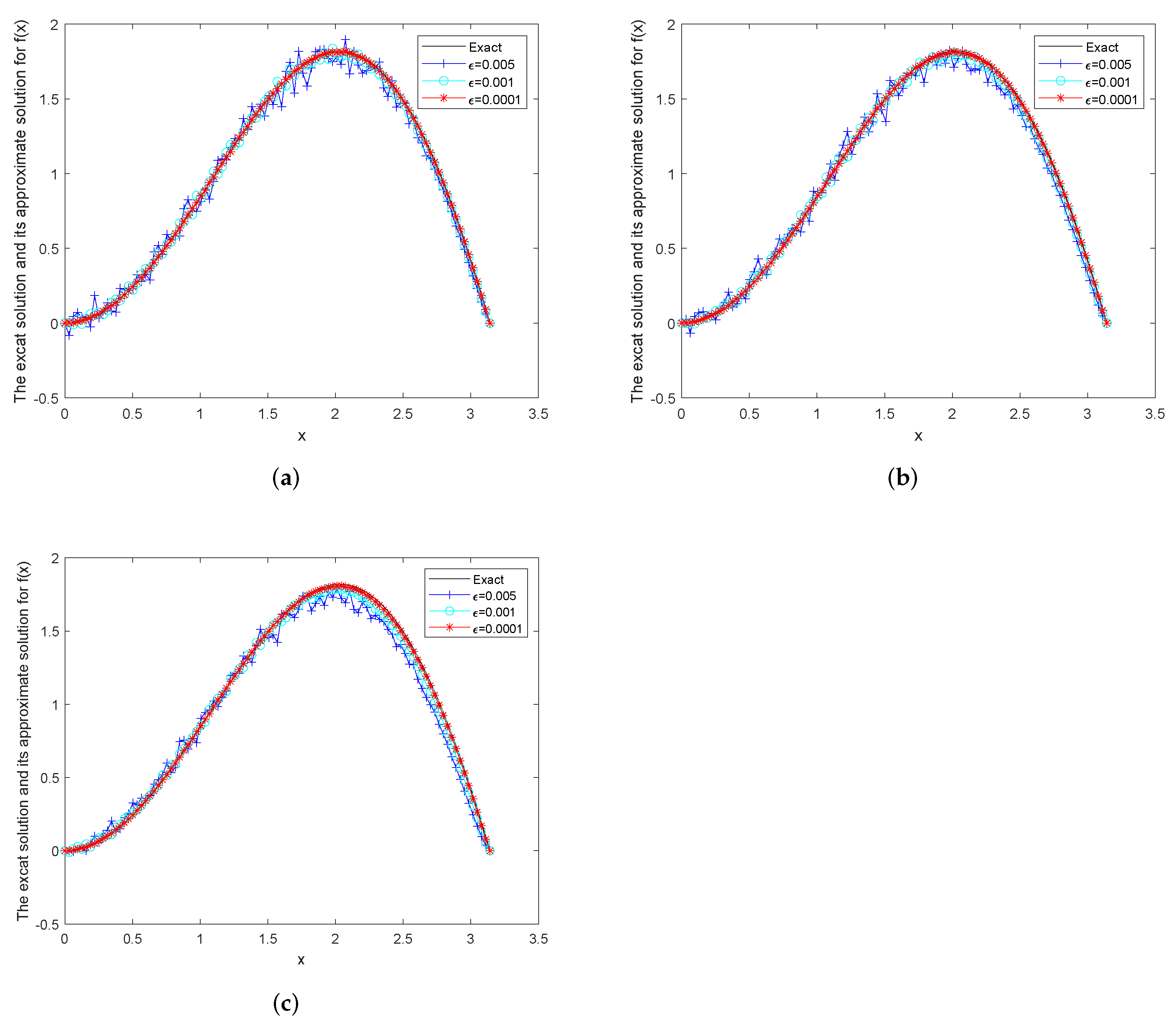
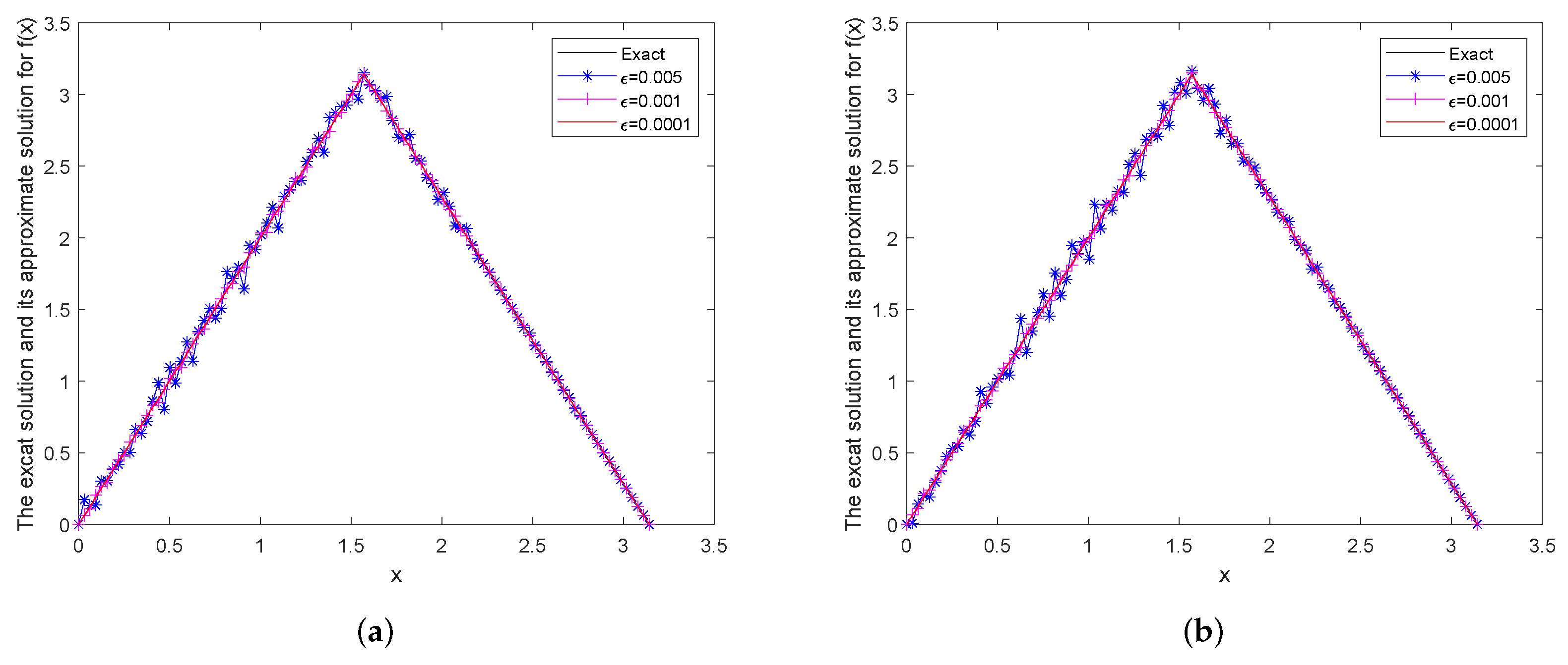
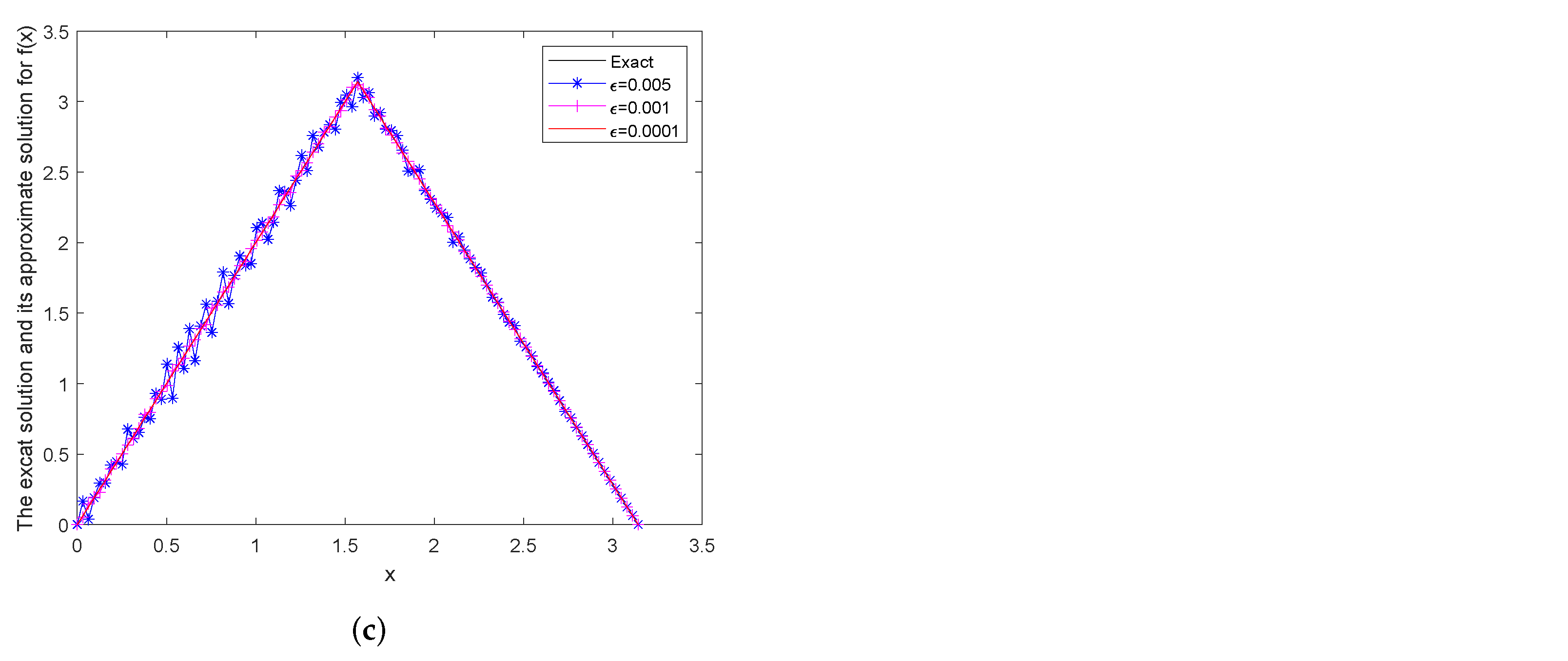
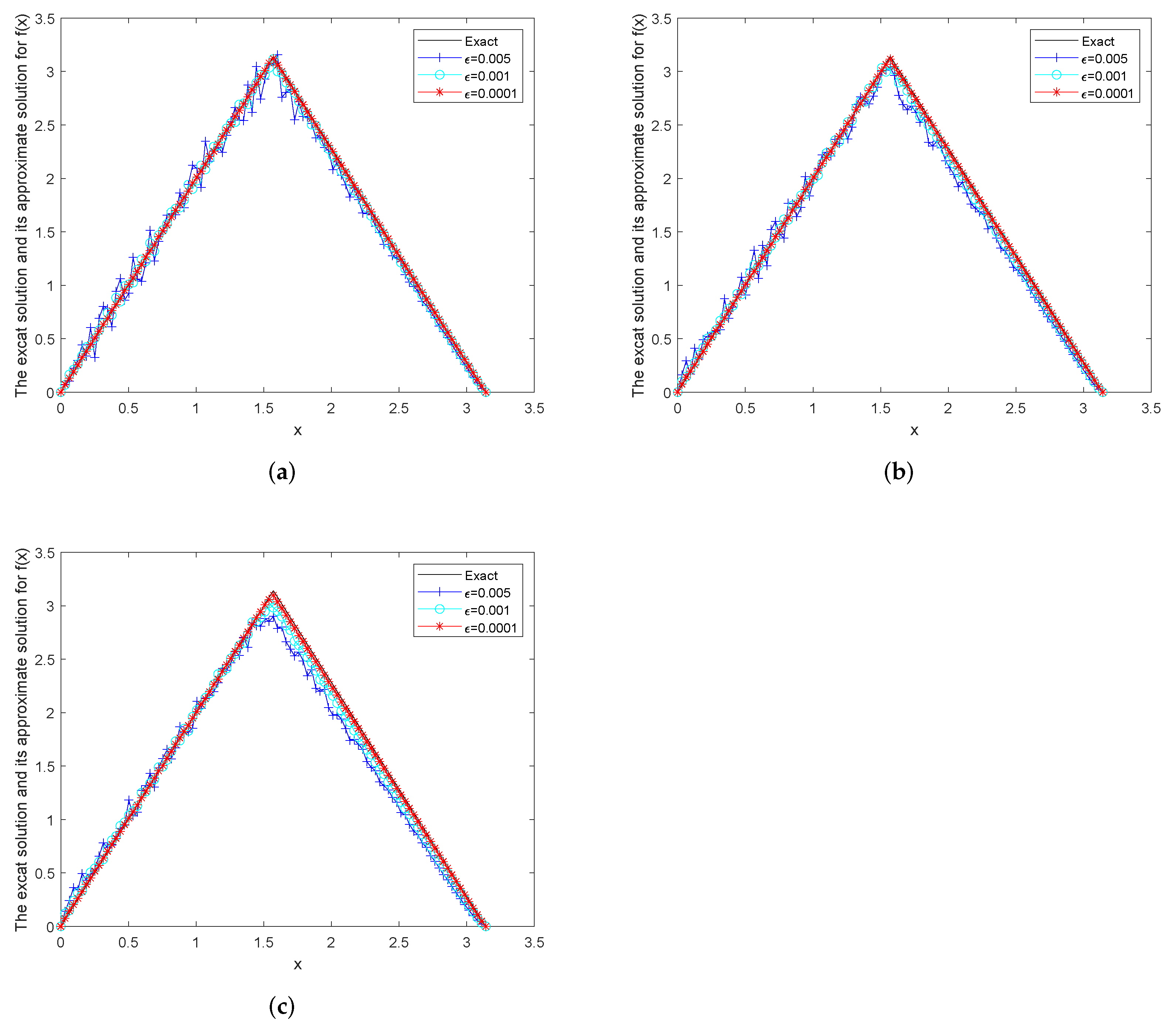
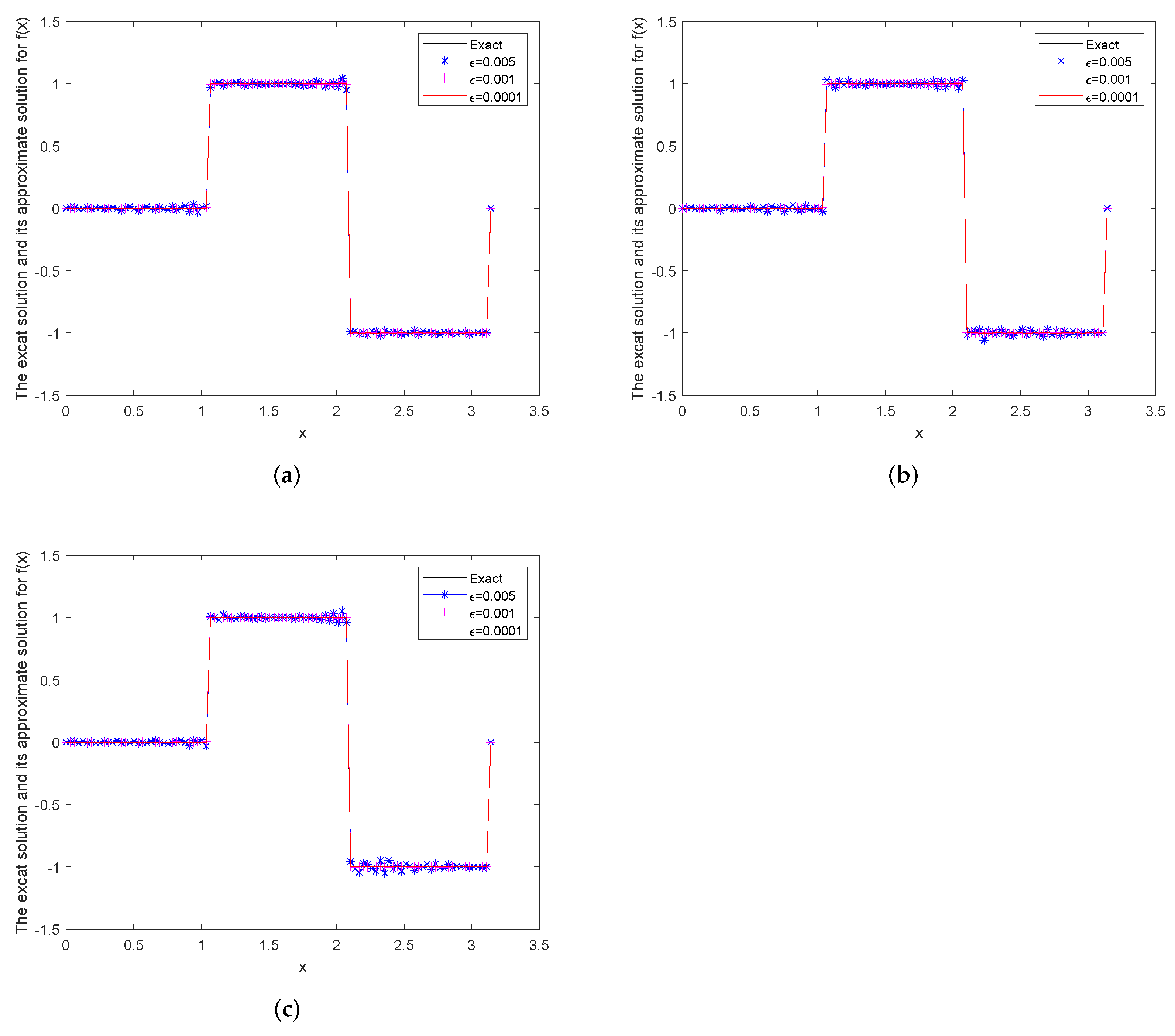
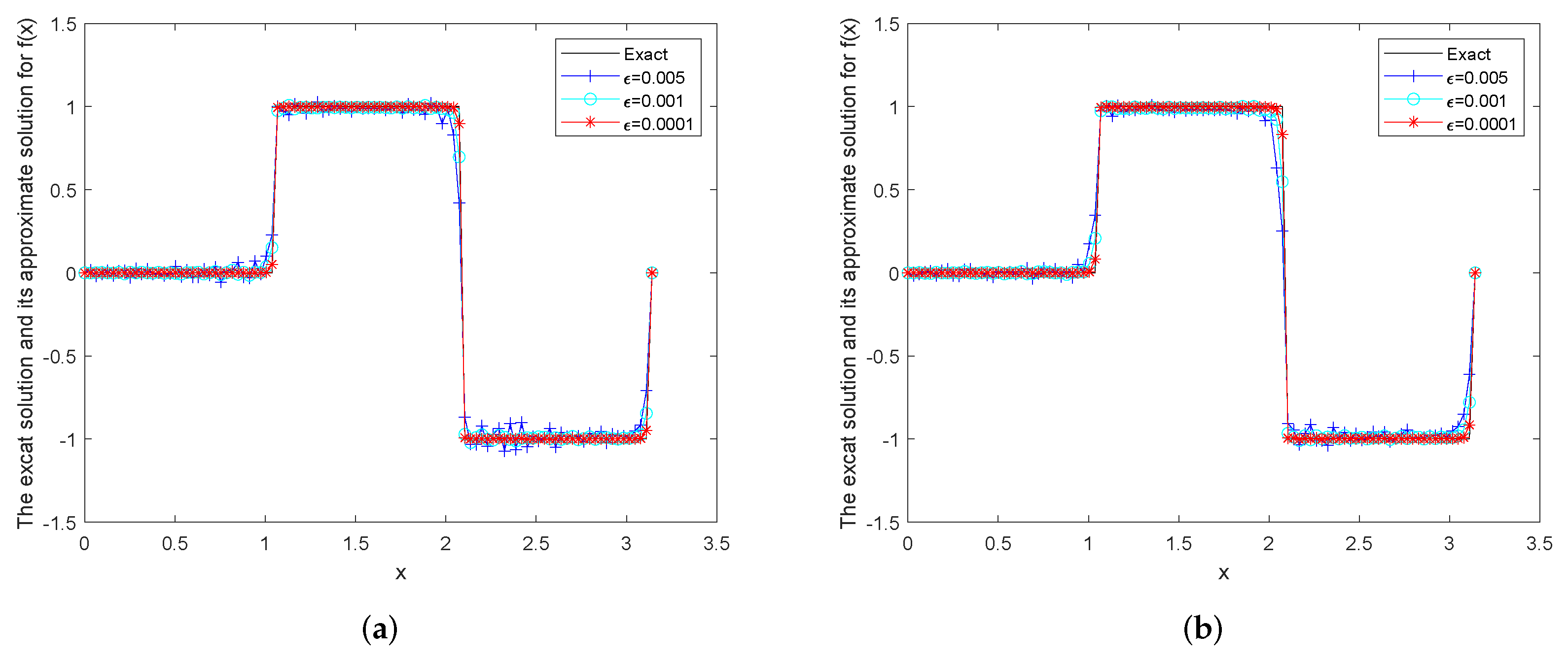
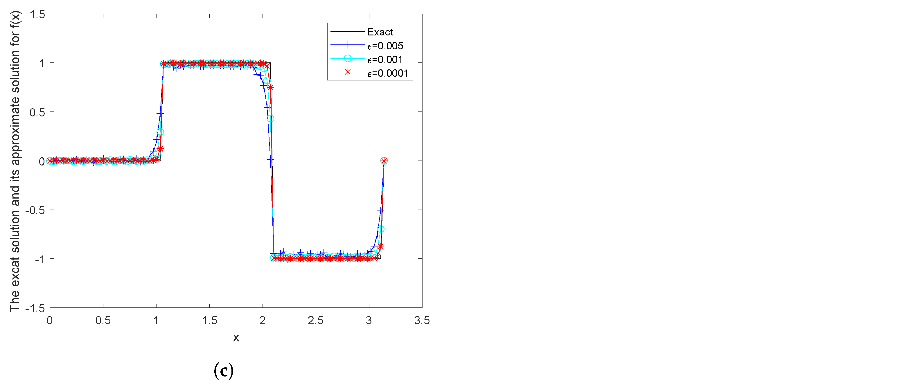
Example 1.

Consider the smooth function

$$f\left(x\right)=xsin\left(x\right),x\in [0,\pi ].$$

Example 2.

Consider the piecewise smooth function

$$f\left(x\right)=\left\{\begin{array}{cc}2x,\hfill & 0\le x\le \frac{\pi }{2},\hfill \\ 2\pi -2x,\hfill & \frac{\pi }{2}\le x\le \pi .\hfill \end{array}\right.$$

Example 3.

Consider the piecewise function

$$f\left(x\right)=\left\{\begin{array}{cc}0,\hfill & 0\le x\le \frac{\pi }{3},\hfill \\ 1,\hfill & \frac{\pi }{3}\le x\le \frac{2\pi }{3},\hfill \\ -1,\hfill & \frac{2\pi }{3}\le x\le \pi .\hfill \end{array}\right.$$

Figure 1 shows the exact $f\left(x\right)$ and its Tikhonov regularization approximation solution $f_{\mu }^{\delta }\left(x\right)$ for Example 1 in the case of $\alpha =1.3,1.5,1.7$. Figure 2 shows the exact $f\left(x\right)$ and its Quasi-boundary regularization approximation solution $f_{\eta }^{\delta }\left(x\right)$ for Example 1 in the case of $\alpha =1.3,1.5,1.7$. From Table 1, we find that the smaller $\alpha$ and $\epsilon$, the smaller the relative error between the exact solution and the regularization solution. Figure 3 shows the exact $f\left(x\right)$ and its Tikhonov regularization approximation solution $f_{\mu }^{\delta }\left(x\right)$ for Example 2 in the case of $\alpha =1.3,1.5,1.7$. Figure 4 shows the exact $f\left(x\right)$ and its Quasi-boundary regularization approximation solution $f_{\eta }^{\delta }\left(x\right)$ for Example 2 in the case of $\alpha =1.3,1.5,1.7$. From Table 2, we find that the smaller $\alpha$ and $\epsilon$, the smaller the relative error between the exact solution and the regularization solution. Figure 5 shows the exact $f\left(x\right)$ and its Tikhonov regularization approximation solution $f_{\mu }^{\delta }\left(x\right)$ for Example 3 in the case of $\alpha =1.3,1.5,1.7$. Figure 6 shows the exact $f\left(x\right)$ and its Quasi-boundary regularization approximation solution $f_{\eta }^{\delta }\left(x\right)$ for Example 3 in the case of $\alpha =1.3,1.5,1.7$. From Table 3, we find that the smaller $\alpha$ and $\epsilon$, the smaller the relative error between the exact solution and the the regularization solution.

Figure 1. The comparison of the exact solution $f\left(x\right)$ and its Tikhonov regularization approximation solution $f_{\mu }^{\delta }\left(x\right)$ of Example 1 with $\alpha =1.3,1.5,1.7$ for $\epsilon =0.005,0.001,0.0001.$ (a) Comparison between exact solution and regularization solution when $\alpha =1.3$. (b) Comparison between exact solution and regularization solution when $\alpha =1.5$. (c) Comparison between exact solution and regularization solution when $\alpha =1.7$.

Figure 2. The comparison of the exact solution $f\left(x\right)$ and its Quasi-boundary regularization approximation solution $f_{\eta }^{\delta }\left(x\right)$ of Example 1 with $\alpha =1.3,1.5,1.7$ for $\epsilon =0.005,0.001,0.0001.$ (a) Comparison between exact solution and regularization solution when $\alpha =1.3$. (b) Comparison between exact solution and regularization solution when $\alpha =1.5$. (c) Comparison between exact solution and regularization solution when $\alpha =1.7$.

Table 1. The relative errors between the exact solution and the regularization solutions of Example 1 with different $\alpha$.

$\mathit{\epsilon }$		0.005	0.001	0.0001
$\alpha =1.3$	Tikhonov	0.0299	0.0058	0.0007
	Quasi-boundary	0.3749	0.1361	0.0300
$\alpha =1.5$	Tikhonov	0.0319	0.0072	0.0007
	Quasi-boundary	0.4090	0.1724	0.0464
$\alpha =1.7$	Tikhonov	0.0346	0.0063	0.0007
	Quasi-boundary	0.5099	0.2302	0.0722

Figure 3. The comparison of the exact solution $f\left(x\right)$ and its Tikhonov regularization approximation solution $f_{\mu }^{\delta }\left(x\right)$ of Example 2 with $\alpha =1.3,1.5,1.7$ for $\epsilon =0.005,0.001,0.0001.$ (a) Comparison between exact solution and regularization solution when $\alpha =1.3$. (b) Comparison between exact solution and regularization solution when $\alpha =1.5$. (c) Comparison between exact solution and regularization solution when $\alpha =1.7$.

Figure 4. The comparison of the exact solution $f\left(x\right)$ and its Quasi-boundary regularization approximation solution $f_{\eta }^{\delta }\left(x\right)$ of Example 2 with $\alpha =1.3,1.5,1.7$ for $\epsilon =0.005,0.001,0.0001.$ (a) Comparison between exact solution and regularization solution when $\alpha =1.3$. (b) Comparison between exact solution and regularization solution when $\alpha =1.5$. (c) Comparison between exact solution and regularization solution when $\alpha =1.7$.

Table 2. The relative errors between the exact solution and the regularization solutions of Example 2 with different $\alpha$.

$\mathit{\epsilon }$		0.005	0.001	0.0001
$\alpha =1.3$	Tikhonov	0.0285	0.0070	0.0007
	Quasi-boundary	0.6174	0.2137	0.0555
$\alpha =1.5$	Tikhonov	0.0319	0.0056	0.0008
	Quasi-boundary	0.6796	0.2846	0.0882
$\alpha =1.7$	Tikhonov	0.0352	0.0063	0.0006
	Quasi-boundary	0.8650	0.4228	0.1263

Figure 5. The comparison of the exact solution $f\left(x\right)$ and its Tikhonov regularization approximation solution $f_{\mu }^{\delta }\left(x\right)$ of Example 3 with $\alpha =1.3,1.5,1.7$ for $\epsilon =0.005,0.001,0.0001.$ (a) Comparison between exact solution and regularization solution when $\alpha =1.3$. (b) Comparison between exact solution and regularization solution when $\alpha =1.5$. (c) Comparison between exact solution and regularization solution when $\alpha =1.7$.

Figure 6. The comparison of the exact solution $f\left(x\right)$ and its Quasi-boundary regularization approximation solution $f_{\eta }^{\delta }\left(x\right)$ of Example 3 with $\alpha =1.3,1.5,1.7$ for $\epsilon =0.005,0.001,0.0001.$ (a) Comparison between exact solution and regularization solution when $\alpha =1.3$. (b) Comparison between exact solution and regularization solution when $\alpha =1.5$. (c) Comparison between exact solution and regularization solution when $\alpha =1.7$.

Table 3. The relative errors between the exact solution and the regularization solutions of Example 3 with different $\alpha$.

$\mathit{\epsilon }$		0.005	0.001	0.0001
$\alpha =1.3$	Tikhonov	0.0160	0.0039	0.0003
	Quasi-boundary	0.4545	0.2183	0.0725
$\alpha =1.5$	Tikhonov	0.0189	0.0038	0.0003
	Quasi-boundary	0.5941	0.3183	0.1178
$\alpha =1.7$	Tikhonov	0.0222	0.0030	0.0004
	Quasi-boundary	0.7906	0.4252	0.1761

Through the above examples containing different types of functions, we find that the smaller the $\alpha$ and $\epsilon$, the better the approximation between the exact solution and the regularization solution. Both the Tikhonov regularization method and the Quasi-boundary regularization method are effective. Moreover, it can be seen that the fitting effect of the Tikhonov regularization method is better than that of the Quasi-boundary regularization method.

7. Conclusions

This paper focuses on solving an inverse problem related to identifying the spatial source term in a space-time fractional diffusion-wave equation. This problem is known to be ill-posed, as even a small perturbation in the final data can lead to a significant change in the source term. The Tikhonov regularization method and the Quasi-boundary regularization method are employed to address this issue. We apply an a priori bound assumption and priori and posteriori regularization parameter selection rules to derive convergence error estimates for the source term in each case. Finally, we assess the validity, stability, and advantages of both the Tikhonov regularization method and the Quasi-boundary regularization method through numerical experiments involving three types of functions: smooth, piecewise smooth, and non-smooth.