Abstract
Gaussian mixture models are widely employed in serological data analysis to discern between seropositive and seronegative individuals. However, serological populations often exhibit significant skewness, making symmetric distributions like Normal or Student-t distributions unreliable. In this study, we propose finite mixture models based on Skew-Normal and Skew-t distributions for serological data analysis. Although these distributions are well established in the literature, their application to serological data needs further exploration, with emphasis on the determination of the threshold that distinguishes seronegative from seropositive populations. Our previous work proposed three methods to estimate the cutoff point when the true serological status is unknown. This paper aims to compare the three cutoff techniques in terms of their reliability to estimate the true threshold value. To attain this goal, we conducted a Monte Carlo simulation study. The proposed cutoff points were also applied to an antibody dataset against four SARS-CoV-2 virus antigens where the true serological status is known. For this real dataset, we also compared the performance of our estimated cutoff points with the ROC curve method, commonly used in situations where the true serological status is known.
Keywords:
finite mixture models; skew-normal distribution; skew-t distribution; cutoff point; serology MSC:
62P10; 62F99; 62H30; 65C05
1. Introduction
Mixture models allow one to describe the distribution of a random variable as a mixture of various distributions. For a long time, mixture models have captured the attention of researchers primarily due to their flexibility in describing data from a non-homogeneous population, as they can reveal latent subgroups within the overall population. Hence, the heterogeneity comes from the situation where one knows (or suspects) that the observations arise from distinct subpopulations, but no mechanism accurately distinguishes between these subpopulations [1]. This makes the finite mixture models a very important tool to handle special features of the density functions under consideration, such as multimodality, skewness, and heavy tails [1].
Nowadays, finite mixture models have experienced significant breakthroughs and are employed in various domains of science, from medicine and biology to social and actuarial sciences, among others. The widespread use of this approach can be attributed to the versatility of finite mixture models, allowing them to effectively tackle diverse challenges in statistical modeling, including classification, clustering, density estimation, and pattern recognition problems [2]. To provide one relevant example, model-based clustering relies on mixture models, and it is considered a classical and powerful approach to address the unsupervised learning problem of accurately grouping observations into clusters [3]. One of the most recent improvements in this field was made by Melnykov and Wang [4], who addressed the matter of the lack of parsimony when studying clustering analysis in the mixture modeling framework. In the last few years, mixture models have also been extended to network data through stochastic blockmodels, opening a new avenue of extensions and novel models for future research (see [5]).
Serology is a branch of medicine that classically studies proteins, encompassing mainly antibodies found in blood and secretions such as saliva [6]. In this work, we focus on serological data, mainly from serological tests: blood tests that evaluate the presence of a specific antibody in the blood against a particular pathogen. Therefore, serological data can be described as a mixture of serological status distributions: seronegative (antibody-negative) or seropositive (antibody-positive) populations.
An individual is seropositive to a pathogen if they have detectable antibodies specific to that pathogen due to a previous infection or vaccination. However, individuals who have never been infected (or vaccinated) with the pathogen under consideration might have non-zero antibody responses due to cross-reactivity with other pathogens or background noise [7]. The detection of antibodies in the serum samples is classically conducted via enzyme-linked immunosorbent assays (ELISA), where the resulting data are light intensities, also called optical density, which reflects the underlying antibody concentration in the samples [8]. The analysis of serological data proceeds by dichotomizing the amount of antibodies in an individual’s serum using a predefined cutoff point in the antibody probability density function. This procedure allows the classification of individuals into the seronegative (with antibody levels below the cutoff point) or seropositive (with antibody levels above the cutoff point) category [7].
Different criteria for seropositivity determination (which means choosing distinct cutoff points) have a direct impact on the sensitivity and specificity of the respective serological classification [9]. In addition, it might also impact the estimation of the seroprevalence [10] and the following (epidemiological) decision that can be taken when facing a given estimate of this epidemiological parameter. This aspect means that when determining the cutoff point for a serological test, one should consider the benefit of the test, the economic and social consequences of serological misclassification, and the prevalence of the disease in the population. Unfortunately, it turns out that these aspects are often ignored in practice [11].
Considering the serological assays, one of the traditional methods to establish the cutoff point is to consider the logarithmic transformation of the antibody concentration of a known seronegative population and proceed to calculate the mean plus two or three standard deviations [11,12,13,14]. This method is adequate when the antibody distribution of the seronegative population is normally distributed [14]. However, previous studies of different serological data [8] showed evidence against the normality assumption for the antibody levels associated with a putative seronegative population. It has been demonstrated that the antibody concentration of a known seronegative (or seropositive) population is highly skewed [8,15,16], which invalidates the use of the Normal distribution in this context.
Recent literature has shown that a mixture of skewed distributions accurately models serological data, such as Skew-Normal or Skew-t distributions [8,16], as far as these distributions can accommodate the skewness structure of the underlying distribution of the antibody concentration.
Our previous work used three methods based on mixtures of Skew-Normal or Skew-t distributions to empirically determine the seropositivity cutoff points [8]. In this paper, we will analyze the performance of the above methods through simulation studies. Additionally, we will apply these methods to the freely available serological data concerning the SARS-CoV-2 virus [7]. In this dataset, there is information about the actual infection status of the individuals, which takes a relevant role in evaluating the accuracy of the methods developed by [8] to establish the cutoff points. Therefore, we will compare the performance of the above techniques with ROC curve-based methods, which are commonly used to determine the cutoff point for defining seropositivity when the true infection (or disease) status is known [17,18,19,20,21,22,23].
2. Modeling Antibody Data: Skew-Normal and Skew-t Distributions
Serological data can be viewed as arising from two or more latent populations; each population is assumed to represent different levels of exposure to a given antigen. For simplicity, individuals who were never exposed or exposed a long time ago to an infectious agent are considered seronegative. In contrast, individuals exposed to the same infectious agent are considered seropositive. In this scenario, the antibody distribution can be described by a mixture of two or more probability distributions [16]. However, the true serological state of an individual is unknown; therefore, it needs to be estimated.
In many serological studies, it is usual to assume a Normal distribution for the basis of the mixture models. However, the behaviour of antibody distribution is not constant over time, and their concentration decreases after infection [7]. This fact makes the distribution of the seropositive population skewed to the left [24]. To accommodate the possible skewness in the seropositive population, we use the scale mixture of the Skew-Normal (SMSN) class of distributions that include the Skew-Normal and the Skew-t distributions, which will be the focus of our study. A brief description of these distributions is presented below.
2.1. Skew-Normal Distribution
Let a random variable (r.v.) with a Skew-Normal distribution. In this distribution, the parameters , , and can be seen as the location, scale, and shape parameters, respectively. Then the probability density function (pdf) is given by
where ; and is the pdf and the cumulative distribution function of the standard Normal distribution, respectively [8,25,26]. The Skew-Normal distribution is part of a family of distributions called the Scale Mixtures of Skew-Normal distributions (SMSN), of which the Skew-t distribution is also a particular case [8].
2.2. Skew-t Distribution
A random variable W is said to have a Skew-t distribution, , if the pdf is given by
where ; and represents the pdf and the cumulative distribution function of the generalized Student’s t distribution with degrees of freedom, and [8,25,26].
Considering the skewness parameter, , when , the reduces to the and the reduces to the non-central Student’s t distribution, respectively. When , the distribution under analysis shows a positive skew whereas the distribution under analysis shows a negative skew (Figure 1). This aspect of heavy tails to the left or right is important as it impacts on the estimation of the cutoff point for defining serological subpopulations.
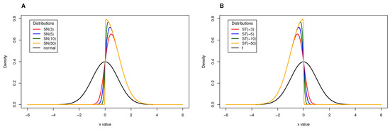
Figure 1.
(A) Skew-Normal distribution considering different values for the skewness parameter showing positive skew. (B) Skew-t distribution considering different values for the skewness parameter showing negative skew.
3. Finite Mixture Models to Describe Serological Data: Estimation of the Parameters
Finite mixture models are very flexible models used to model data from heterogeneous populations, allowing for the capture of population characteristics such as multimodality, skewness, and kurtosis [1]. The rationale behind these types of models is that, given a population, it is possible to consider subpopulations in a finite number, in different proportions, with each subpopulation characterized by a probability density function, with the respective parameter space [27].
In general, let be the partition from a superpopulation G (sample space), and let be the probabilities of sampling an individual belonging to each latent population (with the usual restriction of and . A random variable Z is a finite mixture of independent random variables if the probability density function (pdf) of Z is given by
where is the mixing probability density function (pdf) of associated with the k-th latent population and parameterized by the vector [27].
In the specific case of serological data, let Z be the random variable that represents the antibody level, and let and be the probabilities of sampling a seronegative and a seropositive individual, respectively. Then, the marginal probability density function of Z is given by
where or simply is the mixing probability density function of Z associated with the kth latent population; the latent (unobservable) random variable represents the mixture component for Z, and thus ; is the vector of all unknown parameters of the mixture model, i.e., . In our application is given by the Skew-normal or the Skew-t distributions.
Consider the n-dimensional vector of the observed antibody sample of size n; to estimate the parameters of the model defined by Equation (4), one needs to organize the data to take into account the population from which comes, which is to say the pair , with , where if comes from the second (seropositive) population, or 0 otherwise; , . As a result, one obtains the complete dataset. The complete log-likelihood is thus given by
where is considered a vector of missing values.
Due to the missing structure of the complete dataset from the latent variable, it is crucial to use the EM algorithm to obtain the maximum likelihood estimates for the model’s parameters. The EM algorithm is an iterative method widely used in incomplete data problems where the maximum likelihood estimators (MLE) have no closed expression [28].
In this work, we use the Expectation/Conditional Maximization (ECM) algorithm instead of the classical EM algorithm because mixtures of Skew-Normal or Skew-t distributions lead to a very complex complete-data maximum likelihood estimation [26]. Roughly, the ECM algorithm replaces a complicated M-step of the EM algorithm with several computationally simpler conditional or constrained maximization, or CM steps, each of which maximizes the expected complete-data log-likelihood found in the preceding E-step subject to constraints on the unknown parameters, ; the collection of all constraints is such that the maximization is over the entire space of . Maximizations that take part in the CM-step are over smaller dimensional spaces, which means they are simpler and more reliable than the corresponding full maximization underlying the M-step of the EM algorithm [29,30].
In brief, the sth iteration of the ECM algorithm proceeds as follows:
- E-step:The random variable takes the value 1 if the ith observation belongs to population k, and zero otherwise; thus, , with ; .In this step, one estimates the unobserved component membership, , i.e., the estimated probability that the ith observation comes from the kth population, , given the vector of the antibody levels, , and the current values for the unknown parameters:Afterwards, it estimates the probability of sampling from a seronegative or seropositive population, :
- M-step:In this step, one maximizes the weighted log-likelihood function (derived from Equation (5)), denoted by , with respect to :Therefore,
It should be stressed that the M-step involves the maximization of two weighted likelihoods separately, one for each component under consideration (seropositive and seronegative populations), which reduces the overall complexity of the computations involved in this step.
The process iterates between the E-step and M-step until the difference between two consecutive weighted log-likelihoods is smaller than a prefixed value, which means that convergence has been attained. The ECM algorithm has been proved to share the same appealing convergence properties as the EM [29,30,31].
Considering the SMSN family of distributions, namely the Skew-Normal and the Skew-t distributions, the application of the ECM algorithm in the context of mixtures can be found in [2,26]. The initial values for the parameters are discussed in detail in [26].
To decide which model is the best one among all the models fitted to the same data, we used the Bayesian Information Criterion (BIC) [8].
3.1. Definition of Seropositivity: Methods to Estimate the Cutoff Points in the Mixture Models
Seroprevalence is an epidemiological measure defined by the proportion of seropositive individuals in the sample. For its estimation, it is then necessary to define the serological status of the i-th individual by dichotomising the variable, , which represents the antibody concentration of the individual. This dichotomization is performed by determining a value c such that for antibody values equal to or greater than c, the individual is classified as seropositive and seronegative otherwise. Thus, let Y be the r.v. representing the number of seropositive individuals in a sample of size n, whereby we have to
where represents the seroprevalence, i.e, and is the indicator variable. Considering that the r.v. representing the antibody levels is modeled by a finite mixture of distributions, the way to estimate the cutoff c from the observed data is nonstandard. To determine this cutoff value, we present three estimation methods below.
- -
- Method 1 (M1): It is based on the 99.9%-quantile associated with the estimated seronegative population. This method is the most popular in sero-epidemiology [32,33]. It is often called the rule because the 99.9%-quantile is given by the mean plus three times the standard deviation of a normally distributed seronegative population;
- -
- Method 2 (M2): It relies on the minimum of the density mixture functions. In the case of two latent populations, the cutoff corresponds to the absolute minimum. For three or more latent populations, the cutoff corresponds to the lowest relative minimum. This point can be calculated using Dekker’s algorithm [34]. It should be noted that the minimum of the mixing function is not expected to coincide with the point of intersection of the probability densities of each subpopulation;
- -
- Method 3 (M3): It imposes a threshold in the so-called conditional classification curves [32]. Under the assumption that all components but the first one referred to seropositive individuals, the conditional classification curve for the i-th individual given the antibody level is defined asIn turn, the classification curve of seronegative individuals is simply given byAfter calculating these curves, one can impose a minimum value for the classification of each individual. In this case, two cutoff values arise in the antibody distribution, one for the seronegative individuals and another for seropositive individuals. Mathematically, the classification rule is given as followswhere and are the cutoff values in the antibody distribution that ensure a minimum classification probability (say 90%). In practice, one can use the bisection method to calculate these cutoff values in practice, providing an initial interval where they might be located [32].
3.2. Software
For this study, we used the R software version 4.2.3. In particular, we used the package mixsmsn to fit different mixture models based on SMSN [35]. To estimate the model parameter via the EM algorithm, we used the function smsn.mix. For fitting the Student’s t-distribution, we considered the R package extraDistr [36]; namely, the function dlst to calculate their density, the function plst to define the cumulative distribution function, and the function rlst to generate random samples in the simulation study. The fitting of the Skew-Normal distributions was performed with the package sn [37]. The functions dsn, psn, and rsn were used to calculate the probability density function, the cumulative distribution function, and generate random samples of the Skew-Normal distribution, respectively. In the case of the Skew-t distribution, the functions dst, pst, and rst were used to calculate the probability density function, the cumulative distribution function, and generate random samples, respectively.
4. Simulation Study
We used Monte Carlo simulation to assess the performance of the cutoff points techniques (see Section 3.1). We based our analyses on the usual mixture distributions used in serological data (Normal and Student-t distributions) and their skewed versions proposed in this article. Overall, we want to check whether the performance of the proposed techniques is worse in symmetrical distributions (usually considered when analysing this type of data). Then, four simulation scenarios regarding the mixture models were considered (Table 1).

Table 1.
Simulation scenarios and theoretical parameter values for seronegative and seropositive populations.
Another goal of the simulation was to evaluate how well the fitted mixture models can distinguish between the two populations under study, seropositive or seronegative. Accordingly, we considered different proportions of seropositive (and consequently seronegative) individuals in the dataset. That is, varying the weights assigned to the populations in the mixture model allowed us to check the ability of the model to identify the seropositive component even when the weight assigned to that component was low. The practical implications of varying the weight of the seronegative and seropositive population is identifying false negative and false positive individuals. In addition, when the proportion of seronegative individuals is very high relative to seropositive individuals, more effective decisions can be made to control the number of infections in the population. On the other hand, the opposite scenario is essential for the effectiveness of vaccination in the population, particularly for individuals who may have lost immunity.
To proceed with the simulation study, we randomly selected an antigen from the practical case presented in Section 5 and fitted a mixture of Normals, Skew-normal, Student-t and Skew-t distributions to this data. The parameter estimates of each fitted model were considered the true parameters for the simulation study (Table 1). To assess the impact of sample size and the percentage of seronegative (or seropositive) individuals in the mixture model on the performance of the methods in identifying the threshold value for distinguishing seronegative from seropositive individuals, we considered sample sizes (n) between 50 and 500, with fixed intervals of 50. We set for the probability of a seronegative individual in the mixture model. In each simulation scenario, replicate samples were drawn. For each simulated sample, the parameters of the two-component mixture model were estimated by maximum likelihood (via the ECM algorithm described in Section 3).
The primary goal of the simulation study is to assess the differences between the cutoff values obtained by the three methods under study and the true cutoff points. Therefore, the evaluation criteria must focus on quantifying these differences. The two-component mixture models defining various simulation scenarios vary based on the weights assigned to the seropositive/seronegative components and the underlying probability distribution. Consequently, the true cutoff values also vary according to the scenario under consideration. Table 2 provide the true cutoff values for each situation considered in the simulation study.
Table 2.
Simulation study: Theoretical cutoff values considered for each method by mixture distribution and seronegative weight.
Next, we report the following performance measures for the three methods under consideration: relative bias (RB) and mean squared error (MSE). Let be the estimated cutoff point based on the i-th simulated sample () and for the jth method (, representing methods M1, M2, and M3, respectively); is the theoretical cutoff point based on the jth method. Then, the Relative Bias (RB) and the estimated Mean Squared Error (MSE) for the jth method based on replicate samples are given by:
where , the average of the cutoff points obtained from the jth method, for all simulations performed.
We also compute a distribution-free approximate confidence interval for each cutoff value derived from the three methods under study using the empirical percentiles method, , where is the empirical cumulative distribution function of the cutoff points’ sample, , with N representing the number of replicates.
Next, we outline the algorithm of the simulation procedure used in this article.
Simulation Procedure
Let Z be the random variable representing the antibody level, which is described by a two-component mixture model with probability density function given by expression (4). The mixture probability density functions analyzed here are the Normal, Skew-normal, Student-t, and Skew-t distributions.
For each combination of two-component mixture distribution with fixed weight from the set (and thus ) and the theoretical vector of parameters given by Table 1, we proceed as follows:
- 1
- For to N (run N Monte Carlo simulations)
- S.1
- Simulate a sample with dimension n of antibodies concentration:
- Generate seronegative individuals using .
- The remaining individuals from the sample with dimension n are seropositive.
- Based on the theoretical model under consideration, generate a random sample of antibody concentration, with the sample size equal to n: the m observations of 1(S.1)i are drawn from the seronegative population, whereas the observations of 1(S.1)ii come from the seropositive population.
- S.2
- Fit a two-component mixture model to the simulated sample using the ECM algorithm described in Section 3.
- S.3
- Estimate the cutoff points based on the three methods under study, , where i denotes the ith simulated sample, represents the method under consideration, M1, M2, and M3, respectively.
- 2
- Store the estimated cutoff values in a matrix, , where the jth column contains the cutoff points’ sample with dimension N, for the jth method (), i.e., the N-dimensional column vector , and .
- 3
- Calculate the RB and the estimated MSE according to (9) for each cutoff points’ sample stored in the N-dimensional column vector
- 4
- Determine the empirical cumulative distribution function from the N-dimensional column vector , of the estimated cutoff points; then, construct a distribution-free approximate confidence interval for the true cutoff point from method , based on the percentile method [38].
The main results from the simulation study are provided in Figure 2, Figure 3, Figure 4, Figure 5, Figure 6 and Figure 7 and Appendix C Table A3, Table A4, Table A5, and Table A6. We start by analyzing the bias properties. Considering the balanced scenario (), we observe that, for both the mixture of Normal distributions and the respective skewed variant (Figure 3A,B), the cutoff estimates exhibit moderate positive bias across all considered methods. Additionally, there is a stabilizing pattern in bias behavior, indicating that the bias remains almost constant as the sample size increases. However, the cutoff derived from the M1 method is the one that shows the worst behavior in the framework of the mixture of Normal distributions. Concerning the mixture of Student-t distributions (Figure 3C,D), the M1 method has a large positive bias, stabilizing at . Methods M2 and M3 demonstrate comparable performances, displaying a generally unbiased pattern. Finally, the mixture of Skew-t distributions unfolds an erratic behavior of the M1 method, exhibiting an initial positive bias for and decreasing to negative biases as the sample size increases. Cutoff estimates linked to methods M2 and M3 consistently display stable moderate negative bias patterns.
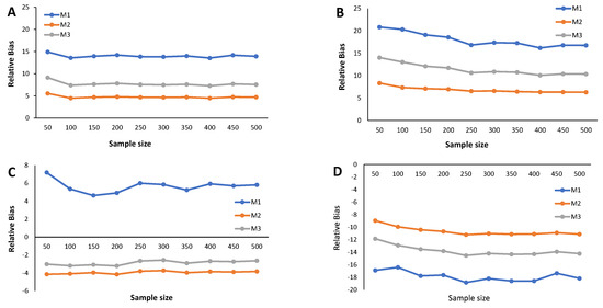
Figure 2.
Results from the simulation study: Relative bias of the cutoff points for methods M1, M2, and M3 considering ; sample sizes vary between and 500, with intervals of 50. (A) Mixture of Normal distributions. (B) Mixture of Skew-Normal distribution. (C) Mixture of Student-t distribution. (D) Mixture of Skew-t distribution.
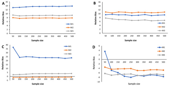
Figure 3.
Results from the simulation study: Relative bias of the cutoff points for methods M1, M2, and M3 considering ; sample sizes vary between and 500, with intervals of 50. (A) Mixture of Normal distributions. (B) Mixture of Skew-Normal distribution. (C) Mixture of Student-t distribution. (D) Mixture of Skew-t distribution.
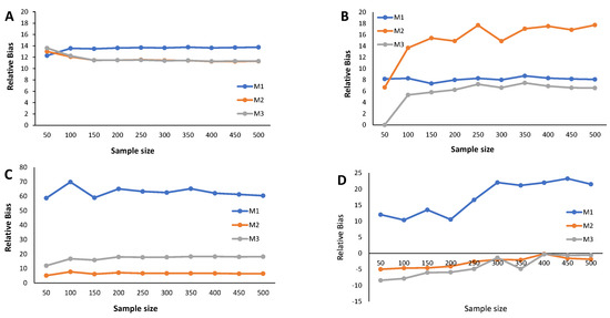
Figure 4.
Results from the simulation study: Relative bias of the cutoff points for methods M1, M2, and M3 considering ; sample sizes vary between and 500, with intervals of 50. (A) Mixture of Normal distributions. (B) Mixture of Skew-Normal distribution. (C) Mixture of Student-t distribution. (D) Mixture of Skew-t distribution.
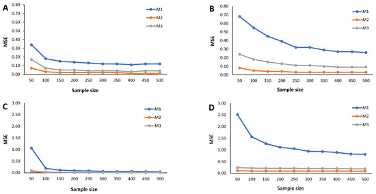
Figure 5.
Results from the simulation study: Estimated MSE of the cutoff points for methods M1, M2, and M3 considering ; sample sizes vary between and 500, with intervals of 50. (A) Mixture of Normal distributions. (B) Mixture of Skew-Normal distribution. (C) Mixture of Student-t distribution. (D) Mixture of Skew-t distribution.
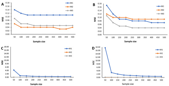
Figure 6.
Results from the simulation study: Estimated MSE of the cutoff points for methods M1, M2, and M3 considering ; sample sizes vary between and 500, with intervals of 50. (A) Mixture of Normal distributions. (B) Mixture of Skew-Normal distribution. (C) Mixture of Student-t distribution. (D) Mixture of Skew-t distribution.
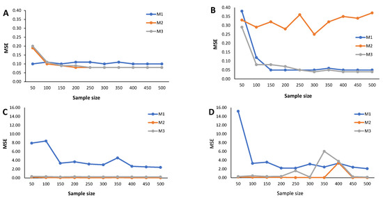
Figure 7.
Results from the simulation study: Estimated MSE of the cutoff points for methods M1, M2, and M3 considering ; sample sizes vary between and 500, with intervals of 50. (A) Mixture of Normal distributions. (B) Mixture of Skew-Normal distribution. (C) Mixture of Student-t distribution. (D) Mixture of Skew-t distribution.
When (indicating a predominant population of seropositive individuals, ), the cutoff estimates based on method M1 exhibit the poorest performance (Figure 2), although its behavior remains stable as the sample size increases. The cutoff estimates from the other two methods share this regular pattern as the sample size increases. Moreover, cutoff estimates derived from M2 and M3 demonstrate similar performance, displaying a moderate positive bias for the mixture of normals and Skew Normals and a moderate negative bias within the context of the mixture of Student-t and the mixture of Skew Student-t distributions, emphasizing the bias for the latter case.
Figure 4 illustrates the relative bias of the cutoff estimates obtained from methods M1, M2, and M3 when , reflecting a scenario where only of the population is seropositive, indicating high susceptibility to the considered virus. For the mixture of Normals, all three methods yield cutoff estimates with similar performance in terms of bias, displaying moderate positive bias (Figure 4A). Surprisingly, Figure 4B reveals an unexpected behavior in the cutoff estimates from the M2 method, exhibiting fluctuations as the sample size increases and showing a larger relative bias than its competitors. This characteristic might be linked to the method’s incapacity to precisely model a mixture of Normal distributions, particularly in cases where one of the components has a very small weight in the mixture. Methods M1 and M2 produce cutoff estimates with stable patterns. For the mixture of Student-t and the mixture of Skew-t distributions (Figure 4C,D), cutoff estimates from methods M2 and M3 exhibit good performance, showing small positive biases in the former and small negative biases in the latter. Conversely, method M1 generates cutoff estimates with large and erratic biases.
The estimated MSE (Figure 5, Figure 6 and Figure 7) measures the accuracy of the cutoff points’ estimates. To avoid misinterpretations, we must start by stressing that the ranges of the y-axes for the mixture of Normals (symmetrical and skewed versions) are significantly narrower than for the mixture of Student-t distributions (symmetrical and skewed versions). An overview of the variability in the cutoff estimates reveals that the M1 method consistently emerges as one that produces the cutoffs with the least performance, irrespective of the probability of seropositivity in the underlying population, for medium sample size. With increasing sample size, the cutoff values based on the M1 method rapidly converge to values near zero, indicating a significant reduction in estimate variability. Cutoff values derived from the M2 and M3 methods reveal a good convergence to values near zero as the sample grows. These characteristics hold for the different values of , that is, the weight of the seronegatives in the mixture. A word of caution should be noted regarding the cutoff estimates based on the M2 method for in the case of the Skew Normal distribution (Figure 7B) as it exhibits a seemingly increasing MSE as the sample size grows. This misleading impression might be due to the scale of the y-axis, which has a range of values very close to zero. Nevertheless, a similar pattern appeared when analyzing the corresponding relative bias (Figure 4B).
5. Applications to SARS-CoV-2 Real Data
We analysed IgG antibody responses against four SARS-CoV-2 spike or nucleoprotein antigens: RBD—glycoprotein receptor-binding domain; —S trimeric spike protein; S1—spike glycoprotein S1 domain; S2—SARS-CoV-2 spike glycoprotein S2 domain. Antibodies were measured in serum samples collected up to 39 days after symptom onset from 215 adults in four French hospitals (53 patients and 162 healthcare workers) with quantitative RT-PCR-confirmed SARS-CoV-2 infection. Three hundred and thirty-five negative control serum samples were collected from France, Thailand, and Peru before the COVID-19 pandemic [7]. A detailed description of lab procedures can be found in the original study [7].
SARS-CoV-2 infection, which causes the devastating and often lethal COVID-19 disease, was first detected in the Chinese province of Wuhan in December 2019 [7]. Rapidly, SARS-CoV-2 infection spread worldwide, and the COVID-19 disease was declared a pandemic by the World Health Organization.
The detection of the virus is so far achieved by the so-called reverse quantitative PCR reverse transcriptase (RT-qPCR) on samples from nasopharyngeal or throat swabs [7]. However, in general, only symptomatic individuals or people in close contact with detected cases are tested, which might lead to overestimating the proportion of individuals infected with SARS-CoV-2 [39]. Alternatively, serological testing allows for detecting asymptomatic individuals exposed to the infection. In addition, serological testing can quantify the degree of exposure to the infection in the population. In this context, it is crucial to estimate seroprevalence at the population level, i.e., the proportion of seropositive individuals that show antibodies against any SARS-CoV-2 antigen [40].
5.1. Patients’ Characteristics
For this study, data relating to 549 individuals were analysed. Serum samples were collected from individuals with confirmed SARS-CoV-2 infection by PCR test in four hospital units from Paris, namely: 4 (0.7%) from the Hôpital Bichat, 49 (9.0%) from the Hôpital Cochin, and 161 (29.3%) from the Nouvel Hôpital (Strasbourg). Regarding the negative controls, 68 (12.4%) are from the Thai Red Cross (TRC), 90 (16.4%) from Peruvian donors (NHP), and 177 (32.2%) from the France blood donors (Établissement Français du Sang). For each antigen under analysis, the logarithmic transformation base ten was considered for the concentration of antibodies against that antigen.
Regarding the analysis of antibodies by the individuals who performed PCR test, there were statistically significant differences between individuals who tested negative and positive for SARS-CoV-2 by Mann-Whitney test (RBD: 1.64 versus 3.48, ; S1: 1.72 versus 2.59, ; S2: 1.79 versus 2.99, ; : 1.59 versus 3.43, ) (Figure 8). Such differences were expected given the general knowledge about the infection status, i.e., individuals who have already been exposed to the virus have a higher concentration of antibodies than those who are still susceptible.
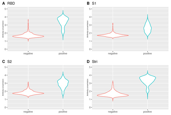
Figure 8.
Violin plot for the antibody concentration by infection status. (A) RBD antigen. (B) S1 antigen. (C) S2 antigen. (D) antigen. Number of negative individuals: 335; the number of positive individuals: 214. The antibody concentration on the y-axis is given in log10 units.
5.2. Mixture Model Approach and Cutoff Points
We fitted the different mixture models analyzed in this paper to the SARS-CoV-2 datasets considering two subpopulations (seronegative and seropositive subpopulations). Specifically, we adjusted two-component mixture models based on the Normal, Skew-normal, t-Student, and Skew-t distributions. Table A1 provides a summary of the main results.
According to the BIC values, the model based on the Skew-Normal distribution was considered the best fit for the following antigens: RBD (BIC = 852.25), S1 (BIC = 561.63), S2 (BIC = 775.29). For the case of the Stri antigen (), the best model was found to be the Skew-t distribution (BIC = 915.82) (Table A1). Table 3 displays the parameter estimates for the optimal mixture models determined by the BIC criterion. Additionally, graphical representations of the estimated densities for each antigen are shown in Figure 9.
Table 3.
Results from fitting two-component mixture model to antibody concentration by antigen: Estimated parameters for the best model based on the BIC criterion.
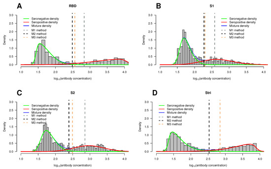
Figure 9.
Histogram of the antibody concentration data by antigen. Overlaid on the histograms are the seropositive estimated density functions (red lines), the seronegative estimated density functions (green lines), and the estimated two-component mixture density (blue lines). The vertical dotted lines correspond to the cutoff points based on methods M1 (gray), M2 (black), and M3 (orange). (A) RBD antigen. (B) S1 antigen. (C) S2 antigen. (D) antigen. The antibody concentration on the x-axis is given in units.
In line with results from previous studies, the seronegative population is skewed to the right, whereas the seropositive population reveals skewness to the left; this feature is not very pronounced in the case of S1 () and S2 () antigens (Table 3).
After identifying the mixture model that best fits each dataset, we categorized the antibody concentration for each antigen by estimating the respective cutoff point. To achieve this goal, we employed the methods M1, M2, and M3 as previously described in Section 3.1. The results are comprehensively detailed in Appendix A Table A1. In addition to the estimated cutoff points, Table A1 also shows a few performance measures, namely sensitivity (sen), specificity (spec), and accuracy (ACC). Graphical representations of the cutoff points for the three methods under consideration are displayed in Figure 9, where these points are indicated by vertical dotted lines.
It is important to emphasize that when adjusting a mixture of Student-t distributions (either symmetric or skewed) for the S antigen, calculating the method’s sensitivity and accuracy based on the M1 method (99.9%-quantile for the seronegative population) was impossible due to the high value assumed by the respective quantile. This characteristic led to the complete absorption of the seropositive population by its seronegative counterpart (Table A1).
Considering the best-fitted models, one can conclude that estimation of the cutoff point based on the minimum densities of the mixture model (M2 method) proved to be the method with the highest sensitivity for classifying seropositive individuals regardless of the antigen under consideration: RBD antigen: cutoff = , sens = ; S1: cutoff = , sens = ; S2: cutoff = , sens = ; S: cutoff = , sens = (Table A1). Method M2 also yields the highest proportion of correct results (accuracy) for the RBD antigen (cutoff = , ACC = ), S1 (cutoff = , ACC = ), and S2 (cutoff = , ACC = ). Regarding the S antigen, both methods M2 and M3 achieve the same accuracy of (Table A1).
Since the true infection status of the individuals is known for this case study and to reinforce the performance of the proposed methods, we computed ROC curve-based methods (hereafter designated as the M4 method) through univariable logistic regression analysis. We considered the disease status as the binary outcome variable and the (antibody concentration) for each antigen as the covariate. The ROC curve is commonly used to evaluate the performance of biomarkers, and the area under the ROC curve (AUC) summarizes this performance. To estimate the optimal cutoff point and consequently the sensitivity and specificity, we used the R package OptimalCutPoints and the method that minimizes the misclassification rate that is well described in [41].
Results from the ROC curve-based methods are presented in Appendix B Table A2, where the estimated cutoff points for each antigen are reported, along with the same performance measures used to evaluate methods M1, M2, and M3, namely sensitivity, specificity, and accuracy. Additionally, we calculated the Area Under the Curve (AUC) and the respective confidence interval. A graphical representation of the main results, facilitating the comparison of methods M1 to M4 in terms of performance measures, is displayed in Figure 10. The source data are stored in Appendix A Table A1 (results from M1 to M3 methods) and Appendix B Table A2 (ROC curve-based method, M4).
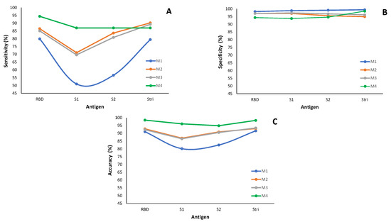
Figure 10.
Classification performance of the methods M1 to M4 by antigen: (A) Sensitivity. (B) Specificity. (C) Accuracy. The measures for methods M1 to M3 are based on the best-fitted model for each antigen and are detailed in Appendix A Table A1; method M4 relies on information in Appendix B Table A2.
Regarding sensitivity, the M1 method performs worse than the others under consideration (Figure 10A, Appendix A Table A1). The worst case occurs for the sensitivity associated with the antigen S1, where approximately fifty percent of infected individuals are misclassified with M1. More precisely, only of infected individuals are correctly classified as seropositive. When considering the antigen S2, the sensitivity shows an increase of percentage points compared to the antigen S1 for method M1; however, both results remain low in terms of sensitivity. Methods M2 and M3 behave similarly in terms of sensitivity for all the antigens in analysis. Method M4 (ROC curve-based method) has the highest true positive rate compared to the remaining three methods under study (Figure 10A and Appendix B Table A2).
In terms of specificity (Figure 10B), all four methods under consideration exhibit similar behavior across all antigens, with specificities above . This feature indicates that the methods accurately identify seronegative individuals in the subpopulation of the non-infected by SARS-CoV-2.
Concerning the accuracy, method M1 exhibits the worst behavior, similar to what happens with sensitivity. However, it is important to note that the accuracy values are higher than sensibility, with a minimum of for the S1 antigen (Figure 10B and Appendix A and Appendix B Table A1 and Table A2 ).
In summary, method M1 exhibits the lowest performance in accurately classifying individuals as seronegative or seropositive. These findings align with the conclusions drawn from the simulation study.
6. Discussion and Conclusions
Serological data can be described as a mixture of serological status distributions: seronegative (antibody-negative) or seropositive (antibody-positive) populations. In this framework, one must thus use a mixture model with two components. Therefore, it is crucial to accurately calculate the threshold that distinguishes between seropositive and seronegative populations.
This study aimed to evaluate the performance of three cutoff point estimation methods developed by [8] for defining the seropositivity of an individual using mixtures of Skew-Normal and Skew-t distributions. The 99.9%-quantile (or 3- rule, if it is assumed to be a Normal distribution) method is commonly used in practice as the gold standard to estimate the cutoff point in serological tests assuming a Normal distribution for the components of the mixtures [11,12,13,14]. This method (M1 method) is compared with two other methods, M2 and M3. Method M2 relies on the minimum of the density function derived from a mixture model with two components, whereas the cutoff point obtained from method M3 is based on conditional classification curves.
A Monte Carlo simulation study was conducted to evaluate the performance of the cutoffs obtained by each method based on the mixture of two Normal or two Student-t distributions or their skewed variants. The relative bias, estimated mean square error, and confidence intervals for the true cutoff values based on the three methods under study were calculated.
When a new virus appears in the population, there is a natural tendency for the proportion of susceptible individuals (seronegative individuals) to be higher than seropositive individuals. This context corresponds to the phase in which early identification of the infected people is essential for pandemic control. However, total control of the spread of the virus only occurs when there is vaccination or eradication of the virus. Due to these complex dynamics, in the simulation study we decided to evaluate the effect of different percentages of seropositive (and obviously, seronegative) individuals in the overall population on the determination of cutoff points as well as the ability of the modeling procedure to correctly capture two components in the mixture model. In addition to evaluating the effect of different analytic expressions to describe the two-component mixture model, the simulation study allowed us to study distinct pandemic evolution scenarios due to varying the probability of seropositivity (or seronegativity) in the population.
For the majority of the two-component mixture models studied in the simulation carried out in this paper, we can experimentally conclude that the traditional method (M1 method) has the poorest performance in terms of bias and estimated MSE when compared with methods M2 and M3. The low performance found in the context of this simulation study can be explained in light of heavy-tailed distributions (such as the Skew normal or Skew-t distributions) to fit serological data. In fact, the calculation of the 99.9%-quantile (3- rule, for the normal distribution) relies only and exclusively upon the population of seronegative individuals. Considering these heavy-tailed distributions are skewed to the right, the seropositive population is absorbed by the 99.9%-quantile from the seronegative population.
For the methods M2 and M3 studied in this work, we found that both are moderately biased and with small variability. As expected, the larger the sample size, the smaller the estimated mean square error of the cutoff points estimates.
Lastly, we used real data regarding SARS-CoV-2 infections to apply these methods and evaluate their performance. Since the true disease status of the individuals was known in advance, we also computed the ROC curve-based method, which is a standard procedure to evaluate the performance of biomarkers. In line with the conclusions from the simulation study, method M1 has been revealed as the one with the lowest performance in identifying the cutoff point to distinguish between a seronegative and seropositive individual. Therefore, methods M2 and M3 are preferable to method M1.
A limitation of this study is that the different mixture models were fitted using the same distribution for the two components. If the components of the mixture model were distinct, this would directly affect the estimated cutoff points and might increase the performance of the methods under consideration. Future research on this topic should be carried out.
In conclusion, we recommend using mixture models based on distributions of the SMSN family to analyze serological data, given the flexibility of these models and the proposed M2 or M3 methods for determining cutoff points. These methods have been proven to be a reliable alternative to the gold standard method based on the 99.9%-quantile (or 3- rule for the Normal distribution).
Author Contributions
Conceptualization, T.D.-D., H.M. and N.S.; methodology, T.D.-D. and N.S.; software, T.D.-D. and H.M.; validation, T.D.-D., H.M. and N.S.; formal analysis, T.D.-D. and H.M.; investigation, T.D.-D., H.M. and N.S. All authors have read and agreed to the published version of the manuscript.
Funding
This research was funded by FCT—Fundação para a Ciência e Tecnologia, Portugal, under the project UIDB/00006/2020. DOI: https://doi.org/10.54499/UIDB/00006/2020.
Data Availability Statement
Data are available upon request.
Conflicts of Interest
The authors declare no conflicts of interest.
Appendix A. Bayesian Information Criteria (BIC), Sensitivity, Specificity, and Accuracy by Method for Each Antigen
Table A1.
BIC values, cutoff value estimates, sensitivity, specificity, and accuracy for each method under study. C denotes the cutoff point estimate.
Table A1.
BIC values, cutoff value estimates, sensitivity, specificity, and accuracy for each method under study. C denotes the cutoff point estimate.
| Method M1 | Method M2 | Method M3 | ||||||||||||
|---|---|---|---|---|---|---|---|---|---|---|---|---|---|---|
| Antigen | Distribution | BIC | C | Sens (%) | Spec (%) | ACC (%) | C | Sens (%) | Spec (%) | ACC (%) | C | Sens (%) | Spec (%) | ACC (%) |
| RBD | Normal | 953.00 | 2.65 | 84.11 | 97.61 | 92.35 | 2.33 | 90.18 | 95.52 | 93.44 | 2.37 | 88.79 | 95.82 | 93.08 |
| Skew-Normal | 852.25 | 2.83 | 79.91 | 98.21 | 91.07 | 2.49 | 86.45 | 97.01 | 92.89 | 2.56 | 85.05 | 97.01 | 92.35 | |
| Student t | 959.60 | 4.16 | 0.09 | 100 | 61.38 | 2.34 | 90.18 | 95.52 | 93.44 | 2.38 | 88.79 | 96.42 | 93.44 | |
| Skew-t | 854.78 | 4.80 | — | 100.00 | — | 2.60 | 84.58 | 97.61 | 92.53 | 2.89 | 78.97 | 98.51 | 90.89 | |
| S1 | Normal | 561.81 | 2.43 | 63.08 | 97.91 | 84.34 | 2.13 | 81.31 | 95.52 | 89.98 | 2.12 | 82.71 | 95.52 | 90.53 |
| Skew-Normal | 561.63 | 2.58 | 50.93 | 98.81 | 80.15 | 2.27 | 71.03 | 97.01 | 86.89 | 2.30 | 69.63 | 97.31 | 86.52 | |
| Student t | 568.98 | 3.15 | 15.42 | 100.00 | 67.03 | 2.14 | 80.37 | 95.52 | 89.62 | 2.12 | 82.71 | 95.52 | 90.53 | |
| Skew-t | 568.27 | 3.27 | 10.28 | 100.00 | 65.03 | 2.27 | 71.03 | 97.01 | 86.89 | 2.31 | 69.16 | 97.31 | 86.34 | |
| S2 | Normal | 778.76 | 2.66 | 72.89 | 98.51 | 88.52 | 2.23 | 89.72 | 92.23 | 91.26 | 2.24 | 88.32 | 92.84 | 91.07 |
| Skew-Normal | 775.29 | 2.86 | 56.54 | 99.10 | 82.51 | 2.39 | 83.64 | 95.52 | 90.89 | 2.49 | 80.84 | 96.72 | 90.53 | |
| Student t | 785.73 | 3.51 | 9.35 | 100.00 | 64.66 | 2.24 | 88.32 | 92.84 | 91.07 | 2.25 | 87.38 | 93.13 | 90.89 | |
| Skew-t | 781.75 | 3.72 | 4.21 | 100.00 | 62.66 | 2.39 | 83.64 | 95.52 | 90.89 | 2.50 | 80.37 | 97.01 | 90.53 | |
| Normal | 1010.18 | 2.75 | 87.85 | 97.91 | 93.98 | 2.37 | 91.12 | 94.63 | 93.26 | 2.47 | 90.17 | 94.93 | 93.08 | |
| Skew-Normal | 916.15 | 2.98 | 79.44 | 99.40 | 91.62 | 2.46 | 90.19 | 94.93 | 93.08 | 2.58 | 89.25 | 96.12 | 93.44 | |
| Student t | 1016.84 | 4.34 | — | 100.00 | — | 2.39 | 90.65 | 94.63 | 93.08 | 2.48 | 89.72 | 95.22 | 93.08 | |
| Skew-t | 915.82 | 5.49 | — | 100.00 | — | 2.53 | 89.25 | 96.12 | 93.44 | 2.84 | 85.51 | 98.51 | 93.44 | |
Appendix B. Performance Measures for the Estimated Cutoff Point for Each Antigen
Table A2.
SARS-COV-2 virus antigens: Cutoff point estimates, sensitivity, specificity, accuracy, and area under the curve (AUC) for the empirical ROC curve method.
Table A2.
SARS-COV-2 virus antigens: Cutoff point estimates, sensitivity, specificity, accuracy, and area under the curve (AUC) for the empirical ROC curve method.
| Antigen | Cutoff | Sensitivity (%) | Specificity (%) | Accuracy (%) | AUC (CI 95%) |
|---|---|---|---|---|---|
| RBD | 2.15 | 94.39 | 94.33 | 94.35 | 98.50 (97.80, 99.30) |
| S1 | 2.07 | 86.92 | 93.73 | 91.07 | 96.10 (94.60, 97.60) |
| S2 | 2.33 | 86.92 | 94.63 | 91.62 | 94.90 (92.80, 97.00) |
| 2.81 | 86.92 | 98.51 | 93.98 | 98.30 (97.40, 99.20) |
Appendix C. Simulation Results
Table A3.
Relative bias, Mean Squared Error (MSE), and 95% confidence interval (CI) of the 99.9%-quantile method (M1); minimum of mixture densities method (M2); and conditional probability method (M3) considering a mixture of Normal distributions. denotes the theoretical cutoff point for the M1 method; denotes the theoretical cutoff point for the M2 method; denotes the theoretical cutoff point for the M3 method. denotes the weight of the seronegative population; , and denote the cutoff estimated by the M1, M2, and M3 methods after N = 1000 simulations.
| Normal Distribution | ||||||||||||
|---|---|---|---|---|---|---|---|---|---|---|---|---|
| Sample Size | cM1 | 95% CI (M1) | cM2 | 95% CI (M2) | cM3 | 95% CI (M3) | R.bias (M1) | MSE (M1) | R.bias (M2) | MSE (M2) | R.bias (M3) | MSE (M3) |
| = 0.3, , , | ||||||||||||
| 2.68 | (2.05–3.92) | 2.37 | (1.97–2.97) | 2.51 | (1.99–3.43) | 14.92 | 0.34 | 5.56 | 0.07 | 9.12 | 0.17 | |
| 2.64 | (2.19–3.34) | 2.34 | (2.08–2.65) | 2.47 | (2.10–2.93) | 13.57 | 0.18 | 4.49 | 0.03 | 7.39 | 0.07 | |
| 2.65 | (2.29–3.09) | 2.35 | (2.14–2.56) | 2.48 | (2.19–2.77) | 13.94 | 0.15 | 4.71 | 0.02 | 7.63 | 0.05 | |
| 2.66 | (2.35–3.03) | 2.35 | (2.18–2.52) | 2.48 | (2.23–2.73) | 14.20 | 0.14 | 4.79 | 0.02 | 7.81 | 0.05 | |
| 2.65 | (2.37–2.97) | 2.35 | (2.19–2.49) | 2.48 | (2.26–2.69) | 13.84 | 0.13 | 4.70 | 0.02 | 7.55 | 0.04 | |
| 2.65 | (2.39–2.95) | 2.35 | (2.12–2.49) | 2.47 | (2.29–2.69) | 13.81 | 0.12 | 4.65 | 0.02 | 7.46 | 0.04 | |
| 2.65 | (2.42–2.91) | 2.35 | (2.22–2.47) | 2.48 | (2.29–2.65) | 14.01 | 0.12 | 4.72 | 0.02 | 7.58 | 0.04 | |
| 2.64 | (2.43–2.88) | 2.34 | (2.23–2.46) | 2.47 | (2.30–2.63) | 13.54 | 0.11 | 4.49 | 0.01 | 7.26 | 0.03 | |
| 2.66 | (2.45–2.88) | 2.35 | (2.24–2.47) | 2.48 | (2.33–2.65) | 14.18 | 0.12 | 4.76 | 0.01 | 7.69 | 0.04 | |
| 2.65 | (2.48–2.88) | 2.35 | (2.25–2.45) | 2.48 | (2.34–2.64) | 13.92 | 0.12 | 4.71 | 0.01 | 7.54 | 0.04 | |
| = 0.6, , , | ||||||||||||
| 2.63 | (2.26–3.10) | 2.51 | (2.22–2.84) | 2.59 | (2.23–2.99) | 13.11 | 0.14 | 8.03 | 0.06 | 9.35 | 0.09 | |
| 2.64 | (2.35–2.94) | 2.50 | (2.30–2.72) | 2.58 | (2.32–2.86) | 13.23 | 0.12 | 7.66 | 0.04 | 8.94 | 0.06 | |
| 2.64 | (2.41–2.89) | 2.51 | (2.35–2.67) | 2.58 | (2.38–2.79) | 13.46 | 0.11 | 7.79 | 0.04 | 9.03 | 0.06 | |
| 2.65 | (2.47–2.83) | 2.51 | (2.38–2.64) | 2.58 | (2.41–2.75) | 13.68 | 0.11 | 7.87 | 0.04 | 9.11 | 0.05 | |
| 2.65 | (2.48–2.82) | 2.51 | (2.39–2.63) | 2.58 | (2.42–2.74) | 13.67 | 0.11 | 7.80 | 0.04 | 9.12 | 0.05 | |
| 2.65 | (2.50–2.81) | 2.51 | (2.40–2.61) | 2.59 | (2.44–2.72) | 13.72 | 0.11 | 7.88 | 0.04 | 9.18 | 0.05 | |
| 2.65 | (2.51–2.80) | 2.51 | (2.41–2.61) | 2.59 | (2.46–2.73) | 13.77 | 0.11 | 7.88 | 0.04 | 9.23 | 0.05 | |
| 2.65 | (2.53–2.78) | 2.51 | (2.42–2.59) | 2.58 | (2.47–2.71) | 13.65 | 0.11 | 7.75 | 0.03 | 9.06 | 0.05 | |
| 2.65 | (2.53–2.78) | 2.51 | (2.42–2.59) | 2.59 | (2.47–2.70) | 13.81 | 0.11 | 7.81 | 0.03 | 9.17 | 0.05 | |
| 2.65 | (2.54–2.76) | 2.51 | (2.43–2.59) | 2.59 | (2.48–2.69) | 13.89 | 0.11 | 7.89 | 0.04 | 9.23 | 0.05 | |
| = 0.9, , , | ||||||||||||
| 2.61 | (2.34–2.89) | 2.75 | (2.22–3.59) | 2.79 | (2.32–3.59) | 12.28 | 0.10 | 13.01 | 0.19 | 13.62 | 0.20 | |
| 2.64 | (2.45–2.82) | 2.72 | (2.53–2.99) | 2.76 | (2.50–3.03) | 13.56 | 0.11 | 12.09 | 0.10 | 12.24 | 0.11 | |
| 2.64 | (2.49–2.79) | 2.71 | (2.55–2.93) | 2.74 | (2.53–2.96) | 13.49 | 0.10 | 11.47 | 0.09 | 11.46 | 0.09 | |
| 2.65 | (2.51–2.78) | 2.71 | (2.57–2.89) | 2.74 | (2.55–2.91) | 13.63 | 0.11 | 11.47 | 0.08 | 11.48 | 0.09 | |
| 2.65 | (2.53–2.77) | 2.71 | (2.59–2.86) | 2.74 | (2.58–2.89) | 13.69 | 0.11 | 11.56 | 0.08 | 11.51 | 0.08 | |
| 2.65 | (2.54–2.76) | 2.71 | (2.60–2.83) | 2.74 | (2.59–2.87) | 13.64 | 0.10 | 11.45 | 0.08 | 11.38 | 0.08 | |
| 2.65 | (2.54–2.75) | 2.71 | (2.61–2.83) | 2.74 | (2.61–2.87) | 13.77 | 0.11 | 11.41 | 0.08 | 11.43 | 0.08 | |
| 2.65 | (2.55–2.74) | 2.70 | (2.61–2.81) | 2.73 | (2.61–2.85) | 13.64 | 0.10 | 11.25 | 0.08 | 11.28 | 0.08 | |
| 2.65 | (2.56–2.73) | 2.70 | (2.61–2.81) | 2.73 | (2.62–2.85) | 13.71 | 0.10 | 11.26 | 0.08 | 11.31 | 0.08 | |
| 2.65 | (2.57–2.73) | 2.70 | (2.62–2.80) | 2.73 | (2.63–2.84) | 13.75 | 0.10 | 11.29 | 0.08 | 11.30 | 0.08 | |
Table A4.
Relative bias, Mean Squared Error (MSE), and 95% confidence interval (CI) of the 99.9%-quantile method (M1); minimum of mixture densities method (M2); and conditional probability method (M3) considering a mixture of Skew-Normal distributions. denotes the theoretical cutoff point for the M1 method; denotes the theoretical cutoff point for the M2 method; denotes the theoretical cutoff point for the M3 method. denotes the weight of the seronegative population; , and denote the cutoff estimated by the M1, M2, and M3 methods after N = 1000 simulations.
| Skew-Normal Distribution | ||||||||||||
|---|---|---|---|---|---|---|---|---|---|---|---|---|
| Sample Size | cM1 |
95% CI (M1) | cM2 |
95% CI (M2) | cM3 |
95% CI (M3) |
R.bias (M1) |
MSE (M1) |
R.bias (M2) |
MSE (M2) |
R.bias (M3) |
MSE (M3) |
| = 0.3, , , | ||||||||||||
| 3.14 | (2.20–4.51) | 2.52 | (2.15–2.93) | 2.78 | (2.18–3.48) | 20.83 | 0.68 | 8.35 | 0.08 | 14.05 | 0.24 | |
| 3.13 | (2.29–4.28) | 2.50 | (2.23–2.76) | 2.76 | (2.24–3.33) | 20.32 | 0.55 | 7.37 | 0.05 | 13.04 | 0.18 | |
| 3.09 | (2.37–4.14) | 2.49 | (2.26–2.73) | 2.73 | (2.28–3.27) | 19.10 | 0.45 | 7.13 | 0.04 | 12.13 | 0.15 | |
| 3.08 | (2.39–3.94) | 2.49 | (2.28–2.67) | 2.72 | (2.30–3.16) | 18.56 | 0.39 | 6.98 | 0.04 | 11.74 | 0.13 | |
| 3.04 | (2.44–3.83) | 2.48 | (2.29–2.64) | 2.69 | (2.32–3.11) | 16.85 | 0.32 | 6.57 | 0.03 | 10.66 | 0.11 | |
| 3.05 | (2.47–3.81) | 2.48 | (2.29–2.64) | 2.70 | (2.36–3.12) | 17.39 | 0.32 | 6.62 | 0.03 | 10.89 | 0.11 | |
| 3.05 | (2.51–3.72) | 2.48 | (2.30–2.63) | 2.70 | (2.36–3.07) | 17.29 | 0.29 | 6.46 | 0.03 | 10.78 | 0.10 | |
| 3.02 | (2.51–3.72) | 2.48 | (2.32–2.62) | 2.68 | (2.37–3.04) | 16.19 | 0.27 | 6.35 | 0.03 | 10.10 | 0.09 | |
| 3.04 | (2.56–3.64) | 2.48 | (2.33–2.61) | 2.69 | (2.40–3.02) | 16.79 | 0.27 | 6.36 | 0.03 | 10.41 | 0.09 | |
| 3.04 | (2.56–3.58) | 2.48 | (2.34–2.60) | 2.69 | (2.39–2.99) | 16.77 | 0.26 | 6.31 | 0.03 | 10.37 | 0.09 | |
| = 0.6, , , | ||||||||||||
| 2.85 | (2.27–3.56) | 2.75 | (2.32–3.19) | 2.76 | (2.25–3.26) | 9.49 | 0.17 | 10.89 | 0.12 | 7.77 | 0.11 | |
| 2.85 | (2.39–3.37) | 2.74 | (2.39–3.08) | 2.74 | (2.38–3.09) | 9.67 | 0.12 | 10.38 | 0.10 | 7.32 | 0.07 | |
| 2.85 | (2.48–3.24) | 2.75 | (2.44–3.05) | 2.74 | (2.45–3.02) | 9.41 | 0.09 | 10.91 | 0.10 | 6.97 | 0.05 | |
| 2.85 | (2.51–3.23) | 2.75 | (2.45–3.01) | 2.73 | (2.46–3.00) | 9.47 | 0.09 | 10.78 | 0.10 | 6.92 | 0.05 | |
| 2.84 | (2.55–3.14) | 2.74 | (2.48–2.99) | 2.73 | (2.50–2.96) | 9.08 | 0.08 | 10.44 | 0.09 | 6.56 | 0.04 | |
| 2.84 | (2.58–3.12) | 2.75 | (2.49–2.98) | 2.73 | (2.52–2.93) | 9.22 | 0.08 | 10.75 | 0.09 | 6.61 | 0.04 | |
| 2.85 | (2.61–3.11) | 2.75 | (2.49–2.98) | 2.73 | (2.53–2.93) | 9.57 | 0.08 | 10.69 | 0.09 | 6.82 | 0.04 | |
| 2.84 | (2.60–3.08) | 2.74 | (2.49–2.97) | 2.72 | (2.53–2.90) | 9.02 | 0.07 | 10.49 | 0.09 | 6.37 | 0.04 | |
| 2.84 | (2.63–3.08) | 2.74 | (2.50–2.97) | 2.72 | (2.55–2.91) | 9.25 | 0.07 | 10.59 | 0.09 | 6.51 | 0.04 | |
| 2.85 | (2.65–3.06) | 2.75 | (2.51–2.96) | 2.73 | (2.56–2.89) | 9.39 | 0.07 | 10.85 | 0.09 | 6.60 | 0.04 | |
| = 0.9, , , | ||||||||||||
| 2.81 | (2.14–5.07) | 2.85 | (1.64–3.70) | 2.71 | (1.17–3.34) | 8.16 | 0.38 | 6.66 | 0.33 | 0.003 | 0.29 | |
| 2.82 | (2.48–3.14) | 3.04 | (2.36–3.69) | 2.86 | (2.49–3.21) | 8.27 | 0.12 | 13.68 | 0.29 | 5.32 | 0.08 | |
| 2.79 | (2.55–3.02) | 3.08 | (2.51–3.97) | 2.87 | (2.59–3.17) | 7.35 | 0.05 | 15.41 | 0.32 | 5.81 | 0.08 | |
| 2.81 | (2.62–2.99) | 3.07 | (2.59–3.90) | 2.88 | (2.64–3.12) | 7.98 | 0.05 | 14.89 | 0.28 | 6.24 | 0.07 | |
| 2.82 | (2.67–2.99) | 3.14 | (2.68–3.98) | 2.91 | (2.68–3.09) | 8.27 | 0.05 | 17.69 | 0.36 | 7.22 | 0.05 | |
| 2.81 | (2.66–2.96) | 3.07 | (2.69–3.56) | 2.89 | (2.73–3.07) | 8.01 | 0.05 | 14.87 | 0.25 | 6.62 | 0.04 | |
| 2.83 | (2.69–2.96) | 3.13 | (2.73–3.89) | 2.92 | (2.77–3.10) | 8.71 | 0.06 | 17.07 | 0.32 | 7.46 | 0.05 | |
| 2.82 | (2.67–2.95) | 3.14 | (2.72–3.96) | 2.90 | (2.73–3.06) | 8.31 | 0.05 | 17.52 | 0.35 | 6.88 | 0.04 | |
| 2.81 | (2.67–2.95) | 3.12 | (2.69–3.97) | 2.89 | (2.72–3.05) | 8.16 | 0.05 | 16.88 | 0.34 | 6.60 | 0.04 | |
| 2.81 | (2.67–2.94) | 3.14 | (2.71–4.00) | 2.89 | (2.74–3.05) | 8.08 | 0.05 | 17.72 | 0.37 | 6.55 | 0.04 | |
Table A5.
Relative bias, Mean Squared Error (MSE), and 95% confidence interval (CI) of the 99.9%-quantile method (M1); minimum of mixture densities method (M2); and conditional probability method (M3) considering a mixture of Student-t distributions. denotes the theoretical cutoff point for the M1 method; denotes the theoretical cutoff point for the M2 method; denotes the theoretical cutoff point for the M3 method. denotes the weight of the seronegative population; , and denote the cutoff estimated by the M1, M2, and M3 methods after N = 1000 simulations.
| Student t Distribution | ||||||||||||
|---|---|---|---|---|---|---|---|---|---|---|---|---|
| Sample Size | cM1 |
95% CI (M1) | cM2 |
95% CI (M2) | cM3 |
95% CI (M3) |
R.bias (M1) |
MSE (M1) |
R.bias (M2) |
MSE (M2) |
R.bias (M3) |
MSE (M3) |
| = 0.3, , , | ||||||||||||
| 2.51 | (1.79–4.55) | 2.15 | (1.79–2.67) | 2.24 | (1.78–3.13) | 7.19 | 1.06 | −4.15 | 0.05 | −3.02 | 0.09 | |
| 2.47 | (1.98–3.69) | 2.16 | (1.95–2.36) | 2.24 | (1.95–2.54) | 5.36 | 0.19 | −4.09 | 0.02 | −3.20 | 0.03 | |
| 2.45 | (2.05–3.19) | 2.16 | (1.99–2.32) | 2.24 | (2.02–2.48) | 4.63 | 0.11 | −3.96 | 0.02 | −3.09 | 0.02 | |
| 2.46 | (2.08–3.14) | 2.15 | (2.02–2.28) | 2.24 | (2.04–2.44) | 4.92 | 0.09 | −4.16 | 0.01 | −3.22 | 0.02 | |
| 2.48 | (2.13–3.09) | 2.16 | (2.04–2.29) | 2.25 | (2.08–2.46) | 6.00 | 0.08 | −3.80 | 0.01 | −2.66 | 0.01 | |
| 2.48 | (2.17–2.97) | 2.16 | (2.05–2.28) | 2.25 | (2.09–2.42) | 5.86 | 0.06 | −3.73 | 0.01 | −2.57 | 0.01 | |
| 2.47 | (2.18–2.92) | 2.16 | (2.07–2.25) | 2.24 | (2.11–2.39) | 5.25 | 0.05 | −3.97 | 0.01 | −2.92 | 0.01 | |
| 2.48 | (2.18–2.95) | 2.16 | (2.07–2.26) | 2.25 | (2.11–2.39) | 5.93 | 0.06 | −3.85 | 0.01 | −2.69 | 0.009 | |
| 2.48 | (2.20–2.87) | 2.16 | (2.08–2.25) | 2.25 | (2.13–2.38) | 5.71 | 0.05 | −3.89 | 0.01 | −2.74 | 0.008 | |
| 2.48 | (2.23–2.85) | 2.16 | (2.08–2.24) | 2.25 | (2.13–2.28) | 5.82 | 0.04 | −3.83 | 0.01 | −2.64 | 0.007 | |
| = 0.6, , , | ||||||||||||
| 3.21 | (1.98–7.92) | 2.29 | (2.01–2.60) | 2.43 | (1.97–2.95) | 36.95 | 4.25 | −1.41 | 0.02 | 2.26 | 0.07 | |
| 2.91 | (2.10–5.01) | 2.30 | (2.11–2.49) | 2.44 | (2.08–2.79) | 24.15 | 0.92 | −1.35 | 0.01 | 2.47 | 0.04 | |
| 2.93 | (2.13–4.49) | 2.30 | (2.12–2.46) | 2.45 | (2.10–2.73) | 25.03 | 0.81 | −1.31 | 0.008 | 2.86 | 0.03 | |
| 2.92 | (2.22–4.15) | 2.31 | (2.17–2.44) | 2.46 | (2.20–2.70) | 24.72 | 0.59 | −1.05 | 0.005 | 3.39 | 0.02 | |
| 2.90 | (2.29–3.87) | 2.31 | (2.18–2.43) | 2.46 | (2.23–2.68) | 23.88 | 0.49 | −1.03 | 0.004 | 3.47 | 0.02 | |
| 2.90 | (2.30–3.89) | 2.31 | (2.20–2.43) | 2.46 | (2.26–2.68) | 23.79 | 0.47 | −1.02 | 0.004 | 3.49 | 0.02 | |
| 2.90 | (2.38–3.78) | 2.31 | (2.21–2.41) | 2.47 | (2.28–2.65) | 23.83 | 0.46 | −1.12 | 0.02 | 3.53 | 0.03 | |
| 2.89 | (2.39–3.73) | 2.31 | (2.22–2.39) | 2.47 | (2.29–2.64) | 23.73 | 0.43 | −1.04 | 0.03 | 3.54 | 0.01 | |
| 2.88 | (2.39–3.68) | 2.31 | (2.22–2.39) | 2.46 | (2.29–2.62) | 22.88 | 0.39 | −1.04 | 0.002 | 3.52 | 0.01 | |
| 2.89 | (2.42–3.63) | 2.31 | (2.23–2.39) | 2.47 | (2.32–2.62) | 23.57 | 0.39 | −0.97 | 0.002 | 3.69 | 0.01 | |
| = 0.9, , , | ||||||||||||
| 3.72 | (2.09–11.21) | 2.57 | (1.92–3.27) | 2.77 | (1.90–3.61) | 58.71 | 7.92 | 5.10 | 0.18 | 11.94 | 0.34 | |
| 3.98 | (2.11–8.04) | 2.63 | (2.20–3.12) | 2.89 | (2.16–3.61) | 69.90 | 8.40 | 7.72 | 0.09 | 16.72 | 0.31 | |
| 3.73 | (2.21–6.92) | 2.59 | (2.29–2.94) | 2.87 | (2.22–3.37) | 58.98 | 3.35 | 6.13 | 0.05 | 15.87 | 0.23 | |
| 3.87 | (2.35–7.11) | 2.61 | (2.37–2.94) | 2.92 | (2.37–3.39) | 65.12 | 3.67 | 7.09 | 0.06 | 18.01 | 0.28 | |
| 3.83 | (2.39–6.06) | 2.60 | (2.38–2.86) | 2.91 | (2.38–3.34) | 63.32 | 3.16 | 6.66 | 0.05 | 17.74 | 0.25 | |
| 3.81 | (2.45–5.85) | 2.60 | (2.41–2.85) | 2.92 | (2.39–3.29) | 62.54 | 2.99 | 6.67 | 0.04 | 17.82 | 0.24 | |
| 3.87 | (2.62–5.71) | 2.60 | (2.45–2.82) | 2.93 | (2.59–3.27) | 65.22 | 4.56 | 6.65 | 0.07 | 18.26 | 0.27 | |
| 3.79 | (2.69–5.49) | 2.60 | (2.44–2.80) | 2.93 | (2.58–3.27) | 62.09 | 2.65 | 6.66 | 0.04 | 18.29 | 0.24 | |
| 3.78 | (2.75–5.29) | 2.59 | (2.46–2.77) | 2.92 | (2.62–3.20) | 61.28 | 2.51 | 6.43 | 0.03 | 18.06 | 0.22 | |
| 3.76 | (2.81–5.22) | 2.59 | (2.47–2.77) | 2.93 | (2.67–3.23) | 60.43 | 2.41 | 6.46 | 0.03 | 18.21 | 0.23 | |
Table A6.
Relative bias, Mean Squared Error (MSE), and 95% confidence interval (CI) of the 99.9%-quantile method (M1); minimum of mixture densities method (M2); and conditional probability method (M3) considering a mixture of Skew-t distributions. denotes the theoretical cutoff point for the M1 method; denotes the theoretical cutoff point for the M2 method; denotes the theoretical cutoff point for the M3 method. denotes the weight of the seronegative population; , and denotes the cutoff estimated by the M1, M2, and M3 methods after N = 1000 simulations.
| Skew-t Distribution | ||||||||||||
|---|---|---|---|---|---|---|---|---|---|---|---|---|
| Sample Size | cM1 |
95% CI (M1) | cM2 |
95% CI (M2) | cM3 |
95% CI (M3) |
R.bias (M1) |
MSE (M1) |
R.bias (M2) |
MSE (M2) |
R.bias (M3) |
MSE (M3) |
| = 0.3, , , | ||||||||||||
| 3.08 | (1.93–5.14) | 2.37 | (1.93–2.93) | 2.55 | (1.93–3.36) | −16.90 | 2.51 | −8.96 | 0.11 | −11.85 | 0.24 | |
| 3.09 | (2.11–5.81) | 2.34 | (2.04–2.68) | 2.52 | (2.07–3.14) | −16.41 | 1.56 | −9.94 | 0.09 | −12.89 | 0.22 | |
| 3.05 | (2.16–5.73) | 2.33 | (2.09–2.60) | 2.51 | (2.12–3.05) | −17.78 | 1.27 | −10.42 | 0.09 | −13.51 | 0.21 | |
| 3.05 | (2.19–5.49) | 2.32 | (2.09–2.57) | 2.49 | (2.13–2.98) | −17.65 | 1.11 | −10.69 | 0.09 | −13.81 | 0.21 | |
| 3.01 | (2.24–5.15) | 2.31 | (2.12–2.55) | 2.48 | (2.16–2.95) | −18.84 | 1.05 | −11.21 | 0.09 | −14.53 | 0.21 | |
| 3.03 | (2.28–5.12) | 2.32 | (2.13–2.53) | 2.49 | (2.18–2.91) | −18.21 | 0.94 | −11.02 | 0.09 | −14.21 | 0.20 | |
| 3.02 | (2.28–4.93) | 2.31 | (2.14–2.52) | 2.48 | (2.18–2.89) | −18.58 | 0.93 | −11.12 | 0.09 | −14.34 | 0.20 | |
| 3.02 | (2.30–4.75) | 2.31 | (2.14–2.51) | 2.48 | (2.19–2.86) | −18.58 | 0.89 | −11.10 | 0.09 | −14.30 | 0.20 | |
| 3.06 | (2.34–4.86) | 2.32 | (2.17–2.50) | 2.49 | (2.22–2.86) | −17.36 | 0.82 | −10.9 | 0.09 | −13.93 | 0.19 | |
| 3.03 | (2.37–4.83) | 2.31 | (2.17–2.49) | 2.49 | (2.24–2.85) | −18.18 | 0.81 | −11.12 | 0.09 | −14.23 | 0.19 | |
| = 0.6, , , | ||||||||||||
| 3.84 | (2.09–9.23) | 2.49 | (2.10–2.93) | 2.69 | (2.10–3.36) | 3.57 | 17.61 | −3.46 | 0.06 | −6.28 | 0.15 | |
| 3.52 | (2.17–8.77) | 2.47 | (2.16–2.77) | 2.67 | (2.17–3.23) | −4.89 | 2.89 | −4.39 | 0.04 | −7.05 | 0.12 | |
| 3.49 | (2.23–7.43) | 2.47 | (2.21–2.73) | 2.68 | (2.24–3.18) | −5.88 | 2.02 | −4.24 | 0.03 | −6.72 | 0.10 | |
| 3.43 | (2.31–6.72) | 2.47 | (2.26–2.70) | 2.68 | (2.29–3.14) | −7.52 | 1.41 | −4.17 | 0.02 | −6.60 | 0.08 | |
| 3.41 | (2.31–6.31) | 2.47 | (2.26–2.66) | 2.68 | (2.29–3.07) | −7.99 | 1.21 | −4.09 | 0.02 | −6.49 | 0.08 | |
| 3.44 | (2.37–6.06) | 2.47 | (2.29–2.66) | 2.69 | (2.34–3.08) | −7.14 | 1.07 | −4.97 | 0.03 | −7.16 | 0.08 | |
| 3.43 | (2.39–5.78) | 2.48 | (2.30–2.64) | 2.69 | (2.35–3.03) | −7.45 | 0.82 | −4.95 | 0.02 | −7.10 | 0.07 | |
| 3.45 | (2.41–5.58) | 2.48 | (2.31–2.64) | 2.71 | (2.36–3.04) | −6.91 | 0.77 | −4.64 | 0.02 | −6.62 | 0.07 | |
| 3.44 | (2.47–5.55) | 2.48 | (2.33–2.63) | 2.71 | (2.41–3.03) | −7.08 | 0.67 | −4.61 | 0.02 | −6.53 | 0.06 | |
| 3.42 | (2.47–5.38) | 2.48 | (2.32–2.63) | 2.70 | (2.39–3.01) | −7.68 | 0.66 | −4.79 | 0.02 | −6.83 | 0.06 | |
| = 0.9, , , | ||||||||||||
| 4.15 | (2.16–10.27) | 2.74 | (2.06–3.38) | 2.96 | (2.09–3.64) | 12.05 | 15.18 | −4.97 | 0.15 | −8.42 | 0.28 | |
| 4.08 | (2.25–9.52) | 2.75 | (1.98–3.33) | 2.98 | (2.09–3.69) | 10.36 | 3.27 | −4.61 | 0.11 | −7.88 | 0.45 | |
| 4.21 | (2.25–10.14) | 2.75 | (2.21–3.24) | 3.04 | (2.16–3.73) | 13.53 | 3.55 | −4.56 | 0.09 | −6.02 | 0.29 | |
| 4.09 | (2.35–8.18) | 2.76 | (2.36–3.25) | 3.04 | (2.32–3.72) | 10.53 | 2.20 | −4.06 | 0.07 | −5.89 | 0.32 | |
| 4.32 | (2.39–8.52) | 2.81 | (2.35–3.13) | 3.07 | (2.38–3.68) | 16.64 | 2.19 | −2.61 | 0.04 | −4.86 | 1.58 | |
| 4.52 | (2.38–8.19) | 2.82 | (2.42–3.17) | 3.19 | (2.41–3.68) | 22.05 | 3.12 | −1.94 | 0.04 | −1.36 | 0.16 | |
| 4.49 | (2.46–7.49) | 2.82 | (2.45–3.10) | 3.07 | (2.37–3.62) | 21.15 | 2.45 | −2.06 | 0.03 | −4.87 | 6.03 | |
| 4.52 | (2.53–8.22) | 2.88 | (2.46–3.08) | 3.22 | (2.45–3.65) | 22.01 | 3.31 | −0.18 | 3.42 | −0.29 | 3.77 | |
| 4.57 | (2.64–8.01) | 2.84 | (2.52–3.06) | 3.21 | (2.54–3.62) | 23.27 | 2.41 | −1.56 | 0.02 | −0.64 | 0.23 | |
| 4.50 | (2.56–7.14) | 2.83 | (2.48–3.06) | 3.21 | (2.48–3.61) | 21.54 | 2.07 | −1.85 | 0.02 | −0.62 | 0.14 | |
References
- Dávila, V.H.L.; Cabral, C.R.B.; Zeller, C.B. Finite Mixture of Skewed Distributions; Springer: Cham, Switzerland, 2018. [Google Scholar]
- Lin, T.I.; Lee, J.C.; Yen, S.Y. Finite mixture modelling using the Skew-Normal distribution. Stat. Sin. 2007, 17, 909–927. [Google Scholar]
- Govaert, G.; Nadif, M. Clustering with block mixture models. Pattern Recognit. 2003, 36, 463–473. [Google Scholar] [CrossRef]
- Melnykov, V.; Wang, Y. Conditional mixture modeling and model-based clustering. Pattern Recognit. 2023, 133, 108994. [Google Scholar] [CrossRef]
- De Nicola, G.; Sischka, B.; Kauermann, G. Mixture models and networks: The stochastic blockmodel. Stat. Model. 2022, 22, 67–94. [Google Scholar] [CrossRef]
- Wine, Y.; Horton, A.P.; Ippolito, G.C.; Georgiou, G. Serology in the 21st Century: The Molecular-Level Analysis of the Serum Antibody Repertoire. Curr. Opin. Immunol. 2015, 35, 89–97. [Google Scholar] [CrossRef] [PubMed]
- Rosado, J.; Pelleau, S.; Cockram, C.; Merkling, S.H.; Nekkab, N.; Demeret, C.; Meola, A.; Kerneis, S.; Terrier, B.; Fafi-Kremer, S.; et al. Multiplex assays for the identification of serological signatures of SARS-CoV-2 infection: An antibody-based diagnostic and machine learning study. Lancet Microbe 2020, 2, E60–E69. [Google Scholar] [CrossRef] [PubMed]
- Domingues, T.; Mouriño, H.; Sepúlveda, N. Analysis of antibody data using Finite Mixture Models based on Scale Mixtures of Skew-Normal distributions. medRxiv 2021. [Google Scholar] [CrossRef]
- Parker, R.A.; Erdman, D.D.; Anderson, L.J. Use of mixture models in determining laboratory criterion for identification of seropositive individuals: Application to parvovirus B19 serology. J. Virol. Methods 1990, 27, 135–144. [Google Scholar] [CrossRef]
- Kafatos, G.; Andrews, N.J.; McConway, K.J.; Maple, P.A.; Brown, K.; Farrington, C.P. Is it appropriate to use fixed assay cut-offs for estimating seroprevalence? Epidemiol. Infect. 2016, 144, 887–895. [Google Scholar] [CrossRef]
- Ridge, S.E.; Vizard, A.L. Determination of the optimal cutoff value for a serological assay: An example using the Johne’s Absorbed EIA. J. Clin. Microbiol. 1993, 31, 1256–1261. [Google Scholar] [CrossRef]
- Maple, P.A.C.; Simms, I.; Kafatos, G.; Solomou, M.; Fenton, K. Application of a noninvasive oral fluid test for detection of treponemal IgG in a predominantly HIV-infected population. Eur. J. Clin. Microbiol. Infect. Dis. 2006, 25, 743–749. [Google Scholar] [CrossRef] [PubMed]
- Tong, D.D.; Buxser, S.; Vidmar, T.J. Application of a mixture model for determining the cutoff threshold for activity in high-throughput screening. Comput. Stat. Data Anal. 2007, 51, 4002–4012. [Google Scholar] [CrossRef]
- Baughman, A.L.; Bisgard, K.M.; Lynn, F.; Meade, B.D. Mixture model analysis for establishing a diagnostic cut-off point for pertussis antibody levels. Stat. Med. 2006, 25, 2994–3010. [Google Scholar] [CrossRef] [PubMed]
- Silva, J.; Prata, S.; Domingues, T.D.; Leal, R.O.; Nunes, T.; Tavares, L.; Almeida, V.; Sepúlveda, N.; Gil, S. Detection and modeling of anti-Leptospira IgG prevalence in cats from Lisbon area and its correlation to retroviral infections, lifestyle, clinical and hematologic changes. Vet. Anim. Sci. 2020, 10, 100144. [Google Scholar] [CrossRef] [PubMed]
- Domingues, T.D.; Mouriño, H.; Sepúlveda, N. A statistical analysis of serological data from the UK myalgic encephalomyelitis/chronic fatigue syndrome biobank. AIP Conf. Proc. 2020, 2293, 420099. [Google Scholar]
- Hasibi, M.; Jafari, M.S.; Mortazavi, H.; Asadollahi, M.; Djavid, G.E. Determination of the accuracy and optimal cut-off point for ELISA test in diagnosis of human brucellosis in Iran. Acta Medica Iran. 2013, 51, 687–692. [Google Scholar]
- Rota, M.M.; Antolini, L. Finding the optimal cut-point for Gaussian and Gamma distributed biomarkers. Comput. Stat. Data Anal. 2014, 69, 1–14. [Google Scholar] [CrossRef]
- Habibzadeh, F.; Habibzadeh, P.; Yadollahie, M. On determining the most appropriate test cut-off value: The case of tests with continuous results. Biochem. Medica 2016, 26, 297–307. [Google Scholar] [CrossRef]
- Blacksell, S.; Lim, C.; Tanganuchitcharnchai, A.; Jintaworn, S.; Kantipong, P.; Richards, A.L.; Paris, D.H.; Limmathurotsakul, D.; Day, N. Optimal cutoff and accuracy of an IgM enzyme-linked immunosorbent assay for diagnosis of acute scrub typhus in northern Thailand: An alternative reference method to the IgM immunofluorescence assay. J. Clin. Microbiol. 2016, 54, 1472–1478. [Google Scholar] [CrossRef]
- Perkins, N.J.; Schisterman, E.F. The inconsistency of “optimal” cut-points using two ROC based criteria. Am. J. Epidemiol. 2006, 163, 670–675. [Google Scholar] [CrossRef]
- Unal, I. Defining an optimal cut-point value in ROC analysis: An alternative approach. Comput. Math. Methods Med. 2017, 2017, 3762651. [Google Scholar] [CrossRef] [PubMed]
- Migchelsen, S.J.; Martin, D.L.; Southisombath, K.; Turyaguma, P.; Heggen, A.; Rubangakene, P.P.; Joof, H.; Makalo, P.; Cooley, G.; Gwyn, S.; et al. Defining Seropositivity Thresholds for Use in Trachoma Elimination Studies. PLoS Neglected Trop. Dis. 2017, 11, e0005230. [Google Scholar] [CrossRef] [PubMed]
- Gay, N.J. Analysis of serological surveys using mixture models: Application to a survey of parvovirus B19. Stat. Med. 1996, 15, 1567–1573. [Google Scholar] [CrossRef]
- Azzalini, A. The Skew-Normal and Related Families; Cambridge University Press: Cambridge, UK, 2014. [Google Scholar]
- Basso, R.M.; Lachos, V.H.; Cabral, C.R.B.; Gosh, P. Robust mixture modelling based on scale mixtures of skew-normal distributions. Comput. Stat. Data Anal. 2010, 54, 2926–2941. [Google Scholar] [CrossRef]
- Domingues, T.; Mouriño, H.; Sepúlveda, N. Analysis of antibody data using Skew-Normal and Skew-t mixture models. REVSTAT-Stat. J. (Fourthcoming) 2022. Available online: https://revstat.ine.pt/index.php/REVSTAT/article/view/455 (accessed on 24 November 2023).
- Dempster, A.P.; Rubin, D.B. Maximum likelihood estimation from incomplete data via the EM algorithm. J. R. Stat. Soc. 1977, 39, 1–38. [Google Scholar]
- Meng, X.L.; Rubin, D.B. Maximum likelihood estimation via the ECM algorithm: A general framework. Biometrika 1993, 80, 267–278. [Google Scholar] [CrossRef]
- Liu, C.; Rubin, D.B. The ECME algorithm: A simple extension of EM and ECM with faster monotone convergence. Biometrika 1994, 81, 633–648. [Google Scholar] [CrossRef]
- McLachlan, G.J.; Krishnan, T. The EM Algorithm and Extensions; John Wiley & Sons: Hoboken, NJ, USA, 2008. [Google Scholar]
- Sepúlveda, N.; Stresman, G.; White, M.T.; Drakeley, C.J. Current Mathematical Models for Analyzing Anti-Malarial Antibody Data with an Eye to Malaria Elimination and Eradication. J. Immunol. Res. 2015, 10, 738030. [Google Scholar] [CrossRef]
- Saraswati, K.; Phanichkrivalkosil, M.; Day, N.; Blacksell, S.D. The validity of diagnostic cut-offs for commercial and in-house scrub typhus IgM and IgG ELISAs: A review of the evidence. PLoS Neglected Trop. Dis. 2019, 13, e0007158. [Google Scholar] [CrossRef]
- Brent, R.P. Algorithms for Minimization Without Derivatives; Prentice-Hall: Hoboken, NJ, USA, 1973; pp. 73–76. [Google Scholar]
- Prates, M.O.; Lachos, V.H.; Cabral, C. Fitting finite mixture of scale mixture of skew-normal distributions. J. Stat. Softw. 2013, 54, 1–20. [Google Scholar] [CrossRef]
- Wolodzko, T. Additional Univariate and Multivariate Distributions. R CRAN. 2020. Available online: https://github.com/twolodzko/extraDistr (accessed on 24 November 2023).
- Azzalini, A. The Skew-Normal and Related Distributions Such as the Skew-t. R CRAN. 2020. Available online: http://azzalini.stat.unipd.it/SN/ (accessed on 24 November 2023).
- Meeker, W.Q.; Han, G.J.; Escobar, L.A. Statistical Intervals: A Guide for Practitioners and Researchers; John Wiley & Sons, Inc.: Hoboken, NJ, USA, 2017. [Google Scholar]
- Stringhini, S.; Wisniak, A.; Piumatti, G.; Azman, A.; Lauer, S.; Baysson, H.; Ridder, D.; Petrovic, D.; Schrempft, S.; Marcus, K.; et al. Seroprevalence of anti-SARS-CoV-2 IgG antibodies in Geneva, Switzerland (SEROCoV-POP): A population-based study. Lancet 2020, 396, 313–319. [Google Scholar] [CrossRef] [PubMed]
- Larremore, D.; Fosdick, B.; Bubar, K.; Zhang, S.; Kissler, S.; Metcalf, C.; Buckee, C.; Grad, Y. Estimating SARS-CoV-2 seroprevalence and epidemiological parameters with uncertainty from serological surveys. Elife 2021, 10, e64206. [Google Scholar] [CrossRef] [PubMed]
- López-Ratón, M.; Rodríguez-Álvarez, M.X.; Cadarso-Suárez, C.; Gude-Sampedro, F. OptimalCutpoints: An R Package for Selecting Optimal Cutpoints in Diagnostic Tests. J. Stat. Softw. 2014, 61, 1–36. [Google Scholar] [CrossRef]


Disclaimer/Publisher’s Note: The statements, opinions and data contained in all publications are solely those of the individual author(s) and contributor(s) and not of MDPI and/or the editor(s). MDPI and/or the editor(s) disclaim responsibility for any injury to people or property resulting from any ideas, methods, instructions or products referred to in the content. |
© 2024 by the authors. Licensee MDPI, Basel, Switzerland. This article is an open access article distributed under the terms and conditions of the Creative Commons Attribution (CC BY) license (https://creativecommons.org/licenses/by/4.0/).