
The Efficiency Evaluation of DEA Model Incorporating Improved Possibility Theory


Abstract
1. Introduction
2. Materials and Methods
2.1. DEA Model
2.2. Full-Ranking Models
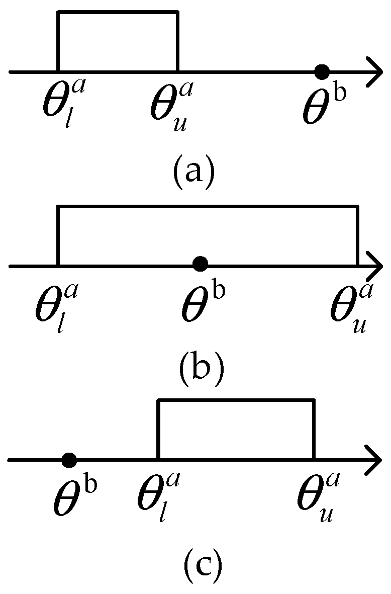
2.3. Possibility Theory
3. Improved Model
3.1. Interval DEA Improvement Model
3.2. Improving DEA Model with Possibility Theory
3.3. Model Steps and Properties
4. Illustrations
4.1. Numerical Examples
4.2. Airline Efficiency Evaluations
5. Conclusions
Author Contributions
Funding
Data Availability Statement
Conflicts of Interest
References
- Falavigna, G.; Ippoliti, R. The socio-economic planning of a community nurses programme in mountain areas: A Directional Distance Function approach. Socio-Econ. Plan. Sci. 2020, 71, 100770. [Google Scholar] [CrossRef]
- Gao, X.; Huang, L.; Wang, H. Spatiotemporal differentiation and convergence characteristics of green economic efficiency in China: From the perspective of pollution and carbon emission reduction. Environ. Sci. Pollut. Res. 2023, 30, 109525–109545. [Google Scholar] [CrossRef]
- Boccali, F.; Mariani, M.M.; Visani, F.; Mora-Cruz, A. Innovative value-based price assessment in data-rich environments: Leveraging online review analytics through Data Envelopment Analysis to empower managers and entrepreneurs. Technol. Forecast. Soc. Chang. 2022, 182, 121807. [Google Scholar] [CrossRef]
- Cheng, G.; Zervopoulos, P.D. Estimating the technical efficiency of health care systems: A cross-country comparison using the directional distance function. Eur. J. Oper. Res. 2014, 238, 899–910. [Google Scholar] [CrossRef]
- Mohammad, T.; Mahsa, G.; Masoud, T. Rang-adjusted measure: Modelling and computational aspects from internal and external perspectives for network DEA. Oper. Res. 2023, 23, 62. [Google Scholar]
- Hyok, K.N.; Feng, H.; Chol, K.O. Combining common-weights DEA window with the Malmquist index: A case of China’s iron and steel industry. Socio-Econ. Plan. Sci. 2023, 87, 101596. [Google Scholar]
- Huan, L.L.; Lei, C.; Yu, C. A new cross-efficiency DEA approach for measuring the safety efficiency of China's construction industry. Kybernetes 2023, 52, 6379–6394. [Google Scholar]
- Xiong, B.; Zou, Y.; An, Q.; Yan, X. Cross-direction environmental performance evaluation based on directional distance function in data envelopment analysis. Expert Syst. Appl. 2022, 203, 117327. [Google Scholar] [CrossRef]
- Oliveira, M.S.d.; Lizot, M.; Siqueira, H.; Afonso, P.; Trojan, F. Efficiency analysis of oil refineries using DEA window analysis, cluster analysis, and Malmquist productivity index. Sustainability 2023, 15, 13611. [Google Scholar] [CrossRef]
- Yan, Z.; Zhou, W.; Wang, Y.; Chen, X. Comprehensive Analysis of Grain Production Based on Three-Stage Super-SBM DEA and Machine Learning in Hexi Corridor, China. Sustainability 2022, 14, 8881. [Google Scholar] [CrossRef]
- Liu, J.S.; Lu, L.Y.Y.; Lu, W.-M. Research fronts in data envelopment analysis. Omega 2016, 58, 33–45. [Google Scholar] [CrossRef]
- Izadikhah, M.; Farzipoor Saen, R. A new data envelopment analysis method for ranking decision making units: An application in industrial parks. Expert Syst. 2015, 32, 596–608. [Google Scholar] [CrossRef]
- An, Q.; Meng, F.; Xiong, B. Interval cross efficiency for fully ranking decision making units using DEA/AHP approach. Ann. Oper. Res. 2018, 271, 297–317. [Google Scholar] [CrossRef]
- Kritikos, M.N. A full ranking methodology in data envelopment analysis based on a set of dummy decision making units. Expert Syst. Appl. 2017, 77, 211–225. [Google Scholar] [CrossRef]
- Jahanshahloo, G.R.; Memariani, A.; Lotfi, F.H.; Rezai, H.Z. A note on some of DEA models and finding efficiency and complete ranking using common set of weights. Appl. Math. Comput. 2005, 166, 265–281. [Google Scholar] [CrossRef]
- Ekiz, M.K.; Tuncer Şakar, C. A new DEA approach to fully rank DMUs with an application to MBA programs. Int. Trans. Oper. Res. 2019, 27, 1886–1910. [Google Scholar] [CrossRef]
- Arana-Jiménez, M.; Lozano-Ramírez, J.; Sánchez-Gil, M.C.; Younesi, A.; Lozano, S. A Novel Slacks-Based Interval DEA Model and Application. Axioms 2024, 13, 144. [Google Scholar] [CrossRef]
- Wei, B.-w.; Ma, Y.-y.; Ji, A.-b. Stage interval ratio DEA models and applications. Expert Syst. Appl. 2024, 238, 122397. [Google Scholar] [CrossRef]
- Lei, X.; Li, Y.; Morton, A. Dominance and ranking interval in DEA parallel production systems. OR Spectr. 2021, 44, 649–675. [Google Scholar] [CrossRef]
- Arabmaldar, A.; Kwasi Mensah, E.; Toloo, M. Robust worst-practice interval DEA with non-discretionary factors. Expert Syst. Appl. 2021, 182, 115256. [Google Scholar] [CrossRef]
- Toloo, M.; Keshavarz, E.; Hatami-Marbini, A. An interval efficiency analysis with dual-role factors. OR Spectr. 2020, 43, 255–287. [Google Scholar] [CrossRef]
- Sexton, T.R.; Silkman, R.H.; Hogan, A.J. Data envelopment analysis: Critique and extensions. New Dir. Program Eval. 1986, 1986, 73–105. [Google Scholar] [CrossRef]
- Dominikos, K.M.; Patrick, B.; Jonathan, K. A ranking framework based on interval self and cross-efficiencies in a two-stage DEA system. RAIRO Oper. Res. 2022, 56, 1293–1319. [Google Scholar]
- Ruiz, L.J. Cross-efficiency evaluation with directional distance functions. Eur. J. Oper. Res. 2013, 228, 181–189. [Google Scholar] [CrossRef]
- Chen, L.; Huang, Y.; Li, M.J.; Wang, Y.M. Meta-frontier analysis using cross-efficiency method for performance evaluation. Eur. J. Oper. Res. 2020, 280, 219–229. [Google Scholar] [CrossRef]
- Wu, J.; Chu, J.; Sun, J.; Zhu, Q. DEA cross-efficiency evaluation based on Pareto improvement. Eur. J. Oper. Res. 2016, 248, 571–579. [Google Scholar] [CrossRef]
- Lin, R.; Tu, C. Cross-efficiency evaluation and decomposition with directional distance function in series and parallel systems. Expert Syst. Appl. 2021, 177, 114933. [Google Scholar]
- Andersen, P.; Petersen, N.C. A procedure for ranking efficient units in data envelopment analysis. Manag. Sci. 1993, 39, 1261–1264. [Google Scholar] [CrossRef]
- Xie, Q.; Zhang, L.L.; Shang, H.; Emrouznejad, A.; Li, Y. Evaluating performance of super-efficiency models in ranking efficient decision-making units based on Monte Carlo simulations. Ann. Oper. Res. 2021, 305, 273–323. [Google Scholar] [CrossRef]
- Qu, J.; Wang, B.; Liu, X. A modified super-efficiency network data envelopment analysis: Assessing regional sustainability performance in China. Socio-Econ. Plan. Sci. 2022, 82, 101262. [Google Scholar] [CrossRef]
- Yan, Y.; Chen, Y.; Han, M.; Zhen, H. Research on Energy Efficiency Evaluation of Provinces along the Belt and Road under Carbon Emission Constraints: Based on Super-Efficient SBM and Malmquist Index Model. Sustainability 2022, 14, 8453. [Google Scholar] [CrossRef]
- Hongjun, G.; Yu, W.; Liye, D.; Aiwu, Z. Efficiency Decomposition Analysis of the Marine Ship Industry Chain Based on Three-Stage Super-Efficiency SBM Model—Evidence from Chinese A-Share-Listed Companies. Sustainability 2022, 14, 12155. [Google Scholar]
- Nakahara, Y.; Sasaki, M.; Gen, M. On the linear programming problems with interval coefficients. Computers 1992, 23, 301–304. [Google Scholar] [CrossRef]
- Facchinetti, G.; Ricci, R.G.; Muzzioli, S. Note on ranking fuzzy triangular numbers. Int. J. Intell. Syst. 1998, 13, 613–622. [Google Scholar] [CrossRef]
- Lan, Y.; Wen, B.; Wang, Y. A common-weights interval DEA approach for efficiency evaluation and its ranking method. Oper. Res. Trans. 2021, 25, 58–68. [Google Scholar]
- Song, L.; Liu, F. An improvement in DEA cross-efficiency aggregation based on the Shannon entropy. Int. Trans. Oper. Res. 2018, 25, 705–714. [Google Scholar] [CrossRef]
- Chen, L.; Wang, Y. Cross-Efficiency Aggregation Method Based on Prospect Theory. J. Syst. Sci. Math. Sci. 2018, 38, 1307. [Google Scholar]
- Zhang, Q.; Fan, Z.; Pan, D.H. A Ranking Approach for Interval Numbers in Uncertain Multiple Attribute Decision Making Problems. Syst. Eng. Theory Parct. 1999, 5, 130–134. [Google Scholar]
- Ke, L.; Tang, H.; Wang, Q. Ranking Method of Interval Numbers Based on Possibility Function of Binary Connection Number and Its Applica. J. Syst. Sci. Math. Sci. 2023, 43, 417–430. [Google Scholar]
- Sun, B.; Zeng, Y.; Su, Z. Task allocation in multi-AUV dynamic game based on interval ranking under uncertain information. Ocean Eng. 2023, 288, 116057. [Google Scholar] [CrossRef]
- Ta, N.; Zheng, Z.; Xie, H. An interval particle swarm optimization method for interval nonlinear uncertain optimization problems. Adv. Mech. Eng. 2023, 15, 16878132231153266. [Google Scholar] [CrossRef]
- Liu, F.; Pan, L.H.; Liu, Z.L.; Peng, Y.N. On possibility-degree formulae for ranking interval numbers. Soft Comput. 2018, 22, 2557–2565. [Google Scholar] [CrossRef]
- Charnes, A.; Cooper, W.W.; Rhodes, E. Measuring the efficiency of decision making units. Eur. J. Oper. Res. 1978, 2, 429–444. [Google Scholar] [CrossRef]
- Ghasemi, M.R.; Ignatius, J.; Rezaee, B. Improving discriminating power in data envelopment models based on deviation variables framework. Eur. J. Oper. Res. 2019, 278, 442–447. [Google Scholar] [CrossRef]
- Moore, R. Interval Analysis; Prentice-Hall: Englewood Cliffs, NJ, USA, 1966. [Google Scholar]
- Da, Q.; Liu, X. Interval number linear programming and its satisfactory solution. Syst. Eng. Theory Pract. 1999, 19, 3–7. [Google Scholar]
- Xu, Z.; Da, Q. Possibility degree method for ranking interval numbers and its application. J. Syst. Eng. 2003, 18, 67–70. [Google Scholar]
- Wang, Y.M.; Yang, J.B.; Xu, D.L. A two-stage logarithmic goal programming method for generating weights from interval comparison matrices. Fuzzy Sets Syst. 2004, 152, 475–498. [Google Scholar] [CrossRef]
- Sun, H.; Yao, W. Comments on methods for ranking interval numbers. J. Syst. Eng. 2010, 25, 18–26. [Google Scholar]
- Liu, F. Acceptable consistency analysis of interval reciprocal comparison matrices. Fuzzy Sets Syst. 2009, 160, 2686–2700. [Google Scholar] [CrossRef]
- Ang, S.; Fan, T.-t.; Yang, F. DEA Model for Fixed Cost Allocation in Two-stage Systems Based on Fairness. Oper. Res. Manag. Sci. 2022, 31, 93. [Google Scholar]
- Wong, Y.-H.B.; Beasley, J.E. Restricting weight flexibility in data envelopment analysis. J. Oper. Res. Soc. 1990, 41, 829–835. [Google Scholar] [CrossRef]
- Ngo, T.; Tsui, K.W.H. Estimating the confidence intervals for DEA efficiency scores of Asia-Pacific airlines. Oper. Res. 2021, 22, 3411–3434. [Google Scholar] [CrossRef]
- Lee, B.L.; Worthington, A.C. Technical efficiency of mainstream airlines and low-cost carriers: New evidence using bootstrap data envelopment analysis truncated regression. J. Air Transp. Manag. 2014, 38, 15–20. [Google Scholar] [CrossRef]
- Min, H.; Joo, S.-J. A comparative performance analysis of airline strategic alliances using data envelopment analysis. J. Air Transp. Manag. 2016, 52, 99–110. [Google Scholar] [CrossRef]
- Barbot, C.; Costa, Á.; Sochirca, E. Airlines performance in the new market context: A comparative productivity and efficiency analysis. J. Air Transp. Manag. 2008, 14, 270–274. [Google Scholar] [CrossRef]


| DMU | x1 | x2 | x3 | y1 | y2 | y3 |
|---|---|---|---|---|---|---|
| 1 | 12 | 400 | 20 | 60 | 35 | 17 |
| 2 | 19 | 750 | 70 | 139 | 41 | 40 |
| 3 | 42 | 1500 | 70 | 225 | 68 | 75 |
| 4 | 15 | 600 | 100 | 90 | 12 | 17 |
| 5 | 45 | 2000 | 250 | 253 | 145 | 130 |
| 6 | 19 | 730 | 50 | 132 | 45 | 45 |
| 7 | 41 | 2350 | 600 | 305 | 159 | 97 |
| DMU | 1 | 2 | 3 | 4 | 5 | 6 | 7 |
|---|---|---|---|---|---|---|---|
| Selfish model (13) | 1 | 1 | 1 | 0.82 | 1 | 1 | 1 |
| Non-selfish model (15) | −10.1524 | 1.336643 | 5.268163 | −1.57278 | 7.280709 | 0.993284 | 7.099546 |
| DMU | 1 | 2 | 3 | 4 | 5 | 6 | 7 |
|---|---|---|---|---|---|---|---|
| Interval efficiency | [0,1] | [0.6590,1] | [0.8846,1] | [0.4291,0.82] | [1,1] | [0.6393,1] | [0.9896,1] |
| DMU | 1 | 2 | 3 | 4 | 5 | 6 | 7 | Sum |
|---|---|---|---|---|---|---|---|---|
| 1 | 0.5 | 0.146722 | 0.046936 | 0.301884 | 0 | 0.155947 | 0.00411 | 1.1556 |
| 2 | 0.853278 | 0.5 | 0.159949 | 0.883573 | 0 | 0.529575 | 0.014007 | 2.940381 |
| 3 | 0.953064 | 0.840051 | 0.5 | 1 | 0 | 0.849512 | 0.043786 | 4.186413 |
| 4 | 0.698116 | 0.116427 | 0 | 0.5 | 0 | 0.139267 | 0 | 1.453811 |
| 5 | 1 | 1 | 1 | 1 | 0.5 | 1 | 1 | 6.5 |
| 6 | 0.844053 | 0.470425 | 0.150488 | 0.860733 | 0 | 0.5 | 0.013179 | 2.838878 |
| 7 | 0.99589 | 0.985993 | 0.956214 | 1 | 0 | 0.986821 | 0.5 | 5.424918 |
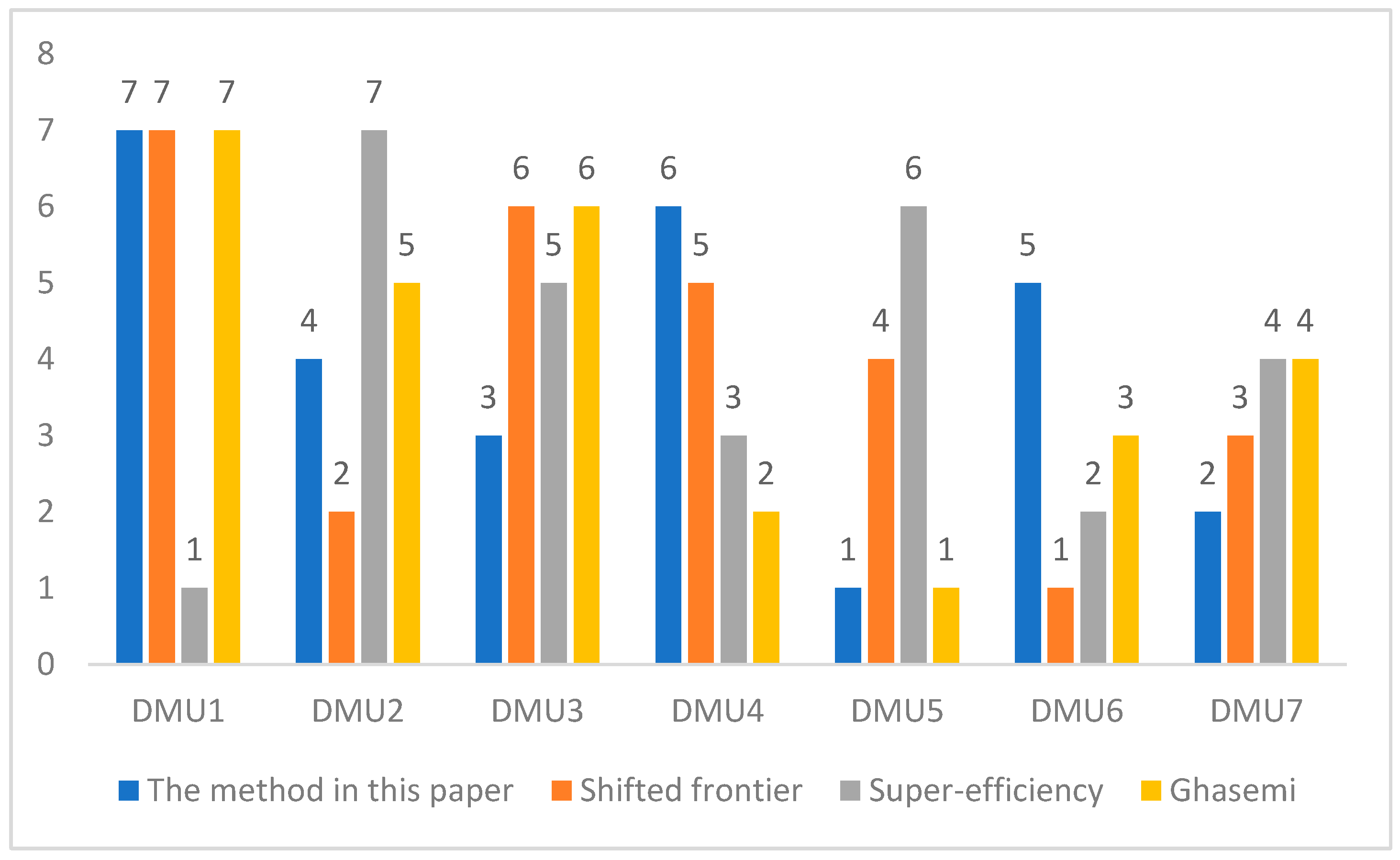
| DMU | CCR | Shifted Frontier | Super-Efficiency | Ghasemi | The Proposed Method | |||
|---|---|---|---|---|---|---|---|---|
| Eff. Values | Eff. Values | Rank | Eff. Values | Rank | Eff. Values | Rank | Rank | |
| DMU1 | 1 | 0.20683 | 7 | 1.829615 | 1 | 0.218 | 7 | 7 |
| DMU2 | 1 | 0.270049 | 2 | 1.048895 | 7 | 0.145 | 5 | 4 |
| DMU3 | 1 | 0.197749 | 6 | 1.198308 | 5 | 0.805 | 6 | 3 |
| DMU4 | 0.82 | 0.221479 | 5 | 0.819737 | 3 | - | 2 | 6 |
| DMU5 | 1 | 0.250576 | 4 | 1.219992 | 6 | 0.049 | 1 | 1 |
| DMU6 | 1 | 0.25645 | 1 | 1.190642 | 2 | 0.126 | 3 | 5 |
| DMU7 | 1 | 0.277708 | 3 | 1.266094 | 4 | 0.045 | 4 | 2 |
| Representative Study | Input Indicators | Output Indicators |
|---|---|---|
| Ngo and Tsui [53] | Available seat-kilometers (ASK) Available tonne-kilometers (ATK) Operating expenses (EXPENSES) | Revenue passenger-kilometers (RPK) Revenue tonne-kilometers (RTK) Operating revenues (REVENUES) |
| Lee and Worthington [54] | The average number of employees Total assets in USD Kilometers flown | Available tonne-kilometers (ATK) |
| Min and Joo [55] | Underutilization Operating expenses | Passengers RPKs Operating revenue Service rating |
| Barbot et al. [56] | Labor Capital (the airline’s fleet) Fuel Other operating inputs | Passenger service Cargo service Ancillary output |
| Indicators | Explanation | |
|---|---|---|
| Input indicators | Number of take-offs (unit: aircraft) | The aggregate number of aircraft sorties within a designated period of time. |
| Flight hours (unit: hours) | The duration of the aircraft flying time. | |
| Output indicators | Passenger volume (unit: individuals) | The actual number of passengers transported within a specific period. |
| Passenger turnover (unit: 10,000 passenger-kilometers) | The passenger turnover reflects the total volume of passenger transportation work during a specific period. | |
| Cargo volume (unit: tons) | The freight transport volume represents the actual quantity of goods transported during a specific period. | |
| Cargo turnover (unit: 10,000 ton-kilometers) | The freight turnover reflects the total volume of goods transportation work during a specific period. |
| Airlines | Before Normalization | After Normalization | ||
|---|---|---|---|---|
| Efficiency Upper Bound | Efficiency Lower Bound | Efficiency Upper Bound | Efficiency Lower Bound | |
| China Southern Airlines | 1 | 7605.413 | 0.421488 | 1 |
| Air China | 0.977608 | 7602.522 | 0.421484 | 0.977608 |
| China Eastern Airlines | 0.858185 | 7603.034 | 0.421485 | 0.858185 |
| Sichuan Airlines | 0.905655 | 7593.871 | 0.421475 | 0.905655 |
| Xiamen Air | 0.857561 | 7594.547 | 0.421476 | 0.857561 |
| Shenzhen Airlines | 0.816271 | 7595.956 | 0.421477 | 0.816271 |
| Hainan Airlines | 0.989872 | 7589.414 | 0.42147 | 0.989872 |
| Spring Airlines | 1 | 7588.01 | 0.421468 | 1 |
| Shandong Airlines | 0.892908 | 7589.532 | 0.42147 | 0.892908 |
| Juneyao Airlines | 0.899937 | 7577.694 | 0.421457 | 0.899937 |
| Beijing Capital Airlines | 1 | 7567.888 | 0.421446 | 1 |
| Zhejiang Loong Airlines | 0.864505 | 7564.184 | 0.421442 | 0.864505 |
| China Eastern Airlines Yunnan Limited | 0.738032 | 7573.442 | 0.421452 | 0.738032 |
| Shanghai Airlines | 0.774332 | 7568.362 | 0.421447 | 0.774332 |
| China Eastern Airlines Jiangsu Limited | 0.780659 | 7566.109 | 0.421444 | 0.780659 |
| Lucky Air | 0.957777 | 7549.363 | 0.421426 | 0.957777 |
| Tianjin Airlines | 0.825296 | 7558.067 | 0.421436 | 0.825296 |
| West Air | 1 | 7539.486 | 0.421415 | 1 |
| Chengdu Airlines | 0.825793 | 7549.955 | 0.421427 | 0.825793 |
| Suparna Airlines | 1 | 7454.055 | 0.421321 | 1 |
| China Express | 0.592403 | 7565.231 | 0.421443 | 0.592403 |
| China Xinhua Airlines Group | 0.8613 | 7526.507 | 0.421401 | 0.8613 |
| China United | 0.684278 | 7546.518 | 0.421423 | 0.684278 |
| Hebei Airlines | 0.836645 | 7516.756 | 0.42139 | 0.836645 |
| China Southern Airlines Henan Limited | 0.84781 | 7518.408 | 0.421392 | 0.84781 |
| Tibet Airlines | 0.785782 | 7520.074 | 0.421394 | 0.785782 |
| Shenzhen Donghai Airlines | 0.910002 | 7500.322 | 0.421372 | 0.910002 |
| Kunming Airlines | 0.829705 | 7508.146 | 0.421381 | 0.829705 |
| 9 Air | 1 | 7484.573 | 0.421355 | 1 |
| Qingdao Airlines | 0.839825 | 7499.946 | 0.421372 | 0.839825 |
| Okay Airways | 0.944351 | 7477.43 | 0.421347 | 0.944351 |
| Ruili Airlines | 0.921448 | 7479.333 | 0.421349 | 0.921448 |
| Chongqing Airlines | 0.733775 | 7504.117 | 0.421376 | 0.733775 |
| Air Guizhou | 0.865709 | 7474.284 | 0.421344 | 0.865709 |
| China Eastern Airlines Wuhan Limited | 0.919896 | 7469.817 | 0.421339 | 0.919896 |
| Guangxi Airlines | 0.764911 | 7463.234 | 0.421331 | 0.764911 |
| Urumqi Air | 1 | 7330.962 | 0.421186 | 1 |
| Zhuhai Airlines | 0.792984 | 7418.66 | 0.421282 | 0.792984 |
| Fuzhou Airlines | 0.857159 | 7402.27 | 0.421264 | 0.857159 |
| Shantou Airlines | 0.821189 | 7420.001 | 0.421284 | 0.821189 |
| Air Changan | 0.951132 | 7358.437 | 0.421216 | 0.951132 |
| Dalian Airlines | 0.773927 | 7370.418 | 0.42123 | 0.773927 |
| Air Travel | 0.91094 | 7290.883 | 0.421142 | 0.91094 |
| Jiangxi Airlines | 0.855918 | 7303.761 | 0.421156 | 0.855918 |
| Air China Inner Mongolia | 0.820033 | 7350.895 | 0.421208 | 0.820033 |
| Air Guilin | 0.855987 | 7283.549 | 0.421134 | 0.855987 |
| Colorful Guizhou Airlines | 0.618158 | 7380.347 | 0.42124 | 0.618158 |
| Grand China Air | 0.924141 | 6267.371 | 0.420019 | 0.924141 |
| Longjiang Airlines | 0.804375 | 6227.493 | 0.419975 | 0.804375 |
| Beijing Airlines | 0.950829 | 6511.255 | 0.420286 | 0.950829 |
| Joyair | 0.421488 | 7020.024 | 0.420845 | 0.421488 |
| Genghis Khan Airlines | 0.541277 | 5500.45 | 0.419177 | 0.541277 |
| One Two Three | 0.50545 | -376311 | 0 | 0.50545 |
| China Southern Airlines | Air China | China Eastern Airlines | Sichuan Airlines | Xiamen Air | Shenzhen Airlines | Hainan Airlines | |
|---|---|---|---|---|---|---|---|
| China Southern Airlines | 0.5 | 0.519367 | 0.622623 | 0.58159 | 0.623171 | 0.658865 | 0.508774 |
| Air China | 0.480633 | 0.5 | 0.607416 | 0.56473 | 0.607986 | 0.645117 | 0.489219 |
| China Eastern Airlines | 0.377377 | 0.392584 | 0.5 | 0.450968 | 0.500726 | 0.548017 | 0.384124 |
| Sichuan Airlines | 0.41841 | 0.43527 | 0.549032 | 0.5 | 0.549687 | 0.592338 | 0.425888 |
| Xiamen Air | 0.376829 | 0.392014 | 0.499274 | 0.450313 | 0.5 | 0.547357 | 0.383566 |
| Shenzhen Airlines | 0.341135 | 0.354883 | 0.451983 | 0.407662 | 0.452643 | 0.5 | 0.347238 |
| Hainan Airlines | 0.491226 | 0.510781 | 0.615876 | 0.574112 | 0.616434 | 0.652762 | 0.5 |
| Airlines | Possibility Accumulation | Ranking |
|---|---|---|
| China Southern Airlines | 33.7404 | 1 |
| Air China | 32.96998 | 9 |
| China Eastern Airlines | 27.95349 | 25 |
| Sichuan Airlines | 30.1364 | 19 |
| Xiamen Air | 27.92244 | 26 |
| Shenzhen Airlines | 25.82609 | 38 |
| Hainan Airlines | 33.39712 | 8 |
| Spring Airlines | 33.73934 | 2 |
| Shandong Airlines | 29.57464 | 21 |
| Juneyao Airlines | 29.88564 | 20 |
| Beijing Capital Airlines | 33.73813 | 3 |
| Zhejiang Loong Airlines | 28.25687 | 23 |
| China Eastern Airlines Yunnan Limited | 21.53633 | 46 |
| Shanghai Airlines | 23.56419 | 43 |
| China Eastern Airlines Jiangsu Limited | 23.91198 | 42 |
| Lucky Air | 32.24218 | 10 |
| Tianjin Airlines | 26.29467 | 35 |
| West Air | 33.73641 | 4 |
| Chengdu Airlines | 26.31985 | 34 |
| Suparna Airlines | 33.73121 | 6 |
| China Express | 12.92083 | 50 |
| China Xinhua Airlines Group | 28.09983 | 24 |
| China United | 18.4483 | 48 |
| Hebei Airlines | 26.87465 | 32 |
| China Southern Airlines Henan Limited | 27.43652 | 30 |
| Tibet Airlines | 24.18898 | 41 |
| Shenzhen Donghai Airlines | 30.31785 | 18 |
| Kunming Airlines | 26.51913 | 33 |
| 9 Air | 33.73307 | 5 |
| Qingdao Airlines | 27.03476 | 31 |
| Okay Airways | 31.72312 | 13 |
| Ruili Airlines | 30.80009 | 15 |
| Chongqing Airlines | 21.2903 | 47 |
| Air Guizhou | 28.30871 | 22 |
| China Eastern Airlines Wuhan Limited | 30.73475 | 16 |
| Guangxi Airlines | 23.03551 | 45 |
| Urumqi Air | 33.72369 | 7 |
| Zhuhai Airlines | 24.57313 | 40 |
| Fuzhou Airlines | 27.89012 | 27 |
| Shantou Airlines | 26.07175 | 36 |
| Air Changan | 31.97793 | 11 |
| Dalian Airlines | 23.52835 | 44 |
| Air Travel | 30.34448 | 17 |
| Jiangxi Airlines | 27.82282 | 29 |
| Air China Inner Mongolia | 26.00671 | 37 |
| Air Guilin | 27.82484 | 28 |
| Colorful Guizhou Airlines | 14.49835 | 49 |
| Grand China Air | 30.83279 | 14 |
| Longjiang Airlines | 25.10228 | 39 |
| Beijing Airlines | 31.91201 | 12 |
| Joyair | 1.358619 | 53 |
| Genghis Khan Airlines | 9.517831 | 51 |
| One Two Three | 1.570545 | 52 |
Disclaimer/Publisher’s Note: The statements, opinions and data contained in all publications are solely those of the individual author(s) and contributor(s) and not of MDPI and/or the editor(s). MDPI and/or the editor(s) disclaim responsibility for any injury to people or property resulting from any ideas, methods, instructions or products referred to in the content. |
© 2024 by the authors. Licensee MDPI, Basel, Switzerland. This article is an open access article distributed under the terms and conditions of the Creative Commons Attribution (CC BY) license (https://creativecommons.org/licenses/by/4.0/).
Share and Cite
Yang, S.; Zhao, G.; Li, F. The Efficiency Evaluation of DEA Model Incorporating Improved Possibility Theory. Mathematics 2024, 12, 3116. https://doi.org/10.3390/math12193116
Yang S, Zhao G, Li F. The Efficiency Evaluation of DEA Model Incorporating Improved Possibility Theory. Mathematics. 2024; 12(19):3116. https://doi.org/10.3390/math12193116
Chicago/Turabian StyleYang, Shenzi, Guoqing Zhao, and Fan Li. 2024. "The Efficiency Evaluation of DEA Model Incorporating Improved Possibility Theory" Mathematics 12, no. 19: 3116. https://doi.org/10.3390/math12193116
APA StyleYang, S., Zhao, G., & Li, F. (2024). The Efficiency Evaluation of DEA Model Incorporating Improved Possibility Theory. Mathematics, 12(19), 3116. https://doi.org/10.3390/math12193116