General Trapezoidal-Type Inequalities in Fuzzy Settings

Abstract

In this study, trapezoidal-type inequalities in fuzzy settings have been investigated. The theory of fuzzy analysis has been discussed in detail. The integration by parts formula of analysis of fuzzy mathematics has been employed to establish an equality. Trapezoidal-type inequality for functions with values in the fuzzy number-valued space is proven by applying the proven equality together with the properties of a metric defined on the set of fuzzy number-valued space and Höler’s inequality. The results proved in this research provide generalizations of the results from earlier existing results in the field of mathematical inequalities. An example is designed by defining a function that has values in fuzzy number-valued space and validated the results numerically using the software Mathematica (latest v. 14.1). The p-levels of the defined fuzzy number-valued mapping have been shown graphically for different values of $p\in \left[0,1\right]$.

1. Introduction

Mathematical inequalities play an important role in proving several results in different areas of pure and applied mathematics. That is why this topic has emerged as an important topic in mathematics over the past several years, and mathematicians have successfully applied this subject to provide new generalizations, refine existing results, and even prove new results.

In classical analysis, a trapezoidal-type inequality is an inequality that provides upper and/or lower bounds for the quantity:

$${\displaystyle \frac{\nu \left(k\right)+\nu (\mathit{\ell })}{2}}\left(\mathit{\ell }-k\right)-{\int }_k^{\mathit{\ell }}\nu \left(t\right)dt,$$

(1)

that is the error in approximating the integral by a trapezoidal rule, for various classes of integrable functions $\nu$ defined on the compact interval $\left[k,\mathit{\ell }\right]$.

Cerone et al. obtained trapezoidal-type inequalities for functions of bounded variation in [1].

Theorem 1

([1]). Let $\nu :\left[k,\mathit{\ell }\right]\to \mathbb{C}$ be a function of bounded variation. We have the inequality

$$\left|{\int }_k^{\mathit{\ell }}\nu \left(t\right)dt-{\displaystyle \frac{\nu \left(k\right)+\nu (\mathit{\ell })}{2}}\left(\mathit{\ell }-k\right)\right|\le {\displaystyle \frac{1}{2}}\left(\mathit{\ell }-k\right)\stackrel{\mathit{\ell }}{\underset{k}{\vee }}\left(\nu \right),$$

(2)

where $\stackrel{\mathit{\ell }}{\underset{k}{\vee }}\left(\nu \right)$ denotes the total variation of ν on the interval $\left[k,\mathit{\ell }\right]$. The constant ${\displaystyle \frac{1}{2}}$ is the best possible one.

If the mapping $\nu$ is Lipschitzian, then the following result holds as well [2].

Theorem 2

([2]). Let $\nu :\left[k,\mathit{\ell }\right]\to \mathbb{C}$ be an L-Lipschitzian function on $\left[k,\mathit{\ell }\right]$, i.e., ν satisfies the condition:

$$\left|\nu \left(t\right)-\nu \left(s\right)\right|\le L{\left|t-s\right|}^u$$

for all $t,s\in \left[k,\mathit{\ell }\right],L>0$. Then, we have the inequality:

$$\left|{\int }_k^{\mathit{\ell }}\nu \left(t\right)dt-{\displaystyle \frac{\nu \left(k\right)+\nu (\mathit{\ell })}{2}}\left(\mathit{\ell }-k\right)\right|\le {\displaystyle \frac{1}{4}}{\left(\mathit{\ell }-k\right)}^{2}L.$$

(3)

The constant ${\displaystyle \frac{1}{4}}$ is best in (3).

With the assumption of absolute continuity for the function $\nu$, then the following estimates in terms of the Lebesgue norms of the derivative ${\nu }^{\prime }$ hold [3] (p. 93).

Theorem 3

([3]). Let $\nu :\left[k,\mathit{\ell }\right]\to \mathbb{C}$ be an absolutely continuous function on $\left[k,\mathit{\ell }\right]$. Then, we have

$$\begin{array}{cc}\left|{\int }_k^{\mathit{\ell }}\nu \left(t\right)dt-{\displaystyle \frac{\nu \left(k\right)+\nu (\mathit{\ell })}{2}}\left(\mathit{\ell }-k\right)\right|\hfill & \\ & \hfill \le \left\{\begin{array}{cc}{\displaystyle \frac{1}{4}}{\left(\mathit{\ell }-k\right)}^2{∥{\nu }^{\prime }∥}_{\infty },& if{\nu }^{\prime }\in L_{\infty }\left[k,\mathit{\ell }\right],\\ & \\ {\displaystyle \frac{1}{2{\left(r+1\right)}^{\frac{1}{r}}}}{\left(\mathit{\ell }-k\right)}^{1+{\displaystyle \frac{1}{r}}}{∥{\nu }^{\prime }∥}_w,& if{\nu }^{\prime }\in L_w\left[k,\mathit{\ell }\right],\\ & \\ {\displaystyle \frac{1}{2}}\left(\mathit{\ell }-k\right){∥{\nu }^{\prime }∥}_1,\end{array}\right.\end{array}$$

(4)

where $w,r>1$ with ${\displaystyle \frac{1}{w}}+{\displaystyle \frac{1}{r}}=1$ and ${∥·∥}_w$ ($w\in \left[1,\infty \right]$) are the Lebesgue norms, i.e.,

$${∥{\nu }^{\prime }∥}_{\infty }=ess\underset{s\in \left[k,\mathit{\ell }\right]}{sup}\left|{\nu }^{\prime }\left(s\right)\right|$$

and

$${∥{\nu }^{\prime }∥}_w:={\left({\int }_k^{\mathit{\ell }}{\left|{\nu }^{\prime }\left(s\right)\right|}^{w}ds\right)}^{{\displaystyle \frac{1}{w}}},w\ge 1.$$

The next is a result on trapezoidal-type inequalities for operator convex functions.

Definition 1

([4]). A continuous function $\nu :I\to \mathbb{R}$ is operator convex on the interval I if

$$\nu \left(\left(1-t\right)A+tB\right)\le \left(1-t\right)\nu \left(A\right)+t\nu \left(B\right)$$

(5)

holds in the operator order, for all $t\in \left[0,1\right]$, where A and B are self-adjoint operators in a Hilbert space $\left(H,〈·,·〉\right)$ with spectra $Sp\left(A\right),Sp\left(B\right)\subset I$.

Theorem 4

([4]). Let $\nu :C\subset E\to F$ (E, F are Banach spaces and C is an open subset of E) be an operator convex function on I and $A,B,A\ne B$, self-adjoint operators on H with $Sp\left(A\right),Sp\left(B\right)\subset I$. If ν is Gâteaux differentiable on $V=\left[A,B\right]:=\left\{\left(1-t\right)A+tB,t\in \left[0,1\right]\right\}$ and $\phi :\left[0,1\right]\to \left[0,\infty \right)$ is Lebesgue integrable and symmetric about ${\displaystyle \frac{1}{2}}$, that is $\phi \left(1-t\right)=\phi \left(t\right)$ for all $t\in \left[0,1\right]$, then

$$\begin{array}{c}0\le \left({\int }_0^1\phi \left(t\right)dt\right){\displaystyle \frac{\nu \left(A\right)+\nu \left(B\right)}{2}}-{\int }_0^1\phi \left(t\right)\nu \left(\left(1-t\right)A+tB\right)dt\hfill \\ \hfill \hspace{1em}\hspace{1em}\hspace{1em}\hspace{1em}\hspace{1em}\hspace{1em}\hspace{1em}\hspace{1em}\le {\displaystyle \frac{1}{2}}{\int }_0^1\left({\displaystyle \frac{1}{2}}-\left|t-{\displaystyle \frac{1}{2}}\right|\right)\phi \left(t\right)dt\left[▽{\nu }_B\left(B-A\right)-▽{\nu }_A\left(B-A\right)\right],\end{array}$$

(6)

where $▽{\nu }_B\left(V\right)$ is the Gâteaux derivative over C in the direction V connecting the operators A and B.

A particular result of the above result can be obtained by taking for $\phi \equiv 1$. Hence, for $\phi \equiv 1$, we obtain

$$\begin{array}{c}\hfill 0\le {\displaystyle \frac{\nu \left(A\right)+\nu \left(B\right)}{2}}-{\int }_0^1\nu \left(\left(1-t\right)A+tB\right)dt\le {\displaystyle \frac{1}{8}}\left[▽{\nu }_B\left(B-A\right)-▽{\nu }_A\left(B-A\right)\right].\end{array}$$

(7)

For some trapezoid operator inequalities in Hilbert spaces, see [5,6,7,8].

Definition 2

([9]). Let X be a complex Banach space. We say that the vector valued function $\nu :\left[k,\mathit{\ell }\right]\to X$ is strongly differentiable on the interval $\left(k,\mathit{\ell }\right)$ if the limit

$${\nu }^{\prime }\left(t\right)=\underset{h\to 0}{lim}{\displaystyle \frac{\nu \left(t+h\right)-\nu \left(t\right)}{h}}$$

exists in the norm topology for all $t\in \left(k,\mathit{\ell }\right)$.

The following weighted version of generalized trapezoid inequality involving two functions with one function that contains values in Banach spaces was proven in Dragomir [9].

Theorem 5

([10]). Assume that $\phi :\left[k,\mathit{\ell }\right]\to \mathbb{C}$ and $\nu :\left[k,\mathit{\ell }\right]\to X$ are continuous and ν is strongly differentiable on $\left(k,\mathit{\ell }\right)$, then for all $\lambda \in \left[k,\mathit{\ell }\right]$, then we have the following inequality:

$$∥\left({\int }_{\lambda }^{\mathit{\ell }}\phi \left(s\right)ds\right)\nu \left(\mathit{\ell }\right)+\left({\int }_k^{\lambda }\phi \left(s\right)ds\right)\nu \left(k\right)-{\int }_k^{\mathit{\ell }}\phi \left(t\right)\nu \left(t\right)dt∥\le C\left(\phi ,\nu ,\lambda \right),$$

(8)

where

$$C\left(\phi ,\nu ,\lambda \right):={\int }_{\lambda }^{\mathit{\ell }}\left({\int }_{\lambda }^t\left|\phi \left(s\right)\right|ds\right)∥{\nu }^{\prime }\left(t\right)∥dt+{\int }_k^{\lambda }\left({\int }_t^{\lambda }\left|\phi \left(s\right)\right|ds\right)∥{\nu }^{\prime }\left(t\right)∥dt.$$

Moreover, the following bounds for $C\left(\phi ,\nu ,\lambda \right)$ hold:

$$\begin{array}{c}C\left(\phi ,\nu ,\lambda \right)\hfill \\ \hspace{1em}\hspace{1em}\hspace{1em}\hspace{1em}\hspace{1em}\le \left\{\begin{array}{c}\left({\int }_{\lambda }^{\mathit{\ell }}\left|\phi \left(s\right)\right|ds\right)\left({\int }_{\lambda }^{\mathit{\ell }}∥{\nu }^{\prime }\left(t\right)∥dt\right)+\left({\int }_k^{\lambda }\left|\phi \left(s\right)\right|ds\right)\left({\int }_k^{\lambda }∥{\nu }^{\prime }\left(t\right)∥dt\right),\\ \\ {\left[{\int }_{\lambda }^{\mathit{\ell }}{\left({\int }_{\lambda }^t\left|\phi \left(s\right)\right|ds\right)}^{w}dt\right]}^{{\displaystyle \frac{1}{w}}}{\left({\int }_{\lambda }^{\mathit{\ell }}{∥{\nu }^{\prime }\left(t\right)∥}^{r}dt\right)}^{{\displaystyle \frac{1}{r}}}\\ +{\left[{\int }_k^{\lambda }{\left({\int }_t^{\lambda }\left|\phi \left(s\right)\right|ds\right)}^{w}dt\right]}^{{\displaystyle \frac{1}{w}}}{\left({\int }_k^{\lambda }{∥{\nu }^{\prime }\left(t\right)∥}^{r}dt\right)}^{{\displaystyle \frac{1}{r}}},\\ \\ \left[{\int }_{\lambda }^{\mathit{\ell }}\left({\int }_{\lambda }^t\left|\phi \left(s\right)\right|ds\right)dt\right]{\displaystyle \underset{t\in \left[\lambda ,\mathit{\ell }\right]}{sup}}∥{\nu }^{\prime }\left(t\right)∥\\ +\left[{\int }_k^{\lambda }\left({\int }_t^{\lambda }\left|\phi \left(s\right)\right|ds\right)dt\right]{\displaystyle \underset{t\in \left[k,\lambda \right]}{sup}}∥{\nu }^{\prime }\left(t\right)∥,\end{array}\right.\hfill \end{array}$$

(9)

where $w,r>1$ with ${\displaystyle \frac{1}{w}}+{\displaystyle \frac{1}{r}}=1$.

A dual result for Theorem 5 is given as follows:

Theorem 6

([9]). Assume that $\phi :\left[k,\mathit{\ell }\right]\to \mathbb{C}$ and $\nu :\left[k,\mathit{\ell }\right]\to X$ are continuous and φ is continuously differentiable on $\left(k,\mathit{\ell }\right)$, then for all $\lambda \in \left[k,\mathit{\ell }\right]$ the inequality

$$∥\left({\int }_{\lambda }^{\mathit{\ell }}\nu \left(s\right)ds\right)\phi \left(\mathit{\ell }\right)+\left({\int }_k^{\lambda }\nu \left(s\right)ds\right)\phi \left(k\right)-{\int }_k^{\mathit{\ell }}\phi \left(t\right)\nu \left(t\right)dt∥\le \tilde{C}\left(\phi ,\nu ,\lambda \right),$$

(10)

where

$$\tilde{C}\left(\phi ,\nu ,\lambda \right)\le {\int }_{\lambda }^{\mathit{\ell }}\left({\int }_{\lambda }^t∥\nu \left(s\right)∥ds\right)\left|{\phi }^{\prime }\left(t\right)\right|dt+{\int }_k^{\lambda }\left({\int }_t^{\lambda }∥\nu \left(s\right)∥ds\right)\left|{\phi }^{\prime }\left(t\right)\right|dt$$

The following bounds hold for $\tilde{C}\left(\phi ,\nu ,\lambda \right)$:

$$\begin{array}{c}\tilde{C}\left(\phi ,\nu ,\lambda \right)\hfill \\ \hspace{1em}\hspace{1em}\hspace{1em}\hspace{1em}\hspace{1em}\le \left\{\begin{array}{c}{\int }_{\lambda }^{\mathit{\ell }}∥\nu \left(s\right)∥ds{\int }_{\lambda }^{\mathit{\ell }}\left|{\phi }^{\prime }\left(t\right)\right|dt+{\int }_k^{\lambda }\left|\nu \left(s\right)\right|ds{\int }_k^{\lambda }\left|{\phi }^{\prime }\left(t\right)\right|dt,\\ \\ {\left[{\int }_{\lambda }^{\mathit{\ell }}{\left({\int }_{\lambda }^t∥\nu \left(s\right)∥ds\right)}^{w}dt\right]}^{{\displaystyle \frac{1}{w}}}{\left({\int }_{\lambda }^{\mathit{\ell }}{\left|{\phi }^{\prime }\left(t\right)\right|}^{r}dt\right)}^{{\displaystyle \frac{1}{r}}}\\ +{\left[{\int }_k^{\lambda }{\left({\int }_t^{\lambda }∥\nu \left(s\right)∥ds\right)}^{w}dt\right]}^{{\displaystyle \frac{1}{w}}}{\left({\int }_k^{\lambda }{\left|{\phi }^{\prime }\left(t\right)\right|}^{r}dt\right)}^{{\displaystyle \frac{1}{r}}},\\ \\ {\displaystyle \underset{t\in \left[\lambda ,\mathit{\ell }\right]}{sup}}\left|{\phi }^{\prime }\left(s\right)\right|{\int }_{\lambda }^{\mathit{\ell }}\left({\int }_{\lambda }^t∥\nu \left(s\right)∥ds\right)dt\\ +{\displaystyle \underset{t\in \left[k,\lambda \right]}{sup}}\left|{\phi }^{\prime }\left(s\right)\right|{\int }_k^{\lambda }\left({\int }_t^{\lambda }∥\nu \left(s\right)∥ds\right)dt,\end{array}\right.\hfill \end{array}$$

(11)

where $w,r>1$ with ${\displaystyle \frac{1}{w}}+{\displaystyle \frac{1}{r}}=1$.

This study contains trapezoidal-type inequalities for fuzzy number-valued functions that can be seen as the most general inequalities of the trapezoidal type in this field so far. The inequalities proven in this paper not only generalize the earlier studies for trapezoidal-type inequalities for functions having values in the set of real numbers but also extend those studies that have been established for functions with values in Banach spaces. The results of this paper extend the results of Theorems 5 and 6 to fuzzy settings and hence also generalize the results of Theorem 3. The novelty of the results presented in this study is that they have not been previously investigated in any studies related to fuzzy environments. The researchers can uncover significant extensions and numerous applications in the mathematical sciences and other areas of science related to fuzzy mathematics. More recent studies on Ostrowski-, trapezoidal-, and midpoint-type inequalities can be explored in [11,12,13,14,15,16,17,18,19,20] and the references cited in these researches.

The next section is devoted to the basic definitions and results of fuzzy numbers and fuzzy number-valued functions.

2. Preliminaries

In this section we point out some basic definitions and results which would help us in the sequel of this paper, we begin with the following:

Definition 3 

([21]). Let us denote by ${\mathbb{R}}_{\mathcal{F}}$ the class of fuzzy subsets of real axis $\mathbb{R}$ (i.e., $\alpha :\mathbb{R}⟶\left[0,1\right]$), satisfying the following properties:

(i) 

$\forall \alpha \in {\mathbb{R}}_{\mathcal{F}},$ α is normal, i.e., with $\alpha \left(\tau \right)=1$ for some $\tau \in \mathbb{R}$.

(ii) 

$\forall \alpha \in {\mathbb{R}}_{\mathcal{F}},$ α is convex fuzzy set, i.e.,

$$\alpha (t\tau +(1-t)\overline{\tau })\ge min\left\{\alpha \left(\tau \right),\alpha \left(\overline{\tau }\right)\right\},\forall t\in [0,1],\forall \tau ,\overline{\tau }\in \mathbb{R}.$$

(iii) 

∀$\alpha \in$${\mathbb{R}}_{\mathcal{F}},$ α is upper semi-continuous on $\mathbb{R}$.

(iv) 

$\overline{\left\{\tau \in \mathbb{R}:\alpha \left(\tau \right)>0\right\}}$ is compact.

The set ${\mathbb{R}}_{\mathcal{F}}$ is called the space of fuzzy real numbers.

Remark 1.

It is clear that $\mathbb{R}\subset {\mathbb{R}}_{\mathcal{F}}$, because any real number ${\tau }_0\in \mathbb{R}$, can be described as the fuzzy number whose value is 1 for $\tau ={\tau }_0$ and zero otherwise.

It is clear that $\mathbb{R}\subset {\mathbb{R}}_{\mathcal{F}}$, because any real number ${\tau }_0\in \mathbb{R}$, can be described as the fuzzy number whose value is 1 for $\tau ={\tau }_0$ and zero otherwise. We will collect some further definitions and notations as needed in the sequel [22].

For $0<p\le 1$ and $\alpha \in {\mathbb{R}}_F$, we define

$${\left[\alpha \right]}^p=\left\{\tau \in \mathbb{R}:\alpha \left(\tau \right)\ge p\right\}$$

and

$${\left[\alpha \right]}^0=\overline{\left\{\tau \in \mathbb{R}:\alpha \left(\tau \right)>0\right\}}.$$

Now, it is well known that for each $p\in \left[0,1\right],$${\left[\alpha \right]}^p$, is a bounded closed interval. For $\alpha ,\gamma \in {\mathbb{R}}_{\mathcal{F}}$ and $\lambda \in \mathbb{R}$, we have the sum $\alpha \oplus \gamma$ and the product $\lambda \odot \alpha$ are defined by ${\left[\alpha \oplus \gamma \right]}^p={\left[\alpha \right]}^p+{\left[\gamma \right]}^p$, ${\left[\lambda \odot \alpha \right]}^p=\lambda {\left[\alpha \right]}^p,$$\forall p\in \left[0,1\right]$, where ${\left[\alpha \right]}^p+{\left[\gamma \right]}^p$ means the usual addition of two intervals as subsets of $\mathbb{R}$ and $\lambda {\left[\alpha \right]}^p$ means the usual product between a scalar and a subset of $\mathbb{R}$. It should be noted that the intervals ${[\alpha \oplus \gamma ]}^p$ and ${[\lambda \odot \alpha ]}^p$ uniquely determine the sum $\alpha \oplus \gamma$ of fuzzy numbers $\alpha$ and $\gamma$, and the product $\lambda \odot \alpha$ of a real number $\lambda$ and a fuzzy number $\alpha$.

• Now, we define $\mathcal{D}:{\mathbb{R}}_{\mathcal{F}}\times {\mathbb{R}}_{\mathcal{F}}⟶\mathbb{R}\cup \left\{0\right\}$ by

$$\mathcal{D}(\alpha ,\gamma )=\underset{p\in \left[0,1\right]}{sup}\left(max\left\{\left|{\alpha }_{-}^p-{\gamma }_{-}^p\right|,\left|{\alpha }_{+}^p-{\gamma }_{+}^p\right|\right\}\right),$$

where ${\left[\alpha \right]}^p=\left[{\alpha }_{-}^p,{\alpha }_{+}^p\right],$${\left[\gamma \right]}^p=\left[{\gamma }_{-}^p,{\gamma }_{+}^p\right],$ then $(\mathcal{D},{\mathbb{R}}_{\mathcal{F}})$ is a metric space and it possesses the following properties:

(i)

$\mathcal{D}(\alpha \oplus \beta ,\gamma \oplus \beta )=\mathcal{D}(\alpha ,\gamma ),$$\forall \alpha ,\gamma ,\beta \in {\mathbb{R}}_{\mathcal{F}}.$

(ii)

$\mathcal{D}(\lambda \odot$$\alpha ,$$\lambda \odot \gamma )=$$\lambda \mathcal{D}(\alpha ,\gamma ),\forall \alpha ,\gamma \in {\mathbb{R}}_{\mathcal{F}},\forall \lambda \in \mathbb{R}.$

(iii)

$\mathcal{D}(\alpha \oplus \gamma ,\beta \oplus e)\le \mathcal{D}(\alpha ,\beta )+\mathcal{D}(\gamma ,e),$$\forall \alpha ,\gamma ,\beta ,e\in {\mathbb{R}}_{\mathcal{F}}$

Moreover, it is well known that $({\mathbb{R}}_{\mathcal{F}},\mathcal{D})$ is a complete metric space.

Also we have the following theorem:

Theorem 7 

([23]). We have the following properties of a fuzzy number:

(i) 

If we denote $\tilde{o}={\mathcal{X}}_{\left\{0\right\}}$, then $\tilde{o}$$\in {\mathbb{R}}_{\mathcal{F}}$ is neutral element with respect to ⊕, i.e., $\alpha \oplus \tilde{o}=\tilde{o}\oplus \alpha$, for all $\alpha \in {\mathbb{R}}_{\mathcal{F}}$.

(ii) 

With respect to $\tilde{0}$ none of $\alpha \in {\mathbb{R}}_{\mathcal{F}}\setminus \mathbb{R}$ has opposite in ${\mathbb{R}}_{\mathcal{F}}$ with respect to ⊕.

(iii) 

For any $k,\mathit{\ell }\in \mathbb{R}$ with $k,\mathit{\ell }\ge 0$ or $k,\mathit{\ell }\le 0$, any $\alpha \in {\mathbb{R}}_{\mathcal{F}}$, we have $(k+\mathit{\ell })\odot \alpha =k\odot \alpha \oplus \mathit{\ell }\odot$$\alpha \forall k,\mathit{\ell }\in \mathbb{R}$ the above property does not hold.

(iv) 

For any $\lambda \in \mathbb{R}$ and any $\alpha ,\gamma \in {\mathbb{R}}_{\mathcal{F}},$ we have $\lambda \odot (\alpha \oplus \gamma )=\lambda \odot \alpha \oplus \lambda \odot \gamma .$

(v) 

For any $\lambda ,\mu \in \mathbb{R}$ and any $\alpha \in {\mathbb{R}}_{\mathcal{F}},$ we have $\lambda \odot (\mu \odot \gamma )=(\lambda ·\mu )\odot \gamma .$

(vi) 

If we denote ${∥\alpha ∥}_{\mathcal{F}}=\mathcal{D}(\alpha ,\tilde{o}),$$\forall \alpha \in {\mathbb{R}}_{\mathcal{F}}$ then ${∥.∥}_{\mathcal{F}}$ has the properties of a usual norm on ${\mathbb{R}}_{\mathcal{F}}$, i.e., ${∥\alpha ∥}_{\mathcal{F}}=0$ if and only if $\alpha =\tilde{o}$, ${∥\lambda \odot \alpha ∥}_{\mathcal{F}}=\left|\lambda \right|·{∥\alpha ∥}_{\mathcal{F}}$ and ${∥\alpha \oplus \gamma ∥}_{\mathcal{F}}\le {∥\alpha ∥}_{\mathcal{F}}+{∥\gamma ∥}_{\mathcal{F}},\left|{∥\alpha ∥}_{\mathcal{F}}-{∥\gamma ∥}_{\mathcal{F}}\right|\le \mathcal{D}(\alpha ,\gamma ).$

Remark 2.

The propositions (ii) and (iii) in theorem show us that $({\mathbb{R}}_{\mathcal{F}},\oplus ,\odot )$ is not a vector space over $\mathbb{R}$ and consequently $({\mathbb{R}}_{\mathcal{F}},{∥·∥}_{\mathcal{F}})$ cannot be a normed space. However, the properties of D and those in theorem (iv)–(vi), have the effect that most of the metric properties of functions defined as $\mathbb{R}$ with values in a Banach space can be extended to functions $\nu :\mathbb{R}⟶{\mathbb{R}}_{\mathcal{F}}$, called fuzzy number-valued functions.

In this paper, for the ranking concept, we will use a partial ordering which was introduced in [24].

Definition 4

([24]). Let the partial ordering ≼ in ${\mathbb{R}}_{\mathcal{F}}$ by $\alpha \preccurlyeq \gamma$ if and only if ${\alpha }_{-}^p\le {\gamma }_{-}^p$ and ${\alpha }_{+}^p\le {\gamma }_{+}^p$, $\forall p\in \left[0,1\right]$, and the strict inequality ≺ in ${\mathbb{R}}_{\mathcal{F}}$ is defined by $\alpha \prec \gamma$ if and only if ${\alpha }_{-}^p<{\gamma }_{-}^p$ and ${\alpha }_{+}^p<{\gamma }_{+}^p$, $\forall p\in \left[0,1\right]$, where ${\left[\alpha \right]}^p=\left[{\alpha }_{-}^p,{\alpha }_{+}^p\right],{\left[\gamma \right]}^p=\left[{\gamma }_{-}^p,{\gamma }_{+}^p\right]$.

Definition 5

([25]). Let τ, $\overline{\tau }\in {\mathbb{R}}_{\mathcal{F}}$. If there exists a $z\in {\mathbb{R}}_{\mathcal{F}}$ such that $\tau =\overline{\tau }\oplus z$, then we call z the H-difference of τ and $\overline{\tau }$, denoted by $z=\tau \ominus \overline{\tau }.$

Definition 6

([26]). Given two fuzzy numbers $\alpha ,\gamma \in {\mathbb{R}}_{\mathcal{F}}$, the generalized Hukuhara difference ($\phi H$-difference for short) is the fuzzy number β, if it exists, such that

$$\alpha {\ominus }_{\phi H}\gamma =\beta ⟺\left\{\begin{array}{c}\left(i\right)\alpha =\gamma \oplus \beta ,\hfill \\ \\ or\left(ii\right)\alpha =\gamma \oplus \left(-1\right)\beta .\hfill \end{array}\right.$$

Remark 3.

It is easy to show that (i) and (ii) are both valid if and only if β is a crisp number.

In terms of p-levels, we have

$${\left[\alpha {\ominus }_{\phi H}\gamma \right]}^p=\left[min\left\{{\alpha }_{-}^p-{\gamma }_{-}^p,{\alpha }_{+}^p-{\gamma }_{+}^p\right\},max\left\{{\alpha }_{-}^p-{\gamma }_{-}^p,{\alpha }_{+}^p-{\gamma }_{+}^p\right\}\right],$$

and the conditions for the existence of $\beta =\alpha {\ominus }_{\phi H}\gamma \in {\mathbb{R}}_{\mathcal{F}}$ are as follows:

$$\mathrm{Case}\left(\mathrm{i}\right)\left\{\begin{array}{c}{\beta }_{-}^p={\alpha }_{-}^p-{\gamma }_{-}^p\mathrm{and}{\beta }_{+}^p={\alpha }_{+}^p-{\gamma }_{+}^p\forall p\in \left[0,1\right],\\ \\ \mathrm{with}{\beta }_{-}^p\mathrm{increasing}\mathrm{w}.\mathrm{r}.\mathrm{t}p,{\beta }_{+}^p\mathrm{decreasing}\mathrm{w}.\mathrm{r}.\mathrm{t}p,{\beta }_{-}^p\le {\beta }_{+}^p.\end{array}\right.$$

$$\mathrm{Case}\left(\mathrm{ii}\right)\left\{\begin{array}{c}{\beta }_{+}^p={\alpha }_{+}^p-{\gamma }_{+}^p\mathrm{and}{\beta }_{-}^p={\alpha }_{-}^p-{\gamma }_{-}^p\forall p\in \left[0,1\right],\\ \\ \mathrm{with}{\beta }_{-}^p\mathrm{increasing}\mathrm{w}.\mathrm{r}.\mathrm{t}p,{\beta }_{+}^p\mathrm{decreasing}\mathrm{w}.\mathrm{r}.\mathrm{t}p,{\beta }_{-}^p\le {\beta }_{+}^p.\end{array}\right.$$

If the $\phi H$-difference $\alpha {\ominus }_{\phi H}\gamma$ does not define a proper fuzzy number, the nested property can be used for p-levels and obtain a proper fuzzy number by

$${\left[\alpha {\ominus }_{\phi }\gamma \right]}^p=\overline{\underset{p_0\ge p}{\cup }\left({\left[\alpha \right]}^{p_0}{\ominus }_{\phi H}{\left[\gamma \right]}^{p_0}\right)},p\in \left[0,1\right],$$

where $\alpha {\ominus }_{\phi }\gamma$ defines the generalized difference of two fuzzy numbers $\alpha ,\gamma \in {\mathbb{R}}_{\mathcal{F}}$ defined in [25], and extended and studied in [26].

Remark 4.

Throughout this paper, we assume that if $\alpha ,\gamma \in {\mathbb{R}}_{\mathcal{F}}$, then $\alpha {\ominus }_{\phi H}\gamma \in {\mathbb{R}}_{\mathcal{F}}$.

Proposition 1

([27]). For α, $\gamma \in {\mathbb{R}}_{\mathcal{F}}$, we have

$$\mathcal{D}\left(\alpha {\ominus }_{\phi H}\gamma ,\tilde{o}\right)\le \mathcal{D}\left(\alpha ,\gamma \right).$$

Proposition 2

([25]). Let α, $\gamma \in {\mathbb{R}}_{\mathcal{F}}$. If $\alpha {\ominus }_{\phi H}\gamma$ exists in the sense of Definition 6, it is unique and has the following properties ( $\tilde{o}$ denotes the crisp set $\left\{0\right\}$):

(i) 

$\alpha {\ominus }_{\phi H}\alpha$$=\tilde{o}$.

(ii) 

(a) $(\alpha \oplus \gamma ){\ominus }_{\phi H}\gamma =\alpha$, (b) $\alpha {\ominus }_{\phi H}(\alpha \ominus \gamma )=\gamma$.

(iii) 

If $\alpha {\ominus }_{\phi H}\gamma$ exists then also $(-\gamma ){\ominus }_{\phi H}(-\alpha )$ does and $\tilde{o}{\ominus }_{\phi H}\left(\alpha {\ominus }_{\phi H}\gamma \right)=(-\gamma ){\ominus }_{\phi H}(-\alpha )$.

(iv) 

If $\alpha {\ominus }_{\phi H}\gamma$ exists, then $\gamma {\ominus }_{\phi H}\alpha$ exists and $\alpha {\ominus }_{\phi H}\gamma =-\left(\gamma {\ominus }_{\phi H}\alpha \right)$.

(v) 

$\alpha {\ominus }_{\phi H}\gamma$ exists if and only if $\gamma {\ominus }_{\phi H}\alpha$ and $\left(-\gamma \right){\ominus }_{\phi H}\left(-\alpha \right)$ exist and $\alpha {\ominus }_{\phi H}\gamma =\left(-\gamma \right){\ominus }_{\phi H}\left(-\alpha \right)=-\left(\gamma {\ominus }_{\phi H}\alpha \right)$.

(vi) 

$\alpha {\ominus }_{\phi H}\gamma =\gamma {\ominus }_{\phi H}\alpha =\beta$ if and only if $\beta =-\beta$ (in particular $\beta =\tilde{o}$ if and only if $\alpha =\gamma$).

(vii) 

If $\gamma {\ominus }_{\phi H}\alpha$ exists then either $\alpha \oplus \left(\gamma {\ominus }_{\phi H}\alpha \right)=\alpha$ or $\gamma \ominus \left(\gamma {\ominus }_{\phi H}\alpha \right)=\alpha$ and if both equalities hold then $\gamma {\ominus }_{\phi H}\alpha$ is a crisp set $\tilde{o}$.

Definition 7

([25]). Let α, $\gamma \in {\mathbb{R}}_{\mathcal{F}}$ have p-levels ${\left[\alpha \right]}^p=\left[{\alpha }_{-}^p,{\alpha }_{+}^p\right],{\left[\gamma \right]}^p=\left[{\gamma }_{-}^p,{\gamma }_{+}^p\right]$, with $\tilde{o}\notin {\left[\gamma \right]}^p$, $\forall p\in \left[0,1\right]$. The $\phi H$-division ${÷}_{\phi H}$ is the operation that calculates the fuzzy number (if it exists) $\beta =\alpha {÷}_{\phi H}\gamma \in {\mathbb{R}}_{\mathcal{F}}$ defining by

$$\alpha ÷\phi H\gamma =\beta \iff \left\{\begin{array}{c}\left(i\right)\alpha =\gamma \odot \beta ,\hfill \\ \\ or\left(ii\right)\gamma =\alpha \odot {\beta }^{-1},\hfill \end{array}\right.$$

provided that β is a proper fuzzy number.

Proposition 3

([25]). Let $\alpha ,\gamma \in {\mathbb{R}}_{\mathcal{F}}$ (here 1 is the same as $\left\{1\right\}$). We have the following:

(i) 

If $\tilde{o}\notin {\left[\alpha \right]}^p,\forall p$, then $\alpha {÷}_{\phi H}\alpha =1$.

(ii) 

If $\tilde{o}\notin {\left[\gamma \right]}^p,\forall p$, then $\alpha \gamma {÷}_{\phi H}\gamma =\alpha$.

(iii) 

If $\tilde{o}\notin {\left[\gamma \right]}^p,\forall p$, then $1{÷}_{\phi H}\gamma ={\gamma }^{-1}$ and $1{÷}_{\phi H}{\gamma }^{-1}=\gamma$.

(iv) 

If $\gamma {÷}_{\phi H}\alpha$ exists then either $\alpha \left(\gamma {÷}_{\phi H}\alpha \right)=\gamma$ or $\gamma {\left(\gamma {÷}_{\phi H}\alpha \right)}^{-1}=\alpha$ and both equalities hold if and only if $\gamma {÷}_{\phi H}\alpha$ is a crisp set.

Remark 5.

Let $\nu :\left[k,\mathit{\ell }\right]\to {\mathbb{R}}_{\mathcal{F}}$ be a fuzzy-valued function. Then, the p-level representation of ν given by $\nu \left(\tau ;p\right)=\left[\underline{\nu }\left(\tau ;p\right),\overline{\nu }\left(\tau ;p\right)\right]$, $\tau \in \left[k,\mathit{\ell }\right],p\in \left[0,1\right]$. Here, $\underline{\nu }\left(\tau ;p\right)$ and $\overline{\nu }\left(\tau ;p\right)$ are the lower and upper p-level representations for all $\tau \in \left[k,\mathit{\ell }\right]$ and $p\in \left[0,1\right]$.

Definition 8

([28]). Let $\nu :\left[k,\mathit{\ell }\right]\to {\mathbb{R}}_{\mathcal{F}}$ be a fuzzy-valued function and ${\tau }_0\in \left[k,\mathit{\ell }\right]$. If $\forall \epsilon >0$, $\exists \delta >0$, such that ∀τ

$$0<\left|\tau -{\tau }_0\right|<\delta \Rightarrow \mathcal{D}\left(\nu \left(\tau \right),L\right)<\epsilon ,$$

then we say that L∈${\mathbb{R}}_{\mathcal{F}}$ is limit of ν in ${\tau }_0$, which is denoted by ${\displaystyle \underset{\tau \to {\tau }_0}{lim}}\nu \left(\tau \right)=L$.

Definition 9

([28]). A function $\nu :\mathbb{R}⟶{\mathbb{R}}_{\mathcal{F}}$ is said to be continuous at ${\tau }_0\in \mathbb{R}$ if for every $\epsilon >0$ we can find $\delta >0$ such that $\mathcal{D}\left(\nu \left(\tau \right),\nu \left({\tau }_0\right)\right)<\epsilon$, whenever $\left|\tau -{\tau }_0\right|<\delta$. ν is said to be continuous on $\mathbb{R}$ if it is continuous at every ${\tau }_0\in \mathbb{R}$. We say that ν is continuous at each ${\tau }_0\in \left[k,\mathit{\ell }\right]$ if it is continuous at each ${\tau }_0\in \left(k,\mathit{\ell }\right)$ such that the continuity of ν is one-sided at end points k, ℓ.

Lemma 1

([29]). For any k, $\mathit{\ell }\in \mathbb{R}$, k, $\mathit{\ell }\ge 0$ and $\alpha \in {\mathbb{R}}_{\mathcal{F}}$, we have

$$\mathcal{D}\left(k\odot \alpha ,\mathit{\ell }\odot \alpha \right)\le \left|k-\mathit{\ell }\right|\mathcal{D}(\alpha ,\tilde{o}),$$

where $\tilde{o}\in {\mathbb{R}}_{\mathcal{F}}$ is defined by $\tilde{o}:={\mathcal{X}}_{\left\{0\right\}}$.

Definition 10

([26]). Let ${\tau }_0\in \left(k,\mathit{\ell }\right)$ and h be such that ${\tau }_0+h\in \left(k,\mathit{\ell }\right)$, then the $\phi H$-derivative of a function $\nu :\left(k,\mathit{\ell }\right)\to {\mathbb{R}}_{\mathcal{F}}$ at ${\tau }_0$ is defined as

$${\nu }_{\phi H}^{\prime }\left({\tau }_0\right)=\underset{h\to 0^{+}}{lim}{\displaystyle \frac{\nu \left({\tau }_0+h\right){\ominus }_{\phi H}\nu \left({\tau }_0\right)}{h}}$$

If ${\nu }_{\phi H}^{\prime }\left({\tau }_0\right)\in {\mathbb{R}}_{\mathcal{F}}$ in the sense of Definition 3, we say that ν is generalized Hukuhara differentiable ($\phi H$-differentiable for short) at ${\tau }_0$.

Definition 11

([26]). Let $\nu :\left[k,\mathit{\ell }\right]\to {\mathbb{R}}_{\mathcal{F}}$ and ${\tau }_0\in \left(k,\mathit{\ell }\right)$, with $\underline{\nu }\left(\tau ;p\right)$ and $\overline{\nu }\left(\tau ;p\right)$ both differentiable at ${\tau }_0$, where $\underline{\nu }\left(\tau ;p\right)$ and $\overline{\nu }\left(\tau ;p\right)$ are p-level representations of $\nu \left(\tau ;p\right)$ for $p\in \left[0,1\right]$. Then the function $\nu \left(\tau ;p\right)$ is $\phi H$-differentiable at a fixed ${\tau }_0\in \left(k,\mathit{\ell }\right)$ if and only if one of the following two cases holds:

(i) 

${\left(\underline{\nu }\right)}^{\prime }\left({\tau }_0;p\right)$ is increasing and ${\left(\overline{\nu }\right)}^{\prime }\left({\tau }_0;p\right)$ is decreasing as functions of r and

$${\left(\underline{\nu }\right)}^{\prime }\left({\tau }_0;p\right)\le {\left(\overline{\nu }\right)}^{\prime }\left({\tau }_0;p\right),0\le p\le 1\mathrm{or}$$

(12)

(ii) 

${\left(\overline{\nu }\right)}^{\prime }\left({\tau }_0;p\right)$ is increasing and ${\left(\underline{\nu }\right)}^{\prime }\left({\tau }_0;p\right)$ is decreasing as functions of p and

$${\left(\overline{\nu }\right)}^{\prime }\left({\tau }_0;p\right)\le {\left(\underline{\nu }\right)}^{\prime }\left({\tau }_0;p\right),0\le p\le 1.$$

(13)

Moreover, for all $p\in \left[0,1\right]$

$${\left(\nu \right)}_{\phi H}^{\prime }\left({\tau }_0;p\right)=\left[min\left\{{\left(\underline{\nu }\right)}^{\prime }\left({\tau }_0;p\right),{\left(\overline{\nu }\right)}^{\prime }\left({\tau }_0;p\right)\right\},max\left\{{\left(\underline{\nu }\right)}^{\prime }\left({\tau }_0;p\right)\le {\left(\overline{\nu }\right)}^{\prime }\left({\tau }_0;p\right)\right\}\right].$$

Definition 12

([27]). We say that a point ${\tau }_0\in \left(k,\mathit{\ell }\right)$, is a switching point for the differentiability of ν, if in any neighborhood V of ${\tau }_0$ there exist points ${\tau }_1<{\tau }_0<{\tau }_2$ such that

type (i): 

at ${\tau }_1$ (12) holds while (13) does not hold and at ${\tau }_2$ (13) holds and (12) does not hold, or

type (ii): 

at ${\tau }_1$ (13) holds while (12) does not hold and at ${\tau }_2$ (12) holds and (13) does not hold.

Definition 13

([28]). Let $\nu :\left(k,\mathit{\ell }\right)\to {\mathbb{R}}_{\mathcal{F}}$ be $\phi H$-differentiable at $c\in \left(k,\mathit{\ell }\right)$. Then ν is fuzzy continuous at c.

Theorem 8

([28]). Let I be closed interval in $\mathbb{R}$. Let $\phi :I\to \varphi :=\phi \left(I\right)\subseteq \mathbb{R}$ be differentiable at τ, and $\nu :\varphi \to {\mathbb{R}}_{\mathcal{F}}$ be $\phi H$-differentiable $\alpha =\phi \left(\tau \right)$. Assume that φ is strictly increasing on I. Then, ${\left(\nu \circ \phi \right)}_{\phi H}^{\prime }\left(\tau \right)$ exists and

$${\left(\nu \circ \phi \right)}_{\phi H}^{\prime }\left(\tau \right)={\nu }_{\phi H}^{\prime }\left(\phi \left(\tau \right)\right)\odot {\phi }^{\prime }\left(\tau \right),\forall \tau \in I.$$

Definition 14

([22]). Let $\nu :\left[k,\mathit{\ell }\right]⟶{\mathbb{R}}_{\mathcal{F}}$. We say that ν is a fuzzy Riemann integrable if the ${\sum }^{*}\left(\gamma -\alpha \right)\odot \nu \left(\xi \right)$ converges to $I\in {\mathbb{R}}_{\mathcal{F}}$ in the metric topology $\mathcal{D}$ of ${\mathbb{R}}_{\mathcal{F}}$ for any division $P=\left\{\left[\alpha ,\gamma \right];\xi \right\}$ of $\left[k,\mathit{\ell }\right]$, that is, ν is fuzzy Riemann integrable for every $\epsilon >0$, there exists $\delta >0$ such that for any division $P=\left\{\left[\alpha ,\gamma \right];\xi \right\}$ of $\left[k,\mathit{\ell }\right]$ with the norms $\Delta \left(P\right)<\delta$, we have

$$\mathcal{D}\left(\underset{P}{{\sum }^{*}}\left(\gamma -\alpha \right)\odot \nu \left(\xi \right),I\right)<\epsilon ,$$

where ${\displaystyle \underset{P}{{\sum }^{*}}}$ denotes the fuzzy summation. We choose to write

$$I:=\left(FR\right){\int }_k^{\mathit{\ell }}\nu \left(\tau \right)d\tau .$$

We also call a ν as above $\left(FR\right)$-integrable.

Theorem 9

([30]). Let $\nu :\left[k,\mathit{\ell }\right]⟶{\mathbb{R}}_{\mathcal{F}}$ be integrable and $c\in \left[k,\mathit{\ell }\right]$. Then,

$${\int }_k^{\mathit{\ell }}\nu \left(\tau \right)d\tau ={\int }_k^c\nu \left(\tau \right)d\tau \oplus {\int }_c^{\mathit{\ell }}\nu \left(\tau \right)d\tau .$$

Corollary 1

([22]). If $\nu \in C\left(\left[k,\mathit{\ell }\right],{\mathbb{R}}_{\mathcal{F}}\right)$ then ν is $\left(FR\right)$-integrable.

Lemma 2

([31]). If $\nu ,\phi :\left[k,\mathit{\ell }\right]\subseteq \mathbb{R}⟶{\mathbb{R}}_{\mathcal{F}}$ are fuzzy continuous (with respect to the metric $\mathcal{D}$), then the function $F:\left[k,\mathit{\ell }\right]⟶{\mathbb{R}}_{+}\cup \left\{0\right\}$ defined by $F\left(\tau \right):=\mathcal{D}\left(\nu \left(\tau \right),\phi \left(\tau \right)\right)$ is continuous on $\left[k,\mathit{\ell }\right]$, and

$$\mathcal{D}\left(\left(FR\right){\int }_k^{\mathit{\ell }}\nu \left(\alpha \right)d\alpha ,\left(FR\right){\int }_k^{\mathit{\ell }}\phi \left(\alpha \right)d\alpha \right)\le {\int }_k^{\mathit{\ell }}\mathcal{D}\left(\nu \left(\tau \right),\phi \left(\tau \right)\right)d\tau .$$

Lemma 3

([31]). Let $\nu :\left[k,\mathit{\ell }\right]\subseteq \mathbb{R}⟶{\mathbb{R}}_{\mathcal{F}}$ be fuzzy continuous. Then,

$$\left(FR\right){\int }_k^{\tau }\nu \left(t\right)dt$$

is fuzzy continuous function w.r.t. $\tau \in \left[k,\mathit{\ell }\right]$.

Proposition 4

([32]). Let $F\left(t\right):=t^n\odot \alpha$, $t\ge 0$, $n\in \mathbb{N}$ and $\alpha \in {\mathbb{R}}_{\mathcal{F}}$ be fixed. The (the $\phi H$-derivative)

$$F^{\prime }\left(t\right)=n{t}^{n-1}\odot \alpha .$$

In particular when $n=1$ then $F^{\prime }\left(t\right)=\alpha$.

Theorem 10

([33]). Let I be an open interval of $\mathbb{R}$ and let $\nu :I⟶{\mathbb{R}}_{\mathcal{F}}$ be $\phi H$-fuzzy differentiable, $c\in \mathbb{R}$. Then, ${\left(c\odot \nu \right)}_{\phi H}^{\prime }$ exist and ${\left(c\odot \nu \left(\tau \right)\right)}_{\phi H}^{\prime }=c\odot {\nu }_{\phi H}^{\prime }\left(\tau \right)$.

Theorem 11

([32]). Let $\nu :\left[k,\mathit{\ell }\right]⟶{\mathbb{R}}_{\mathcal{F}}$ be fuzzy differentiable function on $\left[k,\mathit{\ell }\right]$ with $\phi H$-derivative ${\nu }^{\prime }$ which is assumed to be fuzzy continuous. Then,

$$\mathcal{D}\left(\nu \left(d\right),\nu \left(c\right)\right)\le \left(d-c\right)\underset{t\in \left[c,d\right]}{sup}\mathcal{D}\left({\nu }^{\prime }\left(t\right),\tilde{o}\right),$$

for any c, $d\in \left[k,\mathit{\ell }\right]$ with $d\ge c$.

Theorem 12

([26]). If ν is $\phi H$-differentiable with no switching point in the interval $\left[k,\mathit{\ell }\right]$, then we have

$${\int }_k^{\mathit{\ell }}{\nu }_{\phi H}^{\prime }\left(\tau \right)d\tau =\nu \left(\mathit{\ell }\right){\ominus }_{\phi H}\nu \left(k\right).$$

Theorem 13

([28]). Let $\nu :\left[k,\mathit{\ell }\right]\to {\mathbb{R}}_{\mathcal{F}}$ be a continuous fuzzy-valued function. Then,

$$F\left(t\right)={\int }_k^t\nu \left(\tau \right)d\tau ,t\in \left[k,\mathit{\ell }\right]$$

is $\phi H$-differentiable and $F_{\phi H}^{\prime }\left(t\right)=\nu \left(t\right)$.

Theorem 14

([33]). Let $\nu :\left[k,\mathit{\ell }\right]\to {\mathbb{R}}_{\mathcal{F}}$ and $\phi :\left[k,\mathit{\ell }\right]\to {\mathbb{R}}^{+}$ be two differentiable functions (ν is $\phi H$-differentiable), then

$${\int }_k^{\mathit{\ell }}{\nu }_{\phi H}^{\prime }\left(\tau \right)\odot \phi \left(\tau \right)d\tau =\left(\nu \left(\mathit{\ell }\right)\odot \phi \left(\mathit{\ell }\right)\right){\ominus }_{\phi H}\left(\nu \left(k\right)\odot \phi \left(k\right)\right){\ominus }_{\phi H}{\int }_k^{\mathit{\ell }}\nu \left(\tau \right)\odot {\phi }^{\prime }\left(\tau \right)d\tau .$$

Theorem 15

([33]). Let $\nu :\left[k,\mathit{\ell }\right]\to {\mathbb{R}}_{\mathcal{F}}$ and $\phi :\left[k,\mathit{\ell }\right]\to {\mathbb{R}}^{+}$ are two differentiable functions (ν is $\phi H$-differentiable), then

$${\int }_k^{\tau }{\nu }_{\phi H}^{\prime }\left(\tau \right)\odot \phi \left(\tau \right)d\tau =\left(\nu \left(\tau \right)\odot \phi \left(\tau \right)\right){\ominus }_{\phi H}{\int }_k^{\tau }\nu \left(\tau \right)\odot {\phi }^{\prime }\left(\tau \right)d\tau .$$

3. Main Results

Since fuzziness is a natural reality different from randomness and determinism, Anastassiou [14] extended Ostrowski’s result [34] to the context of a fuzzy setting in 2003. In fact, Anastassiou [14] proved important results for fuzzy Hölder and fuzzy differentiable functions, respectively. Those inequalities where shown to be sharp, as equalities are attained by the choice of simple fuzzy number-valued functions. For further details on these inequalities, we refer interested readers to [14].

We begin with the following result which generalizes Theorem 6.

Theorem 16.

Suppose that $\phi :\left[k,\mathit{\ell }\right]\to {\mathbb{R}}^{+}$ and $\nu :\left[k,\mathit{\ell }\right]\to {\mathbb{R}}_{\mathcal{F}}$ are continuous and ν, φ are differentiable on $\left(k,\mathit{\ell }\right)$ (ν is $\phi H$-differentiable), then for all $\lambda \in \left[k,\mathit{\ell }\right]$ the inequality

$$\begin{array}{c}\mathcal{D}\left(\left({\int }_{\lambda }^{\mathit{\ell }}\phi \left(s\right)ds\right)\odot \nu \left(\mathit{\ell }\right){\ominus }_{\phi H}\left(-{\int }_k^{\lambda }\phi \left(s\right)ds\right)\right.\left.\odot \nu \left(k\right){\ominus }_{\phi H}{\int }_k^{\mathit{\ell }}\phi \left(t\right)\odot \nu \left(t\right)dt,\tilde{0}\right)\hfill \\ \hfill \le B\left(\phi ,\nu ,\lambda \right),\end{array}$$

(14)

holds, where

$$\begin{array}{c}\hfill B\left(\phi ,\nu ,\lambda \right):={\int }_{\lambda }^{\mathit{\ell }}\left({\int }_t^{\mathit{\ell }}\phi \left(s\right)ds\right)\mathcal{D}\left({\nu }_{\phi H}^{\prime }\left(t\right),\tilde{0}\right)dt+{\int }_k^{\lambda }\left({\int }_k^t\phi \left(s\right)ds\right)\mathcal{D}\left({\nu }_{\phi H}^{\prime }\left(t\right),\tilde{0}\right)dt.\end{array}$$

We have the following bounds for $B\left(\phi ,\nu ,\lambda \right)$:

$$B\left(\phi ,\nu ,\lambda \right)\le \left\{\begin{array}{c}{\int }_{\lambda }^{\mathit{\ell }}\phi \left(s\right)ds{\int }_{\lambda }^{\mathit{\ell }}\mathcal{D}\left({\nu }_{\phi H}^{\prime }\left(t\right),\tilde{0}\right)dt\hfill \\ +{\int }_k^{\lambda }\phi \left(s\right)ds{\int }_k^{\lambda }\mathcal{D}\left({\nu }_{\phi H}^{\prime }\left(t\right),\tilde{0}\right)dt\hfill \\ \\ {\left[{\int }_{\lambda }^{\mathit{\ell }}\left({\int }_{\lambda }^t{\left[\phi \left(s\right)\right]}^{w}ds\right)dt\right]}^{{\displaystyle \frac{1}{w}}}{\left({\int }_{\lambda }^{\mathit{\ell }}{\left[\mathcal{D}\left({\nu }_{\phi H}^{\prime }\left(t\right),\tilde{0}\right)\right]}^{r}dt\right)}^{{\displaystyle \frac{1}{r}}}\hfill \\ +{\left[{\int }_k^{\lambda }\left({\int }_t^{\lambda }{\left[\phi \left(s\right)\right]}^{w}ds\right)dt\right]}^{{\displaystyle \frac{1}{w}}}{\left({\int }_k^{\lambda }{\left[\mathcal{D}\left({\nu }_{\phi H}^{\prime }\left(t\right),\tilde{0}\right)\right]}^{r}dt\right)}^{{\displaystyle \frac{1}{r}}},\hfill \\ \\ {\displaystyle \underset{t\in \left[\lambda ,\mathit{\ell }\right]}{sup}}\mathcal{D}\left({\nu }_{\phi H}^{\prime }\left(t\right),\tilde{0}\right){\int }_{\lambda }^{\mathit{\ell }}\left({\int }_t^{\mathit{\ell }}\phi \left(s\right)ds\right)dt\hfill \\ +{\displaystyle \underset{t\in \left[k,\lambda \right]}{sup}}\mathcal{D}\left({\nu }_{\phi H}^{\prime }\left(t\right),\tilde{0}\right){\int }_k^{\lambda }\left({\int }_k^t\phi \left(s\right)ds\right)dt.\hfill \end{array}\right.$$

(15)

Proof. 

Let $\lambda \in \left[k,\mathit{\ell }\right]$. Using the integration by parts formula given in Theorem 14, we have

$$\begin{array}{c}{\int }_k^{\mathit{\ell }}\left({\int }_k^t\phi \left(s\right)ds-{\int }_k^{\lambda }\phi \left(s\right)ds\right)\odot {\nu }_{\phi H}^{\prime }\left(t\right)dt\hfill \\ =\left({\int }_k^{\mathit{\ell }}\phi \left(s\right)ds-{\int }_k^{\lambda }\phi \left(s\right)ds\right)\odot \nu \left(\mathit{\ell }\right){\ominus }_{\phi H}\left({\int }_k^k\phi \left(s\right)ds-{\int }_k^{\lambda }\phi \left(s\right)ds\right)\odot \nu \left(k\right)\\ {\ominus }_{\phi H}{\int }_k^{\mathit{\ell }}\phi \left(t\right)\odot \nu \left(t\right)dt\\ \hfill =\left({\int }_{\lambda }^{\mathit{\ell }}\phi \left(s\right)ds\right)\odot \nu \left(\mathit{\ell }\right){\ominus }_{\phi H}\left(-{\int }_k^{\lambda }\phi \left(s\right)ds\right)\odot \nu \left(k\right){\ominus }_{\phi H}{\int }_k^{\mathit{\ell }}\phi \left(t\right)\odot \nu \left(t\right)dt.\end{array}$$

(16)

We also noticed that

$$\begin{array}{c}{\int }_k^{\mathit{\ell }}\left({\int }_k^t\phi \left(s\right)ds-{\int }_k^{\lambda }\phi \left(s\right)ds\right)\odot {\nu }_{\phi H}^{\prime }\left(t\right)dt\hfill \\ ={\int }_k^{\lambda }\left({\int }_k^t\phi \left(s\right)ds-{\int }_k^{\lambda }\phi \left(s\right)ds\right)\odot {\nu }_{\phi H}^{\prime }\left(t\right)dt\oplus {\int }_{\lambda }^{\mathit{\ell }}\left({\int }_k^t\phi \left(s\right)ds-{\int }_k^{\lambda }\phi \left(s\right)ds\right)\odot {\nu }_{\phi H}^{\prime }\left(t\right)dt\\ \hfill ={\int }_k^{\lambda }\left({\int }_{\lambda }^t\phi \left(s\right)ds\right)\odot {\nu }_{\phi H}^{\prime }\left(t\right)dt\oplus {\int }_{\lambda }^{\mathit{\ell }}\left(-{\int }_t^{\lambda }\phi \left(s\right)ds\right)\odot {\nu }_{\phi H}^{\prime }\left(t\right)dt.\end{array}$$

(17)

Hence

$$\begin{array}{c}\left({\int }_{\lambda }^{\mathit{\ell }}\phi \left(s\right)ds\right)\odot \nu \left(\mathit{\ell }\right){\ominus }_{\phi H}\left(-{\int }_k^{\lambda }\phi \left(s\right)ds\right)\odot \nu \left(k\right){\ominus }_{\phi H}{\int }_k^{\mathit{\ell }}\phi \left(t\right)\odot \nu \left(t\right)dt\hfill \\ \hfill ={\int }_k^{\lambda }\left({\int }_{\lambda }^t\phi \left(s\right)ds\right)\odot {\nu }_{\phi H}^{\prime }\left(t\right)dt\oplus {\int }_{\lambda }^{\mathit{\ell }}\left(-{\int }_t^{\lambda }\phi \left(s\right)ds\right)\odot {\nu }_{\phi H}^{\prime }\left(t\right)dt\end{array}$$

(18)

The equality (18) implies that

$$\begin{array}{c}\mathcal{D}\left(\left({\int }_{\lambda }^{\mathit{\ell }}\phi \left(s\right)ds\right)\odot \nu \left(\mathit{\ell }\right){\ominus }_{\phi H}\left(-{\int }_k^{\lambda }\phi \left(s\right)ds\right)\right.\left.\odot \nu \left(k\right){\ominus }_{\phi H}{\int }_k^{\mathit{\ell }}\phi \left(t\right)\odot \nu \left(t\right)dt,\tilde{0}\right)\hfill \\ =\mathcal{D}\left({\int }_k^{\lambda }\left({\int }_{\lambda }^t\phi \left(s\right)ds\right)\odot {\nu }_{\phi H}^{\prime }\left(t\right)dt\oplus {\int }_{\lambda }^{\mathit{\ell }}\left(-{\int }_t^{\lambda }\phi \left(s\right)ds\right)\odot {\nu }_{\phi H}^{\prime }\left(t\right)dt,\tilde{0}\right)\\ ={∥{\int }_k^{\lambda }\left({\int }_{\lambda }^t\phi \left(s\right)ds\right)\odot {\nu }_{\phi H}^{\prime }\left(t\right)dt\oplus {\int }_{\lambda }^{\mathit{\ell }}\left(-{\int }_t^{\lambda }\phi \left(s\right)ds\right)\odot {\nu }_{\phi H}^{\prime }\left(t\right)dt∥}_{\mathcal{F}}\\ \le {∥{\int }_k^{\lambda }\left({\int }_{\lambda }^t\phi \left(s\right)ds\right)\odot {\nu }_{\phi H}^{\prime }\left(t\right)dt∥}_{\mathcal{F}}+{∥{\int }_{\lambda }^{\mathit{\ell }}\left(-{\int }_t^{\lambda }\phi \left(s\right)ds\right)\odot {\nu }_{\phi H}^{\prime }\left(t\right)dt∥}_{\mathcal{F}}\\ =\left|{\int }_k^{\lambda }\left({\int }_u^t\phi \left(s\right)ds\right)\right|{∥{\nu }_{\phi H}^{\prime }\left(t\right)∥}_{\mathcal{F}}dt+\left|{\int }_{\lambda }^{\mathit{\ell }}\left(-{\int }_t^{\lambda }\phi \left(s\right)ds\right)\right|{∥{\nu }_{\phi H}^{\prime }\left(t\right)dt∥}_{\mathcal{F}}dt\\ \le {\int }_k^{\lambda }\left({\int }_{\lambda }^t\phi \left(s\right)ds\right){∥{\nu }_{\phi H}^{\prime }\left(t\right)dt∥}_{\mathcal{F}}dt+{\int }_{\lambda }^{\mathit{\ell }}\left({\int }_t^{\lambda }\phi \left(s\right)ds\right){∥{\nu }_{\phi H}^{\prime }\left(t\right)dt∥}_{\mathcal{F}}dt\\ ={\int }_{\lambda }^{\mathit{\ell }}\left({\int }_t^{\mathit{\ell }}\phi \left(s\right)ds\right)\mathcal{D}\left({\nu }_{\phi H}^{\prime }\left(t\right)dt,\tilde{0}\right)dt\\ \hfill +{\int }_k^{\lambda }\left({\int }_k^t\phi \left(s\right)ds\right)\mathcal{D}\left({\nu }_{\phi H}^{\prime }\left(t\right)dt,\tilde{0}\right)dt.\end{array}$$

(19)

Hence the inequality (14) is established.

Applying the Hölder’s inequality and properties of supremum, we obtain for $w,r>1$ with ${\displaystyle \frac{1}{w}}+{\displaystyle \frac{1}{r}}=1$, that

$$\begin{array}{c}{\int }_u^{\mathit{\ell }}\left({\int }_t^{\mathit{\ell }}\phi \left(s\right)ds\right)\mathcal{D}\left({\nu }_{\phi H}^{\prime }\left(t\right)dt,\tilde{0}\right)dt\hfill \\ \hspace{1em}\hspace{1em}\hspace{1em}\le \left\{\begin{array}{c}{\displaystyle \underset{t\in \left[\lambda ,\mathit{\ell }\right]}{sup}}\left({\int }_u^t\phi \left(s\right)ds\right){\int }_{\lambda }^{\mathit{\ell }}\mathcal{D}\left({\nu }_{\phi H}^{\prime }\left(t\right)dt,\tilde{0}\right)dt,\hfill \\ \\ {\left[{\int }_u^{\mathit{\ell }}\left({\int }_{\lambda }^t{\left[\phi \left(s\right)\right]}^{w}ds\right)dt\right]}^{{\displaystyle \frac{1}{w}}}{\left({\int }_{\lambda }^{\mathit{\ell }}{\left[\mathcal{D}\left({\nu }_{\phi H}^{\prime }\left(t\right)dt,\tilde{0}\right)\right]}^{r}dt\right)}^{{\displaystyle \frac{1}{r}}},\hfill \\ \\ {\displaystyle \underset{t\in \left[\lambda ,\mathit{\ell }\right]}{sup}}\mathcal{D}\left({\nu }_{\phi H}^{\prime }\left(t\right)dt,\tilde{0}\right){\int }_{\lambda }^{\mathit{\ell }}\left({\int }_u^t\phi \left(s\right)ds\right)dt,\hfill \end{array}\right.\\ \hfill \hspace{1em}\hspace{1em}\hspace{1em}\hspace{1em}\hspace{1em}\hspace{1em}\hspace{1em}\hspace{1em}\hspace{1em}\hspace{1em}\hspace{1em}=\left\{\begin{array}{c}{\int }_{\lambda }^{\mathit{\ell }}\phi \left(s\right)ds{\int }_{\lambda }^{\mathit{\ell }}\mathcal{D}\left({\nu }_{\phi H}^{\prime }\left(t\right)dt,\tilde{0}\right)dt,\hfill \\ \\ {\left[{\int }_{\lambda }^{\mathit{\ell }}\left({\int }_{\lambda }^t{\left[\phi \left(s\right)\right]}^{w}ds\right)dt\right]}^{{\displaystyle \frac{1}{w}}}{\left({\int }_{\lambda }^{\mathit{\ell }}{\left[\mathcal{D}\left({\nu }_{\phi H}^{\prime }\left(t\right)dt,\tilde{0}\right)\right]}^{r}dt\right)}^{{\displaystyle \frac{1}{r}}},\hfill \\ \\ {\displaystyle \underset{t\in \left[\lambda ,\mathit{\ell }\right]}{sup}}\mathcal{D}\left({\nu }_{\phi H}^{\prime }\left(t\right)dt,\tilde{0}\right){\int }_{\lambda }^{\mathit{\ell }}\left({\int }_u^t\phi \left(s\right)ds\right)dt,\hfill \end{array}\right.\end{array}$$

(20)

and

$$\begin{array}{c}{\int }_k^{\lambda }\left({\int }_t^{\lambda }\phi \left(s\right)ds\right)\mathcal{D}\left({\nu }_{\phi H}^{\prime }\left(t\right)dt,\tilde{0}\right)dt\hfill \\ \hspace{1em}\hspace{1em}\hspace{1em}\hspace{1em}\le \left\{\begin{array}{c}{\displaystyle \underset{t\in \left[k,\lambda \right]}{sup}}\left({\int }_t^{\lambda }\phi \left(s\right)ds\right){\int }_k^{\lambda }\mathcal{D}\left({\nu }_{\phi H}^{\prime }\left(t\right)dt,\tilde{0}\right)dt,\hfill \\ \\ {\left[{\int }_k^{\lambda }\left({\int }_t^{\lambda }{\left[\phi \left(s\right)\right]}^{w}ds\right)dt\right]}^{{\displaystyle \frac{1}{w}}}{\left({\int }_k^{\lambda }{\left[\mathcal{D}\left({\nu }_{\phi H}^{\prime }\left(t\right)dt,\tilde{0}\right)\right]}^{r}dt\right)}^{{\displaystyle \frac{1}{r}}},\hfill \\ \\ {\displaystyle \underset{t\in \left[k,\lambda \right]}{sup}}\mathcal{D}\left({\nu }_{\phi H}^{\prime }\left(t\right)dt,\tilde{0}\right){\int }_k^{\lambda }\left({\int }_t^{\lambda }\phi \left(s\right)ds\right)dt.\hfill \end{array}\right.\\ \hfill \hspace{1em}\hspace{1em}\hspace{1em}\hspace{1em}\hspace{1em}\hspace{1em}\hspace{1em}\hspace{1em}=\left\{\begin{array}{c}{\int }_k^{\lambda }\phi \left(s\right)ds{\int }_k^{\lambda }\mathcal{D}\left({\nu }_{\phi H}^{\prime }\left(t\right)dt,\tilde{0}\right)dt,\hfill \\ \\ {\left[{\int }_k^{\lambda }\left({\int }_t^{\lambda }{\left[\phi \left(s\right)\right]}^{w}ds\right)dt\right]}^{{\displaystyle \frac{1}{w}}}{\left({\int }_k^{\lambda }{\left[\mathcal{D}\left({\nu }_{\phi H}^{\prime }\left(t\right)dt,\tilde{0}\right)\right]}^{r}dt\right)}^{{\displaystyle \frac{1}{r}}},\hfill \\ \\ {\displaystyle \underset{t\in \left[k,\lambda \right]}{sup}}\mathcal{D}\left({\nu }_{\phi H}^{\prime }\left(t\right)dt,\tilde{0}\right){\int }_k^{\lambda }\left({\int }_t^{\lambda }\phi \left(s\right)ds\right)dt.\hfill \end{array}\right.\end{array}$$

(21)

Substituting (20) and (21) in (19), we obtain the inequality (14). □

The immediate consequence of Theorem 16 is the following corollary.

Corollary 2.

Suppose that the assumptions of Theorem 16 are satisfied, then the inequalities

$$\begin{array}{c}\mathcal{D}\left(\left({\int }_{\lambda }^{\mathit{\ell }}\phi \left(s\right)ds\right)\odot \nu \left(\mathit{\ell }\right){\ominus }_{\phi H}\left(-{\int }_k^{\lambda }\phi \left(s\right)ds\right)\right.\left.\odot \nu \left(k\right){\ominus }_{\phi H}{\int }_k^{\mathit{\ell }}\phi \left(t\right)\odot \nu \left(t\right)dt,\tilde{0}\right)\hfill \\ \le {\int }_{\lambda }^{\mathit{\ell }}\phi \left(s\right)ds{\int }_{\lambda }^{\mathit{\ell }}\mathcal{D}\left({\nu }_{\phi H}^{\prime }\left(t\right)dt,\tilde{0}\right)dt+{\int }_k^{\lambda }\phi \left(s\right)ds{\int }_k^{\lambda }\mathcal{D}\left({\nu }_{\phi H}^{\prime }\left(t\right)dt,\tilde{0}\right)dt\\ \le \left\{\begin{array}{c}max\left\{{\int }_k^{\lambda }\phi \left(s\right)ds,{\int }_{\lambda }^{\mathit{\ell }}\phi \left(s\right)ds\right\}{\int }_k^{\mathit{\ell }}\mathcal{D}\left({\nu }_{\phi H}^{\prime }\left(t\right)dt,\tilde{0}\right)dt\hfill \\ \\ max\left\{{\int }_k^{\lambda }\mathcal{D}\left({\nu }_{\phi H}^{\prime }\left(t\right)dt,\tilde{0}\right)dt,{\int }_{\lambda }^{\mathit{\ell }}\mathcal{D}\left({\nu }_{\phi H}^{\prime }\left(t\right)dt,\tilde{0}\right)dt\right\}{\int }_k^{\mathit{\ell }}\phi \left(s\right)ds\hfill \end{array}\right.\\ \hfill \le {\int }_k^{\mathit{\ell }}\phi \left(s\right)ds{\int }_k^{\mathit{\ell }}\mathcal{D}\left({\nu }_{\phi H}^{\prime }\left(t\right)dt,\tilde{0}\right)dt\end{array}$$

(22)

for all $\lambda \in \left[k,\mathit{\ell }\right]$.

Proof. 

Proof follows from the first part of the inequality in (14) and by using the properties of the max function. □

Remark 6.

If $m\in \left(k,\mathit{\ell }\right)$ is such that

$${\int }_k^m\phi \left(s\right)ds={\int }_m^{\mathit{\ell }}\phi \left(s\right)ds={\displaystyle \frac{1}{2}}{\int }_k^{\mathit{\ell }}\phi \left(s\right)ds,$$

then (22) becomes the following inequality

$$\begin{array}{c}\mathcal{D}\left(\left({\int }_m^{\mathit{\ell }}\phi \left(s\right)ds\right)\odot \nu \left(\mathit{\ell }\right){\ominus }_{\phi H}\left(-{\int }_k^m\phi \left(s\right)ds\right)\right.\left.\odot \nu \left(k\right){\ominus }_{\phi H}{\int }_k^{\mathit{\ell }}\phi \left(t\right)\odot \nu \left(t\right)dt,\tilde{0}\right)\hfill \\ \hfill \le {\displaystyle \frac{1}{2}}{\int }_k^{\mathit{\ell }}\phi \left(s\right)ds{\int }_k^{\mathit{\ell }}D\left({\nu }_{\phi H}^{\prime }\left(t\right)dt,\tilde{0}\right)dt.\end{array}$$

(23)

Corollary 3.

With the assumptions of Theorem 16, we have

$$\begin{array}{c}\mathcal{D}\left(\left({\int }_{\lambda }^{\mathit{\ell }}\phi \left(s\right)ds\right)\odot \nu \left(\mathit{\ell }\right){\ominus }_{\phi H}\left(-{\int }_k^{\lambda }\phi \left(s\right)ds\right)\right.\left.\odot \nu \left(k\right){\ominus }_{\phi H}{\int }_k^{\mathit{\ell }}\phi \left(t\right)\odot \nu \left(t\right)dt,\tilde{0}\right)\hfill \\ \hfill \le \underset{t\in \left[k,\mathit{\ell }\right]}{sup}\mathcal{D}\left({\nu }_{\phi H}^{\prime }\left(t\right)dt,\tilde{0}\right)\left[{\int }_{\lambda }^{\mathit{\ell }}\left(\mathit{\ell }-t\right)\phi \left(t\right)dt+{\int }_k^{\lambda }\left(t-k\right)\phi \left(t\right)dt\right]\end{array}$$

(24)

for all $\lambda \in \left[k,\mathit{\ell }\right]$.

Proof. 

From the third part in the bounds (14), we have

$$\begin{array}{c}\mathcal{D}\left(\left({\int }_{\lambda }^{\mathit{\ell }}\phi \left(s\right)ds\right)\odot \nu \left(\mathit{\ell }\right){\ominus }_{\phi H}\left(-{\int }_k^{\lambda }\phi \left(s\right)ds\right)\right.\left.\odot \nu \left(k\right){\ominus }_{\phi H}{\int }_k^{\mathit{\ell }}\phi \left(t\right)\odot \nu \left(t\right)dt,\tilde{0}\right)\hfill \\ \le \underset{t\in \left[\lambda ,\mathit{\ell }\right]}{sup}\mathcal{D}\left({\nu }_{\phi H}^{\prime }\left(t\right)dt,\tilde{0}\right){\int }_{\lambda }^{\mathit{\ell }}\left({\int }_{\lambda }^t\phi \left(s\right)ds\right)dt\\ +\underset{t\in \left[k,\lambda \right]}{sup}\mathcal{D}\left({\nu }_{\phi H}^{\prime }\left(t\right)dt,\tilde{0}\right){\int }_k^{\lambda }\left({\int }_t^{\lambda }\phi \left(s\right)ds\right)dt\\ \hfill \le \underset{t\in \left[k,\mathit{\ell }\right]}{sup}\mathcal{D}\left({\nu }_{\phi H}^{\prime }\left(t\right)dt,\tilde{0}\right)\left[{\int }_{\lambda }^{\mathit{\ell }}\left({\int }_u^t\phi \left(s\right)ds\right)dt+{\int }_k^{\lambda }\left({\int }_t^{\lambda }\phi \left(s\right)ds\right)dt\right].\end{array}$$

(25)

Using integration by parts, we have for $\lambda \in \left[k,\mathit{\ell }\right]$ that

$$\begin{array}{c}{\int }_{\lambda }^{\mathit{\ell }}\left({\int }_{\lambda }^t\phi \left(s\right)ds\right)dt={\left.t{\int }_u^t\phi \left(s\right)ds\right|}_u^{\mathit{\ell }}-{\int }_{\lambda }^{\mathit{\ell }}t\phi \left(t\right)dt\hfill \\ \hfill \hspace{1em}\hspace{1em}\hspace{1em}\hspace{1em}\hspace{1em}\hspace{1em}\hspace{1em}\hspace{1em}\hspace{1em}\hspace{1em}\hspace{1em}\hspace{1em}\hspace{1em}\hspace{1em}=\mathit{\ell }{\int }_{\lambda }^{\mathit{\ell }}\phi \left(t\right)dt-{\int }_{\lambda }^{\mathit{\ell }}t\phi \left(t\right)dt={\int }_{\lambda }^{\mathit{\ell }}\left(\mathit{\ell }-t\right)\phi \left(t\right)dt\end{array}$$

and

$$\begin{array}{c}{\int }_k^{\lambda }\left({\int }_t^{\lambda }\phi \left(s\right)ds\right)dt={\left.t{\int }_t^{\lambda }\phi \left(s\right)ds\right|}_k^u+{\int }_k^{\lambda }t\phi \left(t\right)dt\hfill \\ \hfill \hspace{1em}\hspace{1em}\hspace{1em}\hspace{1em}\hspace{1em}\hspace{1em}\hspace{1em}\hspace{1em}\hspace{1em}\hspace{1em}\hspace{1em}\hspace{1em}\hspace{1em}=-k{\int }_k^{\lambda }\phi \left(t\right)dt+{\int }_k^{\lambda }t\phi \left(t\right)dt={\int }_k^{\lambda }\left(t-k\right)\phi \left(t\right)dt.\end{array}$$

Thus

$$\begin{array}{c}\hfill {\int }_k^{\lambda }\left({\int }_t^{\lambda }\phi \left(s\right)ds\right)dt+{\int }_{\lambda }^{\mathit{\ell }}\left({\int }_{\lambda }^t\phi \left(s\right)ds\right)dt={\int }_k^{\lambda }\left(t-k\right)\phi \left(t\right)dt+{\int }_{\lambda }^{\mathit{\ell }}\left(\mathit{\ell }-t\right)\phi \left(t\right)dt.\end{array}$$

(26)

Using (26) in (14), we derive (22). □

Corollary 4.

Under the assumptions of Theorem 16, we have the following non-commutative trapezoidal-type inequalities for functions with values in the space of fuzzy real numbers

$$\begin{array}{c}\mathcal{D}\left(\left({\int }_{\lambda }^{\mathit{\ell }}\phi \left(s\right)ds\right)\odot \nu \left(\mathit{\ell }\right){\ominus }_{\phi H}\left(-{\int }_k^{\lambda }\phi \left(s\right)ds\right)\right.\left.\odot \nu \left(k\right){\ominus }_{\phi H}{\int }_k^{\mathit{\ell }}\phi \left(t\right)\odot \nu \left(t\right)dt,\tilde{0}\right)\hfill \\ \hfill \le \underset{t\in \left[k,\mathit{\ell }\right]}{sup}\mathcal{D}\left({\nu }_{\phi H}^{\prime }\left(t\right)dt,\tilde{0}\right)\times \left\{\begin{array}{c}\left[{\displaystyle \frac{1}{2}}\left(\mathit{\ell }-k\right)+\left|u-{\displaystyle \frac{k+\mathit{\ell }}{2}}\right|\right]{\int }_k^{\mathit{\ell }}\phi \left(t\right)dt,\hfill \\ \\ {\left[{\displaystyle \frac{{\left(u-k\right)}^{r+1}+{\left(\mathit{\ell }-\lambda \right)}^{r+1}}{{\left(r+1\right)}^{\frac{1}{r}}}}\right]}^{{\displaystyle \frac{1}{r}}}{\left({\int }_k^{\mathit{\ell }}{\left(\phi \left(t\right)\right)}^{w}dt\right)}^{{\displaystyle \frac{1}{w}}},\hfill \\ \\ \left[{\displaystyle \frac{1}{4}}{\left(\mathit{\ell }-k\right)}^2+{\left(u-{\displaystyle \frac{k+\mathit{\ell }}{2}}\right)}^2\right]{\displaystyle \underset{t\in \left[k,\mathit{\ell }\right]}{sup}}\phi \left(t\right)\hfill \end{array}\right.\end{array}$$

(27)

for all $\lambda \in \left[k,\mathit{\ell }\right]$.

Proof. 

By applying the Hölder’s inequality for w, $r>1$ with ${\displaystyle \frac{1}{w}}+{\displaystyle \frac{1}{r}}=1$, we obtain

$$\begin{array}{cc}\hfill {\int }_{\lambda }^{\mathit{\ell }}\left(\mathit{\ell }-t\right)\phi \left(t\right)dt& \le \left\{\begin{array}{c}{\displaystyle \underset{t\in \left[\lambda ,\mathit{\ell }\right]}{sup}}\left(\mathit{\ell }-t\right){\int }_{\lambda }^{\mathit{\ell }}\phi \left(t\right)dt,\hfill \\ \\ {\left({\int }_{\lambda }^{\mathit{\ell }}{\left(\mathit{\ell }-t\right)}^{r}dt\right)}^{{\displaystyle \frac{1}{r}}}{\left({\int }_{\lambda }^{\mathit{\ell }}{\left(\phi \left(t\right)\right)}^{w}dt\right)}^{{\displaystyle \frac{1}{w}}},\hfill \\ \\ {\displaystyle \underset{t\in \left[\lambda ,\mathit{\ell }\right]}{sup}}\phi \left(t\right){\int }_{\lambda }^{\mathit{\ell }}\left(\mathit{\ell }-t\right)dt,\hfill \end{array}\right.\hfill \\ \hfill & =\left\{\begin{array}{c}\left(\mathit{\ell }-\lambda \right){\int }_{\lambda }^{\mathit{\ell }}\phi \left(t\right)dt,\hfill \\ \\ {\displaystyle \frac{{\left(\mathit{\ell }-\lambda \right)}^{1+\frac{1}{r}}}{{\left(r+1\right)}^{\frac{1}{r}}}}{\left({\int }_{\lambda }^{\mathit{\ell }}{\left(\phi \left(t\right)\right)}^{w}dt\right)}^{{\displaystyle \frac{1}{w}}},\hfill \\ \\ {\displaystyle \frac{1}{2}}{\left(\mathit{\ell }-\lambda \right)}^2{\displaystyle \underset{t\in \left[\lambda ,\mathit{\ell }\right]}{sup}}\phi \left(t\right).\hfill \end{array}\right.\hfill \end{array}$$

Similarly, we also have

$${\int }_k^{\lambda }\left(t-k\right)\phi \left(t\right)dt\le \left\{\begin{array}{c}\left(u-k\right){\int }_k^{\lambda }\phi \left(t\right)dt,\hfill \\ \\ {\displaystyle \frac{{\left(u-k\right)}^{1+\frac{1}{r}}}{{\left(r+1\right)}^{\frac{1}{r}}}}{\left({\int }_k^{\lambda }{\left(\phi \left(t\right)\right)}^{w}dt\right)}^{{\displaystyle \frac{1}{w}}},\hfill \\ \\ {\displaystyle \frac{1}{2}}{\left(u-k\right)}^2{\displaystyle \underset{t\in \left[k,\lambda \right]}{sup}}\phi \left(t\right).\hfill \end{array}\right.$$

Hence, we obtain

$$\begin{array}{c}\mathcal{D}\left(\left({\int }_{\lambda }^{\mathit{\ell }}\phi \left(s\right)ds\right)\odot \nu \left(\mathit{\ell }\right){\ominus }_{\phi H}\left(-{\int }_k^{\lambda }\phi \left(s\right)ds\right)\odot \nu \left(k\right){\ominus }_{\phi H}{\int }_k^{\mathit{\ell }}\phi \left(t\right)\odot \nu \left(t\right)dt,\tilde{0}\right)\hfill \\ \hfill \hspace{1em}\hspace{1em}\hspace{1em}\hspace{1em}\hspace{1em}\le {\displaystyle \underset{t\in \left[k,\mathit{\ell }\right]}{sup}}\mathcal{D}\left({\nu }_{\phi H}^{\prime }\left(t\right)dt,\tilde{0}\right)\times \left\{\begin{array}{c}\left(u-k\right){\int }_k^{\lambda }\phi \left(t\right)dt+\left(\mathit{\ell }-\lambda \right){\int }_{\lambda }^{\mathit{\ell }}\phi \left(t\right)dt,\hfill \\ \\ {\displaystyle \frac{{\left(u-k\right)}^{1+\frac{1}{r}}{\left({\int }_k^{\lambda }{\left(\phi \left(t\right)\right)}^{w}dt\right)}^{\frac{1}{w}}+{\left(\mathit{\ell }-\lambda \right)}^{1+\frac{1}{r}}{\left({\int }_{\lambda }^{\mathit{\ell }}{\left(\phi \left(t\right)\right)}^{w}dt\right)}^{\frac{1}{w}}}{{\left(r+1\right)}^{\frac{1}{r}}}},\hfill \\ \\ {\displaystyle \frac{1}{2}}{\left(u-k\right)}^2{\displaystyle \underset{t\in \left[k,\lambda \right]}{sup}}\phi \left(t\right)+{\displaystyle \frac{1}{2}}{\left(\mathit{\ell }-\lambda \right)}^2{\displaystyle \underset{t\in \left[\lambda ,\mathit{\ell }\right]}{sup}}\phi \left(t\right)\hfill \end{array}\right.\end{array}$$

(28)

for all $\lambda \in \left[k,\mathit{\ell }\right]$.

Since

$$\begin{array}{c}\left(u-k\right){\int }_k^{\lambda }\phi \left(t\right)dt+\left(\mathit{\ell }-\lambda \right){\int }_{\lambda }^{\mathit{\ell }}\phi \left(t\right)dt=max\left\{u-k,\mathit{\ell }-\lambda \right\}\left[{\int }_k^{\lambda }\phi \left(t\right)dt+{\int }_{\lambda }^{\mathit{\ell }}\phi \left(t\right)dt\right]\hfill \\ \hfill =\left[{\displaystyle \frac{1}{2}}\left(\mathit{\ell }-k\right)+\left|u-{\displaystyle \frac{k+\mathit{\ell }}{2}}\right|\right]{\int }_k^{\mathit{\ell }}\phi \left(t\right)dt.\end{array}$$

(29)

By using the elementary inequality (see [35] (p. 129)):

$$k\mathit{\ell }+cd\le {\left(k^w+c^w\right)}^{{\displaystyle \frac{1}{w}}}{\left({\mathit{\ell }}^r+d^r\right)}^{{\displaystyle \frac{1}{r}}}$$

for $k,\mathit{\ell },c,d\ge 0$ and $w,r>1$ with ${\displaystyle \frac{1}{w}}+{\displaystyle \frac{1}{r}}=1$, we obtain

$$\begin{array}{c}{\left(u-k\right)}^{1+{\displaystyle \frac{1}{r}}}{\left({\int }_k^{\lambda }{\left(\phi \left(t\right)\right)}^{w}dt\right)}^{{\displaystyle \frac{1}{w}}}+{\left(\mathit{\ell }-\lambda \right)}^{1+{\displaystyle \frac{1}{r}}}{\left({\int }_{\lambda }^{\mathit{\ell }}{\left(\phi \left(t\right)\right)}^{w}dt\right)}^{{\displaystyle \frac{1}{w}}}\hfill \\ \le {\left({\left[{\left(u-k\right)}^{1+{\displaystyle \frac{1}{r}}}\right]}^r+{\left[{\left(\mathit{\ell }-\lambda \right)}^{1+{\displaystyle \frac{1}{r}}}\right]}^r\right)}^{{\displaystyle \frac{1}{r}}}\\ \times {\left[{\left[{\left({\int }_k^{\lambda }{\left(\phi \left(t\right)\right)}^{w}dt\right)}^{{\displaystyle \frac{1}{w}}}\right]}^w+{\left[{\left({\int }_{\lambda }^{\mathit{\ell }}{\left(\phi \left(t\right)\right)}^{w}dt\right)}^{{\displaystyle \frac{1}{w}}}\right]}^w\right]}^{{\displaystyle \frac{1}{w}}}\\ ={\left[{\left(u-k\right)}^{r+1}+{\left(\mathit{\ell }-\lambda \right)}^{r+1}\right]}^{{\displaystyle \frac{1}{r}}}{\left[{\int }_k^{\lambda }{\left(\phi \left(t\right)\right)}^{w}dt+{\int }_{\lambda }^{\mathit{\ell }}{\left(\phi \left(t\right)\right)}^{w}dt\right]}^{{\displaystyle \frac{1}{w}}}\\ \hfill \hspace{1em}\hspace{1em}\hspace{1em}\hspace{1em}\hspace{1em}\hspace{1em}={\left[{\left(u-k\right)}^{r+1}+{\left(\mathit{\ell }-\lambda \right)}^{r+1}\right]}^{{\displaystyle \frac{1}{r}}}{\left[{\int }_k^{\mathit{\ell }}{\left(\phi \left(t\right)\right)}^{w}dt\right]}^{{\displaystyle \frac{1}{w}}}\end{array}$$

(30)

Moreover, we also observe that

$$\begin{array}{c}{\displaystyle \frac{1}{2}}{\left(\lambda -k\right)}^2\underset{t\in \left[k,\lambda \right]}{sup}\phi \left(t\right)+{\displaystyle \frac{1}{2}}{\left(\mathit{\ell }-\lambda \right)}^2\underset{t\in \left[\lambda ,\mathit{\ell }\right]}{sup}\phi \left(t\right)\le {\displaystyle \frac{{\left(u-k\right)}^2+{\left(\mathit{\ell }-\lambda \right)}^2}{2}}\underset{t\in \left[k,\mathit{\ell }\right]}{sup}\phi \left(t\right)\hfill \\ \hfill \hspace{1em}\hspace{1em}\hspace{1em}\hspace{1em}\hspace{1em}\hspace{1em}=\left[{\displaystyle \frac{1}{4}}{\left(\mathit{\ell }-k\right)}^2+{\left(u-{\displaystyle \frac{k+\mathit{\ell }}{2}}\right)}^2\right]\underset{t\in \left[k,\mathit{\ell }\right]}{sup}\phi \left(t\right).\end{array}$$

(31)

Then, by applying (29)–(31) in (28), we derive (27). □

One more interesting consequence of Theorem 16 is the following result.

Corollary 5.

Suppose that the assumptions of Theorem 16 are satisfied, then the following inequalities can be obtained:

$$\begin{array}{c}\mathcal{D}\left(\left({\int }_{\lambda }^{\mathit{\ell }}\phi \left(s\right)ds\right)\odot \nu \left(\mathit{\ell }\right){\ominus }_{\phi H}\left(-{\int }_k^{\lambda }\phi \left(s\right)ds\right)\odot \nu \left(k\right){\ominus }_{\phi H}{\int }_k^{\mathit{\ell }}\phi \left(t\right)\odot \nu \left(t\right)dt,\tilde{0}\right)\hfill \\ \le {\left[{\left({\int }_{\lambda }^{\mathit{\ell }}\phi \left(t\right)dt\right)}^w\left(\mathit{\ell }-\lambda \right)+{\left({\int }_k^{\lambda }\phi \left(t\right)dt\right)}^w\left(u-k\right)\right]}^{{\displaystyle \frac{1}{w}}}{\left({\int }_k^{\mathit{\ell }}{\left[\mathcal{D}\left({\nu }_{\phi H}^{\prime }\left(t\right)dt,\tilde{0}\right)\right]}^{r}dt\right)}^{{\displaystyle \frac{1}{r}}}\\ \hfill \le {\left(\mathit{\ell }-k\right)}^{{\displaystyle \frac{1}{w}}}{\left[{\left({\int }_{\lambda }^{\mathit{\ell }}\phi \left(t\right)dt\right)}^w+{\left({\int }_k^{\lambda }\phi \left(t\right)dt\right)}^w\right]}^{{\displaystyle \frac{1}{w}}}{\left({\int }_k^{\mathit{\ell }}{\left[\mathcal{D}\left({\nu }_{\phi H}^{\prime }\left(t\right)dt,\tilde{0}\right)\right]}^{r}dt\right)}^{{\displaystyle \frac{1}{r}}}\end{array}$$

(32)

for all $\lambda \in \left[k,\mathit{\ell }\right]$.

Proof. 

By using the inequality (see [35] (p. 129)):

$$\left(k\mathit{\ell }+cd\right)\le {\left(k^w+c^w\right)}^{{\displaystyle \frac{1}{w}}}{\left({\mathit{\ell }}^r+d^r\right)}^{{\displaystyle \frac{1}{r}}}$$

for $k,\mathit{\ell },c,d>0$ and $w,r>1$ with ${\displaystyle \frac{1}{w}}+{\displaystyle \frac{1}{r}}=1$, we have

$$\begin{array}{c}{\left({\int }_k^{\lambda }{\left({\int }_t^{\lambda }\phi \left(s\right)ds\right)}^{w}dt\right)}^{{\displaystyle \frac{1}{w}}}{\left({\int }_k^{\lambda }{\left[\mathcal{D}\left({\nu }_{\phi H}^{\prime }\left(t\right)dt,\tilde{0}\right)\right]}^{r}dt\right)}^{{\displaystyle \frac{1}{r}}}\hfill \\ +{\left({\int }_{\lambda }^{\mathit{\ell }}{\left({\int }_u^t\phi \left(s\right)ds\right)}^{w}dt\right)}^{{\displaystyle \frac{1}{w}}}{\left({\int }_{\lambda }^{\mathit{\ell }}{\left[\mathcal{D}\left({\nu }_{\phi H}^{\prime }\left(t\right)dt,\tilde{0}\right)\right]}^{r}dt\right)}^{{\displaystyle \frac{1}{r}}}\\ \le {\left[{\int }_k^{\lambda }{\left({\int }_t^{\lambda }\phi \left(s\right)ds\right)}^{w}dt+{\int }_{\lambda }^{\mathit{\ell }}{\left({\int }_{\lambda }^t\phi \left(s\right)ds\right)}^{w}dt\right]}^{{\displaystyle \frac{1}{w}}}\\ \times {\left[{\int }_k^{\lambda }{\left[\mathcal{D}\left({\nu }_{\phi H}^{\prime }\left(t\right)dt,\tilde{0}\right)\right]}^{r}dt+{\int }_{\lambda }^{\mathit{\ell }}{\left[\mathcal{D}\left({\nu }_{\phi H}^{\prime }\left(t\right)dt,\tilde{0}\right)\right]}^{r}dt\right]}^{{\displaystyle \frac{1}{r}}}\\ ={\left[{\int }_k^{\lambda }{\left({\int }_t^{\lambda }\phi \left(s\right)ds\right)}^{w}dt+{\int }_{\lambda }^{\mathit{\ell }}{\left({\int }_u^t\phi \left(s\right)ds\right)}^{w}dt\right]}^{{\displaystyle \frac{1}{w}}}{\left[{\int }_k^{\mathit{\ell }}{\left[\mathcal{D}\left({\nu }_{\phi H}^{\prime }\left(t\right)dt,\tilde{0}\right)\right]}^{r}dt\right]}^{{\displaystyle \frac{1}{r}}}\\ \le {\left[{\left({\int }_k^{\lambda }\phi \left(s\right)ds\right)}^w{\int }_k^{\lambda }dt+{\left({\int }_{\lambda }^{\mathit{\ell }}\phi \left(s\right)ds\right)}^w{\int }_{\lambda }^{\mathit{\ell }}dt\right]}^{{\displaystyle \frac{1}{w}}}{\left[{\int }_k^{\mathit{\ell }}{\left[\mathcal{D}\left({\nu }_{\phi H}^{\prime }\left(t\right)dt,\tilde{0}\right)\right]}^{r}dt\right]}^{{\displaystyle \frac{1}{r}}}\\ ={\left[{\left({\int }_k^{\lambda }\phi \left(s\right)ds\right)}^w\left(u-k\right)+{\left({\int }_{\lambda }^{\mathit{\ell }}\phi \left(s\right)ds\right)}^w\left(\mathit{\ell }-\lambda \right)\right]}^{{\displaystyle \frac{1}{w}}}{\left[{\int }_k^{\mathit{\ell }}{\left[\mathcal{D}\left({\nu }_{\phi H}^{\prime }\left(t\right)dt,\tilde{0}\right)\right]}^{r}dt\right]}^{{\displaystyle \frac{1}{r}}}\\ \hfill \le {\left(\mathit{\ell }-k\right)}^{{\displaystyle \frac{1}{w}}}{\left[{\left({\int }_k^{\lambda }\phi \left(s\right)ds\right)}^w+{\left({\int }_{\lambda }^{\mathit{\ell }}\phi \left(s\right)ds\right)}^w\right]}^{{\displaystyle \frac{1}{w}}}{\left[{\int }_k^{\mathit{\ell }}{\left[\mathcal{D}\left({\nu }_{\phi H}^{\prime }\left(t\right)dt,\tilde{0}\right)\right]}^{r}dt\right]}^{{\displaystyle \frac{1}{r}}}\end{array}$$

which proves the inequality (32). □

Remark 7.

If $m\in \left(k,\mathit{\ell }\right)$ is such that

$${\int }_k^m\phi \left(s\right)ds={\int }_m^{\mathit{\ell }}\phi \left(s\right)ds={\displaystyle \frac{1}{2}}{\int }_k^{\mathit{\ell }}\phi \left(s\right)ds,$$

then from (32), we obtain

$$\begin{array}{c}\mathcal{D}\left(\left({\int }_m^{\mathit{\ell }}\phi \left(s\right)ds\right)\odot \nu \left(\mathit{\ell }\right){\ominus }_{\phi H}\left(-{\int }_k^m\phi \left(s\right)ds\right)\right.\left.\odot \nu \left(k\right){\ominus }_{\phi H}{\int }_k^{\mathit{\ell }}\phi \left(t\right)\odot \nu \left(t\right)dt,\tilde{0}\right)\hfill \\ \hfill \hspace{1em}\hspace{1em}\hspace{1em}\hspace{1em}\hspace{1em}\hspace{1em}\le {\displaystyle \frac{1}{2}}{\left(\mathit{\ell }-k\right)}^{{\displaystyle \frac{1}{w}}}\left({\int }_k^{\mathit{\ell }}\phi \left(t\right)dt\right){\left({\int }_k^{\mathit{\ell }}{\left[\mathcal{D}\left({\nu }_{\phi H}^{\prime }\left(t\right)dt,\tilde{0}\right)\right]}^{r}dt\right)}^{{\displaystyle \frac{1}{r}}}.\end{array}$$

(33)

Remark 8.

Suppose that the assumptions of Theorem 16 are fulfilled, then we obtain the following inequalities:

$$\begin{array}{c}\mathcal{D}\left(\left({\int }_{{\displaystyle \frac{k+\mathit{\ell }}{2}}}^{\mathit{\ell }}\phi \left(s\right)ds\right)\odot \nu \left(\mathit{\ell }\right){\ominus }_{\phi H}\left(-{\int }_k^{{\displaystyle \frac{k+\mathit{\ell }}{2}}}\phi \left(s\right)ds\right)\right.\left.\odot \nu \left(k\right){\ominus }_{\phi H}{\int }_k^{\mathit{\ell }}\phi \left(t\right)\odot \nu \left(t\right)dt,\tilde{0}\right)\hfill \\ \hfill \le M\left(\phi ,\nu \right),\end{array}$$

(34)

where

$$\begin{array}{c}\hfill M\left(\phi ,\nu \right):={\int }_{{\displaystyle \frac{k+\mathit{\ell }}{2}}}^{\mathit{\ell }}\left({\int }_t^{\mathit{\ell }}\phi \left(s\right)ds\right)\mathcal{D}\left({\nu }_{\phi H}^{\prime }\left(t\right)dt,\tilde{0}\right)dt+{\int }_k^{{\displaystyle \frac{k+\mathit{\ell }}{2}}}\left({\int }_k^t\phi \left(s\right)ds\right)\mathcal{D}\left({\nu }_{\phi H}^{\prime }\left(t\right)dt,\tilde{0}\right)dt.\end{array}$$

We have the following bounds for $M\left(\phi ,\nu \right)$:

$$M\left(\phi ,\nu \right)\le \left\{\begin{array}{c}\left({\int }_{{\displaystyle \frac{k+\mathit{\ell }}{2}}}^{\mathit{\ell }}\phi \left(s\right)ds\right){\int }_{{\displaystyle \frac{k+\mathit{\ell }}{2}}}^{\mathit{\ell }}\mathcal{D}\left({\nu }_{\phi H}^{\prime }\left(t\right)dt,\tilde{0}\right)dt\hfill \\ +\left({\int }_k^{{\displaystyle \frac{k+\mathit{\ell }}{2}}}\phi \left(s\right)ds\right){\int }_k^{{\displaystyle \frac{k+\mathit{\ell }}{2}}}\mathcal{D}\left({\nu }_{\phi H}^{\prime }\left(t\right)dt,\tilde{0}\right)dt\hfill \\ \\ {\left[{\int }_{{\displaystyle \frac{k+\mathit{\ell }}{2}}}^{\mathit{\ell }}\left({\int }_{{\displaystyle \frac{k+\mathit{\ell }}{2}}}^t\phi \left(s\right)ds\right)dt\right]}^{{\displaystyle \frac{1}{w}}}{\left({\int }_{{\displaystyle \frac{k+\mathit{\ell }}{2}}}^{\mathit{\ell }}{\left[\mathcal{D}\left({\nu }_{\phi H}^{\prime }\left(t\right)dt,\tilde{0}\right)\right]}^{r}dt\right)}^{{\displaystyle \frac{1}{r}}}\hfill \\ +{\left[{\int }_k^{{\displaystyle \frac{k+\mathit{\ell }}{2}}}\left({\int }_t^{{\displaystyle \frac{k+\mathit{\ell }}{2}}}\phi \left(s\right)ds\right)dt\right]}^{{\displaystyle \frac{1}{w}}}{\left({\int }_k^{{\displaystyle \frac{k+\mathit{\ell }}{2}}}{\left[\mathcal{D}\left({\nu }_{\phi H}^{\prime }\left(t\right)dt,\tilde{0}\right)\right]}^{r}dt\right)}^{{\displaystyle \frac{1}{r}}},\hfill \\ \\ {\displaystyle \underset{t\in \left[{\displaystyle \frac{k+\mathit{\ell }}{2}},\mathit{\ell }\right]}{sup}}\mathcal{D}\left({\nu }_{\phi H}^{\prime }\left(t\right)dt,\tilde{0}\right){\int }_{{\displaystyle \frac{k+\mathit{\ell }}{2}}}^{\mathit{\ell }}\left({\int }_{{\displaystyle \frac{k+\mathit{\ell }}{2}}}^t\phi \left(s\right)ds\right)dt\hfill \\ +{\displaystyle \underset{t\in \left[k,{\displaystyle \frac{k+\mathit{\ell }}{2}}\right]}{sup}}\mathcal{D}\left({\nu }_{\phi H}^{\prime }\left(t\right)dt,\tilde{0}\right){\int }_k^{{\displaystyle \frac{k+\mathit{\ell }}{2}}}\left({\int }_t^{{\displaystyle \frac{k+\mathit{\ell }}{2}}}\phi \left(s\right)ds\right)dt.\hfill \end{array}\right.$$

(35)

From (22), we obtain that

$$\begin{array}{c}\mathcal{D}\left(\left({\int }_{{\displaystyle \frac{k+\mathit{\ell }}{2}}}^{\mathit{\ell }}\phi \left(s\right)ds\right)\odot \nu \left(\mathit{\ell }\right){\ominus }_{\phi H}\left(-{\int }_k^{{\displaystyle \frac{k+\mathit{\ell }}{2}}}\phi \left(s\right)ds\right)\right.\left.\odot \nu \left(k\right){\ominus }_{\phi H}{\int }_k^{\mathit{\ell }}\phi \left(t\right)\odot \nu \left(t\right)dt,\tilde{0}\right)\hfill \\ \le {\int }_{{\displaystyle \frac{k+\mathit{\ell }}{2}}}^{\mathit{\ell }}\phi \left(s\right)ds{\int }_{{\displaystyle \frac{k+\mathit{\ell }}{2}}}^{\mathit{\ell }}\mathcal{D}\left({\nu }_{\phi H}^{\prime }\left(t\right)dt,\tilde{0}\right)dt+{\int }_k^{{\displaystyle \frac{k+\mathit{\ell }}{2}}}\phi \left(s\right)ds{\int }_k^{{\displaystyle \frac{k+\mathit{\ell }}{2}}}\mathcal{D}\left({\nu }_{\phi H}^{\prime }\left(t\right)dt,\tilde{0}\right)dt\\ \le \left\{\begin{array}{c}max\left\{{\int }_k^{{\displaystyle \frac{k+\mathit{\ell }}{2}}}\phi \left(s\right)ds,{\int }_{{\displaystyle \frac{k+\mathit{\ell }}{2}}}^{\mathit{\ell }}\phi \left(s\right)ds\right\}{\int }_k^{\mathit{\ell }}\mathcal{D}\left({\nu }_{\phi H}^{\prime }\left(t\right)dt,\tilde{0}\right)dt\hfill \\ \\ max\left\{{\int }_k^{{\displaystyle \frac{k+\mathit{\ell }}{2}}}D\left({\nu }_{\phi H}^{\prime }\left(t\right)dt,\tilde{0}\right)dt,{\int }_{{\displaystyle \frac{k+\mathit{\ell }}{2}}}^{\mathit{\ell }}\mathcal{D}\left({\nu }_{\phi H}^{\prime }\left(t\right)dt,\tilde{0}\right)dt\right\}{\int }_k^{\mathit{\ell }}\phi \left(s\right)ds\hfill \end{array}\right.\\ \hfill \le {\int }_k^{\mathit{\ell }}\phi \left(s\right)ds{\int }_k^{\mathit{\ell }}\mathcal{D}\left({\nu }_{\phi H}^{\prime }\left(t\right)dt,\tilde{0}\right)dt.\end{array}$$

(36)

From (27) we derive the non-commutative mid-point type inequalities forfunctions with values in space of fuzzy real numbers

$$\begin{array}{c}\mathcal{D}\left(\left({\int }_{{\displaystyle \frac{k+\mathit{\ell }}{2}}}^{\mathit{\ell }}\phi \left(s\right)ds\right)\odot \nu \left(\mathit{\ell }\right){\ominus }_{\phi H}\left(-{\int }_k^{{\displaystyle \frac{k+\mathit{\ell }}{2}}}\phi \left(s\right)ds\right)\right.\left.\odot \nu \left(k\right){\ominus }_{\phi H}{\int }_k^{\mathit{\ell }}\phi \left(t\right)\odot \nu \left(t\right)dt,\tilde{0}\right)\hfill \\ \hfill \le \underset{t\in \left[k,\mathit{\ell }\right]}{sup}\mathcal{D}\left({\nu }_{\phi H}^{\prime }\left(t\right)dt,\tilde{0}\right)\times \left\{\begin{array}{c}{\displaystyle \frac{1}{2}}\left(\mathit{\ell }-k\right){\int }_k^{\mathit{\ell }}\phi \left(t\right)dt,\hfill \\ \\ {\displaystyle \frac{{\left(\mathit{\ell }-k\right)}^{1+\frac{1}{r}}}{2{\left(r+1\right)}^{\frac{1}{r}}}}{\left({\int }_k^{\mathit{\ell }}{\left(\phi \left(t\right)\right)}^{w}dt\right)}^{{\displaystyle \frac{1}{w}}},\hfill \\ \\ {\displaystyle \frac{1}{4}}{\left(\mathit{\ell }-k\right)}^2\underset{t\in \left[k,\mathit{\ell }\right]}{sup}\phi \left(t\right).\hfill \end{array}\right.\end{array}$$

(37)

From (32), we can obtain

$$\begin{array}{c}D\left(\left({\int }_{{\displaystyle \frac{k+\mathit{\ell }}{2}}}^{\mathit{\ell }}\phi \left(s\right)ds\right)\odot \nu \left(\mathit{\ell }\right){\ominus }_{\phi H}\left(-{\int }_k^{{\displaystyle \frac{k+\mathit{\ell }}{2}}}\phi \left(s\right)ds\right)\right.\left.\odot \nu \left(k\right){\ominus }_{\phi H}{\int }_k^{\mathit{\ell }}\phi \left(t\right)\odot \nu \left(t\right)dt,\tilde{0}\right)\hfill \\ \le {\left({\displaystyle \frac{\mathit{\ell }-k}{2}}\right)}^{{\displaystyle \frac{1}{w}}}{\left[{\left({\int }_{{\displaystyle \frac{k+\mathit{\ell }}{2}}}^{\mathit{\ell }}\phi \left(t\right)dt\right)}^w+{\left({\int }_k^{{\displaystyle \frac{k+\mathit{\ell }}{2}}}\phi \left(t\right)dt\right)}^w\right]}^{{\displaystyle \frac{1}{w}}}\\ \hfill \times {\left({\int }_k^{\mathit{\ell }}{\left[D\left({\nu }_{\phi H}^{\prime }\left(t\right)dt,\tilde{0}\right)\right]}^{r}dt\right)}^{{\displaystyle \frac{1}{r}}}.\end{array}$$

(38)

If we consider the case when $\phi \left(t\right)=1$, $t\in \left[k,\mathit{\ell }\right]$, then by (14) we obtain

$$\mathcal{D}\left(\left(\mathit{\ell }-\lambda \right)\odot \nu \left(\mathit{\ell }\right){\ominus }_{\phi H}\left(-\left(\lambda -k\right)\right)\odot \nu \left(k\right){\ominus }_{\phi H}{\int }_k^{\mathit{\ell }}\nu \left(t\right)dt,\tilde{0}\right)\le B\left(\nu ,\lambda \right),$$

(39)

where

$$B\left(\nu ,\lambda \right):={\int }_{\lambda }^{\mathit{\ell }}\left(t-u\right)\mathcal{D}\left({\nu }_{\phi H}^{\prime }\left(t\right)dt,\tilde{0}\right)dt+{\int }_k^{\lambda }\left(u-t\right)\mathcal{D}\left({\nu }_{\phi H}^{\prime }\left(t\right)dt,\tilde{0}\right)dt.$$

The bounds of $B\left(\nu ,\lambda \right)$ are given by

$$B\left(\nu ,\lambda \right)\le \left\{\begin{array}{c}\left(\mathit{\ell }-\lambda \right){\int }_{\lambda }^{\mathit{\ell }}\mathcal{D}\left({\nu }_{\phi H}^{\prime }\left(t\right)dt,\tilde{0}\right)dt\hfill \\ +\left(\lambda -k\right){\int }_k^{\lambda }\mathcal{D}\left({\nu }_{\phi H}^{\prime }\left(t\right)dt,\tilde{0}\right)dt\hfill \\ \\ {\displaystyle \frac{{\left(\mathit{\ell }-\lambda \right)}^{1+\frac{1}{w}}}{{\left(w+1\right)}^{\frac{1}{w}}}}{\left({\int }_{\lambda }^{\mathit{\ell }}{\left[\mathcal{D}\left({\nu }_{\phi H}^{\prime }\left(t\right)dt,\tilde{0}\right)\right]}^{r}dt\right)}^{{\displaystyle \frac{1}{r}}}\hfill \\ +{\displaystyle \frac{{\left(\lambda -k\right)}^{1+\frac{1}{w}}}{{\left(w+1\right)}^{\frac{1}{w}}}}{\left({\int }_k^{\lambda }{\left[\mathcal{D}\left({\nu }_{\phi H}^{\prime }\left(t\right)dt,\tilde{0}\right)\right]}^{r}dt\right)}^{{\displaystyle \frac{1}{r}}},\hfill \\ \\ {\displaystyle \frac{1}{2}}{\left(\mathit{\ell }-\lambda \right)}^2{\displaystyle \underset{t\in \left[\lambda ,\mathit{\ell }\right]}{sup}}\mathcal{D}\left({\nu }_{\phi H}^{\prime }\left(t\right)dt,\tilde{0}\right)\hfill \\ +{\displaystyle \frac{1}{2}}{\left(k-\lambda \right)}^2{\displaystyle \underset{t\in \left[\lambda ,u\right]}{sup}}\mathcal{D}\left({\nu }_{\phi H}^{\prime }\left(t\right)dt,\tilde{0}\right)\hfill \end{array}\right.$$

(40)

for all $\lambda \in \left[k,\mathit{\ell }\right]$ for w, $r>1$ and ${\displaystyle \frac{1}{w}}+{\displaystyle \frac{1}{r}}=1$.

From the first inequality in (22), we obtain

$$\begin{array}{c}\mathcal{D}\left(\left(\mathit{\ell }-\lambda \right)\odot \nu \left(\mathit{\ell }\right){\ominus }_{\phi H}\left(-\left(\lambda -k\right)\right)\odot \nu \left(k\right){\ominus }_{\phi H}{\int }_k^{\mathit{\ell }}\nu \left(t\right)dt,\tilde{0}\right)\hfill \\ \hfill \hspace{1em}\hspace{1em}\hspace{1em}\hspace{1em}\hspace{1em}\hspace{1em}\hspace{1em}\hspace{1em}\le \left[{\displaystyle \frac{1}{2}}\left(\mathit{\ell }-k\right)+\left|\lambda -{\displaystyle \frac{k+\mathit{\ell }}{2}}\right|\right]{\int }_k^{\mathit{\ell }}\mathcal{D}\left({\nu }_{\phi H}^{\prime }\left(t\right)dt,\tilde{0}\right)dt\end{array}$$

(41)

for all $\lambda \in \left[k,\mathit{\ell }\right]$.

From (27), we alsohave the following Ostrowski-type inequality

$$\begin{array}{c}\mathcal{D}\left(\left(\mathit{\ell }-\lambda \right)\odot \nu \left(\mathit{\ell }\right){\ominus }_{\phi H}\left(-\left(\lambda -k\right)\right)\odot \nu \left(k\right){\ominus }_{\phi H}{\int }_k^{\mathit{\ell }}\nu \left(t\right)dt,\tilde{0}\right)\hfill \\ \hfill \hspace{1em}\hspace{1em}\hspace{1em}\hspace{1em}\hspace{1em}\hspace{1em}\hspace{1em}\hspace{1em}\le {\left(\mathit{\ell }-k\right)}^{{\displaystyle \frac{1}{w}}}{\left[{\left(\lambda -k\right)}^{w+1}+{\left(\mathit{\ell }-\lambda \right)}^{w+1}\right]}^{{\displaystyle \frac{1}{w}}}{\left({\int }_k^{\mathit{\ell }}\mathcal{D}\left({\nu }_{\phi H}^{\prime }\left(t\right)dt,\tilde{0}\right)dt\right)}^{{\displaystyle \frac{1}{r}}}\end{array}$$

(42)

for all $\lambda \in \left[k,\mathit{\ell }\right]$.

A dual result can be stated as follows:

Theorem 17.

Suppose that $\phi :\left[k,\mathit{\ell }\right]\to {\mathbb{R}}^{+}$ and $\nu :\left[k,\mathit{\ell }\right]\to {\mathbb{R}}_{\mathcal{F}}$ are continuous and ν, φ are differentiable on $\left(k,\mathit{\ell }\right)$ (ν is $\phi H$-differentiable), then for all $\lambda \in \left[k,\mathit{\ell }\right]$ the inequality

$$\begin{array}{c}\mathcal{D}\left(\left({\int }_k^{\mathit{\ell }}\phi \left(t\right)\odot \nu \left(t\right)dt\right){\ominus }_{\phi H}\left(-\phi \left(\mathit{\ell }\right)\odot {\int }_{\lambda }^{\mathit{\ell }}\nu \left(s\right)ds\right)\right.\hfill \\ \hfill \hspace{1em}\hspace{1em}\hspace{1em}\hspace{1em}\hspace{1em}\hspace{1em}\hspace{1em}\hspace{1em}\left.{\ominus }_{\phi H}\left(\phi \left(k\right)\odot {\int }_k^{\lambda }\nu \left(s\right)ds\right),\tilde{0}\right)\le \tilde{B}\left(\phi ,\nu ,\lambda \right),\end{array}$$

(43)

where

$$\tilde{B}\left(\phi ,\nu ,\lambda \right):={\int }_{\lambda }^{\mathit{\ell }}{\phi }^{\prime }\left(t\right)\left({\int }_{\lambda }^t\mathcal{D}\left(\nu \left(s\right),\tilde{0}\right)ds\right)dt+{\int }_k^{\lambda }{\phi }^{\prime }\left(t\right)\left({\int }_t^{\lambda }\mathcal{D}\left(\nu \left(s\right),\tilde{0}\right)ds\right)dt.$$

We have the following bounds for $B\left(\phi ,\nu ,\lambda \right)$:

$$\tilde{B}\left(\phi ,\nu ,\lambda \right)\le \left\{\begin{array}{c}\left({\int }_{\lambda }^{\mathit{\ell }}{\phi }^{\prime }\left(t\right)dt\right)\left({\int }_{\lambda }^{\mathit{\ell }}\mathcal{D}\left(\nu \left(s\right),\tilde{0}\right)ds\right)\hfill \\ +\left({\int }_k^{\lambda }{\phi }^{\prime }\left(t\right)dt\right)\left({\int }_k^{\lambda }\mathcal{D}\left(\nu \left(s\right),\tilde{0}\right)ds\right)\hfill \\ \\ {\left[{\int }_{\lambda }^{\mathit{\ell }}{\left({\int }_{\lambda }^t\mathcal{D}\left(\nu \left(s\right)dt,\tilde{0}\right)ds\right)}^{w}dt\right]}^{{\displaystyle \frac{1}{w}}}{\left[{\int }_{\lambda }^{\mathit{\ell }}{\left({\phi }^{\prime }\left(t\right)\right)}^{r}dt\right]}^{{\displaystyle \frac{1}{r}}}\hfill \\ +{\left[{\int }_k^{\lambda }{\left({\int }_t^{\lambda }\mathcal{D}\left(\nu \left(s\right)dt,\tilde{0}\right)ds\right)}^{w}dt\right]}^{{\displaystyle \frac{1}{w}}}{\left[{\int }_k^{\lambda }{\left({\phi }^{\prime }\left(t\right)\right)}^{r}dt\right]}^{{\displaystyle \frac{1}{r}}},\hfill \\ \\ {\int }_{\lambda }^{\mathit{\ell }}\left({\int }_{\lambda }^t\mathcal{D}\left(\nu \left(s\right)dt,\tilde{0}\right)ds\right)dt{\displaystyle \underset{t\in \left[\lambda ,\mathit{\ell }\right]}{sup}}\phi \left(t\right)\hfill \\ +{\int }_k^{\lambda }\left({\int }_t^{\lambda }\mathcal{D}\left(\nu \left(s\right)dt,\tilde{0}\right)ds\right)dt{\displaystyle \underset{t\in \left[k,\lambda \right]}{sup}}\phi \left(t\right)\hfill \end{array}\right.$$

(44)

for w, $r>1$ with ${\displaystyle \frac{1}{w}}+{\displaystyle \frac{1}{r}}=1$.

Proof. 

Using integration by parts given by Theorem 14, we obtain

$${\int }_{\lambda }^{\mathit{\ell }}{\phi }^{\prime }\left(t\right)\odot \left({\int }_{\lambda }^t\nu \left(s\right)ds\right)dt=\phi \left(\mathit{\ell }\right)\odot {\int }_{\lambda }^{\mathit{\ell }}\nu \left(s\right)ds{\ominus }_{\phi H}\tilde{0}{\ominus }_{\phi H}{\int }_{\lambda }^{\mathit{\ell }}\phi \left(t\right)\odot \nu \left(t\right)dt$$

(45)

and

$$\begin{array}{c}{\int }_k^{\lambda }{\phi }^{\prime }\left(t\right)\odot \left({\int }_t^{\lambda }\nu \left(s\right)ds\right)dt\hfill \\ \hspace{1em}\hspace{1em}\hspace{1em}\hspace{1em}\hspace{1em}\hspace{1em}\hspace{1em}\hspace{1em}=-\tilde{0}{\ominus }_{\phi H}\phi \left(k\right)\odot {\int }_k^{\lambda }\nu \left(s\right)ds{\ominus }_{\phi H}\left(-{\int }_k^{\lambda }\phi \left(t\right)\odot \nu \left(t\right)dt\right)\\ \hfill \hspace{1em}\hspace{1em}\hspace{1em}\hspace{1em}\hspace{1em}\hspace{1em}\hspace{1em}\hspace{1em}\hspace{1em}\hspace{1em}\hspace{1em}\hspace{1em}\hspace{1em}\hspace{1em}\hspace{1em}\hspace{1em}=\left(-{\int }_k^{\lambda }\phi \left(t\right)\odot \nu \left(t\right)dt\right){\ominus }_{\phi H}\left(\phi \left(k\right)\odot {\int }_k^{\lambda }\nu \left(s\right)ds\right).\end{array}$$

(46)

Hence, by using (iii), (iv) and (v) of Proposition 2, we obtain from (45) and (46) that

$$\begin{array}{c}{\int }_{\lambda }^{\mathit{\ell }}{\phi }^{\prime }\left(t\right)\odot \left({\int }_u^t\nu \left(s\right)ds\right)dt{\ominus }_{\phi H}{\int }_k^{\lambda }{\phi }^{\prime }\left(t\right)\odot \left({\int }_t^{\lambda }\nu \left(s\right)ds\right)dt\hfill \\ =\left(\phi \left(\mathit{\ell }\right)\odot {\int }_{\lambda }^{\mathit{\ell }}\nu \left(s\right)ds\right){\ominus }_{\phi H}\tilde{0}{\ominus }_{\phi H}\left({\int }_{\lambda }^{\mathit{\ell }}\phi \left(t\right)\odot \nu \left(t\right)dt\right)\\ {\ominus }_{\phi H}\left(-{\int }_k^{\lambda }\phi \left(t\right)\odot \nu \left(t\right)dt\right){\ominus }_{\phi H}\left(\phi \left(k\right)\odot {\int }_k^{\lambda }\nu \left(s\right)ds\right)\\ =\tilde{0}{\ominus }_{\phi H}\left(-\phi \left(\mathit{\ell }\right)\odot {\int }_{\lambda }^{\mathit{\ell }}\nu \left(s\right)ds\right){\ominus }_{\phi H}\left({\int }_{\lambda }^{\mathit{\ell }}\phi \left(t\right)\odot \nu \left(t\right)dt\right)\\ {\ominus }_{\phi H}\left(-{\int }_k^{\lambda }\phi \left(t\right)\odot \nu \left(t\right)dt\right){\ominus }_{\phi H}\left(\phi \left(k\right)\odot {\int }_k^{\lambda }\nu \left(s\right)ds\right)\\ =\left({\int }_{\lambda }^{\mathit{\ell }}\phi \left(t\right)\odot \nu \left(t\right)dt\right){\ominus }_{\phi H}\left(\left(-1\right){\int }_k^{\lambda }\phi \left(t\right)\odot \nu \left(t\right)dt\right)\\ {\ominus }_{\phi H}\left(-\phi \left(\mathit{\ell }\right)\odot {\int }_{\lambda }^{\mathit{\ell }}\nu \left(s\right)ds\right){\ominus }_{\phi H}\left(\phi \left(k\right)\odot {\int }_k^{\lambda }\nu \left(s\right)ds\right)\\ \hfill ={\int }_k^{\mathit{\ell }}\phi \left(t\right)\odot \nu \left(t\right)dt{\ominus }_{\phi H}\left(-\phi \left(\mathit{\ell }\right)\odot {\int }_{\lambda }^{\mathit{\ell }}\nu \left(s\right)ds\right){\ominus }_{\phi H}\phi \left(k\right)\odot {\int }_k^{\lambda }\nu \left(s\right)ds.\end{array}$$

(47)

Thus from (47), using the properties of the metric D and the norm ${∥·∥}_{\mathcal{F}}$ induced by the metric D, we have

$$\begin{array}{c}D\left({\int }_k^{\mathit{\ell }}\phi \left(t\right)\odot \nu \left(t\right)dt{\ominus }_{\phi H}\left(-\phi \left(\mathit{\ell }\right)\odot {\int }_{\lambda }^{\mathit{\ell }}\nu \left(s\right)ds\right){\ominus }_{\phi H}\left(\phi \left(k\right)\odot {\int }_k^{\lambda }\nu \left(s\right)ds\right),\tilde{0}\right)\hfill \\ =D\left({\int }_{\lambda }^{\mathit{\ell }}\left({\phi }^{\prime }\left(t\right)\odot {\int }_{\lambda }^t\nu \left(s\right)ds\right)dt{\ominus }_{\phi H}{\int }_k^{\lambda }\left({\phi }^{\prime }\left(t\right)\odot {\int }_t^{\lambda }\nu \left(s\right)ds\right)dt,\tilde{0}\right)\\ \le D\left({\int }_{\lambda }^{\mathit{\ell }}{\phi }^{\prime }\left(t\right)\odot \left({\int }_u^t\nu \left(s\right)ds\right)dt,{\int }_k^{\lambda }{\phi }^{\prime }\left(t\right)\odot \left({\int }_t^{\lambda }\nu \left(s\right)ds\right)dt\right)\\ =D\left({\int }_{\lambda }^{\mathit{\ell }}{\phi }^{\prime }\left(t\right)\odot \left({\int }_{\lambda }^t\nu \left(s\right)ds\right)dt\oplus \tilde{0},\tilde{0}\oplus {\int }_k^{\lambda }{\phi }^{\prime }\left(t\right)\odot \left({\int }_t^{\lambda }\nu \left(s\right)ds\right)dt\right)\\ \le D\left({\int }_{\lambda }^{\mathit{\ell }}{\phi }^{\prime }\left(t\right)\odot \left({\int }_u^t\nu \left(s\right)ds\right)dt,\tilde{0}\right)+D\left(\tilde{0},{\int }_k^{\lambda }{\phi }^{\prime }\left(t\right)\odot \left({\int }_t^{\lambda }\nu \left(s\right)ds\right)dt\right)\\ =D\left({\int }_{\lambda }^{\mathit{\ell }}{\phi }^{\prime }\left(t\right)\odot \left({\int }_{\lambda }^t\nu \left(s\right)ds\right)dt,\tilde{0}\right)+D\left({\int }_k^{\lambda }{\phi }^{\prime }\left(t\right)\odot \left({\int }_t^{\lambda }\nu \left(s\right)ds\right)dt,\tilde{0}\right)\\ \hfill \le {\int }_{\lambda }^{\mathit{\ell }}{\phi }^{\prime }\left(t\right)\left({\int }_u^t{∥\nu \left(s\right)∥}_{\mathcal{F}}ds\right)dt+{\int }_k^{\lambda }{\phi }^{\prime }\left(t\right)\left({\int }_t^{\lambda }{∥\nu \left(s\right)∥}_{\mathcal{F}}ds\right)dt.\end{array}$$

The inequality (43) is thus established. □

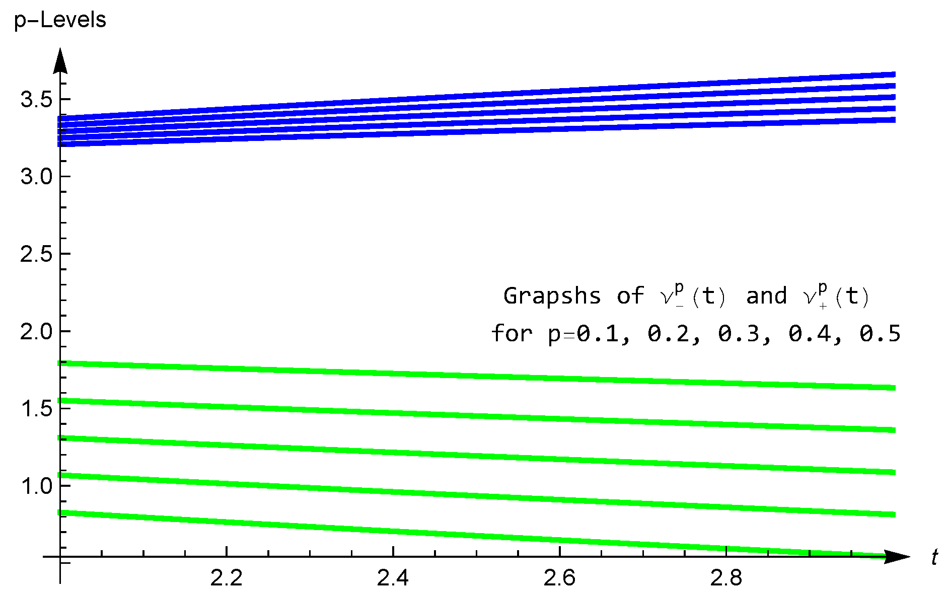
Example 1.

Consider the fuzzy number-valued mapping ν$:\left[2,3\right]\to {\mathbb{R}}_{\mathcal{F}}$ defined by

$$\nu \left(t\right)\left(\theta \right)=\left\{\begin{array}{cc}{\displaystyle \frac{\theta -2+t^{\frac{1}{2}}}{1-t^{\frac{1}{2}}}},& \theta \in \left[2-t^{{\displaystyle \frac{1}{2}}},3\right]\\ & \\ {\displaystyle \frac{2+t^{\frac{1}{2}}-\theta }{t^{\frac{1}{2}}-1}},& \theta \in \left(3,2+t^{{\displaystyle \frac{1}{2}}}\right]\\ & \\ 0,& otherwise.\end{array}\right.$$

Then, for each $p\in \left[0,1\right]$, we have

$${\nu }^p\left(t\right)=\left[\left(1-p\right)\left(2-t^{{\displaystyle \frac{1}{2}}}\right)+3p,\left(1-p\right)\left(2+t^{{\displaystyle \frac{1}{2}}}\right)+3p\right]=\left[{\nu }_{-}^p\left(t\right),{\nu }_{+}^p\left(t\right)\right].$$

We also define a mapping $\phi :\left[2,3\right]\to {\mathbb{R}}^{+}$ by $\phi \left(t\right)=t^2$. Then, according to the metric $\mathcal{D}:{\mathbb{R}}_{\mathcal{F}}\times {\mathbb{R}}_{\mathcal{F}}⟶{\mathbb{R}}^{+}\cup \left\{0\right\}$ as defined in the beginning of Section 2 with $\lambda ={\displaystyle \frac{5}{2}}\in \left[2,3\right]$ and $w=4,r={\displaystyle \frac{4}{3}}$, then the inequality (14) takes the following form:

$$\begin{array}{c}\mathcal{D}\left(\left({\int }_{{\displaystyle \frac{5}{2}}}^3\phi \left(s\right)ds\right)\odot \nu \left(3\right){\ominus }_{\phi H}\left(-{\int }_2^{{\displaystyle \frac{5}{2}}}\phi \left(s\right)ds\right)\right.\left.\odot \nu \left(2\right){\ominus }_{\phi H}{\int }_2^3\phi \left(t\right)\odot \nu \left(t\right)dt,\tilde{0}\right)\hfill \\ \hfill \le B\left(\phi ,\nu ,{\displaystyle \frac{5}{2}}\right).\end{array}$$

(48)

We now calculate the left hand side in (48) as follows:

$$\begin{array}{c}\mathcal{D}\left(\left({\int }_{{\displaystyle \frac{5}{2}}}^3\phi \left(s\right)ds\right)\odot \nu \left(3\right){\ominus }_{\phi H}\left(-{\int }_2^{{\displaystyle \frac{5}{2}}}\phi \left(s\right)ds\right)\odot \nu \left(2\right){\ominus }_{\phi H}{\int }_2^3\phi \left(t\right)\odot \nu \left(t\right)dt,\tilde{0}\right)\hfill \\ =\mathcal{D}\left(\left({\int }_{{\displaystyle \frac{5}{2}}}^3{s}^{2}ds\right)\odot \nu \left(3\right)-\left(-{\int }_2^{{\displaystyle \frac{5}{2}}}{s}^{2}ds\right)\odot \nu \left(2\right)-{\int }_2^3{t}^2\odot \nu \left(t\right)dt,\tilde{0}\right)\\ =\left(2+3^{{\displaystyle \frac{1}{2}}}\right)\left({\int }_{{\displaystyle \frac{5}{2}}}^3{s}^{2}ds\right)+\left(2+2^{{\displaystyle \frac{1}{2}}}\right)\left({\int }_2^{{\displaystyle \frac{5}{2}}}{s}^{2}ds\right)-{\int }_2^3{t}^2\left(2+t^{{\displaystyle \frac{1}{2}}}\right)dt\\ \hfill ={\displaystyle \frac{61}{24}}\left(\sqrt{2}+2\right)+{\displaystyle \frac{91}{24}}\left(\sqrt{3}+2\right)+{\displaystyle \frac{1}{168}}\left(384\sqrt{2}-375\sqrt{10}-854\right)=0.0327721.\end{array}$$

where

$$\begin{array}{c}\hfill B\left(\phi ,\nu ,{\displaystyle \frac{5}{2}}\right):={\int }_{{\displaystyle \frac{5}{2}}}^3\left({\int }_t^3\phi \left(s\right)ds\right)\mathcal{D}\left({\nu }_{\phi H}^{\prime }\left(t\right),\tilde{0}\right)dt+{\int }_2^{{\displaystyle \frac{5}{2}}}\left({\int }_2^t\phi \left(s\right)ds\right)\mathcal{D}\left({\nu }_{\phi H}^{\prime }\left(t\right),\tilde{0}\right)dt.\end{array}$$

Now, we calculate the bounds for $B\left(\phi ,\nu ,{\displaystyle \frac{5}{2}}\right)$ as follows:

$$B\left(\phi ,\nu ,{\displaystyle \frac{5}{2}}\right)\le \left\{\begin{array}{c}{\int }_{{\displaystyle \frac{5}{2}}}^3{s}^{2}ds{\int }_{{\displaystyle \frac{5}{2}}}^3{\displaystyle \frac{1}{2\sqrt{t}}}dt+{\int }_2^{{\displaystyle \frac{5}{2}}}{s}^{2}ds{\int }_2^{{\displaystyle \frac{5}{2}}}{\displaystyle \frac{1}{2\sqrt{t}}}dt\hfill \\ \\ {\left[{\int }_{{\displaystyle \frac{5}{2}}}^3\left({\int }_{{\displaystyle \frac{5}{2}}}^t{s}^{8}ds\right)dt\right]}^{{\displaystyle \frac{1}{4}}}{\left({\int }_{{\displaystyle \frac{5}{2}}}^3{\left[{\displaystyle \frac{1}{2\sqrt{t}}}\right]}^{{\displaystyle \frac{4}{3}}}dt\right)}^{{\displaystyle \frac{3}{4}}}\hfill \\ +{\left[{\int }_2^{{\displaystyle \frac{5}{2}}}\left({\int }_t^{{\displaystyle \frac{5}{2}}}{s}^{8}ds\right)dt\right]}^{{\displaystyle \frac{1}{4}}}{\left({\int }_2^{{\displaystyle \frac{5}{2}}}{\left[{\displaystyle \frac{1}{2\sqrt{t}}}\right]}^{{\displaystyle \frac{4}{3}}}dt\right)}^{{\displaystyle \frac{3}{4}}},\hfill \\ \\ {\displaystyle \frac{1}{2}}\sqrt{{\displaystyle \frac{2}{5}}}{\int }_{{\displaystyle \frac{5}{2}}}^3\left({\int }_t^3{s}^{2}ds\right)dt+{\displaystyle \frac{1}{2\sqrt{2}}}{\int }_2^{{\displaystyle \frac{5}{2}}}\left({\int }_2^t{s}^{2}ds\right)dt.\hfill \end{array}\right.$$

We use the software Mathematica to evaluate the above integrals as follows:

$$\begin{array}{c}{\int }_{{\displaystyle \frac{5}{2}}}^3{s}^{2}ds{\int }_{{\displaystyle \frac{5}{2}}}^3{\displaystyle \frac{1}{2\sqrt{t}}}dt+{\int }_2^{{\displaystyle \frac{5}{2}}}{s}^{2}ds{\int }_2^{{\displaystyle \frac{5}{2}}}{\displaystyle \frac{1}{2\sqrt{t}}}dt\hfill \\ \hfill \hspace{1em}\hspace{1em}\hspace{1em}\hspace{1em}\hspace{1em}\hspace{1em}\hspace{1em}\hspace{1em}\hspace{1em}\hspace{1em}\hspace{1em}\hspace{1em}\hspace{1em}={\displaystyle \frac{91}{24}}\left(\sqrt{3}-\sqrt{{\displaystyle \frac{5}{2}}}\right)+{\displaystyle \frac{61\left(\sqrt{5}-2\right)}{24\sqrt{2}}}=0.996476,\end{array}$$

$$\begin{array}{c}{\left[{\int }_{{\displaystyle \frac{5}{2}}}^3\left({\int }_2^t{s}^{8}ds\right)dt\right]}^{{\displaystyle \frac{1}{4}}}{\left({\int }_{{\displaystyle \frac{5}{2}}}^3{\left[{\displaystyle \frac{1}{2\sqrt{t}}}\right]}^{{\displaystyle \frac{4}{3}}}dt\right)}^{{\displaystyle \frac{3}{4}}}\hfill \\ +{\left[{\int }_2^{{\displaystyle \frac{5}{2}}}\left({\int }_t^3{s}^{8}ds\right)dt\right]}^{{\displaystyle \frac{1}{4}}}{\left({\int }_2^{{\displaystyle \frac{5}{2}}}{\left[{\displaystyle \frac{1}{2\sqrt{t}}}\right]}^{{\displaystyle \frac{4}{3}}}dt\right)}^{{\displaystyle \frac{3}{4}}}\\ \hfill ={\displaystyle \frac{1}{16}}{\left(\sqrt[3]{6}-\sqrt[3]{5}\right)}^{3/4}\sqrt[4]{{\displaystyle \frac{144,237,333}{5}}}+{\displaystyle \frac{1}{16}}\sqrt[4]{{\displaystyle \frac{10,228,879}{10}}}{\left(3\left(\sqrt[3]{10}-2\right)\right)}^{3/4}=1.97398\end{array}$$

and

$$\begin{array}{c}\hfill {\displaystyle \frac{1}{2}}\sqrt{{\displaystyle \frac{2}{5}}}{\int }_{{\displaystyle \frac{5}{2}}}^3\left({\int }_t^3{s}^{2}ds\right)dt+{\displaystyle \frac{1}{2\sqrt{2}}}{\int }_2^{{\displaystyle \frac{5}{2}}}\left({\int }_2^t{s}^{2}ds\right)dt={\displaystyle \frac{83}{192}}\sqrt{{\displaystyle \frac{5}{2}}}+{\displaystyle \frac{165}{128\sqrt{2}}}=1.59502.\end{array}$$

Hence, it can be observed from the above calculations of that the inequality (14) of Theorem 16 is valid for the above choices of functions over the interval $[2,3]$ Figure 1.

4. Concluding Remarks

In the last forty years, there has been significant growth in the field of mathematical inequalities. Many researchers have published a plethora of articles using innovative approaches. Within the extensive literature on mathematical inequalities, trapezoidal-type inequalities stand out as important. These inequalities are utilized to estimate the absolute deviation of the average value of a function’s values at the end points of a closed interval of the real line from its integral mean.

Mathematicians have established various generalizations of trapezoidal-type inequalities, such as those for functions of bounded variation, Lipschitzian mappings, absolutely continuous functions, operator convex functions, and those involving two functions with values in Banach spaces. One of the notable studies on the generalizations of trapezoidal-type inequalities is highlighted in the paper [9].

In the present study, a more general result of the trapezoidal-type in the fuzzy context is proven, which generalizes not only the results from [9] but also extends the results from [1,2,4,7,8]. In order to obtain the results, a number of novel results from the theory of calculus of fuzzy number-valued functions were used. An identity has been proven by using the integration by parts, the properties of space of fuzzy numbers, and by employing the Hölder inequality to prove several new and novel inequalities of the trapezoidal-type for functions that have values in the space of fuzzy numbers. A numerical example is given to exhibit the validity of the obtained results. The results of this study can be a good source to obtain more new results for the researchers working in the field of mathematical inequalities in fuzzy number-valued calculus.

References

1. Cerone, P.; Dragomir, S.S.; Pearce, C.E.M. A generalised trapezoid inequality for functions of bounded variation. Turk. J. Math. 2000, 24, 147–163. [Google Scholar]
2. Dragomir, S.S. On the trapezoid quadrature formula for Lipschitzian mappings and applications. Tamkang J. Math. 1999, 30, 133–138. [Google Scholar] [CrossRef]
3. Cerone, P.; Dragomir, S.S. Trapezoidal-type rules from an inequalities point of view. In Handbook of Analytic-Computational Methods in Applied Mathematics; Anastassiou, G.A., Ed.; Chapman & Hall/CRC Press: New York, NY, USA, 2000; pp. 65–134. [Google Scholar]
4. Dragomir, S.S. Reverses of operator Féjer’s inequalities. Tokyo J. Math. 2021, 44, 351–366. [Google Scholar] [CrossRef]
5. Dragomir, S.S. Operator Inequalities of Ostrowski and Trapezoidal Type. In Springer Briefs in Mathematics; Springer: New York, NY, USA, 2012; p. x+112. ISBN 978-1-4614-1778-1. [Google Scholar]
6. Dragomir, S.S. Riemann–Stieltjes Integral Inequalities for Complex Functions Defined on Unit Circle with Applications to Unitary Operators in Hilbert Spaces; CRC Press: Boca Raton, FL, USA, 2019; 160p, ISBN 9780367337100. [Google Scholar]
7. Dragomir, S.S. Generalised trapezoid-type inequalities for complex functions defined on unit circle with applications for unitary operators in Hilbert spaces. Mediterr. J. Math. 2015, 12, 573–591. [Google Scholar] [CrossRef]
8. Dragomir, S.S. Trapezoid type inequalities for complex functions defined on the unit circle with applications for unitary operators in Hilbert spaces. Georgian Math. J. 2016, 23, 199–210. [Google Scholar] [CrossRef]
9. Dragomir, S.S. Generalized trapezoid type inequalities for functions with values in Banach spaces. J. Iran. Math. Soc. 2021, 2, 17–38. [Google Scholar]
10. Barnett, N.S.; Buşe, C.; Cerone, P.; Dragomir, S.S. On weighted Ostrowski type inequalities for operators and vector-valued functions. J. Inequal. Pure Appl. Math. 2002, 3, 12. [Google Scholar]
11. Latif, M.A. More general Ostrowski type inequalities in the fuzzy context. Mathematics 2024, 12, 500. [Google Scholar] [CrossRef]
12. Anastassiou, G.A. Ostrowski type inequalities. Proc. Am. Math. Soc. 1995, 123, 3775–3791. [Google Scholar] [CrossRef]
13. Ahmadini, A.A.H.; Afzal, W.; Abbas, M.; Aly, E.S. Weighted Fejér, Hermite–Hadamard, and Trapezium-Type Inequalities for (h1, h2)–Godunova–Levin Preinvex Function with Applications and Two Open Problems. Mathematics 2024, 12, 382. [Google Scholar] [CrossRef]
14. Anastassiou, G.A. Fuzzy Ostrowski type inequalities. J. Comput. Appl. Math. 2003, 22, 279–292. [Google Scholar] [CrossRef]
15. Anastassiou, G.A. Ostrowski and Landau inequalities for Banach space valued functions. Math. Comput. Model. 2012, 55, 312–329. [Google Scholar] [CrossRef]
16. Hezenci, F.; Budak, H. Novel results on trapezoid-type inequalities for conformable fractional integrals. Turk. J. Math. 2023, 47, 425–438. [Google Scholar] [CrossRef]
17. Dragomir, S.S. A refinement of Ostrowski’s inequality for absolutely continuous functions whose derivatives belong to L and applications. Lib. Math. 2002, 22, 49–63. [Google Scholar]
18. Latif, M.A.; Almutairi, O.B. Ostrowski-Type Inequalities for Functions of Two Variables in Banach Spaces. Mathematics 2024, 12, 2748. [Google Scholar] [CrossRef]
19. Niu, Y.; Ali, R.S.; Talib, N.; Mubeen, S.; Rahman, G.; Yildiz, C.; Awwad, F.A.; Ismail, E.A.A. Exploring Advanced Versions of Hermite-Hadamard and Trapezoid-Type Inequalities by Implementation of Fuzzy Interval-Valued Functions. J. Funct. Spaces 2024, 2024, 1988187. [Google Scholar] [CrossRef]
20. Stojiljković, V.; Mirkov, N.; Radenović, S. Variations in the Tensorial Trapezoid Type Inequalities for Convex Functions of Self-Adjoint Operators in Hilbert Spaces. Symmetry 2024, 16, 121. [Google Scholar] [CrossRef]
21. Wu, C.; Gong, Z. On Henstock integral of fuzzy number valued functions (I). Fuzzy Sets Syst. 2001, 120, 523–532. [Google Scholar] [CrossRef]
22. Congxin, W.; Ming, M. On embedding problem of fuzzy number space: Part 3. Fuzzy Sets Syst. 1992, 16, 281–286. [Google Scholar] [CrossRef]
23. Anastassiou, G.A.; Gal, S. On a fuzzy trigonometric approximation theorem of Weierstrass-type. J. Fuzzy Math. 2001, 9, 701–708. [Google Scholar]
24. Kaleva, O.; Seikkala, S. On fuzzy metric spaces. Fuzzy Sets Syst. 1984, 12, 215–229. [Google Scholar] [CrossRef]
25. Stefanini, L. A generalization of Hukuhara difference and division for interval and fuzzy arithmetic. Fuzzy Sets Syst. 2010, 161, 1564–1584. [Google Scholar] [CrossRef]
26. Bede, B.; Stefanini, L. Generalized differentiability of fuzzy-valued functions. Fuzzy Sets Syst. 2013, 230, 119–141. [Google Scholar] [CrossRef]
27. Stefanini, L.; Bede, B. Generalized Hukuhara differentiability of interval-valued functions and interval differential equations. Nonlinear Anal. 2009, 71, 1311–1328. [Google Scholar] [CrossRef]
28. Anastassiou, G.A. Fuzzy Mathematics: Approximation Theory. In Studies in Fuzziness and Soft Computing; Springer: Berlin/Heidelberg, Germany, 2010. [Google Scholar]
29. Gouyandeh, Z.; Allahviranloo, T.; Abbasbandy, S.; Armand, A. A fuzzy solution of heat equation under generalized Hukuhara differentiability by fuzzy Fourier transform. Fuzzy Sets Syst. 2017, 309, 81–97. [Google Scholar] [CrossRef]
30. Kaleva, O. Fuzzy differential equations. Fuzzy Sets Syst. 1987, 24, 301–317. [Google Scholar] [CrossRef]
31. Anastassiou, G.A. Rate of convergence of Fuzzy neural network operators, univariate case. J. Fuzzy Math. 2002, 755–780. [Google Scholar]
32. Anastassiou, G.A. On H-fuzzy differentiation. Math. Balk. 2002, 16, 153–193. [Google Scholar]
33. Armand, A.; Allahviranloo, T.; Gouyandeh, Z. Some fundamental results on fuzzy calculus. Iran. J. Fuzzy Syst. 2018, 15, 27–46. [Google Scholar]
34. Ostrowski, A. Über die Absolutabweichung einer differentiebaren Funktion von ihrem Integralmittelwert. Comment. Math. Helv. 1937, 10, 226–227. [Google Scholar] [CrossRef]
35. Matić, M.; Barnes, E.S.; Marsh, D.C.B.; Radok, J.R.M. Elementary Inequalities; P. Noordhoff Ltd.: Groningen, The Netherlands, 1964. [Google Scholar]
Figure 1. Graphs of p-levels of v p ( t ) are shown in green and those of v + p ( t ) are shown in blue.
Mathematics 12 03112 g001
Disclaimer/Publisher’s Note: The statements, opinions and data contained in all publications are solely those of the individual author(s) and contributor(s) and not of MDPI and/or the editor(s). MDPI and/or the editor(s) disclaim responsibility for any injury to people or property resulting from any ideas, methods, instructions or products referred to in the content.