Characterization Model Research on Deformation of Arch Dam Based on Correlation Analysis Using Monitoring Data

Abstract

Deformation is the most direct indicator of structural state changes in arch dams. Therefore, numerous deformation monitoring points are typically arranged on arch dams to obtain deformation data from each point. Considering the complex relationships between the deformation at each monitoring point, this study focuses on the internal structural relationships and information fusion within the dam. The Pearson correlation coefficient is used as a similarity index to determine significant linear correlations between the measuring points. Ward’s cluster analysis method is then applied to group these points based on their similarities. To identify measuring points with strong nonlinear correlations, the Maximum Information Coefficient (MIC) method is employed. By integrating these linear and nonlinear correlations, a model is constructed to characterize the deformation at specific measurement points using data from strongly correlated points. The effectiveness of this model is verified through a concrete engineering case study, offering a novel approach for analyzing arch dam deformations.

1. Introduction

In the field of dam safety monitoring, numerous scholars have conducted extensive analysis and research on arch dam deformation monitoring data, leading to a wealth of valuable findings. However, most existing methods primarily focus on the influence of load on the deformability of arch dams, aiming to establish deformability representation models. These models are crucial for accurately analyzing and monitoring arch dam deformability, enabling operational management personnel to make informed judgments about dam safety.

Current methods for representing arch dam deformability typically model and analyze the deformability of monitoring points based on factors such as water pressure, temperature, and aging. These approaches include statistical models, deterministic models, and mixed models, all of which are widely used in engineering practice. For instance, Li et al. [1] established a new approach for the prediction of effect quantity through increasing sample information based on discrete and regression analysis of two-dimensional normal information diffusion. Chen et al. [2] developed a multi-objective prediction method that has been successfully applied to deformation prediction and anomaly detection in arch dams. Similarly, Kang et al. [3] proposed a displacement change analysis model for concrete gravity dams based on Gaussian process regression, effectively analyzing dam deformation trends. Building on previous research, Li and Xu [4,5,6], among others, proposed a partial least squares regression statistical model for dam deformation analysis, aimed at overcoming the limitations of the least squares regression method. Yang, Deng, and Wang [7,8,9] replaced stepwise linear regression with partial regression models, achieving better deformation representation for dam monitoring points. In recent years, significant progress has also been made in deterministic modeling. For example, Li et al. [10] proposed a method for determining the temperature field of arch dams by correlating dam temperature boundaries with air and water temperatures, subsequently establishing a deterministic displacement model for arch dams. Shen et al. [11] used a deterministic model based on a viscoelastic constitutive framework to monitor deformation during the construction of the Three Gorges Dam, estimating the viscoelastic deformation of the dam body and foundation, thereby providing a theoretical basis for ensuring safety during construction. Regarding mixed models, additionally, Li et al. [12] used the finite element method to calculate theoretical water pressure displacement for two dam sections under various conditions, characterizing dam deformation at different water levels and exploring the complementary use of theoretical calculations and statistical analysis.

In recent years, the rapid advancement of data mining and artificial intelligence technologies has led to the introduction of contemporary mathematical theories and swarm intelligence algorithms into the construction of dam deformation analysis models [13,14,15,16]. This integration has yielded several valuable research outcomes. Su et al. [17] proposed an optimization method for support vector machine parameters and input vectors, which enhanced the efficiency of establishing dam safety monitoring models and dynamically described the mapping relationship between dam structural behavior and its influencing factors. Gabriella et al. [18] developed three multi-objective support vector regression models, which were then used to construct deformability state representation models for dams. Wei et al. [19] introduced a concrete dam deformation prediction model based on the Chicken Swarm Optimization (CSO) Support Vector Machine (RVM), which effectively addressed the complex nonlinear relationships between dam deformation and environmental factors, improving prediction accuracy. Li et al. [20] developed a dam deformation prediction model that uses an improved particle swarm optimization algorithm to select the optimal parameters for an Extreme Learning Machine (ELM-IPSO), aiming to overcome the slow convergence and overfitting issues of traditional neural network models. Zhou et al. [21] proposed a dam deformation representation and prediction model based on Complete Ensemble Empirical Mode Decomposition with Adaptive Noise (CEEMDAN), Phase Space Reconstruction (PSR), and Kernel Extreme Learning Machine (KELM). This model improved prediction accuracy by addressing the nonlinear and non-stationary characteristics of dam deformation monitoring sequences. Guo et al. [22] established a concrete dam deformation prediction model using deformation monitoring data from concrete dam prototypes, leveraging the open-source deep learning framework TensorFlow, thereby providing a highly accurate means of predicting dam behavior.

The aforementioned research primarily focuses on the impact of load on the deformation behavior of arch dams, leading to the development of deformation state representation and early warning models. However, arch dams are highly nonlinear structures, and their deformation behavior is not only influenced by loads but also by complex correlations between deformation at different measurement points within the dam. Therefore, future research should further investigate the deformation representation model of each measurement point from the perspective of internal correlation and information fusion within the dam structure. This approach would better capture the interrelated effects across different parts of the dam and provide a new technical means for the deformation safety monitoring of arch dams.

2. Analysis of Deformation Correlation of Each Measurement Point of Arch Dam

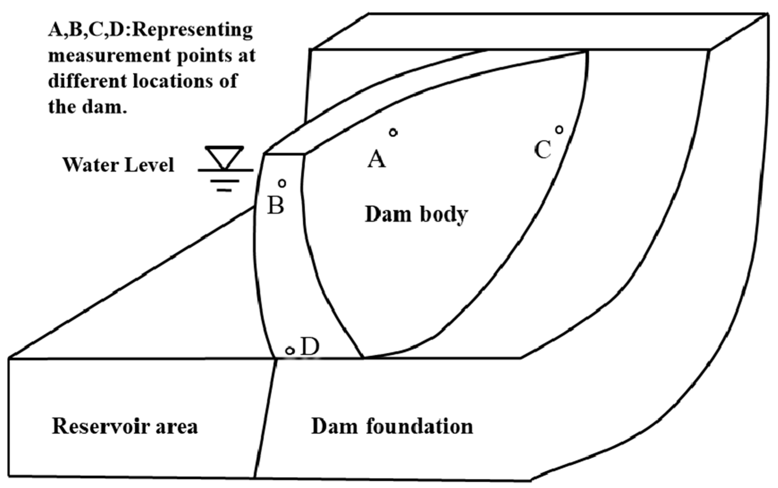
In practical engineering (Figure 1), the deformations observed at measurement points A, B, C, and D are primarily influenced by common factors such as hydraulic pressure, temperature, and aging. However, the deformation patterns at points C and D, located near the dam foundation and bank slope, differ significantly from those at points A and B, which are situated near the dam crest. This variation is closely linked to the combined effects of structural constraints, material properties, and environmental conditions specific to different regions of the dam, resulting in distinct deformation behaviors. When the deformation analysis model fails to account for these complex, unmonitored, and unquantifiable factors, parameter heterogeneity arises. Although traditional deformation models can capture the primary influencing factors through independent variables, they often overlook the unique deformation characteristics at different measurement points caused by these complex influences. Given the intricate nature of arch dam structures, the deformations at various measurement points are interrelated. Therefore, by analyzing the internal correlations within the arch dam structure and integrating prototype monitoring data, the deformation behavior of the dam can be assessed using information fusion techniques. This approach helps to mitigate the impact of specific, non-monitored environmental factors on the deformations at different measurement points.

In the following, the deformation of any two measurement points of the arch dam will be correlation analyzed through linear correlation coefficient and nonlinear correlation coefficient, and the deformation measurement points with similar characteristics will be analyzed by clustering.

2.1. Method to Identify Measurement Points with Strong Linear Correlation

To explore the correlation between deformation of two measurement points from the perspective of correlation, the Pearson correlation coefficient is used as the similarity index for cluster analysis. Measurement points within the same cluster exhibit strong linear correlation, while those in different clusters represent weak linear correlation. The expression for the Pearson correlation coefficient is [23]:

$$r_{ij}^{\mathrm{P}}={\displaystyle \frac{{\displaystyle \sum _{t=1}^T({\delta }_{it}-{\overline{\delta }}_i)({\delta }_{jt}-{\overline{\delta }}_j)}}{\sqrt{{\displaystyle \sum _{t=1}^T{({\delta }_{it}-{\overline{\delta }}_i)}^2{\displaystyle \sum _{t=1}^T{({\delta }_{jt}-{\overline{\delta }}_j)}^2}}}}}$$

(1)

where T is number of time slices; $\left\{{\delta }_{it}\right\}(t=1,2,3,\cdots ,T)$ and $\left\{{\delta }_{jt}\right\}(t=1,2,3,\cdots ,T)$ are the deformation time series of the measurement points $i$ and $j$, respectively; ${\overline{\delta }}_i$ is the mean of $\left\{{\delta }_{it}\right\}(t=1,2,3,\cdots ,T)$; ${\overline{\delta }}_j$ is the mean of $\left\{{\delta }_{jt}\right\}(t=1,2,3,\cdots ,T)$.

The basic principle of the deformation cluster analysis based on the Ward method [24] for arch dam measurement points is as follows:

Assume that $N$ deformation measurement points of the arch dam are divided into $k$ clusters, denoted as $G_1,G_2,\cdots ,G_k$. $N_l$ represents the number of deformation measurement points in the $G_l$ cluster, $X_{il}$ represents the similar index value of the measurement points $i$ ($i=1,2,\cdots ,N_l$) in the $G_l$ cluster (the paper refers to the deformation correlation coefficient), and ${\overline{X}}_l$ is the center of the index of $G_l$. Then, $W_l$ (the sum of squares of deviations of the measurement points in the $G_l$) can be expressed as

$$W_l={\displaystyle \sum _{i=1}^{N_l}{(X_{il}-{\overline{X}}_l)}^2}$$

(2)

The total sum of squares of the deviations of $k$ clusters of the arch dam is

$$W={\displaystyle \sum _{l=1}^k{W}_l}$$

(3)

where ${\overline{X}}_l$ is the average value of the correlation coefficient of the points in the $G_l$.

When $k$ is determined, the classification which can be selected to make $W$ minute is the optimal classification. However, so far as practical engineering, the number $k$ of clusters is unknown in advance. In view of this situation, the paper conducts research on a Threshold Method to determine the number of deformation clusters in an arch dam.

Assuming that the clustering process merges $n$ times in total, $S_l$ (the ratio of the similarity distance between the clusters of the $lth$ clustering and the last clustering) is calculated, that is

$$S_l={\displaystyle \frac{D_l}{D_{n-1}}}$$

(4)

where $D_l$ is the global sum of squares of total deviations in the $lth$ partition; $D_{n-1}$ is the global sum of squares of total deviations in the last partition.

$S_l$ ($i=l-1,l,l+1$) can be calculated by Equation (4). When the difference between $S_i$ and $S_{l+1}$ is small while the difference between $S_i$ and $S_{i-1}$ is large, $D_l$ (the distance between the corresponding clusters) will be used as the threshold of the arch dam deformation clustering according to which the clustering cluster is determined.

As mentioned above, assuming that there are $N$ measurement points and $T$ monitoring moments in the arch dam, according to the deformation cor $S_{l+1}$ relation coefficient measure index of the arch dam and the Ward clustering method, the partition clustering process of the arch dam deformation is as follows:

Step 1: Standardize the deformation eigenvalues and calculate the correlation coefficient between $N$ measurement points according to the Equation (1) to obtain the initial matrix $D^{(0)}$.

Step 2: Initialize all measurement points form a cluster, the number of which $k=N$, $D^{(1)}=D^{(0)}$, for the $ith$ type $G_i=\left\{X_{(i)}\right\}(i=1,2,\cdots ,N)$, and then perform Step 3 and Step 4 for the measurement points $X_{(i)}(i=2,3,\cdots ,N)$.

Step 3: For the correlation coefficient matrix $D^{(i-1)}$ obtained in Step 2, the two most correlated classes are merged into a new class according to the classification criterion.

Step 4: Calculate the correlation distance between the new class and other classes to obtain a new distance matrix $D^{(i)}$. Repeat Step 3 and Step 4 until all measurement points are aggregated into one class.

Step 5: Determine the threshold of clustering $D_l$, and determine the number of classifications and the measurement points in each clustering partition.

Step 6: Investigate the spatial proximity characteristics of the clustering measurement points. For the discontinuous regions of the clustered measurement points, the clustering is continued according to their spatial coordinates until the final clustering result is determined.

After the above-mentioned cluster analysis, for the same cluster, the set of measurement points {$i$} where the deformation is linearly correlation at $t$ time and the $jth$ measurement point can be obtained.

2.2. Method to Identify Measurement Points with Strong Nonlinear Correlation

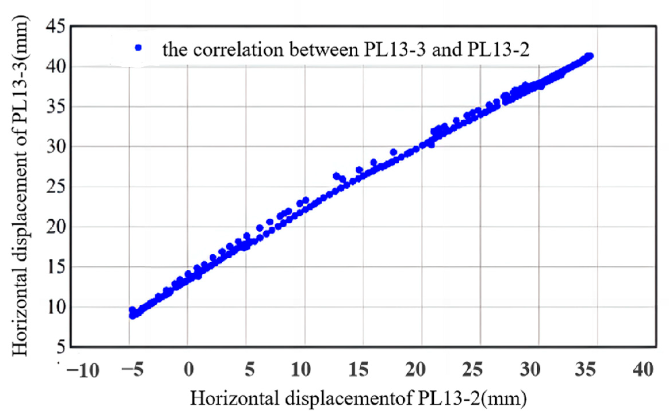
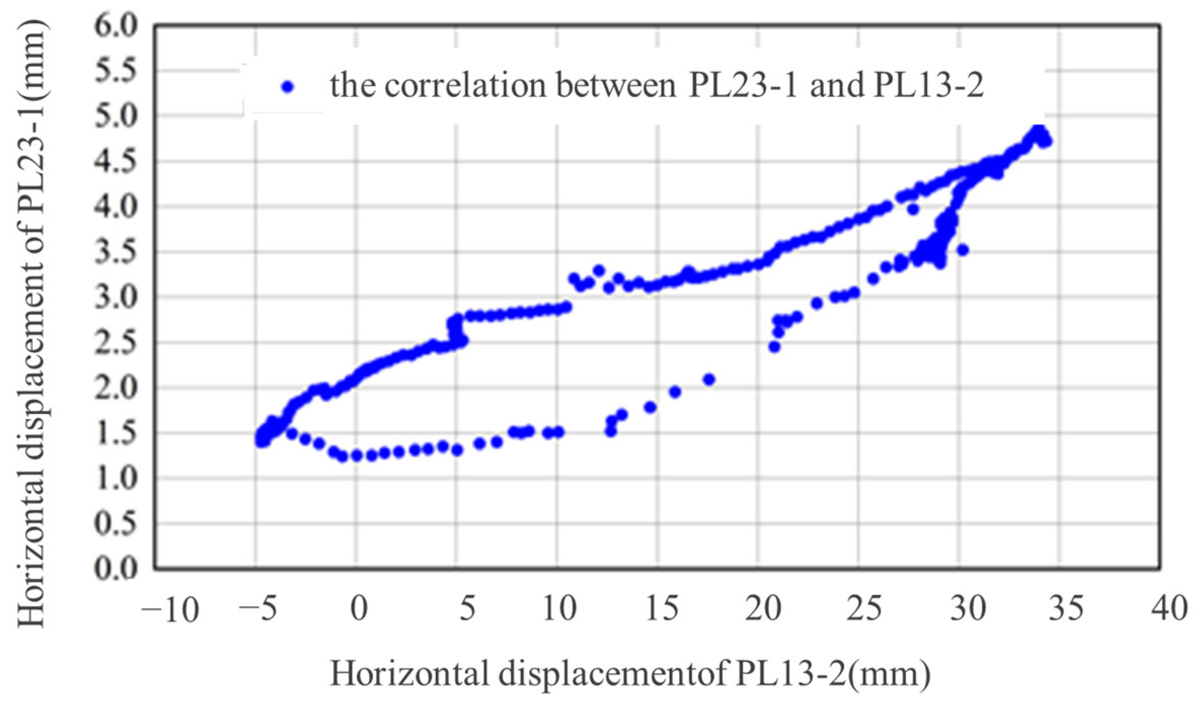
This paper performs cluster analysis using the correlation coefficient between the deformation sequences of measurement points as the similarity index, and then other measurement point sets {$i$} that are significantly linearly related to the deformation of the $jth$ measurement point are determined, that is to say, the deformation of the measurement points in the same cluster is with a significant linearity correlation. For different clusters, the linear correlation between the deformation of the two measurement points is weak, but there may be a certain nonlinear correlation. Therefore, the nonlinear correlation between the deformation of two measurement points in different clusters will be delved into below to determine the points that have a significant nonlinear correlation with the $jth$ measurement point.

The maximal information coefficient ($MIC$) is a correlation algorithm that evaluates the functional and statistical relationships between variables without making any assumptions about the data distribution. It was first proposed by Reshef et al. [25] to measure the degree of correlation between variables. Assume that the deformation sequences in T time at the two measurement points $X$,$Y$ of the arch dam are, respectively, $X=\left\{x_i,i=1,2,\cdots ,T\right\}$, $Y=\left\{y_i,i=1,2,\cdots ,T\right\}$, and their mutual information is defined as

$$I(X,Y)={\displaystyle \sum _{x\in X}{\displaystyle \sum _{y\in Y}p(x,y)}}\ln {\displaystyle \frac{p(x,y)}{p(x)p(y)}}$$

(5)

where $p(x,y)$ is the joint probability density of $X$ and $Y$; $p(x)$ and $p(y)$ are, respectively, the marginal probability density of $X$ and $Y$.

If the two constitute an ordered data set $D\left\{(x_i,y_i),i=1,2,\cdots ,T\right\}$, and the division G is defined as a grid of $x\ast y$ that the value range of the variable $X$ and $Y$ are divided into $x$ and $y$ segments respectively, the probability distribution $D{|}_G$ will be obtained when the variable values in D fall into the grid of G where the $x$ and $y$ are both positive integers. If the number of grid divisions is fixed, different mutual information values will be obtained by changing the grid division position. The maximum mutual information formula for D in this way is

$$I^{\ast }(D,x,y)=\max I(D{|}_G)$$

(6)

In order to facilitate the comparison between different dimensions, the maximum normalized values $I$ that are in the interval [0, 1] obtained under different divisions are formed into a characteristic matrix defined as $M{(D)}_{x,y}$, whose expression is

$$M{(D)}_{x,y}={\displaystyle \frac{I^{\ast }(D,x,y)}{{\ln }_{\min }\left\{x,y\right\}}}$$

(7)

Then the maximum information coefficient is

$$MIC(D)=\underset{xy<B(T)}{\max }\left\{M{(D)}_{x,y}\right\}$$

(8)

where $T$ is the time length of the deformation monitoring sequence, that is, the scale of the data set; $B(T)=T^{\alpha }$, setting the condition $xy<B(T)$, is meant to limit the grid size to divide the area, where it is recommended that the value $\alpha$ is 0.6 during practical application according to the literature [25]; namely, $B\left(n\right)=n^{0.6}$.

Therefore, the $MIC$ between the deformation sequences of the two measurement points of the arch dam is essentially a normalized maximum mutual information, and its value range is $\left[0,1\right]$. The correlation between the deformation sequences of the two measurement points of the arch dam can be excavated by using the $MIC$. In terms of nonlinear measurement between two variables by utilizing $MIC$, David N. Reshef et al. measured the nonlinear relationship between two variables by $MIC-R^2$, where $R^2$ is the coefficient of determination of a simple linear regression model between the two variables. When the $MIC$ is larger and $MIC-R^2>0.2$, it means that there is a strong nonlinear correlation between the two variables. This paper utilizes the hypothesis test method to determine the threshold value of the $MIC$, that is, assuming that the random variables of the deformation of the two measurement points of the arch dam in the null hypothesis analysis are independent, when the null hypothesis is rejected and $MIC-R^2>0.2$ under a given significance level, it indicates that there is a strong nonlinear correlation between the two variables at this time, indicating that there is a strong nonlinear correlation relationship between the monitoring sequences of the deformation of the two points in the arch dam.

Compared with other traditional nonlinear statistical correlation coefficients, the $MIC$ possesses two obvious advantages: generality and equitability. Generality refers to the case where there are enough deformation sequence data sets of two measurement points of the arch dam, different types of correlations between the two can be explored by the $MIC$, including functional relationships, such as parabolas, periodic functions, non-functional relationships, and even the hyperfunction of the synthesis of multiple functional relationships and so on; equitability refers to the case where the $MIC$ of different types of correlations with the same noise level do not differ significantly from one another. In summary, the calculation process of the $MIC$ model to determine the nonlinear correlation between the deformations of two measurement points of the arch dam is as follows:

(1)

Arrange $Y={\left\{y_i\right\}}_{i=1}^n$ (the deformation measured data sequence of the measurement points to be analyzed) and $X={\left\{x_i\right\}}_{i=1}^n$ (the deformation measured data sequence of other measurement points) in ascending order, then define the sorted $X$ as the abscissa axis to be divided into $s$ grids and the sorted $Y$ as the ordinate axis to be divided into $t$ grids. In this case, a grid $G$ is constituted by $s\times t$, at which point the points in the data set $D$ fall into $G$, and some of the cells are allowed to be empty sets.

(2)

Find the probability distribution function $D{|}_G$ of all cells in the divided grid $G$. Let $x_0^{\prime },x_1^{\prime },\cdots ,x_s^{\prime }$ be the $X$ axis data division point in the $D$, and $P=〈x_0^{\prime },x_1^{\prime },\cdots ,x_s^{\prime }〉$ be the $X$ axis data division in the $D$; let $y_0^{\prime },y_1^{\prime },\cdots y_t^{\prime }$ be the $Y$ axis data division point in the $D$, and $Q=〈y_0^{\prime },y_1^{\prime },\cdots y_t^{\prime }〉$ be the $Y$ axis data division in the $D$. Find the mutual information $I\left(P;Q\right)$, the maximum mutual information value $I^{\ast }\left(D,s,t\right)=\max I\left(D{|}_G\right)$ and the eigenmatrix value $M{\left(D\right)}_{s,t}$ in case of $D{|}_G$ under the condition of satisfying certain constraints.

(3)

Since different grids $G$ will form different $D{|}_G$, the globally optimal grid $s_0\times t_0$ is locked through an exhaustive search for the characteristic matrix, so as to determine the maximum information coefficient $MIC$ that characterizes the nonlinear correlation between the deformations of the two measurement points of the arch dam.

By utilizing the $MIC$ analysis of two measurement points in different clusters, the set $\left\{p\right\}$ of measurement points, which is nonlinearly related to the deformation of the $jth$ measurement point at $t$ time, can be obtained.

3. A Characterization Model for Deformation State of Arch Dams Based on Correlation Analysis

Section 2 of this paper explores methods for analyzing the correlation between deformations at various measurement points of the arch dam and identifies other measurement points that influence the deformation of the point under analysis. This section further investigates the deformation characterization model of each measurement point, focusing on the correlations between different parts of the dam. It also provides a foundation for developing a deformation monitoring model for each measurement point. The following section will discuss the construction of the deformation state representation model for individual measurement points of the arch dam.

Let the number of the deformation measurement points of the arch dam be $N$; the deformation monitoring value of the $j\mathit{th}$ measurement point at $t$ time is ${\delta }_{tj},(j=1,2,\cdots ,N;t=1,2,\cdots ,T)$, and its data matrix form is

$${\left[\begin{array}{cccc}{\delta }_{11}& {\delta }_{12}& \cdots & {\delta }_{1N}\\ {\delta }_{21}& {\delta }_{22}& \cdots & {\delta }_{2N}\\ ⋮& ⋮& \ddots & ⋮\\ {\delta }_{T1}& {\delta }_{22}& \cdots & {\delta }_{TN}\end{array}\right]}_{T\times N}$$

(9)

Equation (9) is a two-dimensional data set composed of multiple deformation monitoring data time series of the arch dam in the form of data. Considering that the arch dam is a whole structure, there is a correlation between the monitoring values of any two measurement points with time. Therefore, the deformation of any measurement point of the arch dam can be characterized by the deformation of other measurement points, namely

$${\delta }_{tj}=\beta {\delta }_{tl}+a_j+\epsilon$$

(10)

where $l\ne j,l,j=1,2,\cdots ,N;t=1,2,\cdots ,T$ $\mathrm{l}\ne \mathrm{j},\mathrm{l},\mathrm{j}=1,2,\cdots ,\mathrm{N};\mathrm{t}=1,2,\cdots ,\mathrm{T}$; ${\delta }_{tj}$ is the deformation monitoring value of the $jth$ measurement point at $t$ moment; ${\delta }_{tl}$ is the column matrix formed by the deformation of other measurement points when there is a significant relationship between the two measurement points; $\beta$ is the row matrix of the parameters to be estimated; ${\alpha }_j$ is a scalar constant representing the amount of deformation-specific effect produced by different parts of the arch dam under the condition of unique influencing factors; $\epsilon$ represents random error.

Equation (10) can be expressed as a function

$${\delta }_{tj}=g({\delta }_{ti})+f({\delta }_{tp})+a_j+\epsilon$$

(11)

where ${\delta }_{tj}$, ${\delta }_{ti}$, ${\delta }_{tp}$ are, respectively, the deformation of the measurement points $j,i,p$, at the $t$ moment; $g({\delta }_{ti})$ is the deformation value metric function of the measurement point $i$ that is significantly linearly related to the deformation of the measurement point $j$; $f({\delta }_{tp})$ is the deformation value metric function of the measurement point $p$ that is significantly nonlinearly related to the deformation of the measurement point $j$.

By performing cluster analysis on the deformation data of the arch dam monitoring points, other measurement points that are significantly related to the deformation of the measurement points to be analyzed are obtained. For the set of measurement points $\left\{i\right\}$ that are significantly linearly related to the measurement point $j$ to be analyzed, the deformation relationship can be expressed as

$${\delta }_{tj}~{\displaystyle \sum _{i=1}^n}{a}_i{\delta }_{ti}$$

(12)

where ${\delta }_{tj}$ is the deformation of the measurement point $j$ at $t$ time; ${\delta }_{ti}$ is the deformation of the measurement point set $\left\{i\right\}$ that is significantly linearly related to the measurement point $j$, $n$ is the number of measurement points that are significantly linearly related to the measurement point $j$; $a_i$ is the coefficient.

Based on $MIC$ nonlinear correlation analysis, other measurement point sets $\left\{p\right\}$ that are significantly nonlinearly related to the deformation of the measurement point $j$ to be analyzed are obtained, and the deformation relationship can be expressed as

$${\delta }_{tj}~{\displaystyle \sum _{p=1}^m}{\displaystyle \sum _{l=1}^{K_{\mathrm{C}}}{d}_p{\phi }_l\left({\delta }_{tp}\right)}$$

(13)

where ${\delta }_{tj}$ is the deformation of the measurement point $j$ at $t$ time; ${\delta }_{tp}$ is the deformation of the measurement point set $\left\{p\right\}$ that is significantly nonlinearly related to the measurement point $j$; $m$ is the number of measurement points that are significantly nonlinearly related to the measurement point $j$; $K_{\mathrm{C}}$ is the number of elementary function terms used to describe the nonlinear relationship between ${\delta }_{tj}$ and ${\delta }_{tp}$; ${\phi }_l\left({\delta }_{tp}\right)$ is the elementary function describing the nonlinear relationship between ${\delta }_{tj}$ and ${\delta }_{tp}$; $d_p$ is the coefficient.

In order to further determine the functional form that can characterize the nonlinear relationship between ${\delta }_{tj}$ and ${\delta }_{tp}$ based on the discrete deformation monitoring data of the arch dam, this section aims to find the optimal combination of all elementary functions that can be composed to represent the nonlinear relationship between ${\delta }_{tj}$ and ${\delta }_{tp}$ through the research on genetic algorithms by expressing the elementary function in the form of a gene string. The specific implementation process is as follows:

Assuming that ${\widehat{\delta }}_{tj}$ is the deformation of the measurement point $j$ at $t$ time fitted by the functional expression representing the nonlinear relationship, the total sum of squared errors at each data point is

$$\epsilon ={{\displaystyle \sum _{t=1}^T\left({\delta }_{tj}-{\widehat{\delta }}_{tj}\right)}}^2$$

(14)

It is illustrated that the smaller the function value, the more accurate the determined function expression. Considering that the genetic algorithm is usually used to solve the maximum value of the function, the objective function to find the combination of elementary functions that form the optimal function expression is

$$f_{\max }=C-\epsilon =C-{{\displaystyle \sum _{t=1}^T\left({\delta }_{tj}-{\widehat{\delta }}_{tj}\right)}}^2$$

(15)

where $C$ is a large enough positive number.

In order to determine various forms of function expressions, it is necessary to decompose the function expression into basic operation units consisting of constants, functions, powers, operators, and so on: $\left(A^{k_1}\right)\left({\phi }_l^{k_2}\left({\delta }_{tp}\right)\right)\left(+,-,\times ,÷\right)$, where ${\phi }_l\left({\delta }_{tp}\right)$ consists of commonly used elementary functions like $x,x^{-1},e^x,e^{-x},\sin x,\cos x,\tan x,\ln x$, etc.; $k_i=\left(1/5,1/3,1/2,1,2,3,4,5\right)$; $A$ is constant. The basic operation units are connected by operators. In order to perform genetic operations, the above relationship needs to be mapped into binary codes. The constants directly adopt binary numbers, with a total of eight bits. The first six bits are the integer part, and the last two bits are decimals; ${\phi }_l\left({\delta }_{tp}\right)$ and $k_i$ are represented by a three-bit binary code, and the operator is represented by a two-bit binary code. The coding scheme is shown in

Table 1. Elementary functions, powers, operators, and binary encoding schemes.

Binary Code	000	001	010	011	100	101	110	111	00	01	10	11
${\phi }_l\left({\delta }_{tp}\right)$	$x$	$x^{-1}$	$e^x$	$e^{-x}$	$\sin x$	$\cos x$	$\tan x$	$\ln x$
ki	1/5	1/3	1/2	1	2	3	4	5
operator									$+$	$-$	$\times$	$÷$

.

A set of binary strings, each with a length of 19, is constructed according to a specific order of operations. Each binary string is referred to as a single gene. This fundamental structure can be employed to combine various functional forms. In the context of a genetic algorithm, individuals are represented by single genes. When converting a binary string into a function, it is necessary to discard the last operator.

When utilizing the genetic algorithm to determine the nonlinear relationship function of deformation between the measurement points, it is necessary to first generate the initial population, generate a random number between one and six, determine $m$ (the number of single genes in the individual), and then randomly generate a binary length of $19\times m$ strings, forming a variable-length polygenic individual. By imitating the principle of survival of the fittest in nature, according to the elite strategy, the previous ($n=0.05\times pop\_size$, $pop\_size$ is the population size) $n$ individuals with the highest fitness function value in the current population are directly copied to the next generation. According to the principle that the larger the fitness function, the larger the probability of being selected, $0.95\times pop\_size$ individuals are generated as the parent to participate in the reproduction of the next generation of the population.

The crossover operation generates new offspring by exchanging segments of information between two parent individuals to create potentially superior offspring. Since the length of the gene in each individual is variable, the standard crossover method must be adapted. During the crossover operation, two parents are randomly selected based on the crossover rate. Each parent independently generates a crossover point, and the crossover is then performed. If the length of the remaining segment exceeds 10, it is randomly appended to form a single gene; otherwise, it is discarded. Mutation operations introduce further diversity into the population by randomly altering individual genes, thus helping to prevent premature convergence. In the mutation process, the algorithm selects an individual from the parent generation according to the mutation rate, and then randomly selects and mutates a gene within that individual.

Continue to run the above algorithm until the sum of squared errors of an individual calculated according to the formula is less than 0.05 or the evolutionary algebra reaches the set maximum value. Then, the function expression representing the nonlinear relationship between ${\delta }_{tj}$ and ${\delta }_{tp}$ can be determined.

So far, the characterization model between the deformation of the measurement point $j$ and the deformation of other measurement points at the $t$ moment is

$${\delta }_{tj}={\displaystyle \sum _{i=1}^n{\alpha }_i}{\delta }_{ti}+{\displaystyle \sum _{p=1}^m{\displaystyle \sum _{l=1}^{K_C}{d}_p{\phi }_l({\delta }_{tp})+{\beta }_j}}$$

(16)

where ${\delta }_{tj}$ is the deformation of the measurement point $j$ at $t$ time; ${\delta }_{ti}$ is the deformation of the measurement point that is linearly related to the deformation of the measurement point $j$, and $n$ is the number of measurement points; ${\delta }_{tp}$ is the deformation of the measurement point that is nonlinearly related to the deformation of the measurement point $j$, and $m$ is the number of measurement points; ${\alpha }_i$ and $d_p$ are coefficients; ${\beta }_j$ are scalar constants, which represent the specific deformation effects of different parts of the arch dam under the conditions of unique influencing factors.

Utilizing the research results in Section 2 of this paper, other deformation measurement points that are significantly linearly and nonlinearly related to the deformation of the measurement point $j$ are determined, and the deformation data expression of the single measurement point of the arch dam can be obtained by substituting them into the above formula. According to ${\delta }_{tj}$, ${\delta }_{ti}$, and ${\delta }_{tp}$, estimate the parameters ${\alpha }_i$, $d_p$, and ${\beta }_j$ by the least squares method, and finally determine the expression of the model.

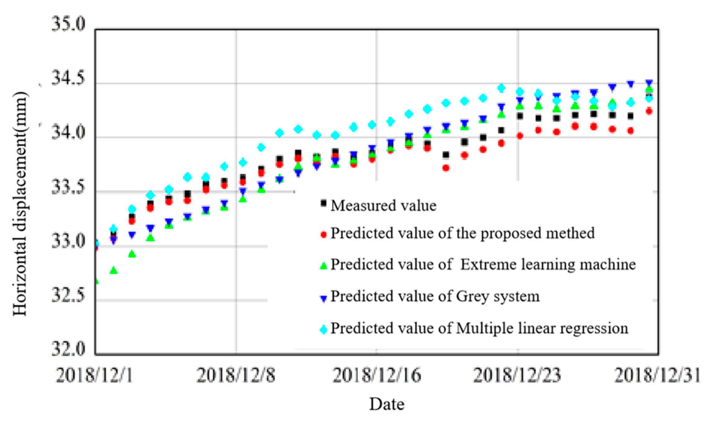
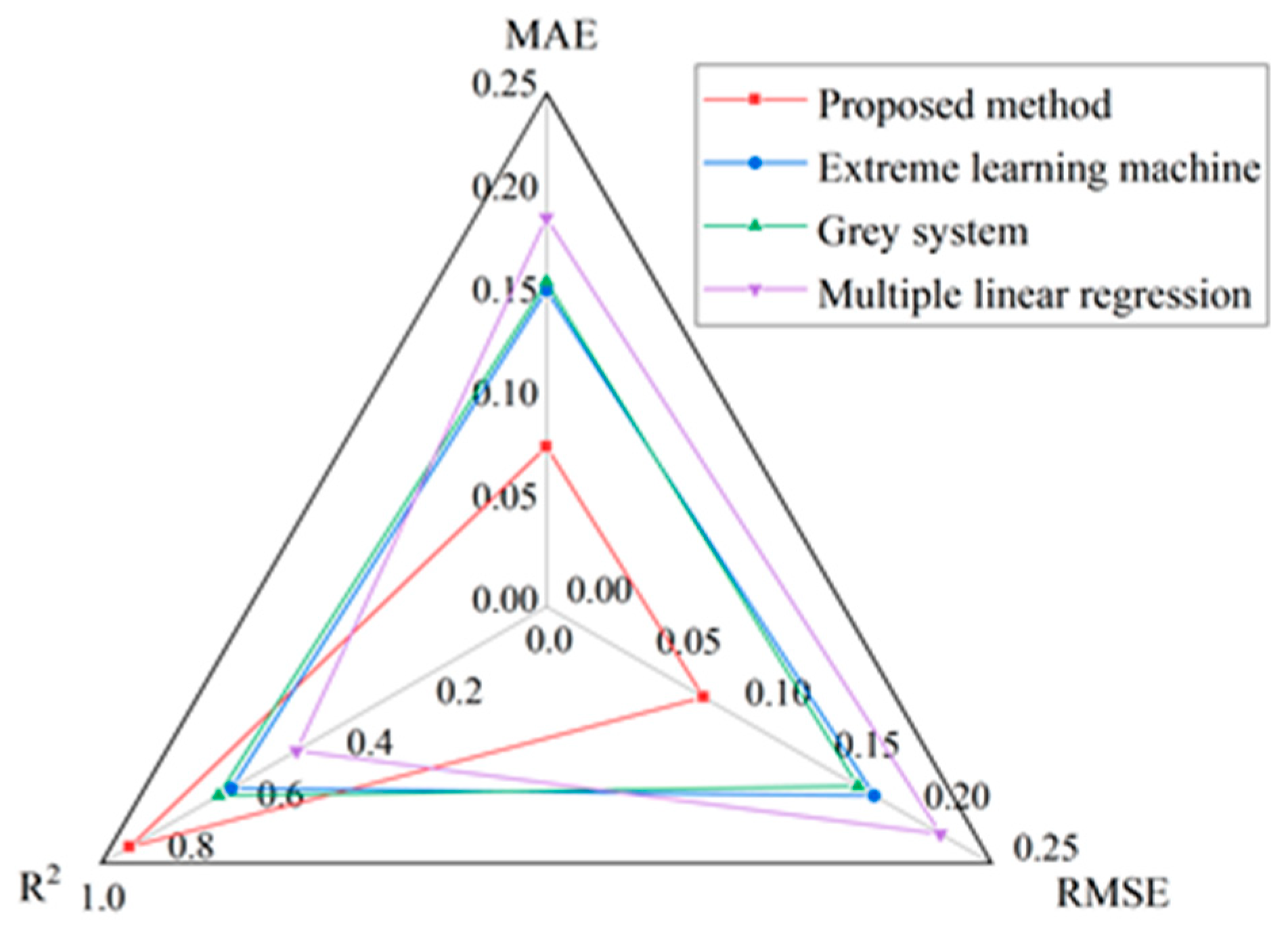
The developed model for characterizing the deformation state of the arch dam measurement points can be used for tracking and predicting the deformation behavior of these points.

4. The Example Analysis

4.1. Project Overview

In December 2013, the arch of the entire dam was sealed, as shown in Figure 2. To gain a detailed understanding of the deformation state of the dam, comprehensive monitoring was conducted using the deformation monitoring instruments installed throughout the dam. Horizontal deformation, including radial horizontal deformation and tangential horizontal deformation, was measured using the tension wire alignment method. The arrangement of measurement points is illustrated in Figure 3. A total of 34 measurement points were installed at various elevations: the top, 1829 m, 1778 m, 1730 m, 1664 m, and 1601 m across the 1#, 5#, 9#, 11#, 13#, 16#, 19#, and 23# dam sections. The deformation process for some measurement points is depicted in Figure 4.

4.2. Characterization Model of Deformability of Arch Dam

4.2.1. Determination of Significant Linear Correlation Measurement Points

To illustrate the correlation between deformations at each measurement point, the correlation coefficients between all pairs of the 34 measurement points were calculated. The results are displayed in Figure 5 drawn using the ggcorrplot package (Version 0.1.4.1). Figure 5 allows for a qualitative assessment of the correlations: ellipses that are more elongated indicate a stronger linear correlation between measurement points, while ellipses closer to a circular shape suggest a weaker linear correlation. As shown in Figure 5, there is a strong correlation between measurement points PL11-2 and PL11-5, whereas the correlation between measurement point PL1-1 and other measurement points is weak. To quantitatively assess the correlations, clustering analysis was performed on the deformation monitoring data from the 34 measurement points. The clustering results are presented in Figure 6 and

Table 2. Clustering and zoning results of horizontal deformation of an arch dam.

Altitude (m)	Section 1#	Section 5#	Section 9#	Section 11#	Section 13#	Section 16#	Section 19#	Section 23#
1885	Cluster 1# PL1-1	Cluster 2# PL5-1	Cluster 3# PL9-1	Cluster 3# PL11-1	Cluster 4# PL13-1	Cluster 5# PL16-1	Cluster 5# PL19-1	Cluster 6# PL23-1
1829		Cluster 2# PL5-2	Cluster 3# PL9-2	Cluster 4# PL11-2	Cluster 4# PL13-2	Cluster 4# PL16-2	Cluster 5# PL19-2
1778		Cluster 2# PL5-3	Cluster 3# PL9-3	Cluster 4# PL11-3	Cluster 4# PL13-3	Cluster 4# PL16-3	Cluster 5# PL19-3
1730		Cluster 2# PL5-4	Cluster 3# PL9-4	Cluster 4# PL11-4	Cluster 4# PL13-4	Cluster 4# PL16-4	Cluster 5# PL19-4
1664			Cluster 3# PL9-5	Cluster 4# PL11-5	Cluster 4# PL13-5	Cluster 4# PL16-5	Cluster 5# PL19-5
1601				Cluster 4# IP11-1	Cluster 4# IP13-2	Cluster 4# IP16-1

.

It can be seen from Figure 6 and Table 2 that the dam deformation is divided into six cluster zones, which may be affected by different landforms on the left and right banks, resulting in asymmetry between the left and right deformation zones, and the measurement points located in the same dam section are basically located in the same zone. In the first and sixth zones, there is only one measurement point: PL1-1 and PL23-1, respectively. The correlation between these two measurement points and other measurement points of the dam body is relatively weak, and their deformation is greatly affected by the mountain on both sides. The fourth zone contains 16 measurement points: PL11-2 to PL11-5, IP11-1, PL16-2 to PL16-5, IP16-1, PL13-1 to PL13-5, and IP131. For the deformation of all measurement points in the same partition with a strong correlation, take the fourth cluster partition, where measurement point PL13-2 is located as an example. The linear correlation coefficient of deformation between any two measurement points in this cluster partition is exhibited in

Table 3. Statistical table of correlation coefficient of each measurement point in 4# cluster.

Monitoring Point	PL11-2	PL11-3	PL11-4	PL11-5	IP11-1	PL13-1	PL13-2	PL13-3	PL13-4	PL13-5	IP13-1	PL16-2	PL16-3	PL16-4	PL16-5	IP16-1
PL11-2	1.0000	0.9990	0.9926	0.9945	0.9912	0.9984	0.9998	0.9988	0.9970	0.9538	0.9850	0.9993	0.9938	0.9946	0.9947	0.9942
PL11-3	0.9990	1.0000	0.9950	0.9975	0.9933	0.9950	0.9986	0.9997	0.9989	0.9545	0.9838	0.9985	0.9937	0.9974	0.9975	0.9960
PL11-4	0.9926	0.9950	1.0000	0.9951	0.9910	0.9866	0.9918	0.9945	0.9954	0.9501	0.9804	0.9918	0.9875	0.9945	0.9951	0.9933
PL11-5	0.9945	0.9975	0.9951	1.0000	0.9960	0.9879	0.9938	0.9971	0.9984	0.9529	0.9845	0.9941	0.9899	0.9988	0.9995	0.9981
IP11-1	0.9912	0.9933	0.9910	0.9960	1.0000	0.9856	0.9908	0.9935	0.9950	0.9519	0.9903	0.9918	0.9877	0.9966	0.9965	0.9978
PL13-1	0.9984	0.9950	0.9866	0.9879	0.9856	1.0000	0.9985	0.9951	0.9919	0.9598	0.9839	0.9974	0.9909	0.9881	0.9883	0.9891
PL13-2	0.9998	0.9986	0.9918	0.9938	0.9908	0.9985	1.0000	0.9989	0.9966	0.9523	0.9859	0.9995	0.9938	0.9942	0.9942	0.9938
PL13-3	0.9988	0.9997	0.9945	0.9971	0.9935	0.9951	0.9989	1.0000	0.9988	0.9533	0.9859	0.9990	0.9941	0.9974	0.9974	0.9962
PL13-4	0.9970	0.9989	0.9954	0.9984	0.9950	0.9919	0.9966	0.9988	1.0000	0.9598	0.9859	0.9969	0.9925	0.9984	0.9986	0.9973
PL13-5	0.9538	0.9545	0.9501	0.9529	0.9519	0.9598	0.9523	0.9533	0.9598	1.0000	0.9507	0.9541	0.9572	0.9532	0.9531	0.9520
IP13-1	0.9850	0.9838	0.9804	0.9845	0.9903	0.9839	0.9859	0.9859	0.9859	0.9507	1.0000	0.9866	0.9832	0.9866	0.9863	0.9909
PL16-2	0.9993	0.9985	0.9918	0.9941	0.9918	0.9974	0.9995	0.9990	0.9969	0.9541	0.9866	1.0000	0.9941	0.9953	0.9946	0.9946
PL16-3	0.9938	0.9937	0.9875	0.9899	0.9877	0.9909	0.9938	0.9941	0.9925	0.9572	0.9832	0.9941	1.0000	0.9915	0.9906	0.9902
PL16-4	0.9946	0.9974	0.9945	0.9988	0.9966	0.9881	0.9942	0.9974	0.9984	0.9532	0.9866	0.9953	0.9915	1.0000	0.9994	0.9987
PL16-5	0.9947	0.9975	0.9951	0.9995	0.9965	0.9883	0.9942	0.9974	0.9986	0.9531	0.9863	0.9946	0.9906	0.9994	1.0000	0.9988
IP16-1	0.9942	0.9960	0.9933	0.9981	0.9978	0.9891	0.9938	0.9962	0.9973	0.9520	0.9909	0.9946	0.9902	0.9987	0.9988	1.0000

, where the deformation correlation between measurement points PL13-2, PL13-1, and PL13-3 are exhibited in Figure 7 and Figure 8.

According to Table 3 and Figure 7 and Figure 8, there is a strong linear correlation between the deformations of any two measurement points within the same cluster area. For the measurement points in the fourth cluster area, all correlation coefficients exceed 0.95. Based on this analysis, the measurement point PL13-2, along with measurement points PL11-2 through PL11-5, IP11-1, PL16-2 through PL16-5, IP16-1, PL13-1 through PL13-5, and IP13-1, belong to the same cluster and exhibit significant deformation correlations. Consequently, these 15 measurement points were identified as having a significant linear correlation with point PL13-2.

4.2.2. Determination of Significant Nonlinear Correlation Measurement Points

The $MIC$ is utilized to study the nonlinear correlation between two different cluster partitions. In this paper, PL1-1 and PL13-2, as well as PL23-1 and PL13-2 of two different partitions are selected as examples for analysis and illustration. The deformation monitoring data of the measurement points from 1 January 2018 to 31 December 2018 are selected. The deformation correlation diagrams of PL1-1 and PL13-2, as well as PL23-1 and PL13-2 are exhibited in Figure 9 and Figure 10.

It can be seen from Figure 9 and Figure 10 that the nonlinear correlation between measurement points PL13-2, PL1-1, and PL23-1 is not significant. The calculated $MIC$ value between PL23-1 and PL13-2 is 0.9449, and the $MIC-R^2$ value is 0.0908, indicating that there is no strong nonlinear correlation between the deformations of the two measurement points. The value between PL1-1 and PL13-2 is 0.7609 and 0.0019, indicating that there is no strong nonlinear correlation between the deformation of the two measurement points. After analyzing PL13-2 with other regional $MIC$ and $MIC-R^2$ values, it was not found to be a strong nonlinear correlation measurement point. It is possible that the arch dam is currently in the elastic deformation stage because it has only been operating between the dead water level and the normal water level since its first impoundment to the normal water level. Therefore, it has not yet experienced the most unfavorable load that could cause significant deformation.

4.2.3. Characterization Model of Deformability of Measurement Point PL13-2

According to the analysis in Section 4.2.1 and Section 4.2.2, the deformation of the measured point PL13-2 can be expressed as

$${\stackrel{\wedge }{\delta }}_{PL13-2}={\displaystyle \sum _{i=1}^n{\alpha }_i}{\delta }_i+{\alpha }_0$$

(17)

where ${\delta }_i$ represents the $ith$ measurement point deformation that is significantly linearly related to the deformation of measurement point PL13-2. In this case, 15 measurement points, PL11-2~PL11-5, IP11-1, PL16-2~PL16-5, IP16-1, PL133-1, PL133–PL13-5, and IP13-1, are taken, where ${\alpha }_i$${\mathrm{a}}_{\mathrm{i}}$ is the fitting coefficient and ${\alpha }_0$${\mathrm{a}}_0$ is the constant term. The coefficients obtained by the least squares method are exhibited in

Table 4. Values of fitting coefficient.

Coefficient Name	Numerical Value	Coefficient Name	Numerical Value
${\alpha }_0$	9.3702	${\alpha }_8$	−0.1276
${\alpha }_1$	0.3377	${\alpha }_9$	−0.0087
${\alpha }_2$	−0.1449	${\alpha }_{10}$	0.2890
${\alpha }_3$	−0.0172	${\alpha }_{11}$	0.1688
${\alpha }_4$	−0.1609	${\alpha }_{12}$	−0.0195
${\alpha }_5$	0.0487	${\alpha }_{13}$	0.0424
${\alpha }_6$	0.2465	${\alpha }_{14}$	0.6370
${\alpha }_7$	0.5858	${\alpha }_{15}$	−2.1137

.

Then, the deformation ${\widehat{\delta }}_{PL13-2}$ of measurement point PL13-2 can be expressed as

$$\begin{array}{ll}{\widehat{\delta }}_{PL13-2}& =0.3377{\delta }_{PL11-2}-0.1449{\delta }_{PL11-3}-0.0172{\delta }_{PL11-4}-0.1609{\delta }_{PL11-5}\\ & +0.0487{\delta }_{IP11-1}+0.2465{\delta }_{PL13-1}+0.5858{\delta }_{PL13-3}-0.1276{\delta }_{PL13-4}\\ & -0.0087{\delta }_{PL13-5}+0.2890{\delta }_{IP13-1}+0.1688{\delta }_{PL16-2}-0.0195{\delta }_{PL16-3}\\ & +0.0424{\delta }_{PL16-4}+0.6370{\delta }_{PL16-5}-2.1137{\delta }_{IP16-1}+9.3702\end{array}$$

(18)

The determination coefficient of the fitting model sample $R^2=0.9999$, indicating that there is a significant correlation between the deformation of the measurement point PL13-2 and the above measurement points, and the established model is valid. The model is utilized to predict the deformation monitoring data from 1 December 2018 to 31 December 2018 and is compared to the processing results with Extreme Learning Machine (ELM), Grey System (GM (1,1)), and Multiple Linear Regression (MLR). The predicted value of the model and the measured value are exhibited in Figure 11.

The mean absolute error ($MAE$), root mean square error ($RMSE$), and coefficient of determination ($R^2$) are selected as evaluation indicators of prediction accuracy. The effect radar diagram is exhibited in Figure 12.

$$MAE={\displaystyle \frac{{\displaystyle \sum _{i=1}^n\left|y_i-{\widehat{y}}_i\right|}}{n}}$$

(19)

$$RMSE=\sqrt{{\displaystyle \frac{{\displaystyle \sum _{i=1}^n{\left(y_i-{\widehat{y}}_i\right)}^2}}{n}}}$$

(20)

$$R^2={\displaystyle \frac{{\displaystyle \sum _{i=1}^n{\left({\widehat{y}}_i-{\stackrel{-}{y}}_i\right)}^2}}{{\displaystyle \sum _{i=1}^n{\left(y_i-{\stackrel{-}{y}}_i\right)}^2}}}=1-{\displaystyle \frac{{\displaystyle \sum _{i=1}^n{\left(y_i-{\widehat{y}}_i\right)}^2}}{{\displaystyle \sum _{i=1}^n{\left(y_i-{\stackrel{-}{y}}_i\right)}^2}}}$$

(21)

where ${\stackrel{-}{y}}_i$ represents the average of the dam monitoring data, ${\widehat{y}}_i$ represents the result of the model fitting, $y_i$ represents the actual measured value of dam deformation, and $n$ represents the number of deformation monitoring data.

It can be seen from Figure 11 and Figure 12 that the error between the predicted value and the measured value of the deformation monitoring data of measurement point PL13-2 from 1 December 2018 to 31 December 2018 using the proposed method in this paper is the smallest, and the maximum error is not more than 0.2 mm; the $MAE$, $RMSE$, and $R^2$ are 0.0774, 0.0877, and 0.9323, which are the smallest errors and the strongest correlations among several methods. In conclusion, it indicates that the arch dam deformation characterization model proposed in this paper has the highest simulation prediction accuracy and is effective and feasible.

5. Conclusions

Considering the correlations among the deformations of various measurement points in the arch dam, this study establishes a method for characterizing the deformation status of these measurement points. The main research contributions and findings are as follows:

(1)

Correlation Analysis and Modeling: Utilizing the Pearson correlation coefficient as the similarity index and the total sum of squared deviations as the similarity measure, a Ward clustering analysis method is proposed. This technique determines measurement points with significant linear correlations to the analyzed deformation point. Additionally, based on the maximal information coefficient method, a model for identifying strong nonlinear correlations among deformation points is developed.

(2)

Deformation Characterization: The study conducts a clustering analysis of deformation measurement points in the arch dam to explore the correlation effects among them. A method is proposed for characterizing the deformation of a monitoring point based on other strongly correlated measurement points. A corresponding model for characterizing deformation states is established and validated through theoretical analysis and practical engineering applications. The results demonstrate that the proposed deformation characterization model exhibits high accuracy in simulation and prediction, proving to be effective and feasible.

(3)

Application of the Model: The paper establishes a model for characterizing the deformation state of arch dams using monitoring data analysis. This model is applicable for tracking and predicting deformation states in arch dams. It offers a new tool for analyzing deformation states, contributing to the safe operation of engineering projects.