Mittag–Leffler Fractional Stochastic Integrals and Processes with Applications

Abstract

We study Mittag–Leffler (ML) fractional integrals involved in the solution processes of a system of coupled fractional stochastic differential equations. We introduce the ML fractional stochastic process as a ML fractional stochastic integral with respect to a standard Brownian motion. We provide some representation formulas of solution processes in terms of Mittag–Leffler fractional integrals and processes. Computable expressions of the mean functions and of the covariances of such processes are specifically given. The application in neuronal modeling is provided, and all involved functions and processes are specifically determined. Numerical evaluations are carried out and some results are shown and discussed.

1. Introduction

The interest for fractional stochastic calculus is continuously growing, often motivated by the need to construct stochastic models, including $memory$ effects. Indeed, the non-locality property of fractional integrals and derivatives can be well exploited to develop models with memory and/or a sort of history dependence. In particular, fractional operators are mathematical tools that allow us to construct new processes derived as solutions, i.e., fractional integrals of stochastic and fractional differential equations. Recently, some models [1,2,3,4,5] have began relying on fractional stochastic differential equations (fSDEs). Generalized fractional integrals (see, for instance, [6,7]) turn out to be extremely useful in such a framework because more specialized fractional integrals (or, equivalently, fractional integrals with specialized kernels, [8]) allow for the mathematical characterization of fractional solution processes, with more refined and realistic stochastic models being able to be realized. This justifies the great importance of Prabhakar fractional calculus [9,10] from mathematical and practical points of view. The Mittag–Leffler fractional integrals we use are special cases of Prabhakar fractional integrals [11]. For integrals and derivatives of Mittag–Leffler functions, see [12] and the references therein.

Here, in particular, our purpose is to show that Mittag–Leffler fractional integrals (rigorously defined in Section 2), i.e., integrals like

$${\int }_0^t{(t-s)}^{\nu -1}{E}_{\nu ,\nu }\left({(t-s)}^{\nu }\lambda \right)f\left(s\right)ds$$

and Mittag–Leffler stochastic fractional processes (rigorously defined in Section 2), i.e., processes like

$${\int }_0^t{(t-s)}^{\nu -1}{E}_{\nu ,\nu }\left({(t-s)}^{\nu }\lambda \right)f\left(s\right)d{W}_s,\mathrm{with}W\mathrm{Brownian}\mathrm{motion},$$

are involved in the construction of solution processes $X\left(t\right)$ and $Y\left(t\right)$ of the following coupled equations:

$$\begin{array}{ccc}\hfill {\mathcal{D}}^{\alpha }X\left(t\right)& =& aX\left(t\right)+b\left(t\right)+\sigma \left(t\right){\displaystyle \frac{dW\left(t\right)}{dt}},X\left(0\right)=X_0\hfill \end{array}$$

(1)

$$\begin{array}{ccc}\hfill {\mathcal{D}}^{\beta }Y\left(t\right)& =& gY\left(t\right)+h\left(t\right)+\varsigma X\left(t\right)Y\left(0\right)=Y_0\hfill \end{array}$$

(2)

with two fractional orders $\alpha ,$ $\beta$ $\in (0,1)$ for the involved Caputo derivatives [12,13], and with $W\left(t\right)$ representing standard Brownian motion. Coefficients $a,g,\varsigma$ are real numbers, whereas some regularity conditions will be assumed on coefficient functions $b\left(t\right),\sigma \left(t\right),h\left(t\right),$ as specified in Section 2 and Section 3.

We call the process $X\left(t\right)$ the Mittag–Leffler (ML) fractional process. Note that the process $Y\left(t\right)$ is obtained by applying a fractional integration procedure to the process $X\left(t\right).$ For this reason, we also say that $Y\left(t\right)$ is obtained by fractionally integrating the process $X\left(t\right).$ We provide representation formulae for such processes by means of Mittag–Leffler fractional integrals, and we provide expressions for their mean and covariance functions in terms of ML fractional integrals. Indeed, even if several numerical procedures are available for numerically solving SDEs that can be specialized for the above considered equations (see, for instance [14,15], and references therein), we are mainly interested in the characterization of the stochastic integrals of Equations (1) and (2).

Firstly, in order to clarify the connection with classical fractional integrals and derivatives, we recall the definition of fractional operators that we will use in this paper, i.e., the definition of the fractional Riemann–Liouville (RL) integral [12,16] of order $\alpha \in (0,1)$:

$${\mathcal{I}}^{\alpha }\left(f\right)\left(t\right)={\displaystyle \frac{1}{\mathrm{\Gamma }\left(\alpha \right)}}{\int }_0^t{(t-s)}^{\alpha -1}f\left(s\right)ds,\forall t\in {\mathbb{R}}^{+},$$

(3)

with $f\in L^1(0,t),$ and $\mathrm{\Gamma }$ the Gamma Euler function, i.e., $\mathrm{\Gamma }\left(z\right)={\int }_0^{+\infty }{t}^{z-1}{e}^{-t}dt,z>0$ and the definition of Caputo fractional derivative [12,17], where, for all $f\in C^1$,

$${\mathcal{D}}^{\nu }\left(f\right)\left(t\right)={\displaystyle \frac{1}{\mathrm{\Gamma }(1-\nu )}}{\int }_0^t{(t-s)}^{-\nu }{f}^{\prime }\left(s\right)ds,$$

(4)

with $\nu \in (0,1]$.

Note that we use the following to identify notations: ${\mathcal{I}}^{\alpha }\left(f\right)\left(t\right),{\mathcal{I}}^{\alpha }\left(f(·)\right)\left(t\right)$ and ${\mathcal{I}}^{\alpha }\left(f\left(t\right)\right).$

We aim to study the particular cases involving the above fractional integrals: the case in which the RL fractional integral considers Brownian motion and when $f\left(t\right)$ is a stochastic process. In both cases, the above integrals have to be intended in a $pathwise$ interpretation. We show that such kind of particular processes arise as solutions of fractional differential equations.

With this purpose, we also remark that the Caputo fractional derivative ${\mathcal{D}}^{\alpha }$ is just the right inverse of the $RL$ integral of $\alpha$ order (see [16]), i.e.,

$${{\mathcal{I}}^{\alpha }\mathcal{D}}^{\alpha }\left(f\right)=f-f\left(0\right),\forall f\in {\mathcal{C}}^1,$$

due to the equality ${\mathcal{D}}^{\alpha }\left(f\right)={\mathcal{I}}^{1-\alpha }\left(f^{\prime }\right)$ and the semigroup property of the RL integral with respect to the fractional order $\alpha .$ Indeed, we take into account that (see [12] for details) we have

$${\mathcal{I}}^{\alpha }{\mathcal{D}}^{\alpha }\left(f\right)={\mathcal{I}}^{\alpha }{\mathcal{I}}^{1-\alpha }\left(f^{\prime }\right)={\mathcal{I}}^1{f}^{\prime }=f-f\left(0\right)$$

where ${\mathcal{I}}^{\alpha }$ for $\alpha =1$ is the classical Riemann integral.

By deriving the expression of the solution processes for Equations (1) and (2), we have work with generalized fractional integrals [8]. More specifically, the solution processes will be obtained as special cases of Prabhakar fractional integrals or generalized fractional Mittag–Leffler integrals (see, [8,18,19]). Indeed, we recall that the Prabhakar integral was defined at first in [20] and then in [8]. Regarding the latter version, we essentially refer to it as follows:

$${}^{PR}\mathcal{I}_{\alpha ,\beta }^{\gamma ,\lambda }\left(f\right)\left(t\right)={\int }_0^t{(t-s)}^{\beta -1}{E}_{\alpha ,\beta }^{\gamma }({(t-s)}^{\beta }/\lambda )f\left(s\right)ds,\forall t\in {\mathbb{R}}^{+}.$$

(5)

Here, $E_{\alpha ,\beta }^{\gamma }\left(z\right)$ is the Prabhakar function also known as the generalized three-parameter Mittag–Leffler function, which is given by

$$E_{\alpha ,\beta }^{\gamma }\left(z\right)=\sum _{k=0}^{\infty }{\displaystyle \frac{\mathrm{\Gamma }(\gamma +k)z^k}{k!\mathrm{\Gamma }\left(\gamma \right)\mathrm{\Gamma }(\alpha k+\beta )}}$$

(6)

for $z\in \mathbb{C}.$ The parameters $\alpha ,\beta ,\gamma$ can be complex numbers, but we consider the real case with $\alpha ,\beta \in (0,1)$ and $\gamma \in (0,1].$ Moreover, note that (6) for $\gamma =1$ provides the two-parameter Mittag–Leffler function

$$E_{\alpha ,\beta }\left(z\right)=\sum _{k=0}^{\infty }{\displaystyle \frac{z^k}{\mathrm{\Gamma }(\alpha k+\beta )}}$$

and finally the one-parameter Mittag–Leffler function is $E_{\alpha }\left(z\right)=E_{\alpha ,1}\left(z\right)$ (see, for details, [21]). The Prabhakar function and the corresponding integral (5), which generalize fractional integrals with power a kernel and their tempered version [22], allowed the development of the so-called Prabhakar fractional calculus (see, for instance, [9,10]).

The novelty of this contribution is essentially in the characterization of the solution processes of Equations (1) and (2), which are special cases of Prabhakar integrals involving the two-parameter Mittag–Leffler functions, which we just call Mittag–Leffler fractional integrals. More specifically, we construct the process $X\left(t\right)$ by means of a stochastic version, defined here as the Mittag–Leffler fractional integral with respect to Brownian motion, and we recognize it as non-zero mean generalized fractional Brownian motion. Then, the solution process $Y\left(t\right)$ of (2) will be written by means of a Mittag–Leffler fractional integral of $X\left(t\right).$ We provide expressions of covariance functions of such processes in terms of Mittag–Leffler fractional integrals. These computable expressions are used for numerical evaluations and comparisons in an application example to neuronal modeling.

Indeed, the first motivation of our study of such a kind of processes was created from the need to construct fractional models for neuronal activity that would be able to be affected by memory effects and to evolve on different time scales (see [4]). More specifically, the correlated process $X\left(t\right)$ evolving on an $\alpha$-time scale plays the role of the input to the process $Y\left(t\right)$ (the voltage of the neuronal membrane) that integrates $X\left(t\right)$ on a $\beta$-time scale. For the differential dynamics of both processes, the fractional Caputo derivative is used in consideration of the non-locality property of such an operator, suitable to preserve the evolution $history$ of the process itself. Moreover, the adoption of the correlated input [23,24,25] in place of the traditional white noise allows to explain a sort of memory effect [26] by means of the long-range dependence property [27]. We show the usefulness of our theoretical results by applying them in some specific neuronal models.

SUMMARY: In this manuscript, our contribution is to study the processes X and Y as solutions of the assigned fractional SDEs (1) and (2), as well as to provide explicit expressions for their mean functions and covariances. In particular, in Section 2, some essential theoretical assumptions and known results are specified. Then, in Theorems 1 and 2, we provide representation formulae for processes X and Y, respectively, in terms of ML fractional integrals. The connection with some kind of fractional Brownian motions, with tempered fractional Brownian motion [22] and other well-known processes being among them, is highlighted. The long-range dependence property is preserved. Section 3 is devoted to the study of the process Y, which we call the fractionally integrated process of $X.$ Beyond the new expression of its covariance (in Theorem 2), we also provide an alternative expression for the covariance of Y in Corollary 2. In Section 4, some neuronal models are considered as special cases of fSDEs and are inserted in this mathematical setting in order to provide useful applications of these results. In Section 5, some numerical and graphical evaluations are shown and discussed.

2. Mittag–Leffler Fractional Integrals for Fractional SDEs

With the purpose to recall the known results of [28,29] and to enrich them, we first provide preliminary details about the existence and uniqueness of the solutions of Equations (1) and (2). Substantially, the method of variation of constant formulae for Caputo fractional differential equations, as described in [2], is applied for solving SDEs (1) and (2) under the assumption that the coefficients of the considered SDEs satisfy Lipschitz-type conditions. As in [2], we recall some definitions and theoretical details.

We firstly focus on Equation (1).

2.1. Functional Spaces, Assumptions and Known Results

Consider a complete filtered probability space $(\mathrm{\Omega },\mathcal{F},\mathbb{F}={\left\{{\mathcal{F}}_t\right\}}_{t\ge 0},\mathbb{P})$ and, for any $t\in [0,\infty ),$ the space ${\mathbb{L}}^2(\mathrm{\Omega },{\mathcal{F}}_t,\mathbb{P})$ of the mean square integrable functions $f:\mathrm{\Omega }\to \mathbb{R}$ with the mean square norm ${\parallel f\parallel }_{ms}=\sqrt{\mathbb{E}(\parallel f{\parallel }^2)}.$ Moreover, a process $Z:[0,\infty )\to {\mathbb{L}}^2(\mathrm{\Omega },\mathcal{F},\mathbb{P})$ is $\mathbb{F}$-adapted if $Z\left(t\right)\in {\mathbb{L}}^2(\mathrm{\Omega },{\mathcal{F}}_t,\mathbb{P}),\forall t\ge 0.$

In such a space, we say that Equation (1) is a Caputo-fractional SDE, i.e., it belongs to the following wider class of fractional SDEs:

$${\mathcal{D}}^{\alpha }Z\left(t\right)=[AZ\left(t\right)+B(t,Z\left(t\right))]+\sigma (t,Z\left(t\right)){\displaystyle \frac{dW\left(t\right)}{dt}}Z\left(0\right)=Z_0$$

(7)

which, even if it is written in a slightly different way, has to be considered as in Equation (2) of [2], in dimension $d=1,$ with $A\in \mathbb{R}$, on the bounded interval $[0,T]$ with $T>0.$ The process $W\left(t\right)$ is a scalar standard Brownian motion with respect to the given filtration ${\left\{{\mathcal{F}}_t\right\}}_{t\ge 0}.$ Furthermore (cf. [2,4]), the existence of solutions can be proved if the fractional order is $\alpha \in (1/2,1)$, and the coefficients $A,B,\sigma$ are real-valued measurable functions on $[0,T]$ satisfying the following assumptions:

(i)

There exist $L>0$ such that $\forall z_1,z_2\in \mathbb{R},\forall t\in [0,T]$

$$\parallel B(t,z_1)-B(t,z_2)\parallel +\parallel \sigma (t,z_1)-\sigma (t,z_2)\parallel \le L\parallel z_1-z_2\parallel$$

(ii)

${\int }_0^T{\parallel B(s,0)\parallel }^{2}ds<\infty ,$ is ${sup}_{s\in [0,T]}\parallel \sigma (s,0)\parallel <\infty .$

From [28,29], a classical solution of (7) is, for $t\in [0,T],$ the process Z of (7) that is an $\mathbb{F}$-adapted process with initial condition $Z\left(0\right)=Z_0\in L^2(\mathrm{\Omega },{\mathcal{F}}_0,\mathbb{P})$ such that

$$Z\left(t\right)=Z_0+{\displaystyle \frac{1}{\mathrm{\Gamma }\left(\alpha \right)}}{\int }_0^t{(t-s)}^{\alpha -1}\left(AZ\left(s\right)+B(s,Z(s\left)\right)\right)ds+{\displaystyle \frac{1}{\mathrm{\Gamma }\left(\alpha \right)}}{\int }_0^t{(t-s)}^{\alpha -1}\sigma (s,Z\left(s\right))d{W}_s.$$

(8)

In [4], the above solution process was written as

$$Z\left(t\right)=Z_0+{\mathcal{I}}^{\alpha }\left(AZ\left(t\right)+B(t,Z(t\left)\right)\right)+{\mathfrak{I}}^{\alpha }\left(\sigma (t,Z\left(t\right))d{W}_t\right).$$

(9)

Indeed, in (9) ${\mathcal{I}}^{\alpha }$ is the Riemann–Liouville fractional integral as defined in (3) evaluated on a function involving the process $Z\left(t\right)$, whereas ${\mathfrak{I}}^{\alpha }$ is the following fractional stochastic Itô integral:

$${\mathfrak{I}}^{\alpha }\left(\sigma (t,Z\left(t\right))d{W}_t\right)={\displaystyle \frac{1}{\mathrm{\Gamma }\left(\alpha \right)}}{\int }_0^t{(t-s)}^{\alpha -1}\sigma (s,Z\left(s\right))d{W}_s.$$

(10)

More generally, we can denote the following integral as a Riemann–Liouville–Itô (RLI) fractional stochastic integral:

$${\mathfrak{I}}^{\alpha }\left(f(t,x\left(t\right))d{W}_t\right)={\displaystyle \frac{1}{\mathrm{\Gamma }\left(\alpha \right)}}{\int }_0^t{(t-s)}^{\alpha -1}f(s,x\left(s\right))d{W}_s,t\in [0,T],$$

(11)

where $f(s,x(s\left)\right)$ is a bounded measurable function in $[0,T]\times \mathbb{R},$ $\alpha \in (0,1],$ and $\mathrm{\Gamma }(·)$ is the Gamma function. Note that in (10), the above RLI integral is applied to the stochastic process $Z\left(t\right)$ in place of the spatial random variable x in (11).

We focus just on these processes that are the fractional stochastic integrals with respect to Brownian motion. Moreover, (10) can also be viewed as a weighted (by $\sigma (t,X(t\left)\right)$) version of Riemann–Liouville (RL) fractional Brownian motion (fBM) [30,31] that is specifically

$${\mathfrak{I}}^{\alpha }\left(d{W}_t\right)={\displaystyle \frac{1}{\mathrm{\Gamma }\left(\alpha \right)}}{\int }_0^t{(t-\tau )}^{\alpha -1}d{W}_{\tau }.$$

(12)

Indeed, (10) is just a RL fBM in case $\sigma (s,X(s\left)\right)\equiv \sigma$ is a constant function.

Coming back to the resolution of fSDE (7), in [2,28], by applying a variation constant resolution method, it was proved that an explicit form of the solution process of the fractional SDE (7) with initial condition $Z\left(0\right)=Z_0\in L^2(\mathrm{\Omega },{\mathcal{F}}_0,\mathbb{P})$, $\forall t\in [0,T],$ is

$$\begin{array}{ccc}\hfill Z\left(t\right)=E_{\alpha }\left(t^{\alpha }A\right)Z_0& +& {\int }_0^t{(t-s)}^{\alpha -1}{E}_{\alpha ,\alpha }\left({(t-s)}^{\alpha }A\right)B(s,Z_s)ds\hfill \\ & +& {\int }_0^t{(t-s)}^{\alpha -1}{E}_{\alpha ,\alpha }\left({(t-s)}^{\alpha }A\right)\sigma (s,Z_s)d{W}_s.\hfill \end{array}$$

(13)

In such a theoretical setting, we give the following proposition, which is particularly useful for the characterization of the solution process of (1) and for a wide range of applications.

2.2. Mittag–Leffler Fractional Integrals and Processes

From (3) and (10), in the above functional space and under all above assumptions, we first define the two following fractional integral operators, which are special cases of Prabhakar fractional integrals; more specifically, we call them Mittag–Leffler fractional integrals.

Definition 1.

The deterministic fractional Mittag–Leffler (fML) integral operator is, for $t\in [0,T],$

$$\begin{array}{ccc}\hfill {\mathbb{I}}_{ML}^{\alpha ,A}\left(f(·)\right)\left(t\right)={\mathbb{I}}^{\alpha ,A}\left(f\left(t\right)\right)& =& \mathrm{\Gamma }\left(\alpha \right){\mathcal{I}}^{\alpha }\left[E_{\alpha ,\alpha }\left({(t-·)}^{\alpha }A\right)f(·))\right]\left(t\right)\hfill \\ & =& {\int }_0^t{(t-s)}^{\alpha -1}{E}_{\alpha ,\alpha }\left({(t-s)}^{\alpha }A\right)f\left(s\right)ds\hfill \end{array}$$

(14)

where $f\left(s\right)$ is a bounded measurable function in $[0,T],$ A is a real number, $\alpha \in (0,1],$ ${\mathcal{I}}^{\alpha }$ is the Riemann–Liouville fractional integral as in (3), and $\mathrm{\Gamma }(·)$ is the Gamma function.

In case $f\left(t\right)$ is a stochastic process, we also say that ${\mathbb{I}}_{ML}^{\alpha ,A}\left(f\left(t\right)\right)$ is a Mittag–Leffler fractional stochastic process.

Definition 2.

The stochastic fractional Mittag–Leffler (sfML) integral operator with respect to the Brownian motion $W\left(t\right)$ is

$$\begin{array}{ccc}\hfill {\mathbb{J}}_{ML}^{\alpha ,A}(f(·),dW)\left(t\right)={\mathbb{J}}_{ML}^{\alpha ,A}(f\left(t\right),dW)& =& \mathrm{\Gamma }\left(\alpha \right){\mathfrak{I}}^{\alpha }\left[E_{\alpha ,\alpha }\left({(t-·)}^{\alpha }A\right)f(·)d{W}_{·}\right]\left(t\right)\hfill \\ & =& {\int }_0^t{(t-s)}^{\alpha -1}{E}_{\alpha ,\alpha }\left({(t-s)}^{\alpha }A\right)f\left(s\right)d{W}_s\hfill \end{array}$$

(15)

where $f\left(s\right)$ is a bounded measurable function in $[0,T],$ A is a real number, $\alpha \in (0,1],$ ${\mathfrak{I}}^{\alpha }$ is the RLI fractional stochastic integral as in (11), and $\mathrm{\Gamma }(·)$ is the Gamma function.

We also say that ${\mathbb{J}}_{ML}^{\alpha ,A}(f\left(t\right),dW)$ is a generalized Riemann–Liouville fractional Brownian motion or a Mittag–Leffler fractional stochastic process (or integral) with respect to the Brownian motion.

Lemma 1.

Under the above assumptions about the integrability of all involved functions, particularly $\sigma \left(t\right)\in L^2\left((0,T]\right)),$ the stochastic process ${\mathbb{J}}_{ML}^{\alpha ,A}(\sigma \left(t\right),dW)$ for $\alpha \in (1/2,1)$ is Gaussian with a.s. $(\alpha -1/2)$-Hölder continuous paths.

Proof. 

The proof can be derived from [32] (pp. 196–197) and from Lemma 1.17 of [12]. □

Theorem 1.

Consider the following fSDE:

$${\mathcal{D}}^{\alpha }X\left(t\right)=[AX\left(t\right)+B\left(t\right)]+\sigma \left(t\right){\displaystyle \frac{dW\left(t\right)}{dt}},X\left(0\right)=X_0$$

(16)

with coefficients (note that in (16), coefficients are denoted by A and B, in accordance to the general setting of Section 2; in particular, Equation (16) is the same as Equation (1), as specified in Remark 1) $A\in \mathbb{R},$ $B\in {\mathbb{L}}^2([0,T],\mathbb{R}),$ $\sigma \in {\mathbb{L}}^{\infty }([0,T],\mathbb{R})$. Moreover, $X_0$ is a square integrable random variable independent of $W\left(t\right)$ for any $t\ge 0$ and $\alpha >1/2$. The solution process is a Gaussian process, such that

$$\begin{array}{c}\hfill X\left(t\right)=\mathbb{E}\left[X\left(t\right)\right]+{\mathbb{J}}_{ML}^{\alpha ,A}(\sigma \left(t\right),dW)\end{array}$$

(17)

where the mean function is such that

$$\begin{array}{ccc}\hfill \mathbb{E}\left[X\right(t\left)\right]& =& E_{\alpha }\left(t^{\alpha }A\right)\mathbb{E}\left[X_0\right]+{\mathbb{I}}_{ML}^{\alpha ,A}\left(B\left(t\right)\right)\hfill \end{array}$$

(18)

Moreover, the covariance is, for any $u,t\in [0,T],$ such that

$$Cov[X\left(u\right),X\left(t\right)]=\mathbb{E}[{\mathbb{J}}_{ML}^{\alpha ,A}(\sigma \left(u\right),dW)·{\mathbb{J}}_{ML}^{\alpha ,A}(\sigma \left(t\right),dW)]$$

(19)

which, for $u,t\in [0,T],$ with $w=min\{u,t\}$ and $r=max\{u,t\},$ can be obtained as

$$Cov[X\left(u\right),X\left(t\right)]={\mathbb{I}}_{ML}^{\alpha ,A}\left({(r-·)}^{\alpha -1}{E}_{\alpha ,\alpha }\left({(r-·)}^{\alpha }A\right){\sigma }^2(·)\right)\left(w\right)$$

(20)

or equivalently, in the more explicit form, for $u<t$

$$Cov[X\left(u\right),X\left(t\right)]={\int }_0^u{(u-s)}^{\alpha -1}{E}_{\alpha ,\alpha }\left({(u-s)}^{\alpha }A\right){(t-s)}^{\alpha -1}{E}_{\alpha ,\alpha }\left({(t-s)}^{\alpha }A\right){\sigma }^2\left(s\right)ds.$$

Proof. 

We recall that from (13) (given in [2]), as specified for Equation (16), the solution process can be written as

$$\begin{array}{ccc}\hfill X\left(t\right)=E_{\alpha }\left(t^{\alpha }A\right)X_0& +& {\int }_0^t{(t-s)}^{\alpha -1}{E}_{\alpha ,\alpha }\left({(t-s)}^{\alpha }A\right)B\left(s\right)ds\hfill \\ & +& {\int }_0^t{(t-s)}^{\alpha -1}{E}_{\alpha ,\alpha }\left({(t-s)}^{\alpha }A\right)\sigma \left(s\right)d{W}_s.\hfill \end{array}$$

(21)

Due to the zero mean value of the last stochastic integral, it is immediate that the mean function of a such process is

$$\begin{array}{ccc}\hfill \mathbb{E}\left[X\right(t\left)\right]& =& E_{\alpha }\left(t^{\alpha }A\right)\mathbb{E}\left[X_0\right]+{\int }_0^t{(t-s)}^{\alpha -1}{E}_{\alpha ,\alpha }\left({(t-s)}^{\alpha }A\right)B\left(s\right)ds\hfill \\ & =& E_{\alpha }\left(t^{\alpha }A\right)\mathbb{E}\left[X_0\right]+\mathrm{\Gamma }\left(\alpha \right){\mathcal{I}}^{\alpha }\left[E_{\alpha ,\alpha }\left({(t-·)}^{\alpha }A\right)B(·)\right]\hfill \end{array}$$

(22)

from which the representation (18) holds after the identification of the ML operator ${\mathbb{I}}_{ML}^{\alpha ,A}\left(B\left(t\right)\right)$, given in (14), evaluated in t, with the last fractional integral term on the RHS of (22).

The process $X\left(t\right)$ is Gaussian by applying Lemma 1.

Equation (19) follows from the proved validity of the representation (17); indeed, it is sufficient to note that

$$Cov[X\left(u\right),X\left(t\right)]=\mathbb{E}\left[(X\left(u\right)-\mathbb{E}\left[X\left(u\right)\right])(X\left(t\right)-\mathbb{E}\left[X\left(t\right)\right])\right]=\mathbb{E}[{\mathbb{J}}_{ML}^{\alpha ,A}(\sigma \left(u\right),dW)·{\mathbb{J}}_{ML}^{\alpha ,A}(\sigma \left(t\right),dW)].$$

Furthermore, in order to prove (20), we choose $u<t.$ Indeed, from (19) and (15), we have

$$\begin{array}{ccc}\hfill & & Cov[X\left(u\right),X\left(t\right)]=\mathbb{E}[{\mathbb{J}}_{ML}^{\alpha ,A}(\sigma \left(u\right),dW)·{\mathbb{J}}_{ML}^{\alpha ,A}(\sigma \left(t\right),dW)]\hfill \\ & =& \mathbb{E}\left[{\int }_0^u{(u-s)}^{\alpha -1}{E}_{\alpha ,\alpha }\left({(u-s)}^{\alpha }A\right)\sigma \left(s\right)dWs{\int }_0^t{(t-v)}^{\alpha -1}{E}_{\alpha ,\alpha }\left({(t-v)}^{\alpha }A\right)\sigma \left(v\right)d{W}_v\right]\hfill \\ & =& \mathbb{E}\left[{\int }_0^{u}d{W}_s{\int }_0^u{(u-s)}^{\alpha -1}{E}_{\alpha ,\alpha }\left({(u-s)}^{\alpha }A\right)\sigma \left(s\right){(t-v)}^{\alpha -1}{E}_{\alpha ,\alpha }\left({(t-v)}^{\alpha }A\right)\sigma \left(v\right)d{W}_v\right]\hfill \\ & +& \mathbb{E}\left[{\int }_0^{u}d{W}_s{\int }_u^t{(u-s)}^{\alpha -1}{E}_{\alpha ,\alpha }\left({(u-s)}^{\alpha }A\right)\sigma \left(s\right){(t-v)}^{\alpha -1}{E}_{\alpha ,\alpha }\left({(t-v)}^{\alpha }A\right)\sigma \left(v\right)d{W}_v\right]\hfill \end{array}$$

where the last expectation is zero due to the independence of Brownian increments related to no overlapping intervals. Then, by setting $K(z,w)={(z-w)}^{\alpha -1}{E}_{\alpha ,\alpha }\left({(z-w)}^{\alpha }A\right)\sigma \left(z\right)$, we can write that

$$\begin{array}{ccc}\hfill & & Cov\left[X\right(u),X(t\left)\right]=\hfill \\ & =& \mathbb{E}\left[{\int }_0^u{(u-s)}^{\alpha -1}{E}_{\alpha ,\alpha }\left({(u-s)}^{\alpha }A\right)\sigma \left(s\right)d{W}_s{\int }_0^u{(t-v)}^{\alpha -1}{E}_{\alpha ,\alpha }\left({(t-v)}^{\alpha }A\right)\sigma \left(v\right)d{W}_v\right]\hfill \\ & =& \mathbb{E}\left[{\int }_0^{u}K(u,s)d{W}_s{\int }_0^{u}K(t,v)d{W}_v\right]\hfill \\ & =& {\int }_0^{u}K(u,s)K(t,s)ds\hfill \\ & =& {\int }_0^u{(u-s)}^{\alpha -1}{E}_{\alpha ,\alpha }\left({(u-s)}^{\alpha }A\right){(t-s)}^{\alpha -1}{E}_{\alpha ,\alpha }\left({(t-s)}^{\alpha }A\right){\sigma }^2\left(s\right)ds\hfill \end{array}$$

(23)

where we used the Itô isometry. Finally, from (14), we recognize that

$$\begin{array}{ccc}\hfill & & {\int }_0^u{(u-s)}^{\alpha -1}{E}_{\alpha ,\alpha }\left({(u-s)}^{\alpha }A\right){(t-s)}^{\alpha -1}{E}_{\alpha ,\alpha }\left({(t-s)}^{\alpha }A\right){\sigma }^2\left(s\right)ds\hfill \\ & & ={\mathbb{I}}^{\alpha }\left({(t-·)}^{\alpha -1}{E}_{\alpha ,\alpha }\left({(t-·)}^{\alpha }A\right){\sigma }^2(·)\right)\left(u\right)\hfill \end{array}$$

(24)

with $u=min\{u,t\}.$ □

Corollary 1.

The Mittag–Leffler fractional stochastic process $X\left(t\right)$ (17), with $A<0,$ exhibits the long-range dependence property.

Proof. 

At first, we recall that from the covariance function [30] of the Riemann–Liouville fractional Brownian motion (12), it is possible to prove the well-known long-range dependence property of such process. Indeed, for instance, see Equation (6) of [30] and the discussion about the long-range dependence of the Lévy fBm, equivalent to the above-introduced RL fBM.

Now, the ML fractional process $X\left(t\right)$ has a covariance value equal to $\mathbb{E}[{\mathbb{J}}_{ML}^{\alpha ,A}(\sigma \left(u\right),dW)·{\mathbb{J}}_{ML}^{\alpha ,A}(\sigma \left(t\right),dW)]$ from Theorem 1, whereas the covariance of the RL fBM can be obtained as $\mathbb{E}[{\mathbb{J}}_{ML}^{\alpha ,0}(\sigma ,dW)·{\mathbb{J}}_{ML}^{\alpha ,0}(\sigma ,dW)].$ Hence, we can write

$$\begin{array}{c}\hfill Cov(X\left(u\right),X\left(t\right))\le C_t·\mathbb{E}[{\mathbb{J}}_{ML}^{\alpha ,0}(\sigma ,dW)·{\mathbb{J}}_{ML}^{\alpha ,0}(\sigma ,dW)]\end{array}$$

(25)

where $C_t=2{max}_{s\in (0,t)}\left\{{\sigma }^2\left(s\right)E_{\alpha ,\alpha }\left({(t-s)}^{\alpha }A\right)\right\}$, which allows us to process $X\left(t\right)$ to preserve the long-range dependence property. Indeed, we are under the assumption that $\sigma \left(t\right)$ is bounded measurable and at least an $L^2-$ function; moreover, from [9], we know that $C_t$ includes a bound for the Mittag–Leffler function involving $t^{-2\alpha }.$ □

Remark 1.

We remark that all above results can specifically refer to the solution process X of Equation (1) by considering Equation (16), with $A=a$ and $B\left(t\right)\equiv b\left(t\right)$.

Remark 2.

Note that in the case $\alpha =1$, one can recover previous well-known theoretical results by taking into account that fractional derivatives and integrals reduce to the corresponding classical ones in this case. Consequently, it is easy to prove that the above results become exactly equal to the well-known ones in ordinary and stochastic differential calculus. Moreover, we can say that the process $X\left(t\right)$ for $\alpha =1$ reduces to a non-homogeneous Ornstein–Uhlenbeck process; indeed, note that (24) becomes

$$\begin{array}{ccc}\hfill Cov\left[X\right(u),X(t\left)\right]& =& {\mathbb{I}}_{ML}^{1,A}\left(E_{1,1}\left((t-·)A\right){\sigma }^2(·)\right)\left(u\right)\hfill \\ & =& {\int }_0^u(E_{1,1}\left((u-s)A\right)E_{1,1}\left((t-s)A\right){\sigma }^2\left(s\right)ds\hfill \\ & =& {\int }_0^u{e}^{(u-s)A}{e}^{(t-s)A}{\sigma }^2\left(s\right)ds\hfill \\ & =& e^{(u+t)A}{\int }_0^u{e}^{-2sA}{\sigma }^2\left(s\right)ds.\hfill \end{array}$$

(26)

This is just the covariance of an Ornstein–Uhlenbeck process solution of the following classical SDE obtained from (16) for $\alpha =1$:

$$dX\left(t\right)=[AX\left(t\right)+B\left(t\right)]dt+\sigma \left(t\right)dW\left(t\right),X\left(0\right)=X_0$$

(27)

3. Fractionally Integrated Mittag–Leffler Fractional Processes

In this section, we aim to address the characterization of the solution process of Equation (2). Hence, we focus on the following non-homogeneous linear fractional differential equation (fDe) on a bounded interval $[0,T]$:

$${\mathcal{D}}^{\beta }z\left(t\right)=Gz\left(t\right)+H\left(t\right),\left(0\right)=z_0$$

(28)

where $z\left(t\right)$ is a function of $C^1\left([0,T]\right)$ with $T>0$ and ${\mathcal{D}}^{\beta }$ being the Caputo derivative as in (4), and with $\beta \in (0,1)$, $G,H\left(t\right)$ being measurable and bounded real-valued functions on $[0,T]$.

Here, in the same functional space of Section 2, we consider the case where $H\left(t\right)$ in (28) is a stochastic process with sample paths almost surely (a.s.) Hölder continuous. In such a way, fDe (28) is a stochastic fDe considered in a pathwise sense [2,4].

The explicit form of the solution of fDe (28) in $[0,T]$, as proved in [3], is

$$z\left(t\right)=E_{\beta }\left(t^{\beta }G\right)z_0+{\int }_0^t{(t-s)}^{\beta -1}{E}_{\beta ,\beta }\left({(t-s)}^{\beta }G\right)H\left(s\right)ds.$$

(29)

Equation (2) is a stochastic version of the fractional differential Equation (28); indeed, by setting in (28) $G=g$ and $H\left(t\right)=h\left(t\right)+\varsigma X\left(t\right)$, we obtain Equation (2). In this setting, the coefficient function $H\left(t\right)$ is stochastic and it includes $X\left(t\right)$, which has to be a process in a complete filtered probability space $(\mathrm{\Omega },\mathcal{F},{\left\{{\mathcal{F}}_t\right\}}_{t\in [0,\infty )},\mathbb{P})$ with a.s. Hölder continuous paths, such that the corresponding stochastic solution process of (2) can be written as follows:

$$\begin{array}{ccc}\hfill Y\left(t\right)=E_{\beta }\left(t^{\beta }g\right)y_0& +& {\int }_0^t{(t-s)}^{\beta -1}{E}_{\beta ,\beta }\left({(t-s)}^{\beta }g\right)h\left(s\right)ds\hfill \\ & +& \varsigma {\int }_0^t{(t-s)}^{\beta -1}{E}_{\beta ,\beta }\left({(t-s)}^{\beta }g\right)X\left(s\right)ds.\hfill \end{array}$$

(30)

Finally, by using definitions of the ML fractional integral (14), we can re-write the solution process $Y\left(t\right)$ given in (30) as a ML fractionally integrated process, i.e.,

$$\begin{array}{c}\hfill Y\left(t\right)=E_{\beta }\left(t^{\beta }g\right)y_0+{\mathbb{I}}_{ML}^{\beta ,g}(h\left(t\right)+\varsigma X\left(t\right)).\end{array}$$

(31)

For the specific case of the system of Equations (1) and (2), by taking into account that $X\left(t\right)$ is the process given in (17), we specify the solution process $Y\left(t\right)$ by means of the ML fractional integral operators. Moreover, we can specify its mean and the covariance functions in the following proposition.

Theorem 2.

In connection with Equation (1), under the assumptions of Section 2, Lemma 1 and Theorem 1, the solution process of Equation (2) is the following Gaussian process:

$$\begin{array}{c}\hfill Y\left(t\right)=\mathbb{E}\left[Y\left(t\right)\right]+\varsigma {\mathbb{I}}_{ML}^{\beta ,g}\left({\mathbb{J}}_{ML}^{\alpha ,a}(\sigma \left(t\right),dW)\right)\end{array}$$

(32)

with mean

$$\begin{array}{c}\hfill \mathbb{E}\left[Y\left(t\right)\right]=E_{\beta }\left(t^{\beta }g\right)y_0+{\mathbb{I}}_{ML}^{\beta ,g}\left(h\left(t\right)\right)+\varsigma {\mathbb{I}}_{ML}^{\beta ,g}\left(\mathbb{E}\left[X\left(t\right)\right]\right)\end{array}$$

(33)

and covariance such that

$$Cov[Y\left(u\right),Y\left(t\right)]={\varsigma }^2\mathbb{E}\left[{\mathbb{I}}_{ML}^{\beta ,g}\left({\mathbb{J}}_{ML}^{\alpha ,a}(\sigma \left(u\right),dW)\right){\mathbb{I}}_{ML}^{\beta ,g}\left({\mathbb{J}}_{ML}^{\alpha ,a}(\sigma \left(t\right),dW)\right)\right]$$

(34)

where ${\mathbb{I}}_{ML}^{\beta ,g}$ and ${\mathbb{J}}_{ML}^{\alpha ,a}$ are defined in (14) and (15), respectively.

Moreover, the covariance for $u<t$ is

$$\begin{array}{ccc}\hfill & & Cov[Y\left(u\right),Y\left(t\right)]={\varsigma }^2{\int }_0^u\left({\int }_v^u{(u-s)}^{\beta -1}{E}_{\beta ,\beta }\left({(u-s)}^{\beta }g\right){(s-v)}^{\alpha -1}{E}_{\alpha ,\alpha }\left({(s-v)}^{\alpha }a\right)ds\right.\hfill \\ & & \left.{\int }_v^t{(t-s)}^{\beta -1}{E}_{\beta ,\beta }\left({(t-s)}^{\beta }g\right){(s-v)}^{\alpha -1}{E}_{\alpha ,\alpha }\left({(s-v)}^{\alpha }a\right)ds\right){\sigma }^2\left(v\right)dv.\hfill \end{array}$$

(35)

Proof. 

By using the definition of the ML fractional integral (14), we can re-write the solution process $Y\left(t\right)$ given in (30) as a ML fractionally integrated process in such a way that we have

$$\begin{array}{c}\hfill Y\left(t\right)=E_{\beta }\left(t^{\beta }g\right)y_0+{\mathbb{I}}_{ML}^{\beta ,g}\left(h\left(t\right)\right)+\varsigma {\mathbb{I}}_{ML}^{\beta ,g}\left(X\left(t\right)\right)\end{array}$$

(36)

The representation Formula (32) is derived by substituting the representation Formula (17) of $X\left(t\right)$ in (36) and by considering that the expectation of $\varsigma {\mathbb{I}}_{ML}^{\beta ,g}\left({\mathbb{J}}_{ML}^{\alpha ,a}(\sigma \left(t\right),dW)\right)$ is zero. Hence, (33) also holds.

Furthermore, the covariance of $Y\left(t\right)$ can be written as in (34) due to

$$Cov\left[Y\right(u),Y(t\left)\right]=\mathbb{E}\left[\right(Y\left(u\right)-\mathbb{E}\left[Y\right(u\left)\right]\left)\right(Y\left(t\right)-\mathbb{E}\left[Y\right(t\left)\right]\left)\right]$$

and by taking into account (32).

Furthermore, in order to prove the validity of the expression (35) for the covariance of $Y\left(t\right),$ and taking into account (34), we calculate the following expectation:

$$\begin{array}{ccc}\hfill & & \mathbb{E}\left[{\mathbb{I}}_{ML}^{\beta ,g}\left({\mathbb{J}}_{ML}^{\alpha ,a}(\sigma \left(u\right),dW)\right){\mathbb{I}}_{ML}^{\beta ,g}\left({\mathbb{J}}_{ML}^{\alpha ,a}(\sigma \left(t\right),dW)\right)\right]\hfill \\ & =& \mathbb{E}\left[{\int }_0^u{(u-s)}^{\beta -1}{E}_{\beta ,\beta }\left({(u-s)}^{\beta }g\right){\int }_0^s{(s-v)}^{\alpha -1}{E}_{\alpha ,\alpha }\left({(s-v)}^{\alpha }a\right)\sigma \left(v\right)d{W}_{v}ds\right.\hfill \\ & & \left.{\int }_0^t{(t-s)}^{\beta -1}{E}_{\beta ,\beta }\left({(t-s)}^{\beta }g\right){\int }_0^s{(s-v)}^{\alpha -1}{E}_{\alpha ,\alpha }\left({(s-v)}^{\alpha }a\right)\sigma \left(v\right)d{W}_{v}ds\right]\hfill \end{array}$$

(37)

By applying Fubini’s theorem, we can also write

$$\begin{array}{ccc}\hfill & & \mathbb{E}\left[{\mathbb{I}}_{ML}^{\beta ,g}\left({\mathbb{J}}_{ML}^{\alpha ,a}(\sigma \left(u\right),dW)\right){\mathbb{I}}_{ML}^{\beta ,g}\left({\mathbb{J}}_{ML}^{\alpha ,a}(\sigma \left(t\right),dW)\right)\right]\hfill \\ & =& \mathbb{E}\left[{\int }_0^u\sigma \left(v\right)d{W}_v{\int }_v^u{(u-s)}^{\beta -1}{E}_{\beta ,\beta }\left({(u-s)}^{\beta }g\right){(s-v)}^{\alpha -1}{E}_{\alpha ,\alpha }\left({(s-v)}^{\alpha }a\right)ds\right.\hfill \\ & & \left.{\int }_0^t\sigma \left(v\right)d{W}_v{\int }_v^t{(t-s)}^{\beta -1}{E}_{\beta ,\beta }\left({(t-s)}^{\beta }g\right){(s-v)}^{\alpha -1}{E}_{\alpha ,\alpha }\left({(s-v)}^{\alpha }a\right)ds\right]\hfill \end{array}$$

(38)

By setting

$$\mathcal{K}(z,r)={\int }_r^z{(z-s)}^{\beta -1}{E}_{\beta ,\beta }\left({(z-s)}^{\beta }g\right){(s-r)}^{\alpha -1}{E}_{\alpha ,\alpha }\left({(s-r)}^{\alpha }a\right)ds$$

we proceed as follows:

$$\begin{array}{ccc}\hfill & & \mathbb{E}\left[{\mathbb{I}}_{ML}^{\beta ,g}\left({\mathbb{J}}_{ML}^{\alpha ,a}(\sigma \left(u\right),dW)\right){\mathbb{I}}_{ML}^{\beta ,g}\left({\mathbb{J}}_{ML}^{\alpha ,a}(\sigma \left(t\right),dW)\right)\right]\hfill \\ & =& \mathbb{E}\left[{\int }_0^u\sigma \left(v\right)\mathcal{K}(u,v)d{W}_v{\int }_0^t\sigma \left(v\right)\mathcal{K}(t,v)d{W}_v\right]\hfill \\ & =& \mathbb{E}\left[{\int }_0^u\sigma \left(v\right)\mathcal{K}(u,v)d{W}_v{\int }_0^u\sigma \left(v\right)\mathcal{K}(t,v)d{W}_v\right]+\mathbb{E}\left[{\int }_0^u\sigma \left(v\right)\mathcal{K}(u,v)d{W}_v{\int }_u^t\sigma \left(v\right)\mathcal{K}(t,v)d{W}_v\right]\hfill \\ & =& \mathbb{E}\left[{\int }_0^u\sigma \left(v\right)\mathcal{K}(u,v)d{W}_v{\int }_0^u\sigma \left(v\right)\mathcal{K}(t,v)d{W}_v\right]\hfill \end{array}$$

(39)

by using the independence of stochastic integrals on non-overlapping intervals by which

$$\mathbb{E}\left[{\int }_0^u\sigma \left(v\right)\mathcal{K}(u,v)d{W}_v{\int }_u^t\sigma \left(v\right)\mathcal{K}(t,v)d{W}_v\right]=0.$$

Finally, we obtain

$$\begin{array}{ccc}\hfill Cov\left[Y\right(u),Y(t\left)\right]& =& {\varsigma }^2\mathbb{E}\left[{\int }_0^u\sigma \left(v\right)\mathcal{K}(u,v)d{W}_v{\int }_0^u\sigma \left(v\right)\mathcal{K}(t,v)d{W}_v\right]\hfill \\ & =& {\varsigma }^2{\int }_0^u\mathcal{K}(u,v)\mathcal{K}(t,v){\sigma }^2\left(v\right)dv\hfill \\ & =& {\varsigma }^2{\int }_0^u\left({\int }_v^u{(u-s)}^{\beta -1}{E}_{\beta ,\beta }\left({(u-s)}^{\beta }g\right){(s-v)}^{\alpha -1}{E}_{\alpha ,\alpha }\left({(s-v)}^{\alpha }a\right)ds\right.\hfill \\ & & \left.{\int }_v^t{(t-s)}^{\beta -1}{E}_{\beta ,\beta }\left({(t-s)}^{\beta }g\right){(s-v)}^{\alpha -1}{E}_{\alpha ,\alpha }\left({(s-v)}^{\alpha }a\right)ds\right){\sigma }^2\left(v\right)dv\hfill \end{array}$$

(40)

due to the application of the Itô isometry. This completes the proof. □

Corollary 2.

Under the previous assumptions about the functional space of the considered processes, i.e., X and Y processes are in $L^2(\mathrm{\Omega },\mathcal{F},{\left\{{\mathcal{F}}_t\right\}}_{t\ge 0},\mathbb{P})$, and by assuming the covariance of process $X\left(t\right)$ is an integrable function, the covariance of the $Y\left(t\right)$ process can be alternatively obtained as follows:

$$\begin{array}{ccc}\hfill Cov\left(Y\right(u),Y(t\left)\right)& =& {\varsigma }^2{\mathbb{I}}_{ML}^{\beta ,g}\left({\mathbb{I}}_{ML}^{\beta ,g}\left(Cov\left(X\left(u\right)X\left(t\right)\right)\right)\right)\hfill \end{array}$$

(41)

which, in the explicit form, is

$$\begin{array}{ccc}\hfill Cov\left(Y\right(u),Y(t\left)\right)& =& {\varsigma }^2{\int }_0^u{(u-v)}^{\beta -1}{E}_{\beta ,\beta }\left({(u-v)}^{\beta }g\right)dv{\int }_v^t{(t-s)}^{\beta -1}{E}_{\beta ,\beta }\left({(t-s)}^{\beta }g\right)ds\hfill \\ & & {\int }_0^v{(v-z)}^{\alpha -1}{E}_{\alpha ,\alpha }\left({(v-z)}^{\alpha }a\right){(s-z)}^{\alpha -1}{E}_{\alpha ,\alpha }\left({(s-z)}^{\alpha }a\right){\sigma }^2\left(z\right)dz.\hfill \end{array}$$

(42)

Proof. 

From (31) and by taking into account (33), the covariance of $Y\left(t\right)$ can be evaluated as follows:

$$\begin{array}{ccc}\hfill Cov\left(Y\right(u),Y(t\left)\right)& =& {\varsigma }^2\mathbb{E}\left[{\mathbb{I}}_{ML}^{\beta ,g}\left(X\left(u\right)\right){\mathbb{I}}_{ML}^{\beta ,g}\left(X\left(t\right)\right)\right]\hfill \end{array}$$

(43)

where the right-hand side is equal to

$$\begin{array}{ccc}\hfill {\varsigma }^2\mathbb{E}\left[{\mathbb{I}}_{ML}^{\beta ,g}\left(X\left(u\right)\right){\mathbb{I}}_{ML}^{\beta ,g}\left(X\left(t\right)\right)\right]& =& {\varsigma }^2{\mathbb{I}}_{ML}^{\beta ,g}\left({\mathbb{I}}_{ML}^{\beta ,g}\left(Cov\left(X\left(u\right)X\left(t\right)\right)\right)\right).\hfill \end{array}$$

(44)

By applying the two nested ML fractional integrals ${\mathbb{I}}_{ML}^{\beta ,g}$ to the explicit expression (24) of the covariance of $X\left(t\right)$, we obtain

$$\begin{array}{c}\hfill {\mathbb{I}}_{ML}^{\beta ,g}\left({\mathbb{I}}_{ML}^{\beta ,g}\left(Cov\left(X\left(u\right)X\left(t\right)\right)\right)\right)\\ & & ={\int }_0^u{(u-v)}^{\beta -1}{E}_{\beta ,\beta }\left({(u-v)}^{\beta }g\right){\int }_v^t{(t-s)}^{\beta -1}{E}_{\beta ,\beta }\left({(t-s)}^{\beta }g\right)Cov\left(X\left(v\right)X\left(s\right)\right)dvds.\hfill \end{array}$$

(45)

Finally, Equation (42) holds by substituting (24) in (45). □

Remark 3.

The two expressions (35) and (42) are different forms of the $Cov\left(Y\right(u),Y(t\left)\right)$ obtained by means of different strategies based on different, but equivalent, representation formulas of process $Y\left(t\right),$, i.e., on Equations (32) and (31), respectively. Obviously, they take the same values.

We verify the agreement of numerical evaluations of (35) and (42), obtained by an R-code, which was devised and implemented ad hoc. The Mittag-LeffleR package was used for numerical evaluations of the involved Mittag–Leffler functions. See the comparative plots in Figure 1: identical behavior is evident, even if there is a slight difference, mainly due to numerical (here, non-refined) approximation scripts.

As an advantage of form (35), we can say that from these numerical implementations, it was evident that a larger amount of computational time was spent for evaluations of (42) than that for (35), which was sometimes more than double.

Remark 4.

In the special case of $\alpha =1$, and referring to (1), $X\left(t\right)$ is an Ornstein–Uhlenbeck process with covariance as in (26), i.e.,

$$\begin{array}{c}\hfill Cov[X\left(u\right),X\left(t\right)]=e^{(u+t)a}{\int }_0^u{e}^{-2sa}{\sigma }^2\left(s\right)ds.\end{array}$$

(46)

Hence, from (41) and by substituting (46) in (42), we have

$$\begin{array}{ccc}\hfill & & Cov\left(Y\right(u),Y(t\left)\right)\hfill \\ & & ={\varsigma }^2{\int }_0^u{(u-v)}^{\beta -1}{E}_{\beta ,\beta }\left({(u-v)}^{\beta }g\right){\int }_v^t{(t-s)}^{\beta -1}{E}_{\beta ,\beta }\left({(t-s)}^{\beta }g\right)e^{(v+s)a}{\int }_0^v{e}^{-2za}{\sigma }^2\left(z\right)dzdsdv.\hfill \end{array}$$

(47)

Then, for $\sigma \left(s\right)\equiv \sigma$ in (47), we particularly have

$$\begin{array}{ccc}\hfill & & Cov\left(Y\right(u),Y(t\left)\right)=\hfill \\ & & ={\displaystyle \frac{{\varsigma }^2{\sigma }^2}{2a}}{\int }_0^u{(u-v)}^{\beta -1}{E}_{\beta ,\beta }\left({(u-v)}^{\beta }g\right){\int }_v^t{(t-s)}^{\beta -1}{E}_{\beta ,\beta }\left({(t-s)}^{\beta }g\right)\left(e^{(s+v)a}-e^{(s-v)a}\right)dsdv.\hfill \end{array}$$

(48)

We remark that the corresponding expression obtained by means of (35) for $\alpha =1$ and $\sigma \left(t\right)\equiv \sigma$ is specifically the following:

$$\begin{array}{ccc}\hfill & & Cov\left(Y\right(u),Y(t\left)\right)\hfill \\ & & ={\varsigma }^2{\sigma }^2{\int }_0^u\left({\int }_v^u{(u-s)}^{\beta -1}{E}_{\beta ,\beta }\left({(u-s)}^{\beta }g\right)e^{(s-v)a}ds{\int }_v^t{(t-s)}^{\beta -1}{E}_{\beta ,\beta }\left({(t-s)}^{\beta }g\right)e^{(s-v)a}ds\right)dv.\hfill \end{array}$$

(49)

In Figure 1, we compare Formula (48) with Formula (49) in order to show the satisfactory agreement.

4. Applications in Neuronal Modeling

Under all above assumptions, we consider neuronal models that are based just on the coupled Equations (1) and (2). Substantially, we identify the coefficients on the considered fSDEs with specific features of the neuronal model in such a way the utility of these results is meaningful and reliable. The values and the forms of the coefficients of fractional SDE considered here verify all the above theoretical assumptions in such a way that solutions exist; furthermore, we exploit their explicit expressions that provided here. Moreover, we add that the mathematical results in a compact set $[0,T]$ are adequate for such kind of models because the neuronal dynamics are considered until a finite time instant T corresponding to the firing time of a neuron.

We mainly refer to [4], in which three different fractional stochastic neuronal models were studied. See there the introduction to such kinds of models, experimental motivations and the modeling advantages specifically discussed.

The prototype of such kinds of models is

$$\begin{array}{ccc}\hfill (\mathrm{Input}\mathrm{process}){\mathcal{D}}^{\alpha }\eta \left(t\right)& =& -{\displaystyle \frac{\eta \left(t\right)-I}{\tau }}+{\displaystyle \frac{\sigma }{\tau }}{\displaystyle \frac{dW\left(t\right)}{dt}},\eta \left(0\right)={\eta }_0\hfill \\ & & \\ \hfill (\mathrm{Voltage}\mathrm{process}){\mathcal{D}}^{\beta }V\left(t\right)& =& -{\displaystyle \frac{g_L}{C_m}}[V\left(t\right)-V_L]+{\displaystyle \frac{\eta \left(t\right)}{C_m}},V\left(0\right)=V_0\hfill \end{array}$$

(50)

with $\eta \left(t\right)$ being the correlated input process, including a constant electric current I (synaptic one originated from the surrounding neurons or superimposed from outside), and $V\left(t\right)$ being the voltage of the neuronal membrane. Here, the SDE’s coefficients have specific meanings. Indeed, $C_m$ stands for membrane capacitance, $g_L$ stands for leak conductance, $V_L$ stands for a “resting” value of membrane potential, $dW\left(t\right)$ is the white noise (with $W\left(t\right)$ a standard Brownian motion), and $\sigma$ turns the intensity (or amplitude) of the noise. Furthermore, $\tau$ is the characteristic time of the input process $\eta \left(t\right)$, i.e., it is related to the mean time of the decay towards to the equilibrium level; it is also related to the so-called correlation time of $\eta \left(t\right).$ This model can be viewed as the fractional version of the neuronal model with leakage (see, for an introduction to neuronal models and firing activity, [33,34,35]; for different kinds of stimuli, [36]; for non-time-homogeneous neuronal models, [37]; for fractional neuronal models, [5,38,39,40]; and the references therein).

Note that the introduction of the fractional derivatives and of the two different fractional orders allows us to preserve memory of the time evolution of each process on different time scales. Indeed, the time scale is regulated by the value of the fractional order $\alpha$ and $\beta$, a useful property that adequately models the two different dynamics of the input and of the voltage.

The identification of the above neuronal model (50) with Equations (1) and (2) is easily obtained by setting

in Equation (1): $a\equiv -{\displaystyle \frac{1}{\tau }},b\left(t\right)\equiv {\displaystyle \frac{I}{\tau }},\sigma \left(t\right)\equiv \sigma /\tau ,X\left(t\right)=\eta \left(t\right)$

in Equation (2): $g=-{\displaystyle \frac{g_L}{C_m}},h\left(t\right)\equiv {\displaystyle \frac{g_L{V}_L}{C_m}},\varsigma =1/C_m,Y\left(t\right)=V\left(t\right).$

4.1. The Mean and Covariance of ML Fractional Input Process $\eta \left(t\right)$

By applying the suitable above substitutions of the coefficients, we can specify that from (17)

$$\begin{array}{c}\hfill \eta \left(t\right)=\mathbb{E}\left[\eta \left(t\right)\right]+{\mathbb{J}}_{ML}^{\alpha ,A}(\sigma \left(t\right),dW)\end{array}$$

(51)

and the mean function from (18) is

$$\begin{array}{ccc}\hfill \mathbb{E}\left[\eta \right(t\left)\right]& =& E_{\alpha }(-t^{\alpha }/\tau ){\eta }_0+{\mathbb{I}}_{ML}^{\alpha ,(-1/\tau )}\left({\displaystyle \frac{I}{\tau }}\right)\hfill \end{array}$$

(52)

and, from Equation (20), for $u<t$, the covariance is

$$Cov[\eta \left(u\right),\eta \left(t\right)]={\displaystyle \frac{{\sigma }^2}{{\tau }^2}}{\mathbb{I}}_{ML}^{\alpha ,(-1/\tau )}\left({(t-·)}^{\alpha -1}{E}_{\alpha ,\alpha }\left(-{(t-·)}^{\alpha }/\tau \right)\right)\left(u\right)$$

(53)

which is specifically

$$Cov[\eta \left(u\right),\eta \left(t\right)]={\displaystyle \frac{{\sigma }^2}{{\tau }^2}}{\int }_0^u{(u-s)}^{\alpha -1}{E}_{\alpha ,\alpha }\left(-{(u-s)}^{\alpha }/\tau \right){(t-s)}^{\alpha -1}{E}_{\alpha ,\alpha }\left(-{(t-s)}^{\alpha }/\tau \right)ds.$$

Note that, in this model, from the representation Formula (17) adapted here to $\eta \left(t\right)$, i.e., for (51), the input process is a generalized RL fBM with a non-zero mean and long-range dependence property. In particular, it is a Gaussian process and its mean is asymptotically driven by the additional current term $I.$

4.2. The Mean and Covariance of Fractionally Integrated ML Process $V\left(t\right)$

About the voltage process $V\left(t\right)$, we can specify that, from (32), it is

$$\begin{array}{c}\hfill V\left(t\right)=\mathbb{E}\left[V\left(t\right)\right]+\varsigma {\mathbb{I}}_{ML}^{\beta ,g}\left({\mathbb{J}}_{ML}^{\alpha ,a}(\sigma \left(t\right),dW)\right).\end{array}$$

(54)

Alternatively, from (31), it is

$$\begin{array}{c}\hfill V\left(t\right)=E_{\beta }\left(-t^{\beta }{\displaystyle \frac{g_L}{C_m}}\right){\eta }_0+{\mathbb{I}}_{ML}^{\beta ,g}\left({\displaystyle \frac{g_L{V}_L}{C_m}}\right)\left(t\right)+{\mathbb{I}}_{ML}^{\beta ,g}\left({\displaystyle \frac{\eta \left(t\right)}{C_m}}\right),\mathrm{where}g=-{\displaystyle \frac{g_L}{C_m}},\end{array}$$

(55)

with mean

$$\begin{array}{c}\hfill \mathbb{E}\left[V\left(t\right)\right]=E_{\beta }\left(-t^{\beta }{\displaystyle \frac{g_L}{C_m}}\right){\eta }_0+{\mathbb{I}}_{ML}^{\beta ,g}\left({\displaystyle \frac{g_L{V}_L}{C_m}}\right)\left(t\right)+{\mathbb{I}}_{ML}^{\beta ,g}\left({\displaystyle \frac{\mathbb{E}\left[\eta \right(t\left)\right]}{C_m}}\right)\end{array}$$

(56)

and covariance such that

$$Cov[V\left(u\right),V\left(t\right)]={\displaystyle \frac{1}{C_m^2}}\mathbb{E}\left[{\mathbb{I}}_{ML}^{\beta ,g}\left({\mathbb{J}}_{ML}^{\alpha ,(-1/\tau )}(\sigma \left(u\right),dW)\right){\mathbb{I}}_{ML}^{\beta ,g}\left({\mathbb{J}}_{ML}^{\alpha ,(-1/\tau )}(\sigma \left(t\right),dW)\right)\right]$$

(57)

or, in the more explicit form,

$$\begin{array}{ccc}\hfill & & Cov[V\left(u\right),V\left(t\right)]={\displaystyle \frac{{\sigma }^2}{C_m^2{\tau }^2}}{\int }_0^u\left({\int }_v^u{(u-s)}^{\beta -1}{E}_{\beta ,\beta }\left(-{(u-s)}^{\beta }{\displaystyle \frac{g_L}{C_m}}\right){(s-v)}^{\alpha -1}{E}_{\alpha ,\alpha }\left(-{(s-v)}^{\alpha }/\tau \right)ds\right.\hfill \\ & & \left.{\int }_v^t{(t-s)}^{\beta -1}{E}_{\beta ,\beta }\left(-{(t-s)}^{\beta }{\displaystyle \frac{g_L}{C_m}}\right){(s-v)}^{\alpha -1}{E}_{\alpha ,\alpha }\left(-{(s-v)}^{\alpha }/\tau \right)ds\right)dv.\hfill \end{array}$$

(58)

Compare formulae (53) and (58) with those in [4], which were given in an implicit form involving RL fractional integrals. The main result is just Equation (58); indeed, it is a formula that can be computable by numerical and symbolic algorithms. It is really innovative from a theoretical point of view and especially regarding its applicability in the neuronal modeling context.

We also remark that for the other settings of parameters, it is possible to specify further neuronal models. Indeed, for instance, if $g_L=0$, the model (50) is an integrate-and-fire model [33] without leakage. Correspondingly, the process $V\left(t\right)$ is exactly the ML fractional integral of the input $\eta \left(t\right),$ with a mean that is the ML fractional integral of $\eta$ mean [4].

5. Some Numerical Results

With reference to the neuronal model considered in the previous section, we provide some plots obtained from numerical evaluations of given results. We adopt specified values of involved parameters. In particular, by referring to [4] and the references therein, we assume, if not differently specified, the following values for parameters: The membrane capacitance $C_m=1\mathsf{\mu }$ F; The (positive or negative) resting membrane potential: $V_L=\pm 0.1$mV; The initial membrane potential $V_0=0$mV; The leak conductance $g_L=0.1$mS; The characteristic time of the membrane $C_m/g_L=10$ms; The initial input value ${\eta }_0=0$nA; The input characteristic time $\tau =5$ms; The (positive or negative) constant current $I=\pm 0.01$nA; The noise intensity parameter ${\varsigma }^2=1{\mathrm{nA}}^2$ ms.

5.1. About the Mean Functions

The investigation is carried out by proving numerical evaluations of the mean of the input process $\eta \left(t\right)$ with a varying value of $\alpha$ in Figure 2, the mean of the voltage process $V\left(t\right)$ with a varying value of $\beta$ in Figure 3 and the mean of the voltage process $V\left(t\right)$ with a varying $\alpha$ order of the coupled input $\eta \left(t\right)$ in Figure 4.

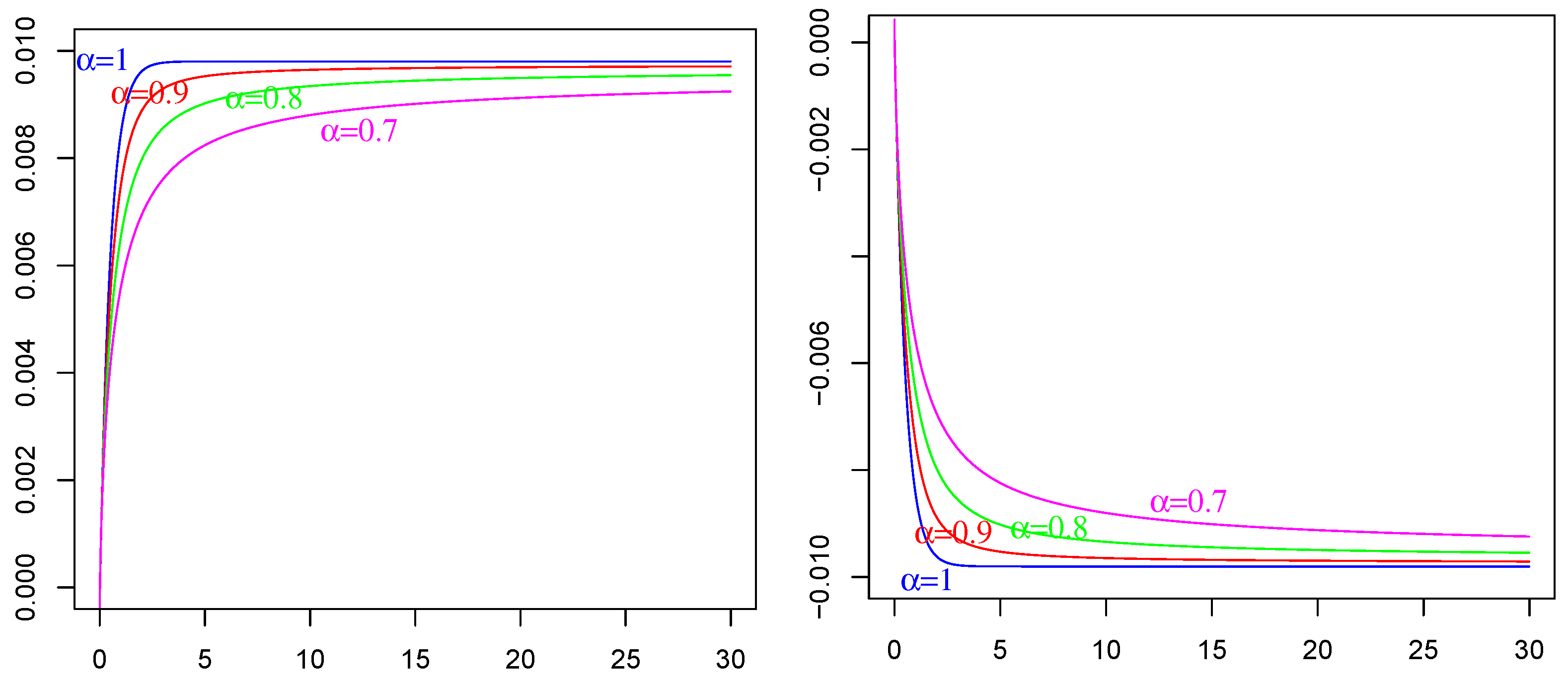
In Figure 2 we plot means, $\mathbb{E}\left[\eta \right(t\left)\right]$ as given in (52) for two different choices of the current term I, as specified in the caption. These means can also be viewed as specific cases of $\mathbb{E}\left[X\right(t\left)\right]$ given in (18). In this figure, different plots correspond to different values of the fractional $\alpha$. It is possible to see in both cases (on left and right) of applied currents I that the decay towards the asymptotic value I is faster when $\alpha =1$, and it becomes slower and slower as values of $\alpha$ decrease. This sort of slowdown is typical of fractional dynamics with respect to those (classical) of an integer order.

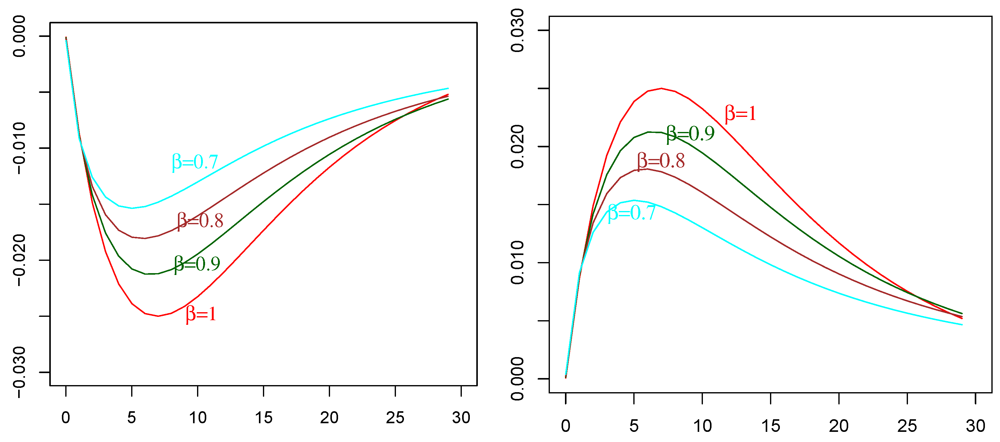
In Figure 3, we plot the means $\mathbb{E}\left[V\right(t\left)\right]$ as in (56) for different $\beta$ values. These means can also be viewed as particular cases of $\mathbb{E}\left[Y\right(t\left)\right]$ given in (33). In this figure, the plots correspond to different values of the fractional $\beta$, whereas $\alpha =1$ for the corresponding input process $\eta \left(t\right)$. The resting potential value $V_L$ and the input current term I are chosen as $V_L=-0.1,I=0.01$ on the left and $V_L=0.1,I=-0.01$ on the right. On the left: the initial attraction towards negative values is evident due to the presence of the resting potential value $V_L<0$, and then due to the successive increasing behavior of the applied positive current $I.$ The overall behaviors regarding different values of $\beta$ appear ordered as $\beta$ varies. In particular, for $\beta =1$, the mean behavior of $V\left(t\right)$ appears more sensitive to the presence of $V_L$ because it assumes the lowest values with respect to other cases. Moreover, it seems to attain the equilibrium level more rapidly ( see the tail of plots for large time values greater than 25). On the right: the same considerations can be made even if the plots are symmetrically (with the opposite sign) identical to those on the left due to the opposite (in sign) choices of parameters $V_L$ and $I.$

In Figure 4, we plot $\mathbb{E}\left[V\right(t\left)\right]$ as in (56) for different values of $\alpha$ and $\beta$. These plots are particular cases of $\mathbb{E}\left[Y\right(t\left)\right]$ given in (33). Looking at the plots from the left to the right, i.e., for increasing values of $\beta ,$ the mean varies on a wider range of values, which means that the mean of the potential is affected more by the joint action of the presence of the resting potential and of the input process. Such a feature holds for all considered values of $\alpha .$ Looking inside each sub-figure, the slowdown in the evolution is evident and ordered as the values of $\alpha$ decrease.

A final consideration can be made: the numerical and graphical analyses of the mean functions $\mathbb{E}\left[\eta \right(t\left)\right]$, $\mathbb{E}\left[V\right(t\left)\right]$, of the input process and voltage process, respectively, reveal that a wider range than that of the classical case of possible evolutions concerning neuronal dynamics can be described by the proposed model (50). This also means that for suitable choices of fractional orders, the model can fit neuronal data that are not described well by classical models. In particular, the evolution time scale of the input and of the voltage can be tuned appropriately in accordance with the neuro-physiological data requirements.

5.2. About the Covariance Functions

For the covariance functions $Cov\left[\eta \right(u),\eta (t\left)\right]$ and $Cov\left(V\right(u),V(t\left)\right)$, we show and discuss the plots obtained from numerical evaluations of Equations (53) and (58), respectively. These plots coincide with those of $Cov\left[X\right(u),X(t\left)\right]$ as in (20) and $Cov\left(Y\right(u),Y(t\left)\right)$ as in (42), respectively, for specified settings of involved parameters and functions. We also consider Equation (49) for $Cov\left(Y\right(u),Y(t\left)\right)$ when we set $\alpha =1.$

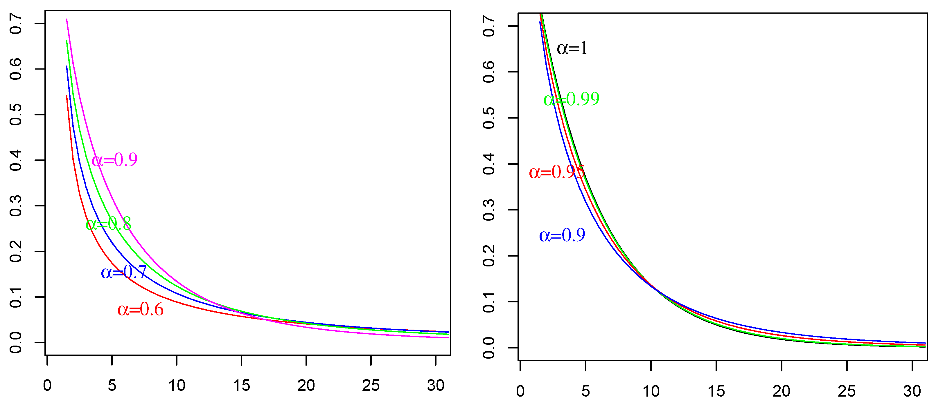
In Figure 5, we plot covariance $Cov\left[\eta \right(u),\eta (t\left)\right]$ given in (53). These plots are particular cases of $Cov\left[X\right(u),X(t\left)\right]$ as in (20). From such graphical representations, we understand that such covariance attains initially higher values in correspondence of higher values of $\alpha$; then, the inverse occurs: on the tails, the decaying of the covariance is slower for smaller values of $\alpha .$ This is related to the long-range property of this type of process. Moreover, it is possible to note the perfect agreement with the integer (classical) case for $\alpha =1$ when the value of $\alpha$ increases from $0.6$ to $0.99.$

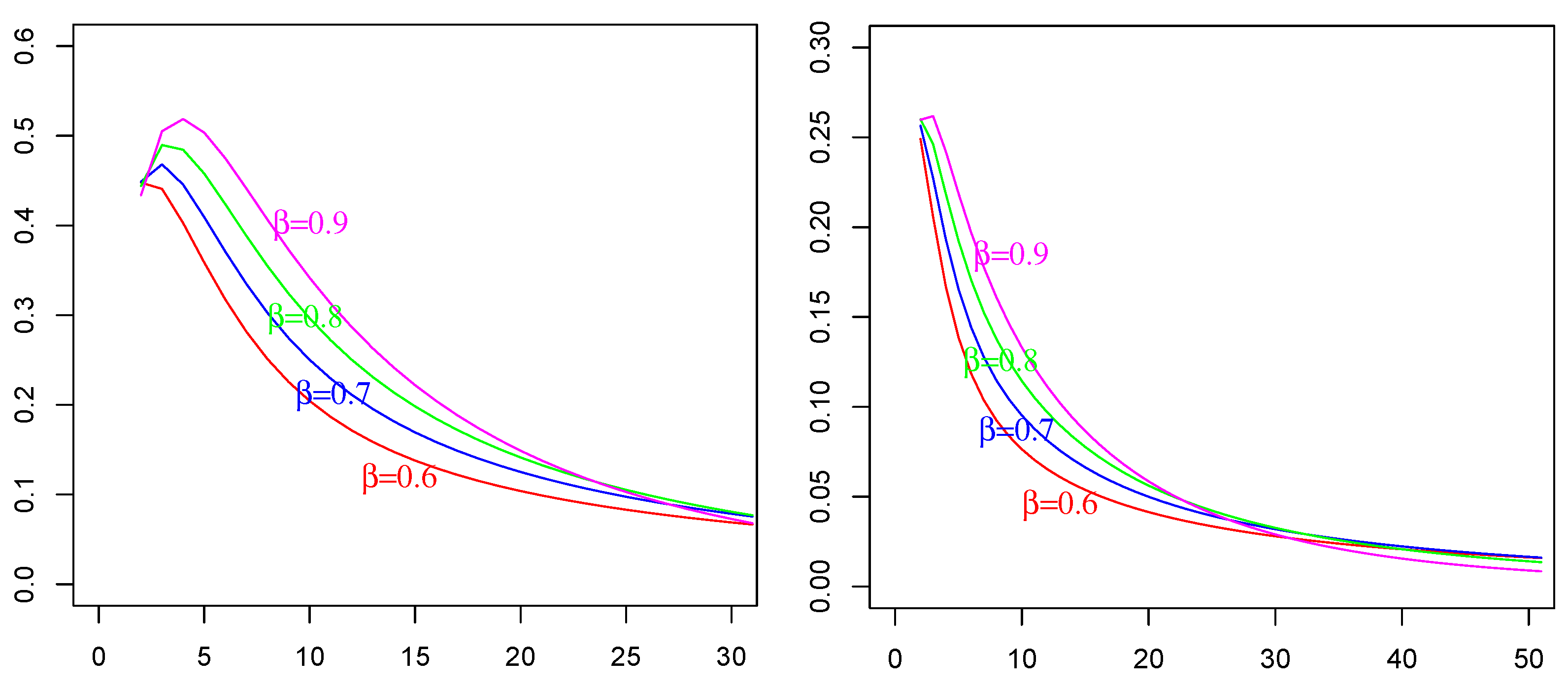
In Figure 6, we provide plots of $Cov\left(V\right(u),V(t\left)\right)$ as in (58) for $u=1$, $t>u$, $\alpha =1$ and for some values of $\beta$. Such plots are the same as for the $Cov\left(Y\right(u),Y(t\left)\right)$ obtained from (49). We note that these numerical evaluations initially show increasing values of the $Cov\left(V\right(u),V(t\left)\right)$ in correspondence of increasing values of $\beta$ (see Figure 6, left), but this behavior changes and inverts for large values of time $t,$ as it is possible to see in the tails of plots on the right of Figure 6. We already observed this similar behavior for $Cov\left[\eta \right(u),\eta (t\left)\right]$ in Figure 5. Hence, $V\left(t\right)$ inherits this type of feature, which is, again, related to the long-range dependence property that such covariance preserves. This will be further investigated from a theoretical point of view and via successive numerical optimized evaluations.

In Figure 7, Figure 8 and Figure 9, we provide plots of $Cov\left(V\right(u),V(t\left)\right)$ as in (58) with varying u and t values, and for three values of $\beta =0.6,0.8,0.99$. Such plots are the same of the $Cov\left(Y\right(u),Y(t\left)\right)$ obtained from (49) for a suitable setting of involved parameters and functions. By comparing plots of Figure 7, Figure 8 and Figure 9, which correspond to the plots for values of $\beta$ in an increasing order, we note that the covariance $Cov\left(V\right(u),V(t\left)\right)$ attains increasing values: from the maximum value $1.4$ in Figure 7 to the maximum value $4.5$ in Figure 9. Moreover, from the observation of color maps on left of Figure 7, Figure 8 and Figure 9, the extension of the region of plane $(u,t),$ corresponds to the highest values of covariance and stretches around the variance diagonal as $\beta$ values increase. This can be also interpreted by saying that the covariance persists over a longer time period for increasing values of $\beta .$ Finally, the value of the covariance increases as u and t both increase.

This in-depth study and the provided plots of the covariances $Cov\left(X\right(u),X(t\left)\right)$ and $Cov\left(Y\right(u),Y(t\left)\right),$ especially after the investigation by means of three-dimensional visualizations, confirm the inclusion of an amount of “memory” in these types of models. The provided representations of such functions allowed for these exploration results to be obtained and for the validation of theoretical properties. They also opened up the possibility to use them in many different further modeling frameworks.

6. Some Concluding Remarks

Motivated by the wish to provide more refined neuronal models, including some memory effects, we studied the solution processes of a couple of fractional stochastic differential equations (Equations (1) and (2)) involving Caputo-fractional derivatives. Such processes are ML fractional processes, as specified in (21) and (30), respectively. In order to provide compact expressions of such processes and of their means and covariances, we introduced the ML fractional integral operators: a deterministic one as in (14) and a stochastic one as in (15) with respect to standard Brownian motion. The main results are in Theorems 1 and 2, in which the representation Formulas (17) and (32) are given for processes X and $Y$, respectively, in terms of the ML fractional operators. Such representations turn out extremely useful for determining computable new expressions of the covariances (20) of X and (35) for Y, but they also allow us to understand the roles and the resulting effects of processes in the coupled dynamics. This is extremely useful when we assign physical values to all involved functions, parameters and processes, as we demonstrated in the provided application to the neuronal model (50) in Section 4 and Section 5.

We remark that the studied processes are Gaussian non-Markovian with a long-range dependence property. The provided results allow us to devise simulation algorithms for these types of processes, such as those based on exact generating procedures of Gaussian random variables: this is now possible due to the explicit computable form of the covariances, which are provided here. (We recall that, in particular, many direct computations of ML fractional integrals, in simple cases, are available in [11,12]).

The Figures show that numerical and quantitative analyses of covariances of such processes are possible, and they has to be carried out in a systematic way. Moreover, we understand that a more rigorous and in-depth study of ML stochastic fractional integrals and processes is also necessary, due the mathematical beauty and the practical interest of such operators. All these proposed research objectives will be developed in our future works.

References

1. Abundo, M.; Pirozzi, E. Fractionally integrated Gauss-Markov processes and applications. Commun. Nonlinear Sci. Numer. Simul. 2021, 101, 105862. [Google Scholar] [CrossRef]
2. Anh, P.T.; Doan, T.S.; Huong, P.T. A variation of constant formula for Caputo fractional stochastic differential equations. Stat. Probab. Lett. 2019, 145, 351–358. [Google Scholar] [CrossRef]
3. Li, K.; Peng, J. Laplace transform and fractional differential equations. Appl. Math. Lett. 2011, 24, 2019–2023. [Google Scholar]
4. Pirozzi, E. Some Fractional Stochastic Models for Neuronal Activity with Different Time-Scales and Correlated Inputs. Fractal Fract. 2024, 8, 57. [Google Scholar] [CrossRef]
5. Teka, W.; Marinov, T.M.; Santamaria, F. Neuronal Spike Timing Adaptation Described with a Fractional Leaky Integrate-and-Fire Model. PLoS Comput. Biol. 2014, 10, e1003526. [Google Scholar] [CrossRef]
6. Luchko, Y. General Fractional Integrals and Derivatives of Arbitrary Order. Symmetry 2021, 13, 755. [Google Scholar] [CrossRef]
7. Kochubei, A.N. General fractional calculus, evolution equations, and renewal processes. Integr. Equ. Oper. Theory 2011, 71, 583–600. [Google Scholar] [CrossRef]
8. Fernandez, A.; Özarslan, M.A.; Baleanu, D. On fractional calculus with general analytic kernels. In Applied Mathematics and Computation; Elsevier: Amsterdam, The Netherlands, 2019; Volume 354, pp. 248–265. [Google Scholar]
9. Giusti, A.; Colombaro, I.; Garra, R.; Garrappa, R.; Polito, F.; Popolizio, M.; Mainardi, F. A Practical Guide to Prabhakar Fractional Calculus. Fract. Calc. Appl. Anal. 2020, 23, 9–54. [Google Scholar] [CrossRef]
10. Polito, F.; Tomovski, Z. Some Properties of Prabhakar-type fractional calculus operators. Fract. Differ. Calc. 2016, 6, 73–94. [Google Scholar] [CrossRef]
11. Haubold, H.J.; Mathai, A.M.; Saxena, R.K. Mittag-Leffler functions and their applications. J. Appl. Math. 2011, 51, 298628. [Google Scholar] [CrossRef]
12. Ascione, G.; Mishura, Y.; Pirozzi, E. Fractional Deterministic and Stochastic Calculus; De Gruyter: Berlin, Germany, 2024. [Google Scholar]
13. Samko, S.G.; Kilbas, A.A.; Marichev, O.I. Fractional Integrals and Derivatives: Theory and Applications; Gordon and Breach Science Publishers: London, UK, 1993. [Google Scholar]
14. Baccouch, M.; Temimi, H.; Ben-Romdhane, M. A discontinuous Galerkin method for systems of stochastic differential equations with applications to population biology, finance, and physics. J. Comput. Appl. Math. 2021, 388, 113297. [Google Scholar] [CrossRef]
15. Batiha, I.M.; Abubaker, A.A.; Jebril, I.H.; Al-Shaikh, S.B.; Matarneh, K. A Numerical Approach of Handling Fractional Stochastic Differential Equations. Axioms 2023, 12, 388. [Google Scholar] [CrossRef]
16. Diethelm, K. The Analysis of Fractional Differential Equations, Lecture Notes in Mathematics 2004; Springer: Berlin/Heidelberg, Germany, 2010. [Google Scholar] [CrossRef]
17. Podlubny, I. Fractional Differential Equations; Academic Press: New York, NY, USA, 1999. [Google Scholar]
18. Garra, R.; Gorenflo, R.; Polito, F.; Tomovski, Z. Hilfer–Prabhakar derivatives and some applications. Appl. Math. Comput. 2014, 242, 576–589. [Google Scholar] [CrossRef]
19. Kilbas, A.A.; Saigo, M.; Saxena, R.K. Generalized mittag-leffler function and generalized fractional calculus operators. Integral Transform. Spec. Funct. 2004, 15, 31–49. [Google Scholar] [CrossRef]
20. Prabhakar, T.R. A singular integral equation with a generalized Mittag Leffler function in the kernel. Yokohama Math. J. 1971, 19, 7–15. [Google Scholar]
21. Garrappa, R.; Kaslik, E.; Popolizio, M. Evaluation of Fractional Integrals and Derivatives of Elementary Functions: Overview and Tutorial. Mathematics 2019, 7, 407. [Google Scholar] [CrossRef]
22. Meerschaert, M.M.; Sabzikar, F. Tempered fractional Brownian motion. Stat. Probab. Lett. 2013, 83, 2269–2275. [Google Scholar] [CrossRef]
23. Ascione, G.; Pirozzi, E. On a stochastic neuronal model integrating correlated inputs. Math. Biosci. Eng. 2019, 16, 5206–5225. [Google Scholar] [CrossRef]
24. Sakai, Y.; Funahashi, S.; Shinomoto, S. Temporally correlated inputs to leaky integrate-and-fire models can reproduce spiking statistics of cortical neurons. Neural Netw. 1999, 12, 1181–1190. [Google Scholar] [CrossRef]
25. Shinomoto, S.; Sakai, Y.; Funahashi, S. The Ornstein-Uhlenbeck process does not reproduce spiking statistics of cortical neurons. Neural Comput. 1997, 11, 935–951. [Google Scholar] [CrossRef]
26. Kim, H.; Shinomoto, S. Estimating nonstationary inputs from a single spike train based on a neuron model with adaptation. Math. Bios. Eng. 2014, 11, 49–62. [Google Scholar] [CrossRef]
27. Leonenko, N.; Meerschaert, M.M.; Schilling, R.L.; Sikorskii, A. Correlation Structure of Time-Changed Lévy Processes. Commun. Appl. Ind. Math. 2014, 6, e-483. [Google Scholar] [CrossRef]
28. Doan, T.S.; Kloeden, P.; Huong, P.; Tuan, H.T. Asymptotic separation between solutions of Caputo fractional stochastic differential equations. Stoch. Anal. Appl. 2018, 36, 654–664. [Google Scholar]
29. Wang, Y.; Xu, J.; Kloeden, P.E. Asymptotic behavior of stochastic lattice systems with a Caputo fractional time derivative. Nonlinear Anal. 2016, 135, 205–222. [Google Scholar] [CrossRef]
30. Bénichou, O.; Oshanin, G. A unifying representation of path integrals for fractional Brownian motions. J. Phys. A Math. Theor. 2024, 57, 225001. [Google Scholar] [CrossRef]
31. Picard, J. Representation formulae for the fractional Brownian motion. In Séminaire de Probabilités XLIII; Springer: Berlin/Heidelberg, Germany, 2011; pp. 3–70. [Google Scholar]
32. Baldi, P. Stochastic Calculus: An Introduction through Theory and Exercises; Universitext; Springer: Berlin/Heidelberg, Germany, 2017. [Google Scholar] [CrossRef]
33. Burkitt, A.N. A review of the integrate-and-fire neuron model: I. Homogeneous synaptic input. Biol. Cybern. 2006, 95, 1–19. [Google Scholar] [CrossRef]
34. Burkitt, A.N. A review of the integrate-and-fire neuron model: II. Inhomogeneous synaptic input and network properties. Biol. Cybern. 2006, 95, 97–112. [Google Scholar] [CrossRef]
35. Tuckwell, H.C. Spatial neuron model with two-parameter Ornstein-Uhlenbeck input current. Phys. A Stat. Mech. Its Appl. 2006, 368, 495–510. [Google Scholar] [CrossRef]
36. Lansky, P. Sources of periodical force in noisy integrate-and-re models of neuronal dynamics. Phys. Rev. E 1997, 55, 2040–2043. [Google Scholar] [CrossRef]
37. Stevens, C.F.; Zador, A.M. Novel integrate-and-fire-like model of repetitive firing in cortical neurons. In Proceedings of the 5th Joint Symposium on Neural Comput, La Jolla, CA, USA, 5 May 1998; Volume 8, pp. 172–177. [Google Scholar]
38. Ascione, G.; Toaldo, B. A Semi-Markov Leaky Integrate-and-Fire model. Mathematics 2019, 7, 1022. [Google Scholar] [CrossRef]
39. Bazzani, A.; Bassi, G.; Turchetti, G. Diffusion and memory effects for stochastic processes and fractional Langevin equations. Phys. A Stat. Mech. Appl. 2003, 324, 530–550. [Google Scholar] [CrossRef]
40. Benedetto, E.; Polito, F.; Sacerdote, L. On firing rate estimation for dependent interspike intervals. Neural Comput. 2015, 27, 699–724. [Google Scholar] [CrossRef] [PubMed]
Figure 1. Comparison between plots of C o v ( Y ( u ) , Y ( t ) ) given by (48) (Blue) and (49) (Red) for u = 1 and t > u . On left: discretization step 0.5 and for t ( 1 , 30 ) ; on right: the zoom for t ( 1 , 7 ) with discretization step 0.1 . Other parameters: β = 0.6 , σ = ς = 1 , a = 0.2 , g = 0.1 .
Mathematics 12 03094 g001
Figure 2. Plots of the mean input E [ η ( t ) ] as given in (52) with I = 0.01 on the left, with I = 0.01 on the right, τ = 5 , η 0 = 0 , for different values of α . These are also the plots of E [ X ( t ) ] given in (18) with X 0 = 0 , A = 1 / τ , B ( t ) I / τ .
Mathematics 12 03094 g002
Figure 3. Plots of mean voltages E [ V ( t ) ] as in (56) with V 0 = 0 , C m = 1 , g L = 0.1 , g = g L C m , for different values of β . About the coupled input process η ( t ) , we set α = 1 , and the same values of the remaining parameters are set as in Figure 2. These plots are also particular cases of E [ Y ( t ) ] given in (33) with y 0 = 0 , h ( t ) g L V L C m , ς = 1 / C m . On the left: V L = 0.1 , I = 0.01 . On the rigth: V L = 0.1 , I = 0.01 .
Mathematics 12 03094 g003
Figure 4. Plots of E [ V ( t ) ] as given in (56) with V L = 0.1 , V 0 = 0 , C m = 1 , g L = 0.1 , g = g L C m , for different values of α and β . Parameters for η ( t ) are τ = 5 , η 0 = 0 , I = 0.01 . These are also plots of E [ Y ( t ) ] given in (33) with y 0 = 0 , h ( t ) g L V L C m , ς = 1 / C m .
Mathematics 12 03094 g004
Figure 5. Plots of covariance C o v [ η ( u ) , η ( t ) ] given in (53) for u = 1 and t > u , with τ = 5 , σ / τ = 1 and for different values of α . These plots are particular cases of C o v [ X ( u ) , X ( t ) ] as in (20) with A = 1 / τ and σ ( t ) σ / τ .
Mathematics 12 03094 g005
Figure 6. Plots of C o v ( V ( u ) , V ( t ) ) as given in (58) for u = 1 and t > u , and for some values of β . On the left: τ = 2 and t ( 1 , 30 ) ; on the right: τ = 1 and t ( 1 , 50 ) (with discretization step 1). Other parameters: σ = 1 , C m = 1 , g L = 0.1 . These are also plots of C o v ( Y ( u ) , Y ( t ) ) obtained from (49), with a = 1 / τ , ς = 1 / C m , g = g L C m .
Mathematics 12 03094 g006
Figure 7. For β = 0.6 and α = 1 : Plots of C o v ( V ( u ) , V ( t ) ) as in (58), or C o v ( Y ( u ) , Y ( t ) ) as in (49), with varying values of u and t. On the left and in the middle: three-dimensional plots from different perspectives; on the right: two-dimensional color map of the same C o v ( V ( u ) , V ( t ) ) . Here, the discretization step is 1, a = 1 / τ = 1 ; other parameters are the same as in Figure 6.
Mathematics 12 03094 g007
Figure 8. For β = 0.8 and α = 1 : Plots of C o v ( V ( u ) , V ( t ) ) as in (58), or C o v ( Y ( u ) , Y ( t ) ) as in (49), with varying values of u and t. On the left and in the middle: three-dimensional plots from different perspectives; on the right: two-dimensional color map of the same C o v ( V ( u ) , V ( t ) ) . Here, the discretization step is 1, a = 1 / τ = 1 ; other parameters are the same as in Figure 6.
Mathematics 12 03094 g008
Figure 9. For β = 0.99 and α = 1 : Plots of C o v ( V ( u ) , V ( t ) ) as in (58), or C o v ( Y ( u ) , Y ( t ) ) as in (49), with varying values of u and t. On the left and in the middle: three-dimensional plots from different perspectives; on the right: two-dimensional color map of the same C o v ( V ( u ) , V ( t ) ) . Here, the discretization step is 1, a = 1 / τ = 1 ; other parameters are the same as in Figure 6.
Mathematics 12 03094 g009
Disclaimer/Publisher’s Note: The statements, opinions and data contained in all publications are solely those of the individual author(s) and contributor(s) and not of MDPI and/or the editor(s). MDPI and/or the editor(s) disclaim responsibility for any injury to people or property resulting from any ideas, methods, instructions or products referred to in the content.