Inverse Probability-Weighted Estimation for Dynamic Structural Equation Model with Missing Data

Abstract

In various applications, observed variables are missing some information that was intended to be collected. The estimations of both loading and path coefficients could be biased when ignoring the missing data. Inverse probability weighting (IPW) is one of the well-known methods helping to reduce bias in regressions, while belonging to a promising but new category in structural equation models. The paper proposes both parametric and nonparametric IPW estimation methods for dynamic structural equation models, in which both loading and path coefficients are developed into functions of a random variable and of the quantile level. To improve the computational efficiency, modified parametric IPW and modified nonparametric IPW are developed through reducing inverse probability computations but making fuller use of completely observed information. All the above IPW estimation methods are compared to existing complete case analysis through simulation investigations. Finally, the paper illustrates the proposed model and estimation methods by an empirical study on digital new-quality productivity.

1. Introduction

Inverse probability weighting (IPW) is a well-known technique in dealing with missing data problems [1]. On the basis of complete case analysis, IPW rebalances the set of complete cases so as to make it representative of the population and reduce the potential existence of bias. Until now, IPW has been considered and wildly applied in various regression-type applications. However, combining the structural equation model (SEM) with IPW to handle missing data problems is not a well-developed topic.

Different from the classical regression models, the structural equation model investigates the relations among different groups of variables and simultaneously measures the relations within each group. The structural equation model labels “groups” as latent variables (denoted as $\mathcal{LV}$), representing those abstract concepts which cannot be observed directly. Correspondingly, within different groups, the variables are labeled as observed variables, which can be directly observed and can specifically explain the meaning of each group. Mathematically, the relations among the different groups or latent variables can be written through structural model (1), while the relations among each latent variable and its corresponding observed variables can be written through measurement model (2) and (3). All these three equations jointly consitute the structural equation model, which has been investigated by many experts [2,3,4,5,6,7,8,9]. Much of the following research developed the classical structural equation models into quantile-type and even more complex varying-coefficient models [10,11,12,13,14,15].

$${\mathcal{LV}}_{\eta }={\mathcal{P}}_{\gamma }{\mathcal{LV}}_{\xi }+{\mathcal{E}}_{\delta }$$

(1)

$$\mathcal{X}={\mathcal{L}}_X{\mathcal{LV}}_{\xi }+{\mathcal{E}}_X$$

(2)

$$\mathcal{Y}={\mathcal{L}}_Y{\mathcal{LV}}_{\eta }+{\mathcal{E}}_Y$$

(3)

Here, ${\mathcal{LV}}_{\eta }$ and ${\mathcal{LV}}_{\xi }$ represent a vector of the endogenous latent variables and a vector of the exogenous latent variables, respectively. ${\mathcal{P}}_{\gamma }$ represents the path coefficients vector, while ${\mathcal{L}}_X$ and ${\mathcal{L}}_Y$ represent the loading coefficients. The random error term ${\mathcal{E}}_{\delta }$ is assumed to have a mean of 0 and fixed variance for the corresponding latent variable. $\mathcal{X}$ and $\mathcal{Y}$ are vectors of the observed variables for latent variable vectors ${\mathcal{LV}}_{\xi }$ and ${\mathcal{LV}}_{\eta }$, respectively. The random error terms ${\mathcal{E}}_X$ and ${\mathcal{E}}_Y$ are assumed to have a mean of 0 and to be uncorrelated with their corresponding latent variables.

Missing data problems may happen in both latent variables and observed variables. More specifically, latent variables belong to the variables which cannot be directly observed, and thus their values are urgently dependent on the observed variables. However, observed variables sometimes cannot be completely observed due to various reasons. The existence of missing data in observed variables brings huge challenges and difficulty in structural equation model estimations [16,17]. Particularly when the loading and path coefficients are developed into varying functions, estimations with missing data become more complex and hard to handle [18,19,20]. In this case, the simplest approach is to apply complete case analysis (CC), which deletes all the samples if only parts of their information is missing. Ignoring the missing data will waste the observed information, as it will undermine the study efficiency and can sometimes introduce substantial bias.

The paper proposes IPW estimation methods parametrically (denoted as IPW) and nonparametrically (denoted as NIPW) in a dynamic structural equation model with missing data. Our dynamic structural equation model is different from Fang and Wang (2024)’s work [17], which is based on vector autoregression (VAR). Our paper focuses on one kind of dynamic structural equation model, which is inspired by quantile varying-coefficient regression. To further improve the efficiencies of information usage and reduce the computation time, both IPW and NIPW are modified to form two new estimation methods. It should be noted that, due to the different features of our dynamic structural equation model, the existing missing data handling methods are not comparable with our IPW and NIPW [16,17,21].

The rest of our paper is organized as follows. We review the existing dynamic structural equation models and estimation methods in Section 2. Then, we present our proposed parametric and nonparametric IPW estimation algorithms and their corresponding modified ones in Section 3. In Section 4, we carry out simulation studies to investigate the performance of our estimation method. We apply our proposed model and estimation method to digital new-quality productivity real data analysis in Section 5, and some final discussions are included in Section 6.

2. Review of Dynamic Structural Equation Models and Estimation Methods

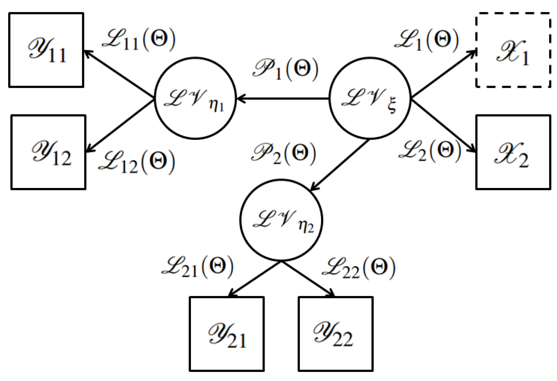
2.1. Dynamic Structural Equation Models with Varying Coefficients

Dynamic structural equation models (DSEMs) mean that the loading and path coefficients are developed into functions of random variables such as time, location, etc. [22,23,24,25,26,27,28,29]. In DSEMs, changing the relations among the latent variables and observed variables can be captured. Assume that time (denoted as $\mathcal{T}$) is the random variable affecting both the varying loading coefficients (denoted as ${\mathcal{P}}_{\gamma }\left(\mathcal{T}\right)$) and path coefficients (denoted as ${\mathcal{L}}_X\left(\mathcal{T}\right)$ and ${\mathcal{L}}_Y\left(\mathcal{T}\right)$). In this situation, the dynamic structural equation model [30] can be written as Equations (4).

$${\mathcal{LV}}_{\eta }={\mathcal{P}}_{\gamma }\left(\mathcal{T}\right){\mathcal{LV}}_{\xi }+{\mathcal{E}}_{\delta }$$

(4)

$$\mathcal{X}={\mathcal{L}}_X\left(\mathcal{T}\right){\mathcal{LV}}_{\xi }+{\mathcal{E}}_X$$

$$\mathcal{Y}={\mathcal{L}}_Y\left(\mathcal{T}\right){\mathcal{LV}}_{\eta }+{\mathcal{E}}_Y$$

Sometimes, investigations on quantile-based structural equation models with varying coefficients are urgently needed [31]. In this situation, varying relations among latent variables and observed variables (denoted as ${\mathcal{P}}_{\gamma }(\mathcal{T},\tau )$, ${\mathcal{L}}_X(\mathcal{T},\tau )$ and ${\mathcal{L}}_Y(\mathcal{T},\tau )$) can be captured at different quantiles $\tau$s according to the following equations [32,33]. It should be noted that the random measurement error terms ${\mathcal{E}}_{\delta }\left(\tau \right)$, ${\mathcal{E}}_X\left(\tau \right)$, and ${\mathcal{E}}_Y\left(\tau \right)$ meet the assumptions that their $\tau$th quantiles equal zero under random variables $\mathcal{T}$ and their corresponding predicting latent variables in Equations (5).

$${\mathcal{LV}}_{\eta }={\mathcal{P}}_{\gamma }(\mathcal{T},\tau ){\mathcal{LV}}_{\xi }+{\mathcal{E}}_{\delta }\left(\tau \right)$$

(5)

$$\mathcal{X}={\mathcal{L}}_X(\mathcal{T},\tau ){\mathcal{LV}}_{\xi }+{\mathcal{E}}_X\left(\tau \right)$$

$$\mathcal{Y}={\mathcal{L}}_Y(\mathcal{T},\tau ){\mathcal{LV}}_{\eta }+{\mathcal{E}}_Y\left(\tau \right)$$

2.2. The Local Polynomial PLS Estimation for Dynamic Structural Equation Models

Partial least square (PLS) and its successors are well-known estimation algorithms used in the background of structural equation models. Especially in dynamic structural equation models, general partial least square cannot accomplish the estimation of both loading and path coefficients. In this situation, the local polynomial method under the framework of PLS is welcomed to solve the dynamic structural equation model problem [30,31].

Local polynomial PLS starts from latent variables’ outer estimation. More specifically, the latent variables can be obtained by calculating the product of their corresponding groups of observed variables with outer weights. The objective function for the estimation of outer weights and the updated procedure can be written as follows:

$$\sum _{i=1}^N{\Phi }_i[{\tilde{\mathcal{Y}}}_{j,i}-\sum _{k=1}^K{\tilde{\mathcal{W}}}_{jk}(\Theta ){\mathcal{Y}}_{jk,i}]$$

(6)

Here, ${\tilde{\mathcal{Y}}}_{j,i}$ is the scaled external estimation of the jth latent variable for the ith sample size, ${\tilde{\mathcal{W}}}_{jk}(\Theta )$ represents the kth estimated parameter of the jth latent variable, and ${\mathcal{Y}}_{jk,i}$ represents the kth observed variable for the jth latent variable of the ith sample size. $\Theta$ represents nothing for classical structural equation models (1)–(3), $\mathcal{T}$ for the dynamic structural equation model (4), and $(\mathcal{T},\tau )$ for the quantile-type dynamic structural equation model (5). According to Taylor’s expansion, ${\tilde{\mathcal{W}}}_{jk}(\Theta )$ in the latter two types of dynamic structural equation models can be written as the following Equation (7) if it is differentiable:

$$\begin{array}{cc}\hfill {\tilde{\mathcal{W}}}_{jk}(\Theta )& \approx {\tilde{\mathcal{W}}}_{jk}(\Theta )+{\tilde{\mathcal{W}}}_{jk}^{\prime }(\Theta )(\mathcal{T}-{\mathcal{T}}_0)+\cdots +{\tilde{\mathcal{W}}}_{jk}^{\left(q\right)}(\Theta ){(\mathcal{T}-{\mathcal{T}}_0)}^q/q!\hfill \\ & =\sum _{l=0}^q{\tilde{\mathcal{W}}}_{jk}^{\left(l\right)}(\Theta ){(\mathcal{T}-{\mathcal{T}}_0)}^l/l!\hfill \end{array}$$

(7)

Taking $q=1$, ${\tilde{\mathcal{W}}}_{jk}(\Theta )$ is estimated through solving the minimization problem [34,35].

$$min\sum _i^N{\Phi }_i\{{\tilde{\mathcal{Y}}}_{j,i}-\sum _{k=1}^K[{\tilde{\mathcal{W}}}_{jk}(\Theta )+{\tilde{\mathcal{W}}}_{jk}^{\prime }(\Theta )(\mathcal{T}-{\mathcal{T}}_0)]{\mathcal{Y}}_{jk,i}\}K[(\mathcal{T}-{\mathcal{T}}_0)/h]$$

Latent variables’ internal estimations can be obtained through the corresponding external estimations multiplied by inner weights [36]. The weight estimation procedure will not stop until it reaches 200 iterations or until the change in the outer weights between two consecutive iterations is smaller than ${10}^{-5}$ at the same time [37].

Using the scaled internal estimation of endogenous latent variables ${\tilde{\mathcal{Z}}}_{en}$ and the scaled internal estimation of exogenous latent variables ${\tilde{\mathcal{Z}}}_{ex}$, path coefficients $\widehat{\tilde{\mathcal{P}}}(\Theta )$ can be estimated according to the following equation:

$$min\sum _i^N{\Phi }_i\{{\tilde{\mathcal{Z}}}_{en,i}-[\tilde{\mathcal{P}}(\Theta )+{\tilde{\mathcal{P}}}^{\prime }(\Theta )(\mathcal{T}-{\mathcal{T}}_0)]{\tilde{\mathcal{Z}}}_{ex,i}\}K[(\mathcal{T}-{\mathcal{T}}_0)/h]$$

The kernel function $K[(\mathcal{T}-{\mathcal{T}}_0)/h]$ is the following Gaussian kernel function. Here, $\delta$ represents the sample standard deviation of the corresponding observed variable vectors or latent variable vectors.

$$K[(\mathcal{T}-{\mathcal{T}}_0)/h]={\displaystyle \frac{1}{{\left(2\pi \right)}^{1/2}}}\ast e^{-{({\displaystyle \frac{\mathcal{T}-{\mathcal{T}}_0}{h}})}^2/2}$$

$$h=\delta \ast N^{-1/3}$$

3. The Proposed IPW Estimation Algorithms

3.1. The Proposed Parametric IPW Estimation Algorithms

In the paper, the dynamic structural equation model estimation investigation is carried out on the basis of the partial least square framework. Let ${\delta }_i$ be the indicator representing whether observed variable ${\mathcal{X}}_1$ is missing. In other words, ${\mathcal{X}}_1$ equals 1 when observable; otherwise, it equals 0. In the situation, inverse probability weighting (IPW) is used to rebalance the set of complete cases, making it representative of the whole sample.

As a weight adjustment (WA), IPW weights all completely observed data by the following equation, which means that the reciprocals of the probabilities are missing ${\mathcal{X}}_{S,i}$ if involved, given the completely observed ${\mathcal{X}}_{S,i}$, ${\mathcal{Y}}_{S,i}$, and ${\mathcal{LV}}_{S,i}$.

$$W{A}_{IPW}={\displaystyle \frac{1}{\Pi ({\mathcal{X}}_{S,i},{\mathcal{Y}}_{S,i},{\mathcal{LV}}_{S,i},{\delta }_i)}}={\displaystyle \frac{1}{\mathrm{prob}({\delta }_i=1|{\mathcal{X}}_{S,i},{\mathcal{Y}}_{S,i},{\mathcal{LV}}_{S,i})}}$$

Here, ${\mathcal{X}}_{S,i}$, ${\mathcal{Y}}_{S,i}$, and ${\mathcal{LV}}_{S,i}$ use S to represent the “selected” observed variables or latent variables for the ith sample. The paper defines the “selected” variable" as those observed or latent variables within one certain regression relationship. More specifically, the estimator of the outer weights ${\tilde{\mathcal{W}}}_{1k}(\Theta )$ for the latent variable ${\mathcal{LV}}_1$ can be estimated through ${\sum }_i^N{\displaystyle \frac{{\delta }_i}{\Pi ({\mathcal{X}}_{11,i},{\mathcal{X}}_{12,i},{\delta }_i)}}{\Phi }_i[{\tilde{\mathcal{Y}}}_{1,i}-{\tilde{\mathcal{W}}}_{11}(\Theta ){\mathcal{X}}_{11,i}-{\tilde{\mathcal{W}}}_{12}(\Theta ){\mathcal{X}}_{12,i}]$, where the “selected” variables consist of $({\mathcal{LV}}_1,{\mathcal{X}}_{11},{\mathcal{X}}_{12})$. Therefore, the estimator of the outer weights ${\tilde{\mathcal{W}}}_{jk}(\Theta )$ can be estimated using the following equation:

$$argmin\sum _i^N{\displaystyle \frac{{\delta }_i{\Phi }_i\{{\tilde{\mathcal{Y}}}_{j,i}-{\sum }_{k=1}^K[{\tilde{\mathcal{W}}}_{jk}(\Theta )+{\tilde{\mathcal{W}}}_{jk}^{\prime }(\Theta )(\mathcal{T}-{\mathcal{T}}_0)]{\mathcal{Y}}_{jk,i}\}K[(\mathcal{T}-{\mathcal{T}}_0)/h]}{\Pi ({\mathcal{X}}_{S,i},{\mathcal{Y}}_{S,i},{\mathcal{LV}}_{S,i},{\delta }_i)}}$$

Correspondingly, the estimator of path coefficients $\widehat{\tilde{\mathcal{P}}}(\Theta )$ can be estimated using the following equation:

$$argmin\sum _i^N{\displaystyle \frac{{\delta }_i{\Phi }_i\{{\tilde{\mathcal{Z}}}_{en,i}-[\tilde{\mathcal{P}}(\Theta )+{\tilde{\mathcal{P}}}^{\prime }(\Theta )(\mathcal{T}-{\mathcal{T}}_0)]{\tilde{\mathcal{Z}}}_{ex,i}\}K[(\mathcal{T}-{\mathcal{T}}_0)/h]}{\Pi ({\mathcal{LV}}_{S,i},{\delta }_i)}}$$

Based on the above investigations, the proposed IPW estimation algorithm can be summarized in dynamic structural equation models with missing data (denoted as Algorithm 1).

Algorithm 1 The proposed IPW estimation algorithm in the dynamic structural equation model

Step 0: Assume the initial values of outer weights. Step 1: External estimation. Use complete cases of observed variables to calculate estimation of latent variables for the Ith iteration. Step 2: Internal estimation. Choose centroid scheme, calculate internal weights, and use the product of internal weights and the external estimation of latent variables to obtain internal estimations for the Ith iteration. Step 3: Update the external weights.       Step 3-1: Estimate the external weights between latent and observed variables using $argmin{\sum }_i^N{\displaystyle \frac{{\delta }_i}{\Pi ({\mathcal{X}}_{S,i},{\mathcal{Y}}_{S,i},{\mathcal{LV}}_{S,i},{\delta }_i)}}{\Phi }_i\{{\tilde{\mathcal{Y}}}_{j,i}-{\sum }_{k=1}^K[{\tilde{\mathcal{W}}}_{jk}(\Theta )+{\tilde{\mathcal{W}}}_{jk}^{\prime }(\Theta )(\mathcal{T}-{\mathcal{T}}_0)]{\mathcal{Y}}_{jk,i}\}K[(\mathcal{T}-{\mathcal{T}}_0)/h]$.       Step 3-2: Calculate the differences of estimated external weights between two consecutive iterations Ith and $(I+1)$th. Step 4: Iterate repeatedly from Step 1 to Step 3.       Step 4-1: Iterate repeatedly until the results meet the stop criterion.       Step 4-2: Obtain the final estimated external weights. Step 5: Estimate the final varying path coefficients using $argmin{\sum }_i^N{\displaystyle \frac{{\delta }_i}{\Pi ({\mathcal{LV}}_{S,i},{\delta }_i)}}{\Phi }_i\{{\tilde{\mathcal{Z}}}_{en,i}-[\tilde{\mathcal{P}}(\Theta )+{\tilde{\mathcal{P}}}^{\prime }(\Theta )(\mathcal{T}-{\mathcal{T}}_0)]{\tilde{\mathcal{Z}}}_{ex,i}\}K[(\mathcal{T}-{\mathcal{T}}_0)/h]$.

3.2. The Proposed Nonparametric IPW Estimation Algorithms

3.2.1. The Determination of the Nonparametric IPW Equation

Nonparametric inverse probability weighting (NIPW), a more complex weight adjustment (WA) than IPW, is based on the approach of Wang, Wang, Zhao, and Ou (1997), using the following kernel smoother [38]:

$$NIPW={\displaystyle \frac{{\sum }_{i=1}^n{\delta }_i{K}_i[(\mathcal{T}-{\mathcal{T}}_0)/h]}{{\sum }_{i=1}^n{K}_i[(\mathcal{T}-{\mathcal{T}}_0)/h]}}$$

As one of the most popular nonparametric smoothing methods, the kernel smoother [35,38,39] depends on the selection of the kernel function $K_i[\ast ]$, the order of the kernel function $\gamma$, the dimensions of the completely observed parts of the variables d, and the bandwidth smoothing parameter h, which will be investigated at length in the following subsections.

3.2.2. The Choice of Kernel Function

A range of commonly used kernel functions are uniform, quadratic, biweight, Gaussian, and others. Several investigation works already exist which use the first three kernel functions. They have at least one point in common. That is, the researchers should pay attention to the range of $\mathcal{T}-{\mathcal{T}}_0$. For example, the uniform kernel function is $K(\mathcal{T}-{\mathcal{T}}_0)={\displaystyle \frac{1}{2}}\ast I_{[-1,1]}(\mathcal{T}-{\mathcal{T}}_0)$. Another more commonly used kernel function is the Gaussian kernel. Like Chen, Wan, and Zhou (2015), although having no compact support in theory, the Gaussian kernel converges to zero at an exponential rate [35]. For example, the Gaussian kernel $K(\mathcal{T}-{\mathcal{T}}_0)=O\left({10}^{-11}\right)$ has practically zero value for u ≥ 5. In addition, with known order $\gamma$, the choice of kernel function usually has little effect on nonparametric estimation and hence has even less of an effect on the estimation of the coefficients [38]. Therefore, the paper chooses the following commonly used Gaussian kernel without alternative kernels in $NIPW$:

$$K(\mathcal{T}-{\mathcal{T}}_0)={\displaystyle \frac{1}{{\left(2\pi \right)}^{1/2}}}{e}^{-{\displaystyle \frac{{(\mathcal{T}-{\mathcal{T}}_0)}^2}{2}}}, where-\infty <\mathcal{T}-{\mathcal{T}}_0<\infty$$

3.2.3. Determining the Order of Kernel Function $\gamma$

A kernel function $K[\ast ]$ is called the $\gamma$th order kernel function if it satisfies the following properties. For simplicity, the paper sets $u=\mathcal{T}-{\mathcal{T}}_0$, and we consider the kernel function $K[\ast ]$ as a Gaussian kernel.

$$\int K(u)du=1,$$

(8)

$$\int u^{m}K\left(u\right)du=0, form=1,\cdots ,(\gamma -1),$$

(9)

$$\int u^{\gamma }K\left(u\right)du\ne 0,$$

(10)

$$\int K^2\left(u\right)du<\infty$$

(11)

Condition (8) means the sum of the weights equals one. Condition (9) is a type of symmetry condition. For example, $\int uK\left(u\right)du=0$ is equivalent to $K(-u)=K\left(u\right)$. Condition (10) shows the order of the kernel function $K[\ast ]$. Condition (11) indicates that the kernel function $K[\ast ]$ is bounded. More strictly, the above four conditions are necessary for $K[\ast ]$ to be a boundary kernel. In fact, many kernels can be modified to obtain boundary kernels [40].

According to the above investigation, the paper calculates the order of the selected targeting Gaussian kernel (denoted as $\gamma$). Conditions (8) and (9) are obviously satisfied when $m=1$ because it is a kind of probability density function and is symmetric. Here are the detailed proofs of condition (10) when $\gamma =2$ and condition (11).

Proof for condition (10). 

When $\gamma =2$ and $K[\ast ]$ is chosen as the Gaussian kernel,

$$\begin{array}{cc}\hfill \int u^{\gamma }K\left(u\right)du& =\int u^{2}K\left(u\right)du\hfill \\ & =\int u^2(1/{\left(2\pi \right)}^{1/2})\ast e^{-u^2/2}du\hfill \\ & =(1/{\left(2\pi \right)}^{1/2})\ast \int u^2\ast e^{-u^2/2}du.\hfill \end{array}$$

Refer to the integration formula:

$$\int u^{2n}\ast e^{-u^2/a^2}du=2\ast {\pi }^{1/2}\ast {(a/2)}^{2n+1}\ast \left(2n\right)!/n!,$$

Take $n=1$ and $a=2^{1/2}$,

$$\begin{array}{cc}\hfill \int u^{2n}\ast e^{-u^2/a^2}du& =\int u^2\ast e^{-u^2/2}du\hfill \\ & ={\left(2\pi \right)}^{1/2}\hfill \end{array}$$

Therefore,

$$\begin{array}{cc}\hfill \int u^{\gamma }K\left(u\right)du& =(1/{\left(2\pi \right)}^{1/2})\ast {\left(2\pi \right)}^{1/2}\hfill \\ & =1\ne 0.\hfill \end{array}$$

□

Proof for condition (11). 

Because

$$\int K^2\left(u\right)du=\int (1/2\pi )\ast e^{-u^2}du$$

Refer to the integration formula:

$$\int e^{-a\ast u^2}du={(\pi /a)}^{1/2}$$

Easily, the paper obtains the result:

$$\begin{array}{cc}\hfill \int K^2\left(u\right)du& =(1/2\pi )\ast {\left(\pi \right)}^{1/2}\hfill \\ & =1/2{\pi }^{1/2}<\infty \hfill \end{array}$$

Based on the above calculation process, the final order of the kernel function is determined as $\gamma$ equals 2. □

3.2.4. Determining the Dimension of W, d

For brevity, let W denote all the completely observed variables, shuffle the elements of W and divide them into two parts of $W^{observed}$ and $W^{missing}$. Here, $W^{observed}$ is observed for all subjects, while $W^{missing}$ contains elements for which observations are missing for some subjects.

Actually, d denotes the number of the completely observed and continuous parts of W. The paper requires the continuity here, partially because we will calculate the standard deviation of W. Chen, Wan, and Zhou (2015) and Zhou, Wan, and Wang (2008) take 1 for simplicity [35,41]. In this case, W is organized as ${[Y,Z]}_{2q\ast 1}$, where both Y and Z are univariate. For example, if $Y={(1,2,3)}^T$ and $Z={(4,5,6)}^T$, then $W={(1,2,3,4,5,6)}^T$. Chen, Wan, and Zhou (2015) calculate the bandwidth $h=std[x2;x3;y]/n^{1/3}$ by matlab [35]. Here, $x2$, $x3$, and y represent all completely observed variables and $x1$ represents the only covariate with missing data. Thus, $[x2;x3;y]$ is a $3n\ast 1$ vector, where n is the sample size of $x2$ (same as $x3$ and y). Therefore, the final dimension of W is chosen as $d=1$.

3.2.5. Selecting Bandwidth Smoothing Parameter h

In order to ensure that $n^{1/2}(\widehat{\beta }-\beta )$ is an asymptotic normal distribution with a mean of 0 and an estimated covariance matrix like $1/n\ast M^{-1}\Gamma M^{-1}$, the bandwidth h should satisfy at least two conditions:

$$\left(1\right)n{h}^{2d}\to \infty ,d>0,$$

$$\left(2\right)n{h}^{2\gamma }\to 0,\gamma >0$$

There are several bandwidth selection methods such as the ad hoc method and plug-in method. (Also, there are some criteria such as generalized cross-validation (GCV), unbiased risk (UBR), and the approximate asymptotic mean integrated squared error (MISE) for practical use.) However, a plug-in bandwidth selection seems very complex for practical use because of higher-order covariance calculations [42]. Here, we use a simple ad hoc bandwidth selection method, which does have the correct rate of convergence and is easily programmed and thus h can be written as $h=C\ast n^L$, where C is a constant depending on the unknown function $E\{\Psi (Y,Z,{\beta }_0)|X\}$ and its first and second derivatives. Carroll and Wand (1991) estimated C by calculating the sample standard deviation of the always observed vector of variables W (denoted as ${\delta }_W$) in their papers [43]. $n^L$ indicates the bandwidth rate. We can easily obtain $L>-1/2d$ and $L<-1/2\gamma$ because of the above two conditions, where $n{h}^{2d}\to \infty$ and $n{h}^{2\gamma }\to 0$. Thus, we obtain $d<\gamma$. Carroll and Wand (1991) took $n^L=n^{-1/3}$ directly as the optimal bandwidth rate [43]. Furthermore, Chen, Wan, and Zhou (2015) provide the optimal bandwidth as $O\left(n^{-1/(d+\gamma )}\right)$ and indicate that $\gamma$ commonly equals 2 [35]. When $\gamma =2$, $d=1$ as $0<d<\gamma$. In this way, L also equals $-1/3$. Thus, the paper takes $h={\delta }_W\ast n^{-1/3}$ as the final bandwidth.

Remark 1. 

A second consideration about bandwidth h is based on Gaussian approximation or Silverman’s (1986) rule of thumb (that is, the bandwidth that minimises the mean integrated squared error, $h=1.06\ast {\delta }_W\ast n^{-1/5}$), although it can yield widely inaccurate estimates when the density is not close to being normal [44]. As the common order γ of kernel function is 2, that is, $n{h}^4\to 0$, then the bandwidth rate $n^{-1/5}$ is not allowed. Therefore, $h=1.06\ast {\delta }_W\ast n^{-1/3}$ may be the second appropriate bandwidth.

3.2.6. NIPW Estimation Algorithms

As a more complex weight adjustment (WA) than IPW, NIPW weights all completely observed data through the following equation:

$$W{A}_{NIPW}={\displaystyle \frac{1}{{\Pi }_N({\mathcal{X}}_{S,i},{\mathcal{Y}}_{S,i},{\mathcal{LV}}_{S,i},{\delta }_i)}}={\displaystyle \frac{{\sum }_{i=1}^n{K}_i[(\mathcal{T}-{\mathcal{T}}_0)/h]}{{\sum }_{i=1}^n{\delta }_i{K}_i[(\mathcal{T}-{\mathcal{T}}_0)/h]}}$$

Here, ${\mathcal{X}}_{S,i}$, ${\mathcal{Y}}_{S,i}$, and ${\mathcal{LV}}_{S,i}$ use S to represent the “selected” observed variables or latent variables for the ith sample which are the same as IPW. Correspondingly, the estimator of outer weights ${\tilde{\mathcal{W}}}_{jk}(\Theta )$ can be estimated referring to the following equation, which can be used in Step 3-1 of Algorithm 1 instead.

$$argmin\sum _i^N{\delta }_i{\displaystyle \frac{{\sum }_{i=1}^n{K}_i[(\mathcal{T}-{\mathcal{T}}_0)/h]}{{\sum }_{i=1}^n{\delta }_i{K}_i[(\mathcal{T}-{\mathcal{T}}_0)/h]}}{\Phi }_i\{{\tilde{\mathcal{Y}}}_{j,i}-\sum _{k=1}^K[{\tilde{\mathcal{W}}}_{jk}(\Theta )+{\tilde{\mathcal{W}}}_{jk}^{\prime }(\Theta )(\mathcal{T}-{\mathcal{T}}_0)]{\mathcal{Y}}_{jk,i}\}K[(\mathcal{T}-{\mathcal{T}}_0)/h]$$

The estimator of path coefficients $\widehat{\tilde{\mathcal{P}}}(\Theta )$ can be estimated using the following equation, which can be used in Step 5 of Algorithm 1 instead.

$$argmin\sum _i^N{\delta }_i{\displaystyle \frac{{\sum }_{i=1}^n{K}_i[(\mathcal{T}-{\mathcal{T}}_0)/h]}{{\sum }_{i=1}^n{\delta }_i{K}_i[(\mathcal{T}-{\mathcal{T}}_0)/h]}}{\Phi }_i\{{\tilde{\mathcal{Z}}}_{en,i}-[\tilde{\mathcal{P}}(\Theta )+{\tilde{\mathcal{P}}}^{\prime }(\Theta )(\mathcal{T}-{\mathcal{T}}_0)]{\tilde{\mathcal{Z}}}_{ex,i}\}K[(\mathcal{T}-{\mathcal{T}}_0)/h]$$

3.3. Modified IPW and NIPW Estimation Algorithms

Both IPW and NIPW estimation algorithms are carried out only based on the complete observed cases of all observed variables and latent variables. Under the partial least square algorithm framework, the ’partial’ in IPW and NIPW is reflected in the relatively independent estimations among each latent variable and its corresponding observed variables and among each latent variable. The iteration process for outer weighting updating links all these relatively independent estimations.

For those independent estimations without any variable containing missing data (denoted as ${\mathcal{E}}_1$), a local polynomial PLS estimation algorithm can be directly applied based on all of the variables’ full information. For those independent estimations containing missing data (denoted as ${\mathcal{E}}_2$), IPW or NIPW can be used to correct the biases only using completely observed cases. Although more cases are used to estimate the unknown coefficients which brings a potential computational burden, more observed information is used, and the ellipsis of $W{A}_{IPW}$ and $W{A}_{NIPW}$ calculations is really helpful in improving the computational efficiency. Therefore, modified IPW and NIPW estimation algorithms are proposed.

4. Simulation Investigations

4.1. Notations

Let ${\mathcal{LV}}_{{\eta }_1}$ and ${\mathcal{LV}}_{{\eta }_2}$ represent two endogenous latent variables, and let ${\mathcal{LV}}_{\xi }$ represent exogenous latent variable. For each latent variable, two observed variables are generated, which are denoted as ${\mathcal{Y}}_{11}$, ${\mathcal{Y}}_{12}$, ${\mathcal{Y}}_{21}$, ${\mathcal{Y}}_{22}$, ${\mathcal{X}}_1$, and ${\mathcal{X}}_2$, respectively. We assume that ${\mathcal{X}}_1$ cannot be completely observed, while all of the other observed variables can be completely observed. The loading coefficients ${\mathcal{L}}_{11}(\Theta )$, ${\mathcal{L}}_{12}(\Theta )$, ${\mathcal{L}}_{21}(\Theta )$, ${\mathcal{L}}_{22}(\Theta )$, ${\mathcal{L}}_1(\Theta )$, and ${\mathcal{L}}_2(\Theta )$ link the latent variables to their corresponding observed variables. The path coefficients ${\mathcal{P}}_1(\Theta )$ and ${\mathcal{P}}_2(\Theta )$ link the same exogenous latent variable ${\mathcal{LV}}_{\xi }$ to the endogenous latent variables ${\mathcal{LV}}_{{\eta }_1}$ and ${\mathcal{LV}}_{{\eta }_2}$. Except for the above variables and coefficients, ${\mathcal{E}}_{{\delta }_1}\left(\tau \right)$, ${\mathcal{E}}_{{\delta }_2}\left(\tau \right)$, ${\mathcal{E}}_{{ϵ}_{Y_{1i}}}\left(\tau \right)$, ${\mathcal{E}}_{{ϵ}_{Y_{2j}}}\left(\tau \right)$, and ${\mathcal{E}}_{{ϵ}_{X_k}}\left(\tau \right)$ represent random error terms in dynamic structural equation models with missing data. Let $\delta =1$ if ${\mathcal{X}}_1$ is observed; otherwise, $\delta =0$. Here, $\mathcal{T}$ is a random variable and is typically chosen to be evenly spread across grid points on $(0,1)$ that are sufficiently dense. $\tau$ represents the quantile level.

4.2. Models

Simulated examples are carried out to investigate the proposed IPW estimation algorithms’ performance in applications. The dynamic structural equation models with missing data can be written as the following equations [45,46,47,48]:

$${\mathcal{LV}}_{{\eta }_1}={\mathcal{P}}_1(\Theta ){\mathcal{LV}}_{\xi }+{\mathcal{E}}_{{\delta }_1}\left(\tau \right)$$

$${\mathcal{LV}}_{{\eta }_2}={\mathcal{P}}_2(\Theta ){\mathcal{LV}}_{\xi }+{\mathcal{E}}_{{\delta }_2}\left(\tau \right)$$

$${\mathcal{Y}}_{1i}={\mathcal{L}}_{1i}(\Theta ){\mathcal{LV}}_{{\eta }_1}+{\mathcal{E}}_{{ϵ}_{Y_{1i}}}\left(\tau \right),\forall i=1,2$$

$${\mathcal{Y}}_{2j}={\mathcal{L}}_{2j}(\Theta ){\mathcal{LV}}_{{\eta }_2}+{\mathcal{E}}_{{ϵ}_{Y_{2j}}}\left(\tau \right),\forall j=1,2$$

$${\mathcal{X}}_k={\mathcal{L}}_k(\Theta ){\mathcal{LV}}_{\xi }+{\mathcal{E}}_{{ϵ}_{X_k}}\left(\tau \right),\forall k=1,2$$

Here, $\Theta =(\mathcal{T},\tau )$. Figure 1 displays the dynamic structural equation model with missing data, which illustrates the relations among different latent variables and observed variables more clearly.

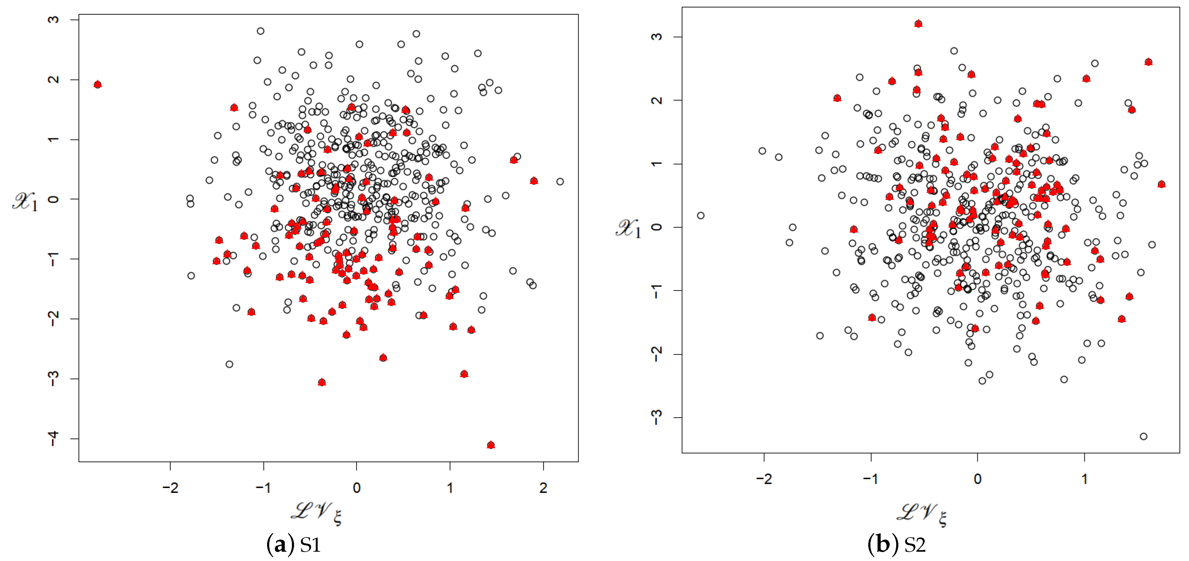
4.3. Simulation Data Generation Mechanism

In the paper, the exogenous latent variable ${\mathcal{LV}}_{\xi }$ is generated from normal distribution $\mathcal{N}(0,(1+\sigma )/(2+\sigma \left)\right)$, where $\sigma$ follows uniform distribution $\mathcal{U}(U/10,2+U/10)$. In the structural model, the random error term ${\mathcal{E}}_{{\delta }_1}\left(\tau \right)$ follows Laplace distribution minus $F^{-1}\left(\tau \right)$, with $F(\ast )$ being the common cumulative distribution function of normal distribution. The random error terms ${\mathcal{E}}_{{\delta }_2}\left(\tau \right)$ equal ${\mathcal{E}}_{{\delta }_1}\left(\tau \right)$ + $\mathcal{N}(0,1)$. In the measurement model, the random error terms are ${\mathcal{E}}_{{ϵ}_{Y_{1i}}}\left(\tau \right)\sim N(n,0,1)$, ${\mathcal{E}}_{{ϵ}_{Y_{2j}}}\left(\tau \right)\sim N(n,0.25,1.{25}^2)$, and ${\mathcal{E}}_{{ϵ}_{X_k}}\left(\tau \right)\sim N(n,0.2,1)$. We assume that as the sample sizes are 200 and 500, the random variable $\mathcal{T}$ has 200 and 500 values, respectively, which are chosen to be evenly spread grid points on (0, 1). For brevity, the paper only displays the estimated results at the quantile levels 0.10, 0.50, and 0.90. The number of Monte Carlo replicates is 200.

The next important part is to generate the loading and path coefficients, which have been developed into functions of $\Theta$. Firstly, path coefficients functions ${\mathcal{P}}_1(\Theta )$ and ${\mathcal{P}}_2(\Theta )$ are given by the following equations:

$${\mathcal{P}}_1\left(\mathcal{T}\right)=15+20sin\left({\displaystyle \frac{\pi }{60}}\mathcal{T}\right)$$

$${\mathcal{P}}_2\left(\mathcal{T}\right)=20+15sin\left({\displaystyle \frac{\pi }{60}}\mathcal{T}\right)$$

Loading coefficient functions ${\mathcal{L}}_{11}(\Theta )$, ${\mathcal{L}}_{12}(\Theta )$, ${\mathcal{L}}_{21}(\Theta )$, ${\mathcal{L}}_{22}(\Theta )$, ${\mathcal{L}}_1(\Theta )$, and ${\mathcal{L}}_2(\Theta )$ are given by the following equations:

$${\mathcal{L}}_{11}\left(\mathcal{T}\right)=2-3cos\left[(\mathcal{T}-25){\displaystyle \frac{\pi }{15}}\right],{\mathcal{L}}_{12}\left(\mathcal{T}\right)=6-0.2\mathcal{T}$$

$${\mathcal{L}}_{21}\left(\mathcal{T}\right)=-4+{\displaystyle \frac{{(20-\mathcal{T})}^3}{2000}},{\mathcal{L}}_{22}\left(\mathcal{T}\right)=1-2cos\left[(\mathcal{T}-25){\displaystyle \frac{\pi }{15}}\right]$$

$${\mathcal{L}}_1\left(\mathcal{T}\right)=-3+{\displaystyle \frac{{(20-\mathcal{T})}^3}{2000}},{\mathcal{L}}_2\left(\mathcal{T}\right)=1.5-2cos\left[(\mathcal{T}-25){\displaystyle \frac{\pi }{15}}\right]$$

The paper considers two kinds of missing mechanisms for observed variable ${\mathcal{X}}_1$, which are denoted as Setting S1 and Setting S2. More specifically, in S1, $\mathcal{P}\left(\delta \right|{\mathcal{X}}_2)=max{[0,({\mathcal{X}}_2+1)/10)}^{1/20}]$, such that approximately 20% of observations miss ${\mathcal{X}}_1$s. While in S2, $\mathcal{P}\left(\delta \right|{\mathcal{X}}_2,\xi )=1/[1+exp(-1.5+0.5{\mathcal{X}}_2+0.6\xi )]$, such that approximately 20% of observations miss ${\mathcal{X}}_1$s, and the missingness is related to another observed variable ${\mathcal{X}}_2$ and even the corresponding latent variable $\xi$. Figure 2 shows two kinds of missing data distributions based on ${\mathcal{LV}}_{\xi }$ and ${\mathcal{X}}_1$ under the two settings S1 and S2 with sample sizes of 500. In S1, there exist 103 missing ${\mathcal{X}}_1$ among 500 points, and the missing rate is 20.600%. In S2, there exist 101 missing ${\mathcal{X}}_1$ among 500 points, and the missing rate is 20.200%.

4.4. Evaluation Indexes

To evaluate the performances of IPW estimation algorithms, indexes measuring the differences between the estimates and true values of loading and path coefficients are needed. In this part, mean absolute errors (MAEs) and mean squared errors (MSEs) are proposed on the basis of all time points ($t=1,\cdots ,\mathcal{T}$) and Monte Carlo replicates ($b=1,\cdots ,\mathcal{B}$). The MAE and MSE equations to calculate all the loading coefficients (denoted as $\mathcal{L}(\Theta )$ for brevity) and path coefficients (denoted as $\mathcal{P}(\Theta )$ for brevity) can be written as follows [49]:

$$MA{E}_{\mathcal{L}(\Theta )}={\displaystyle \frac{1}{\mathcal{B}}}{\displaystyle \frac{1}{\mathcal{T}}}\sum _{b=1}^{\mathcal{B}}\sum _{t=1}^{\mathcal{T}}|\widehat{{\mathcal{L}}_b}(t,\tau )-{\mathcal{L}}_b(t,\tau )|$$

$$MS{E}_{\mathcal{L}(\Theta )}={\displaystyle \frac{1}{\mathcal{B}}}{\displaystyle \frac{1}{\mathcal{T}}}\sum _{b=1}^{\mathcal{B}}\sum _{t=1}^{\mathcal{T}}{(\widehat{{\mathcal{L}}_b}(t,\tau )-{\mathcal{L}}_b(t,\tau ))}^2$$

Here $\widehat{{\mathcal{L}}_b}(t,\tau )$ is the estimated loading coefficients and ${\mathcal{L}}_b(t,\tau )$ is the true loading coefficients at the tth time point ($t=1,\cdots ,\mathcal{T}$) and the bth Monte Carlo replicate ($b=1,\cdots ,B$).

$$MA{E}_{\mathcal{P}(\Theta )}={\displaystyle \frac{1}{\mathcal{B}}}{\displaystyle \frac{1}{\mathcal{T}}}\sum _{b=1}^{\mathcal{B}}\sum _{t=1}^{\mathcal{T}}|\widehat{{\mathcal{P}}_b}(t,\tau )-{\mathcal{P}}_b(t,\tau )|$$

$$MS{E}_{\mathcal{P}(\Theta )}={\displaystyle \frac{1}{\mathcal{B}}}{\displaystyle \frac{1}{\mathcal{T}}}\sum _{b=1}^{\mathcal{B}}\sum _{t=1}^{\mathcal{T}}{(\widehat{{\mathcal{P}}_b}(t,\tau )-{\mathcal{P}}_b(t,\tau ))}^2$$

Here, $\widehat{{\mathcal{P}}_b}(t,\tau )$ is the estimated path coefficients and ${\mathcal{P}}_b(t,\tau )$ is the true path coefficients at the tth time point ($t=1,\cdots ,\mathcal{T}$) and bth Monte Carlo replicate ($b=1,\cdots ,B$).

4.5. Results

4.5.1. Comparisons of Estimation Accuracy and Efficiency in Setting S1

Table 1. Mean absolute errors (MAEs) of the estimated loading and path coefficients with sample sizes of 200 and 200 Monte Carlo replicates in Setting S1.

		${\mathcal{L}}_{11}\left(\mathbf{\Theta }\right)$	${\mathcal{L}}_{12}\left(\mathbf{\Theta }\right)$	${\mathcal{L}}_1\left(\mathbf{\Theta }\right)$	${\mathcal{L}}_2\left(\mathbf{\Theta }\right)$	${\mathcal{L}}_{21}\left(\mathbf{\Theta }\right)$	${\mathcal{L}}_{22}\left(\mathbf{\Theta }\right)$	${\mathcal{P}}_1\left(\mathbf{\Theta }\right)$	${\mathcal{P}}_2\left(\mathbf{\Theta }\right)$
0.10	CC	1.003	0.461	0.418	1.102	0.425	1.017	1.031	1.029
	IPW	1.022	0.494	0.323	0.609	0.453	1.030	1.015	1.017
	IPWM	1.008	0.427	0.317	0.607	0.399	1.027	1.024	1.023
	NIPW	1.003	0.420	0.316	0.562	0.385	1.025	1.024	1.020
	NIPWM	1.008	0.427	0.317	0.561	0.401	1.028	1.028	1.026
0.50	CC	0.966	0.296	0.362	0.998	0.303	1.000	1.032	1.032
	IPW	0.968	0.298	0.354	0.988	0.304	1.008	1.027	1.024
	IPWM	0.975	0.290	0.348	0.984	0.298	1.004	1.030	1.029
	NIPW	0.977	0.295	0.356	0.994	0.297	1.006	1.030	1.030
	NIPWM	0.975	0.292	0.360	0.996	0.299	1.002	1.028	1.029
0.90	CC	1.013	0.471	0.356	0.940	0.418	1.050	1.022	1.024
	IPW	1.030	0.480	0.578	1.462	0.418	1.056	1.025	1.023
	IPWM	1.033	0.455	0.570	1.453	0.404	1.062	1.022	1.021
	NIPW	1.033	0.525	0.589	1.561	0.451	1.062	1.034	1.032
	NIPWM	1.032	0.457	0.575	1.549	0.404	1.062	1.022	1.022

displays the mean absolute errors of the estimated loading and path coefficients with a sample size of 200 from 200 Monte Carlo replicates at quantile levels 0.10, 0.50, and 0.90 in Setting S1.

Table 2. Mean squared errors (MSEs) of the estimated loading and path coefficients with sample sizes of 200 and 200 Monte Carlo replicates in Setting S1.

		${\mathcal{L}}_{11}\left(\mathbf{\Theta }\right)$	${\mathcal{L}}_{12}\left(\mathbf{\Theta }\right)$	${\mathcal{L}}_1\left(\mathbf{\Theta }\right)$	${\mathcal{L}}_2\left(\mathbf{\Theta }\right)$	${\mathcal{L}}_{21}\left(\mathbf{\Theta }\right)$	${\mathcal{L}}_{22}\left(\mathbf{\Theta }\right)$	${\mathcal{P}}_1\left(\mathbf{\Theta }\right)$	${\mathcal{P}}_2\left(\mathbf{\Theta }\right)$
0.10	CC	1.245	0.316	0.259	1.337	0.275	1.221	1.403	1.394
	IPW	1.325	0.370	0.180	0.513	0.315	1.279	1.364	1.362
	IPWM	1.214	0.273	0.173	0.508	0.244	1.217	1.389	1.382
	NIPW	1.190	0.269	0.167	0.442	0.229	1.198	1.386	1.370
	NIPWM	1.214	0.273	0.170	0.440	0.246	1.219	1.396	1.389
0.50	CC	0.971	0.118	0.194	1.088	0.124	1.039	1.408	1.407
	IPW	0.982	0.124	0.190	1.091	0.126	1.061	1.394	1.387
	IPWM	0.983	0.110	0.178	1.081	0.116	1.044	1.403	1.399
	NIPW	0.993	0.117	0.185	1.096	0.119	1.053	1.404	1.401
	NIPWM	0.982	0.111	0.194	1.098	0.117	1.041	1.400	1.400
0.90	CC	1.233	0.332	0.224	1.028	0.263	1.264	1.386	1.387
	IPW	1.281	0.346	0.470	2.378	0.262	1.291	1.390	1.383
	IPWM	1.265	0.312	0.459	2.352	0.244	1.287	1.387	1.381
	NIPW	1.331	0.408	0.479	2.664	0.304	1.339	1.410	1.402
	NIPWM	1.262	0.314	0.456	2.627	0.245	1.286	1.386	1.383

presents the corresponding mean square errors of the estimated loading and path coefficients under the same setting as Table 1.

Table 3. Mean absolute errors (MAEs) of the estimated loading and path coefficients with sample sizes of 500 and 200 Monte Carlo replicates in Setting S1.

		${\mathcal{L}}_{11}\left(\mathbf{\Theta }\right)$	${\mathcal{L}}_{12}\left(\mathbf{\Theta }\right)$	${\mathcal{L}}_1\left(\mathbf{\Theta }\right)$	${\mathcal{L}}_2\left(\mathbf{\Theta }\right)$	${\mathcal{L}}_{21}\left(\mathbf{\Theta }\right)$	${\mathcal{L}}_{22}\left(\mathbf{\Theta }\right)$	${\mathcal{P}}_1\left(\mathbf{\Theta }\right)$	${\mathcal{P}}_2\left(\mathbf{\Theta }\right)$
CC	0.10	0.998	0.523	0.487	1.198	0.460	0.997	1.017	1.016
	0.50	0.998	0.309	0.354	1.028	0.287	0.980	1.018	1.018
	0.90	1.015	0.493	0.328	0.881	0.437	1.012	1.017	1.016
IPW	0.10	1.006	0.555	0.339	0.569	0.489	1.004	1.013	1.012
	0.50	1.001	0.309	0.341	1.016	0.283	0.979	1.015	1.015
	0.90	1.020	0.512	0.691	1.630	0.448	1.016	1.015	1.015
IPWM	0.10	1.002	0.502	0.342	0.567	0.440	0.998	1.016	1.015
	0.50	1.003	0.305	0.337	1.014	0.283	0.981	1.017	1.016
	0.90	1.020	0.496	0.695	1.635	0.432	1.013	1.014	1.013
NIPW	0.10	0.998	0.456	0.334	0.518	0.405	1.001	1.013	1.011
	0.50	1.002	0.306	0.350	1.023	0.284	0.982	1.016	1.016
	0.90	1.026	0.566	0.705	1.729	0.488	1.020	1.019	1.019
NIPWM	0.10	1.003	0.502	0.336	0.516	0.440	0.998	1.017	1.015
	0.50	1.002	0.304	0.347	1.021	0.283	0.982	1.017	1.017
	0.90	1.019	0.495	0.707	1.735	0.432	1.013	1.015	1.014

and

Table 4. Mean squared errors (MSE) of the estimated loading and path coefficients with sample sizes of 500 and 200 Monte Carlo replicates in Setting S1.

		${\mathcal{L}}_{11}\left(\mathbf{\Theta }\right)$	${\mathcal{L}}_{12}\left(\mathbf{\Theta }\right)$	${\mathcal{L}}_1\left(\mathbf{\Theta }\right)$	${\mathcal{L}}_2\left(\mathbf{\Theta }\right)$	${\mathcal{L}}_{21}\left(\mathbf{\Theta }\right)$	${\mathcal{L}}_{22}\left(\mathbf{\Theta }\right)$	${\mathcal{P}}_1\left(\mathbf{\Theta }\right)$	${\mathcal{P}}_2\left(\mathbf{\Theta }\right)$
CC	0.10	1.311	0.382	0.355	1.555	0.302	1.229	1.355	1.353
	0.50	1.033	0.127	0.183	1.116	0.104	0.987	1.357	1.357
	0.90	1.306	0.347	0.178	0.892	0.286	1.227	1.355	1.353
IPW	0.10	1.364	0.429	0.206	0.445	0.338	1.275	1.347	1.341
	0.50	1.044	0.128	0.170	1.103	0.105	0.989	1.350	1.351
	0.90	1.341	0.366	0.653	2.923	0.295	1.252	1.349	1.347
IPWM	0.10	1.286	0.352	0.209	0.444	0.276	1.200	1.353	1.351
	0.50	1.040	0.122	0.167	1.098	0.100	0.988	1.354	1.353
	0.90	1.320	0.344	0.658	2.939	0.275	1.227	1.348	1.344
NIPW	0.10	1.237	0.299	0.198	0.377	0.240	1.178	1.345	1.340
	0.50	1.042	0.125	0.175	1.116	0.103	0.992	1.354	1.352
	0.90	1.415	0.439	0.657	3.238	0.345	1.309	1.359	1.358
NIPWM	0.10	1.287	0.351	0.201	0.374	0.276	1.200	1.355	1.352
	0.50	1.040	0.122	0.173	1.110	0.100	0.988	1.355	1.354
	0.90	1.318	0.344	0.659	3.254	0.275	1.227	1.351	1.348

display the mean absolute errors and mean square errors of the estimated loading and path coefficients with an increased sample size of 500. Obviously, larger mean absolute errors and mean square errors mean relatively worse estimation accuracy. Compared with CC at quantile levels 0.1 and 0.50, our proposed IPW, IPWM, NIPW, and NIPWM estimation algorithms have advantages in all path coefficients estimations, as well as the advantage of the block of loading coefficients (${\mathcal{L}}_1(\Theta )$ and ${\mathcal{L}}_2(\Theta )$) estimation containing missing observed variables. It indicates that in Setting S1, our proposed estimation algorithms are more appropriate for use to capture structural relations among different latent variables and measure the relations between the latent variables and observed variables with missing data at low and median quantile levels. However, at a high quantile level of 0.9 or for those loading coefficients without missing data, the proposed IPW, IPWM, NIPW, and NIPWM estimation algorithms have not showed any substantial advantages.

4.5.2. Comparisons of Estimation Accuracy and Efficiency in Setting S2

Table 5. Mean absolute errors (MAEs) of the estimated loading and path coefficients with sample sizes of 200 and 200 Monte Carlo replicates in Setting S2.

		${\mathcal{L}}_{11}\left(\mathbf{\Theta }\right)$	${\mathcal{L}}_{12}\left(\mathbf{\Theta }\right)$	${\mathcal{L}}_1\left(\mathbf{\Theta }\right)$	${\mathcal{L}}_2\left(\mathbf{\Theta }\right)$	${\mathcal{L}}_{21}\left(\mathbf{\Theta }\right)$	${\mathcal{L}}_{22}\left(\mathbf{\Theta }\right)$	${\mathcal{P}}_1\left(\mathbf{\Theta }\right)$	${\mathcal{P}}_2\left(\mathbf{\Theta }\right)$
0.10	CC	0.975	0.439	0.386	0.999	0.408	1.001	1.018	1.019
	IPW	0.999	0.464	0.574	1.280	0.429	1.023	1.022	1.021
	IPWM	1.013	0.422	0.577	1.284	0.396	1.025	1.018	1.016
	NIPW	1.003	0.472	0.614	1.349	0.438	1.027	1.019	1.016
	NIPWM	1.014	0.422	0.607	1.348	0.395	1.026	1.019	1.019
0.50	CC	0.963	0.298	0.372	0.998	0.300	0.989	1.025	1.024
	IPW	0.972	0.300	0.358	0.981	0.298	0.997	1.023	1.022
	IPWM	0.971	0.289	0.356	0.982	0.297	1.000	1.024	1.023
	NIPW	0.967	0.298	0.370	0.998	0.299	0.994	1.025	1.024
	NIPWM	0.970	0.288	0.368	0.999	0.298	1.001	1.025	1.025
0.90	CC	1.023	0.471	0.391	1.030	0.428	1.061	1.020	1.021
	IPW	1.022	0.487	0.322	0.755	0.435	1.052	1.015	1.015
	IPWM	1.016	0.441	0.321	0.754	0.395	1.055	1.019	1.018
	NIPW	1.014	0.468	0.318	0.722	0.420	1.051	1.014	1.016
	NIPWM	1.015	0.441	0.332	0.729	0.395	1.055	1.012	1.012

displays the mean absolute errors of the estimated loading and path coefficients with sample sizes of 200 from 200 Monte Carlo replicates at quantile levels 0.10, 0.50, and 0.90 in Setting S2.

Table 6. Mean squared errors (MSEs) of the estimated loading and path coefficients with sample sizes of 200 and 200 Monte Carlo replicates in Setting S2.

		${\mathcal{L}}_{11}\left(\mathbf{\Theta }\right)$	${\mathcal{L}}_{12}\left(\mathbf{\Theta }\right)$	${\mathcal{L}}_1\left(\mathbf{\Theta }\right)$	${\mathcal{L}}_2\left(\mathbf{\Theta }\right)$	${\mathcal{L}}_{21}\left(\mathbf{\Theta }\right)$	${\mathcal{L}}_{22}\left(\mathbf{\Theta }\right)$	${\mathcal{P}}_1\left(\mathbf{\Theta }\right)$	${\mathcal{P}}_2\left(\mathbf{\Theta }\right)$
0.10	CC	1.166	0.290	0.240	1.146	0.261	1.173	1.371	1.373
	IPW	1.237	0.323	0.463	1.856	0.284	1.234	1.379	1.373
	IPWM	1.223	0.268	0.467	1.872	0.242	1.208	1.373	1.368
	NIPW	1.259	0.332	0.517	2.022	0.297	1.250	1.375	1.368
	NIPWM	1.223	0.269	0.495	2.014	0.241	1.210	1.376	1.375
0.50	CC	0.966	0.118	0.210	1.106	0.122	1.019	1.388	1.385
	IPW	0.987	0.122	0.192	1.080	0.124	1.038	1.382	1.379
	IPWM	0.974	0.108	0.188	1.078	0.115	1.036	1.384	1.384
	NIPW	0.977	0.120	0.198	1.105	0.123	1.031	1.388	1.386
	NIPWM	0.973	0.108	0.196	1.104	0.116	1.038	1.388	1.389
0.90	CC	1.256	0.336	0.240	1.214	0.277	1.299	1.380	1.378
	IPW	1.281	0.357	0.174	0.730	0.284	1.297	1.369	1.360
	IPWM	1.220	0.295	0.175	0.728	0.235	1.266	1.376	1.370
	NIPW	1.241	0.331	0.165	0.679	0.267	1.282	1.366	1.365
	NIPWM	1.218	0.294	0.193	0.691	0.235	1.266	1.365	1.360

presents the corresponding mean square errors of the estimated loading and path coefficients under the same setting as Table 5.

From the perspective of estimated loading coefficients with a sample size of 200, NIPW has the largest mean absolute error and mean square error at the quantile level 0.10, except for the mean absolute error value of NIPWM’s ${\mathcal{L}}_{11}$ equaling 1.014. At quantile levels 0.50 and 0.90, CC and IPW almost have relatively larger mean absolute errors and mean square errors of the estimated loading coefficients, except for NIPWM’s ${\mathcal{L}}_2$ and ${\mathcal{L}}_{22}$ equaling 0.999 and 1.001 at the quantile level 0.50, respectively.

From the perspective of estimated path coefficients with a sample size of 200, IPW has relatively larger mean absolute errors of the estimated path coefficients (${\mathcal{P}}_1$ and ${\mathcal{P}}_2$) equaling 1.022 and 1.021 at the quantile level 0.10, and a relatively larger mean square error of the estimated path coefficients (${\mathcal{P}}_1$) equaling 1.379 at the quantile level 0.10. NIPWM has a larger mean square error of the estimated path coefficients (${\mathcal{P}}_2$) equaling 1.375 at the quantile level 0.10, a relatively larger mean absolute error of the estimated path coefficients (${\mathcal{P}}_2$) equaling 1.025, and larger mean square error of the estimated path coefficients (${\mathcal{P}}_2$) equaling 1.389 at the quantile level 0.50. CC, NIPW, and NIPWM have the same and larger mean absolute errors and mean square errors of the estimated path coefficients (${\mathcal{P}}_1$) at the median quantile level 0.50. At the quantile level 0.90, CC has the largest mean absolute error and mean square error of the estimated path coefficient (${\mathcal{P}}_1$) when compared with IPW, IPWM, NIPW, and NIPWM.

The paper also carries out simulation studies in Setting S2 with an increased sample size of 500.

Table 7. Mean absolute errors (MAEs) of the estimated loading and path coefficients with sample sizes of 500 and 200 Monte Carlo replicates in Setting S2.

		${\mathcal{L}}_{11}\left(\mathbf{\Theta }\right)$	${\mathcal{L}}_{12}\left(\mathbf{\Theta }\right)$	${\mathcal{L}}_1\left(\mathbf{\Theta }\right)$	${\mathcal{L}}_2\left(\mathbf{\Theta }\right)$	${\mathcal{L}}_{21}\left(\mathbf{\Theta }\right)$	${\mathcal{L}}_{22}\left(\mathbf{\Theta }\right)$	${\mathcal{P}}_1\left(\mathbf{\Theta }\right)$	${\mathcal{P}}_2\left(\mathbf{\Theta }\right)$
CC	0.10	0.970	0.493	0.354	0.984	0.433	0.966	1.018	1.016
	0.50	0.992	0.308	0.355	1.015	0.290	0.969	1.019	1.019
	0.90	1.026	0.510	0.414	1.103	0.455	1.020	1.014	1.016
IPW	0.10	1.004	0.523	0.685	1.420	0.460	0.998	1.016	1.013
	0.50	1.000	0.306	0.345	1.008	0.286	0.975	1.017	1.017
	0.90	1.017	0.528	0.340	0.708	0.470	1.008	1.014	1.013
IPWM	0.10	1.007	0.492	0.683	1.420	0.426	1.003	1.016	1.012
	0.50	0.997	0.305	0.344	1.006	0.285	0.977	1.018	1.018
	0.90	1.005	0.484	0.336	0.706	0.422	1.003	1.016	1.017
NIPW	0.10	1.009	0.534	0.704	1.468	0.471	1.003	1.019	1.017
	0.50	0.998	0.304	0.365	1.016	0.285	0.973	1.018	1.018
	0.90	1.008	0.505	0.338	0.680	0.450	1.005	1.015	1.015
NIPWM	0.10	1.007	0.492	0.709	1.472	0.426	1.002	1.016	1.013
	0.50	0.997	0.305	0.364	1.015	0.285	0.978	1.019	1.019
	0.90	1.005	0.484	0.340	0.685	0.422	1.004	1.017	1.017

and

Table 8. Mean squared errors (MSEs) of the estimated loading and path coefficients with sample sizes of 500 and 200 Monte Carlo replicates in Setting S2.

		${\mathcal{L}}_{11}\left(\mathbf{\Theta }\right)$	${\mathcal{L}}_{12}\left(\mathbf{\Theta }\right)$	${\mathcal{L}}_1\left(\mathbf{\Theta }\right)$	${\mathcal{L}}_2\left(\mathbf{\Theta }\right)$	${\mathcal{L}}_{21}\left(\mathbf{\Theta }\right)$	${\mathcal{L}}_{22}\left(\mathbf{\Theta }\right)$	${\mathcal{P}}_1\left(\mathbf{\Theta }\right)$	${\mathcal{P}}_2\left(\mathbf{\Theta }\right)$
CC	0.10	1.215	0.340	0.196	1.083	0.271	1.138	1.370	1.364
	0.50	1.022	0.126	0.187	1.098	0.107	0.967	1.373	1.371
	0.90	1.346	0.367	0.267	1.329	0.304	1.253	1.362	1.363
IPW	0.10	1.314	0.382	0.651	2.266	0.304	1.224	1.364	1.358
	0.50	1.040	0.126	0.177	1.084	0.106	0.979	1.368	1.368
	0.90	1.357	0.387	0.215	0.647	0.319	1.255	1.360	1.359
IPWM	0.10	1.281	0.342	0.649	2.264	0.264	1.196	1.366	1.360
	0.50	1.030	0.122	0.176	1.082	0.101	0.980	1.371	1.371
	0.90	1.272	0.328	0.206	0.642	0.262	1.197	1.367	1.366
NIPW	0.10	1.338	0.397	0.663	2.385	0.317	1.245	1.371	1.364
	0.50	1.037	0.125	0.191	1.100	0.105	0.977	1.371	1.370
	0.90	1.315	0.357	0.205	0.600	0.294	1.227	1.364	1.363
NIPWM	0.10	1.280	0.342	0.673	2.392	0.264	1.196	1.367	1.361
	0.50	1.028	0.122	0.190	1.098	0.101	0.981	1.372	1.372
	0.90	1.272	0.327	0.205	0.609	0.262	1.198	1.367	1.366

display the mean absolute errors and mean square errors of the estimated loading and path coefficients with a sample size of 500 in Setting S2. At the quantile level 0.10, NIPW has relatively larger mean absolute errors and mean square errors of all loading and path coefficients except for the loading coefficients ${\mathcal{L}}_1$ and ${\mathcal{L}}_2$, where NIPWM has the largest values. From the perspective of loading coefficients at the quantile levels 0.50 and 0.90, CC and IPW almost have all of the largest mean absolute errors and mean square errors of the estimated loading coefficients, except for ${\mathcal{L}}_1$ and ${\mathcal{L}}_2$ (NIPW has the largest values) and ${\mathcal{L}}_{22}$ (NIPWM has the largest values) at the quantile level 0.50. From the perspective of path coefficients, CC and NIPWM have the relatively larger mean absolute errors at the quantile level 0.50, and NIPWM has the relatively larger mean absolute error at the quantile level 0.90 (IPWM has the same value for the estimated path coefficient ${\mathcal{P}}_2$). IPWM and NIPWM have the relatively largest mean square errors of the estimated path coefficients at the quantile level 0.90. CC has a relatively larger mean square error of the estimated path coefficient ${\mathcal{P}}_1$ at the quantile level 0.50, and NIPWM has a relatively larger mean square error of the estimated path coefficient ${\mathcal{P}}_2$ at the quantile level 0.50.

Based on all the above analyses in Setting S2, IPWM almost has the smaller mean absolute error and mean square error of all loading and path coefficients compared to other estimation algorithms at all quantile levels with different sample sizes of 200 and 500. Contrastingly to Setting S1, at the quantile level 0.90 with a small sample size of 200, the proposed IPWM, NIPW, and NIPWM models can be treated as appropriate methods for use. With an increased sample size of 500 at the quantile level 0.90, NIPW reflects relatively obvious advantages compared with other estimation methods.

4.5.3. Comparison of Computing Time

Table 9. Computational efficiencies of all algorithms (CC, IPW, IPWM, NIPW, NIPWM) with sample sizes of 200 and 200 Monte Carlo replicates in settings $\mathbf{S}\mathbf{1}$ and $\mathbf{S}\mathbf{2}$.

		S1			S2
	0.10	0.50	0.90	0.10	0.50	0.90
CC (seconds)	8.612	14.640	13.926	3.977	10.594	6.287
IPW (seconds)	32.102	30.569	31.730	11.859	28.559	21.939
IPWM (seconds)	18.020	23.176	19.804	7.530	15.204	12.718
NIPW (seconds)	96.025	88.768	83.741	33.693	45.456	87.876
NIPWM (seconds)	29.316	24.669	17.760	10.639	12.214	27.657
IPWM/IPW (%)	56.134	75.817	62.413	63.500	53.237	57.970
NIPWM/NIPW (%)	30.529	27.791	21.209	31.577	26.871	31.473

consists of two parts in total, displaying the computational efficiencies of estimation algorithms CC, IPW, IPWM, NIPW, and NIPWM in two settings: $\mathbf{S}\mathbf{1}$ and $\mathbf{S}\mathbf{2}$. The upper half part displays the average computing times of all five estimation algorithms based on 200 Monte Carlo replicates. As expected, CC is the fastest estimation algorithm at all quantile levels in both settings when compared with other estimation algorithms. NIPW requires the most computing time. They are 96.025 s, 88.768 s, and 83.741 s in $\mathbf{S}\mathbf{1}$ and 33.693 s, 45.456 s, and 87.876 s in $\mathbf{S}\mathbf{2}$. Both modified IPW and NIPW estimation algorithms (IPWM and NIPWM) obviously outperform when compared with their corresponding IPW and NIPW.

In the bottom half of Table 9, average computing time ratios (%) are calculated to compare the percentage of IPWM (NIPWM) to IPW (NIPW) in both settings at quantile levels 0.10, 0.50, and 0.90, suggesting that IPWM’s average computing times are only 53.237% (the minimum ratio) to 75.817% (the maximum ratio) of IPW’s average computing times, and that NIPWM’s average computing times are only 21.209% (the minimum ratio) to 31.577% (the maximum ratio) of NIPW’s average computing times.

5. Empirical Study

In this section, the inverse probability-weighted estimation method in the dynamic structural equation model is applied to digital new-quality productivity investigations across 277 cities within China in 2021 [50]. In the paper, digital new-quality productivity levels can be measured through three dimensions, which are science and technology investments ($ST$), environment conditions ($EC$), and digital infrastructure ($DI$). Each dimension can be measured through two observed variables, which can be seen in

Table 10. Dimensions, indicators, and their abbreviations in digital new-quality productivity assessment indicator systems.

Dimensions	Observed Variables
science and technology investment	$S{T}_1$: number of employees in scientific research,
$ST$	technical services and
	geological exploration industry
	$S{T}_2$: financial expenditure on science and education
environment condition	$E{C}_1$: industrial sulfur dioxide emissions/GDP
$EC$	$E{C}_2$: industrial waste water generation/GDP
digital infrastructure	$D{I}_1$: total telecommunications business volume
$DI$	$D{I}_2$: number of Internet broadband access ports

.

The digital new-quality productivity assessment model, which uses all dimensions and observed variables in Table 10, can be written as the following equations. Here, $ST$, $EC$, and $DI$ represent latent variables, and $S{T}_1$, $S{T}_2$, $E{C}_1$, $E{C}_2$, $D{I}_1$, and $D{I}_2$ are observed variables. $L_{11}(U,\tau )$, $L_{12}(U,\tau )$, $L_1(U,\tau )$, $L_2(U,\tau )$, $L_{21}(U,\tau )$, and $L_{22}(U,\tau )$ are varying loading coefficients on a random variable U and the quantile level $\tau$. $P_1(U,\tau )$ and $P_2(U,\tau )$ are varying path coefficients on a random variable U and the quantile level $\tau$. It should be noted that the random measurement error terms $E_i\left(\tau \right)$$i=1,2,\cdots ,8$ meet the assumption that its $\tau$th quantile equals zero under random variable U and their corresponding predicting variables.

$$EC=P_1(U,\tau )ST+E_1\left(\tau \right),DI=P_2(U,\tau )ST+E_2\left(\tau \right)$$

$$S{T}_1=L_1(U,\tau )ST+E_3\left(\tau \right),S{T}_2=L_2(U,\tau )ST+E_4\left(\tau \right)$$

$$E{C}_1=L_{11}(U,\tau )EC+E_5\left(\tau \right),E{C}_2=L_{12}(U,\tau )EC+E_6\left(\tau \right)$$

$$D{I}_1=L_{21}(U,\tau )DI+E_7\left(\tau \right),D{I}_2=L_{22}(U,\tau )DI+E_8\left(\tau \right)$$

The data of our paper are originally from the China City Statistical Yearbook, China Energy Statistical Yearbook, China Statistical Yearbook on Environment, China Statistical Yearbook on Science and Technology, and China Statistical Yearbook. There are 277 cities in total, and we assume that $20\%$ of the observations of $S{T}_1$ are missing. Based on the above model and data, both CC and the proposed IPW, IPWM, NIPW, and NIPWM are applied to digital new-quality productivity real data using 200 bootstraps. It should be noted that in our dynamic structural equation model, the random variable, affecting both the loading and path coefficients, is the location, representing different cities in China.

Table 11. Mean absolute errors (MAEs) and mean squared errors (MSEs) of the estimated loading and path coefficients.

		${\mathcal{L}}_{11}\left(\mathbf{\Theta }\right)$	${\mathcal{L}}_{12}\left(\mathbf{\Theta }\right)$	${\mathcal{L}}_1\left(\mathbf{\Theta }\right)$	${\mathcal{L}}_2\left(\mathbf{\Theta }\right)$	${\mathcal{L}}_{21}\left(\mathbf{\Theta }\right)$	${\mathcal{L}}_{22}\left(\mathbf{\Theta }\right)$	${\mathcal{P}}_1\left(\mathbf{\Theta }\right)$	${\mathcal{P}}_2\left(\mathbf{\Theta }\right)$
MAE0.1	CC	0.428	0.324	1.993	2.116	1.057	0.455	0.256	0.120
	IPW	0.424	0.310	0.831	0.795	0.966	0.449	0.061	0.100
	IPWM	0.421	0.317	0.833	0.814	1.006	0.435	0.098	0.138
	NIPW	0.440	0.307	0.893	0.802	1.006	0.451	0.069	0.095
	NIPWM	0.417	0.311	0.895	0.827	1.017	0.427	0.100	0.114
MAE0.5	CC	0.120	0.096	0.489	0.809	0.565	0.281	0.043	0.038
	IPW	0.120	0.104	0.273	0.281	0.514	0.291	0.025	0.032
	IPWM	0.109	0.094	0.271	0.282	0.558	0.271	0.028	0.033
	NIPW	0.115	0.112	0.272	0.274	0.561	0.274	0.032	0.033
	NIPWM	0.108	0.092	0.268	0.273	0.557	0.266	0.031	0.034
MAE0.9	CC	0.591	0.562	5.946	7.745	1.148	0.431	0.106	1.904
	IPW	0.621	0.439	1.022	1.067	0.709	0.440	0.142	0.165
	IPWM	0.607	0.418	1.027	1.051	0.674	0.485	0.177	0.185
	NIPW	0.661	0.356	0.839	0.802	0.630	0.491	0.161	0.143
	NIPWM	0.737	0.362	0.871	0.818	0.536	0.496	0.218	0.169
MSE0.1	CC	0.286	0.199	5.216	4.902	2.186	0.356	0.102	0.071
	IPW	0.271	0.190	1.413	1.222	1.973	0.348	0.043	0.072
	IPWM	0.274	0.210	1.411	1.261	2.114	0.337	0.079	0.177
	NIPW	0.289	0.179	1.554	1.193	2.073	0.346	0.046	0.073
	NIPWM	0.270	0.203	1.584	1.267	2.096	0.313	0.073	0.127
MSE0.5	CC	0.025	0.022	0.416	0.784	0.814	0.126	0.012	0.005
	IPW	0.026	0.023	0.147	0.146	0.669	0.134	0.003	0.002
	IPWM	0.023	0.022	0.152	0.150	0.817	0.118	0.004	0.002
	NIPW	0.025	0.025	0.150	0.139	0.772	0.121	0.004	0.002
	NIPWM	0.023	0.021	0.148	0.143	0.801	0.113	0.005	0.002
MSE0.9	CC	0.608	0.445	36.722	60.798	1.677	0.275	0.130	3.677
	IPW	0.550	0.229	1.674	1.752	1.289	0.283	0.216	0.074
	IPWM	0.532	0.208	1.685	1.702	0.992	0.316	0.301	0.183
	NIPW	0.697	0.258	1.203	1.097	1.149	0.437	0.165	0.067
	NIPWM	0.838	0.265	1.271	1.124	0.786	0.436	0.266	0.126

displays the mean absolute errors and mean square errors of the estimated loading and path coefficients using CC and the inverse probability-weighted estimation method in digital new-quality productivity assessment models with 200 bootstraps. It should be noted that both the mean absolute errors and mean square errors are measured based on the differences between the raw estimation before bootstrap and each estimate in the 200 bootstraps. Obviously, there exist significantly large differences between CC and the proposed IPW, IPWM, NIPW, and NIPWM in both the mean absolute errors and mean square errors of the estimated loading coefficient estimations ${\mathcal{L}}_1(\Theta )$ and ${\mathcal{L}}_2(\Theta )$. This suggests that the proposed IPW, IPWM, NIPW, and NIPWM estimation algorithms outperform in the estimation of loading coefficients ${\mathcal{L}}_1(\Theta )$ and ${\mathcal{L}}_2(\Theta )$ with missing data compared with the existing CC.

Table 12. Average computing times (ACT, minutes) using CC, IPW, IPWM, NIPW, and NIPWM.

	0.10	0.50	0.90
CC	0.061	0.064	0.062
IPW	0.208	0.197	0.196
IPWM	0.099	0.094	0.093
NIPW	2.114	1.817	2.000
NIPWM	0.590	0.788	0.502

presents average computing times (minutes) using CC, IPW, IPWM, NIPW, and NIPWM at quantile levels 0.10, 0.50, and 0.90. As the comparison, complete case analysis is chosen, and the average computing times equal 0.061, 0.064, and 0.062 min at three different quantile levels, respectively. IPW takes 0.208, 0.197, and 0.196 min on average. NIPW takes 2.114, 1.817, and 2.000 min on average. The modified IPWM only accounts for 47.626 %, 47.755 %, and 47.470 % of IPW at quantile levels 0.10, 0.50, and 0.90. The modified NIPWM only accounts for 27.917 %, 43.371 %, and 25.122 % of NIPW at quantile levels 0.10, 0.50, and 0.90, respectively. This suggests that both IPWM and NIPWM have largely improved the computational efficiencies when compared with IPW and NIPW.

6. Discussion

In the paper, inverse probability-weighted estimation methods are investigated for dynamic structural equation models containing observed variables with missing data. From parametric and nonparametric perspectives, two kinds of inverse probability-weighted estimation methods are proposed. They are parametric inverse probability weighting (IPW) and nonparametric inverse probability weighting (NIPW). To further improve the usage of observed information and relieve the computation burden, modified IPW and NIPW are developed on the basis of both IPW and NIPW.

Estimation accuracies and computational efficiencies are compared through simulation studies and real data analyses on digital new-quality productivity. Through simulation studies, the paper tries to provide the most appropriate settings in which our proposed inverse probability-weighted estimation methods can be considered. The real data analyses on digital new-quality productivity show the proposed IPW’s and NIPW’s relatively obvious advantages in loading coefficient estimations when parts of the observed variables are missing. Both simulation studies and empirical research display that obvious improvements of computational efficiencies from IPWM and NIPWM are obtained compared with IPW and NIPW. However, the comparison of the results between CC and our proposed IPW and NIPW estimation methods does not provide an absolute conclusion on which method is the most preferable across all quantiles for all path and loading coefficient estimators with missing data. In future, different kernel functions and parameters such as bandwidth will be further discussed when nonparametric IPW is needed.

As we know, IPW estimation methods are based on the ignorance of the cases containing missing data, which will more or less waste observed information. To further improve the performances in estimation accuracies, another missing data handling direction is to impute new values of missing data according to all observed information. In future, imputation methods will be investigated to generate new values for the missing data and make fuller use of the available information in dynamic structural equation models.

References

1. Seaman, S.R.; White, I.R.; Copas, A.J.; Li, L. Combining multiple imputation and inverse-probability weighting. Biometrics 2012, 68, 129–137. [Google Scholar] [CrossRef] [PubMed]
2. Jöreskog, K.G.; Sörbom, D. LISREL V: Analysis of Linear Structural Relationships by the Method of Maximum Likelihood. In National Educational Resources; Scientific Software: Chapel Hill, NC, USA, 1981. [Google Scholar]
3. Jöreskog, K.G.; Sörbom, D. Recent developments in structural equation modeling. J. Mark. Res. 1982, 19, 404–416. [Google Scholar]
4. Bollen, K.A. Structural Equations with Latent Variables; Wiley: New York, NY, USA, 1989. [Google Scholar]
5. Lohmöller, J.B. Latent Variable Path Modeling with Partial Least Squares; Physica-Verlag: Heidelberg, Germany, 1989. [Google Scholar]
6. Sammel, M.D.; Ryan, L.M. Latent variable models with fixed effects. Biometrics 1996, 52, 650–663. [Google Scholar] [CrossRef] [PubMed]
7. Ciavolino, E.; Nitti, M. Simulation study for PLS path modeling with high-order construct: A job satisfaction model evidence. In Advanced Dynamic Modeling of Economic and Social Systems; Springer: Berlin/Heidelberg, Germany, 2013; pp. 185–207. [Google Scholar]
8. Ciavolino, E.; Nitti, M. Using the hybrid two-step estimation approach for the identification of second-order latent variable models. J. Appl. Stat. 2013, 40, 508–526. [Google Scholar] [CrossRef]
9. Hair, J.F.; Hult, G.T.M.; Ringle, C.M.; Sarstedt, M. A Primer on Partial Least Squares Structural Equation Modeling (PLS-SEM), 2nd ed.; SAGE Publications: Thousand Oaks, CA, USA, 2017. [Google Scholar]
10. Tenenhaus, M.; Esposito, V.V.; Chatelin, Y.M.; Lauro, C. PLS path modeling. Comput. Stat. Data Anal. 2005, 48, 159–205. [Google Scholar] [CrossRef]
11. Davino, C.; Esposito, V.V. Quantile composite-based path modelling. Adv. Data Anal. Classif. 2016, 10, 491–520. [Google Scholar] [CrossRef]
12. Davino, C.; Esposito, V.V.; Dolce, P. Assessment and validation in quantile composite-based path modeling. In The Multiple Facets of Partial Least Squares and Related Methods; Springer Proceedings in Mathematics and Statistics; Springer: New York, NY, USA, 2016; pp. 169–185. [Google Scholar]
13. Davino, C.; Dolce, P.; Taralli, S. Quantile composite-based model: A recent advance in PLS-PM. In Partial Least Squares Path Modeling; Basic Concepts, Methodological Issues and Applications; Springer International Publishing AG: Berlin/Heidelberg, Germany, 2017; pp. 81–108. [Google Scholar]
14. Davino, C.; Dolce, P.; Taralli, S. A quantile composite-indicator approach for the measurement of equitable and sustainable well-Being: A case study of the Italian provinces. Soc. Indic. Res. 2018, 136, 999–1029. [Google Scholar] [CrossRef]
15. Dolce, P.; Davino, C.; Vistocco, D. Quantile Composite-Based Path Modeling: Algorithms, Properties and Applications; Springer: Berlin/Heidelberg, Germany, 2021. [Google Scholar]
16. Allison, P.D. Missing data techniques for structural equation modeling. J. Abnorm. Psychol. 2003, 112, 545. [Google Scholar] [CrossRef]
17. Fang, Y.; Wang, L. Dynamic structural equation models with missing data: Data requirements on N and T. Struct. Equ. Model. Multidiscip. J. 2024, 31, 891–908. [Google Scholar] [CrossRef]
18. Cai, Z.; Fan, J.; Li, R. Efficient estimation and inferences for varying-coefficient models. J. Am. Stat. Assoc. 2001, 95, 888–902. [Google Scholar] [CrossRef]
19. Cheng, H. A class of new partial least square algorithms for first and higher order models. Commun. Stat. Simul. Comput. 2020, 51, 4349–4371. [Google Scholar] [CrossRef]
20. Cheng, H.; Pei, R.M. Visualization analysis of functional dynamic effects of globalization talent flow on international cooperation. J. Stat. Inf. 2022, 37, 107–116. [Google Scholar]
21. Ji, L.; Chow, S.M.; Schermerhorn, A.C.; Jacobson, N.C.; Cummings, E.M. Handling Missing Data in the Modeling of Intensive Longitudinal Data. Struct. Equ. Model. A Multidiscip. J. 2018, 25, 715–736. [Google Scholar] [CrossRef]
22. Fan, J.; Zhang, J.T. Statistical estimation in varying coefficient models. Ann Stat 1999, 27, 1491–1518. [Google Scholar] [CrossRef]
23. Fan, J.; Zhang, J.T. Functional linear models for longitudinal data. J. R. Stat. Soc. B 2000, 62, 303–322. [Google Scholar] [CrossRef]
24. Assuno, R.M. Space varying coefficient models for small area data. Environmetrics 2003, 14, 453–473. [Google Scholar] [CrossRef]
25. Fan, J.; Zhang, W. Statistical methods with varying coefficient models. Stat. Interface 2008, 1, 179. [Google Scholar] [CrossRef]
26. Zhang, W.Y.; Lee, S.Y. Nonlinear dynamical structural equation models. Quant. Financ. 2009, 9, 305–314. [Google Scholar] [CrossRef]
27. Asparouhov, T.; Hamaker, E.L.; Muthen, B. Dynamic latent class analysis. Struct. Equ. Model. A Multidiscip. J. 2017, 24, 257–269. [Google Scholar] [CrossRef]
28. Asparouhov, T.; Hamaker, E.L.; Muthen, B. Dynamic structural equation models. Struct. Equ. Model. Multidiscip. J. 2017, 25, 359–388. [Google Scholar] [CrossRef]
29. Wei, C.H.; Wang, S.J.; Su, Y.N. Local GMM estimation in spatial varying coefficient geographocally weighted autoregressive model. J. Stat. Inf. 2022, 37, 3–13. [Google Scholar]
30. Cheng, H. New latent variable models with varying-coefficients. Commun. Stat. Theory Methods 2024, 1–18. [Google Scholar] [CrossRef]
31. Cheng, H. Quantile Varying-coefficient Structural Equation Models. Stat. Methods Appl. 2023, 32, 1439–1475. [Google Scholar] [CrossRef]
32. Koenker, R.; Bassett, G.J. Regression quantiles. Econometrica 1978, 46, 33–50. [Google Scholar] [CrossRef]
33. Koenker, R. Quantile Regression; Cambridge University Press: Cambridge, UK, 2005. [Google Scholar]
34. Fan, J.; Gijbels, I. Local Polynomial Modeling and Its Applications; Chapman & Hall: London, UK, 1996. [Google Scholar]
35. Chen, X.R.; Wan, A.T.K.; Zhou, Y. Efficient Quantile Regression Analysis With Missing Observations. J. Am. Stat. Assoc. 2015, 110, 723–741. [Google Scholar] [CrossRef]
36. Chatelin, Y.M.; Esposito, V.V.; Tenenhaus, M. State-of-Art on PLS Path Modeling through the Available Software; HEC: Paris, France, 2002. [Google Scholar]
37. Ringle, C.M.; Wende, S.; Becker, J.M. SmartPLS 3; SmartPLS GmbH: Boenningstedt, Germany, 2015. [Google Scholar]
38. Wang, C.Y.; Wang, S.J.; Zhao, L.; Ou, S.T. Weighted semiparametric estimation in regression analysis with missing covariate data. J. Am. Stat. Assoc. 1997, 92, 512–525. [Google Scholar] [CrossRef]
39. Cheng, H. Research on Nonparametric Inverse Probability Weighting Quantile Regression with Its Application in CHARLS Data. J. Appl. Stat. Manag. 2023, 42, 403–415. [Google Scholar]
40. Eubank, R.L. Smoothing Spline and Nonparametric Regression; Marcel Dekker: New York, NY, USA, 1988. [Google Scholar]
41. Zhou, Y.; Wan, A.T.K.; Wang, X. Estimating Equation Inference with Missing Data. J. Am. Stat. Assoc. 2008, 103, 1187–1199. [Google Scholar] [CrossRef]
42. Sepanski, J.H.; Knickerbocker, R.; Carroll, R.J. A semiparametric correction for attenuation. J. Am. Stat. Assoc. 1994, 89, 1366–1373. [Google Scholar] [CrossRef]
43. Carroll, R.J.; Wand, M.P. Semiparametric estimation in logistic measurement error models. J. R. Stat. Soc. 1991, 53, 573–585. [Google Scholar] [CrossRef]
44. Silverman, B.W. Density Estimation; Chapman and Hall: London, UK, 1986. [Google Scholar]
45. Chin, W.W.; Marcolin, B.L.; Newsted, P.R. A partial least squares latent variable modeling approach for measuring interaction effects: Results from a Monte Carlo simulation study and an electronic-mail emotion/adoption study. Inf. Syst. Res. 2003, 14, 189–217. [Google Scholar] [CrossRef]
46. Reinartz, B.; Ballmann, J. Shock Waves; Springer: Berlin/Heidelberg, Germany, 2009; pp. 1099–1104. [Google Scholar]
47. Henseler, J.; Chin, W.W. A comparison of approaches for the analysis of interaction effects between latent variables using partial least squares path modeling. Struct. Equ. Model. 2010, 17, 82–109. [Google Scholar] [CrossRef]
48. Becker, J.M.; Klein, K.; Wetzels, M. Formative hierarchical latent variable models in PLS-SEM: Recommendations and guidelines. Long Range Plan. 2012, 45, 359–394. [Google Scholar] [CrossRef]
49. Hahn, J. Bootstrapping quantile regression estimators. Econom. Theory 1995, 11, 105–121. [Google Scholar] [CrossRef]
50. Lu, J.; Guo, Z.A. New quality productivity research in urban areas contains horizontal measurement, spatiotemporal evolution and influencing factors based on panel data from 277 cities across China from 2012 to 2021. Soc. Sci. J. 2024, 4, 124–133. [Google Scholar]
Figure 1. Dynamic structural equation model with missing data. The observed variable X 1 contains missing data, and all the other observed variables Y 11 , Y 12 , Y 21 , Y 22 , X 2 are completely observed.
Mathematics 12 03010 g001
Figure 2. Missing data distribution under S1 and S2 with sample size of 500.
Mathematics 12 03010 g002