Abstract
In this paper, we make use of an inverse formula that relates the blossom of a NURBS curve, surface or Bézier triangle with its parametrisation, with no explicit reference to the control points and weights of the parametrisation. We make use of this inverse formula to raise and lower the degree elevation and reduction.
MSC:
65D17
1. Introduction
The blossoming principle has been successfully used in many contexts in Computer Aided Geometric Design (CAGD) [1,2,3,4]. Blossoms of B-splines and Bézier curves and surfaces are used for degree elevation, for obtaining new control polygons and nets on transforming the domain, for knot insertion [5] or even for computing derivatives.
The parametrisation of a curve or surface is then just a simple case of blossom for which all the values of the parameter are equal.
This paper aims to show the relation that exists between parametrisations and blossoms of NURBS curves and surfaces by expressing the blossom in terms of just the parametrisation. It may be argued that this can be accomplished by computing the control polygon or net by iterated derivation of the parametrisation and then constructing the blossom. But here, a closed formula for writing the blossom as a fairly simple combination of points on the curve or surface is shown to be useful for many purposes.
In Section 2, the construction of the blossom of a Bézier curve or surface is reviewed. The construction of n-linear polar forms in a closed formula is derived and its extension to n-affine forms is shown in Section in Section 3. The applications of these results to the calculation of control points and degree elevation and reduction are included in Section 4.
2. Blossoms or Polar Forms
A Bézier curve of degree n is just a curve with polynomial parametrisation of degree n,
where are the usual Bernstein polynomials,
and the shape of the curve is controlled by points , , which are the vertices of the control polygon of the curve [2].
Points on the curve are obtained by iterated interpolation at parameter t of the vertices of the control polygon by the de Casteljau algorithm,
The blossom of a Bézier curve [2] is constructed by iterated application of the linear interpolation algorithm with different values of the interpolation parameter t. Its uniqueness is shown in [6].
If is the control polygon of a Bézier curve of degree n defined in the interval and are values of the parameter of the curve, the blossom at is denoted by ,
Since both the blossom and the parametrisation are related to the control polygon , we are using the same letter b for both functions, with squared brackets for the blossom and curly brackets for the parametrisation.
In this notation, we readily check that the vertices of the control polygon are
In the case of degree , for a control polygon , we get its explicit form,
and we see it is symmetric, .
This is a pyramidal algorithm in which each value is obtained from just two correlative ones in the previous step. For instance, for degree three,
Obviously, is not a point on the curve unless all values of the parameter are equal. In this case, the original de Casteljau algorithm is recovered, .
This construction has nice properties [2]. It is symmetric under any permutation of the order of the parameters and is multiaffine. If one of the parameters is a barycentric combination of two numbers, with , then
that is, the blossom is affine in every variable.
Due to these properties the blossom is just a symmetric multiaffine polar form.
The blossom may be used for obtaining the control polygon, , of the restriction, or extrapolation, of the Bézier curve to an interval ,
In case we want to elevate formally the degree of the curve to , the blossom at may be obtained as the mean of the blossoms for n parameters,
Rational curves of degree n are also included in this framework, since a rational parametrisation can be cast in polynomial form as in a projective space, such that its components are , , . The additional component of provides the denominator for the blossom of the rational parametrisation:
If we are dealing with a spline curve segment with knots , such that , the corresponding B-spline polygon, is recovered accordingly:
For a segment of a B-spline curve, the blossom is computed by a modified de Casteljau algorithm:
Again, we have a pyramidal algorithm. For instance, for degree three,
The blossoming principle is also extended to tensor product patches of surfaces of degree parametrised by , , defined by a control net ,
Note that for surface patches, the parametrisation depends on two variables; however, we are keeping the same notation b for both of them.
The formulas are applied in two steps, one for each of the variables,
that is, the blossom is evaluated first on for each of the columns of the control net and the resulting polygon is used to evaluate the blossom on . Or, conversely, the blossom may be evaluated on for each of the rows of the control net and the resulting polygon is used to evaluate the blossom on . A similar construction is used to extend the blossoming principle to B-spline surfaces.
Finally, the extension to triangular Bézier patches (cfr. for instance [7] for a review) of surfaces of degree n parametrised by
defined by a triangular control net ,
is achieved in a similar fashion.
The blossom is evaluated on triplets of values of the parameters , , such that ,
Written in its de Casteljau form, the blossom requires knowing the control polygon of the curve beforehand; that is, the curve must be written in Bézier or B-spline form. If we just have the parametrisation of the curve, we have to obtain the control points before calculating the blossom.
This could be achieved in principle taking into account the relation that exists between derivatives of the parametrisations at the endpoints. For instance, for Bézier curves over the interval ,
but derivation is not an algebraic operation and it is numerically unstable.
However, an algebraic approach may be used for relating the parametrisation and the blossom directly.
A simple example of this arises naturally in Euclidean geometry. The scalar product and the length or norm of a vector in a real vector space are related by the usual expression,
This relation may be inverted provided that the norm comes from a scalar product,
Of course, this inverse expression is not unique. One can resort to the polarisation identity,
with the same result.
Therefore, it is possible to relate a quadratic form, the norm, with a symmetric bilinear form, the scalar product. This is pretty obvious, since they share the same matrix representation, the Gram matrix.
In our case, we are not dealing with symmetric multilinear forms but with symmetric multiaffine forms. However, this example suggests that we may exchange the role of the square of the length for the parametrisation, and the scalar product for the blossom.
3. Multilinear Polar Forms
As a previous step before tackling the issue of writing the blossom of a parametrisation of degree n in terms of the parametrisation itself, we shall handle a related problem: the inversion formula, which expresses a symmetric multilinear form in terms of the associated n-atic form.
Let us denote by a symmetric n-linear form on a real linear space and , the associated n-atic form,
which is a homogeneous function of degree n,
Also, we denote by the sum of the values of q acting on all ordered subsets of N elements of S,
For instance,
We would like to split the previous expression for in terms with just one, two, …, n different values of :
that is, we denote by the sum of all values of where are permutations, allowing for repetition, of just N different elements of . For instance, the first and last terms are
With these definitions, we may split every expression for in terms with one to N different elements of S
The reasoning leading to these expressions is clear. A term with just M different values of as the ones in , for instance , appears in in all terms of the sort , where is a subset of . These terms arise in the sum by fixing M values of , which leaves free values, among which we are to choose the remaining ones.
The polar form appears just in ; however, we may use the other expressions to simplify the unwanted terms. The alternating combination
is the required one for isolating the expression for the polar form in terms of the n-atic form. This result may be summarised as follows:
Theorem 1.
A symmetric n-linear form f on a real linear space may be written in terms of its associated n-atic form q,
This result is concise and useful; however, in CAGD, it deals with multiaffine instead of multilinear forms. This is not much of a problem, since we may consider barycentric combinations as linear combinations in which the sum of the coefficients is one.
Now, terms like are not allowed since they are not evaluated on a barycentric combination. However, this difficulty can be easily overcome, since we may substitute this term in Theorem 1 by , because q is homogeneous of degree n. This expression is suitable for the multiaffine case.
We keep the previous notations, but now f is a symmetric multiaffine form and q is the associated n-atic form.
Theorem 2.
A symmetric n-affine form f on a real affine space may be written in terms of its associated n-atic form q,
Therefore, the problem of writing the blossom of a Bézier curve in terms of its parametrisation has a simple solution in closed form for every degree [3]:
Corollary 1.
The blossom of a curve of degree n may be written in terms of its parametrisation,
We may write the first examples:
:
:
We see that the calculation of the blossom of a curve of degree n involves evaluating the parametrisation times and adding them. This means that the calculation increases exponentially with the degree, but in CAGD the standard case is , since interpolation with high degree polynomials causes undesired problems, such as the Runge phenomenon.
It must be noted that these formulas are valid also for B-splines, provided that lie in the same segment of the spline, since splines are piecewise functions of degree n.
Formula (20) is also valid for Bézier triangles by replacing the values of t with the barycentric coordinates , , of points in the parametric plane,
For tensor product patches, the formulas may be applied in two steps, since
Therefore, there are simple inverse relations for blossoms and parametrisations for both curves and surfaces.
4. Restriction, Degree Elevation and Reduction
One of the straightforward applications of the inverse formula is the possibility of calculating control and B-spline polygons and nets and weights directly from the parametrisation of the curve or surface. This is useful for instance to restrict the parametrisation of a curve to an interval .
According to (4), we may calculate the vertices of the control polygon of a curve of degree n:
Corollary 2.
The vertices of a parametrised curve of degree n, , defined on an interval are
for , where the binomial coefficients are non-zero if and only if .
We may write the first instances of this formula as follows:
:
:
:
Similarly, for Bézier triangles, we have
Corollary 3.
The vertices of a Bézier triangle of degree n, , such that , , restricted to a triangle of vertices , , are
where the binomial coefficients are non-zero if and only if .
Another nice and interesting property of these formulas is that the concept of degree elevation is already built-in. Since a parametrisation of degree n is formally of any degree m greater than n, application of the blossom formula for degree m provides the degree-elevated blossom of directly.
Example 1.
Control polygon and weights for an arc of a circle.
Let us consider an arc of a circle and its usual rational parametrisation
The control points and weights for these parametrisations are readily derived
And if we wish to write the parametrisation of the arc formally as a quartic,
For instance, if we start from an arc of a circle with , , we get as the control polygon and as weights. As a quartic, the control polygon is and the list of weights is . Both polygons for this arc may be seen in Figure 1.
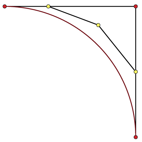
Figure 1.
Circle arc as a formally quartic curve.
The inversion formula is not only helpful to elevate the degree of a parametrisation, but also provides an approximation method for degree reduction.
There are several procedures in the literature for degree reduction. According to [8], degree reduction of a polynomial curve of degree n by another one of lower degree is a special case of polynomial approximation of lower degree. One approach makes use of Chebychev polynomials to obtain the uniform approximation of ; that is, the one for which
is smaller [9,10,11]. The use of dual Bernstein basis is shown in [12].
One could use another norm to minimize the error produced by degree reduction. For instance, any of the norms for ,
In [13], it is shown that the degree reduction that minimizes the error in the norm (least squares approximation) is given by the best Euclidean approximation to the degree-raised control polygon. One of the problems of least squares approximations is that, unless we impose it, the resulting curve does not pass through the first and last vertices of the control polygon [2]. Extensions of the result by [13] to constrained degree reduction are to be found in [14] and to the Jacobi -norm in [15].
A unified approach for degree reduction methods may be found in [16]. Degree reduction for spline curves is discussed in [17,18,19]. An extension to composite curves may be found in [20], considering geometric continuity [21,22,23].
Another approach would be a discrete approximation for which we impose some points on the curve instead of minimizing the distance from the approximating curve to the original curve. For achieving this, we just have to apply the blossom formula to the parametrisation with a degree lower than the actual one.
We must take into account that, although degree reduction is approximating a curve by one of a lower degree, we are conducting a standard Lagrange interpolation of points on the curve by a polynomial curve, with the nice feature of having closed formulas in terms of the parametrisation of the original curve. It has, of course, the same problems as Lagrange interpolation, such as the undesired Runge’s phenomenon when the degree is high; however, it can be managed using standard spline interpolation, for which the previous formulas are also valid.
Some advantages of this procedure are that the approximating curve passes through the endpoints of the original curve and the data are taken symmetrically along the curve. On the contrary, we may lose control of the mean distance to the original curve.
Example 2.
Degree reduction of a polynomial curve parametrised by .
The control polygon for this curve of degree 10 is formed by the points
however, we may reduce the degree to 6 directly with the blossom inverse formula or with the least squares formalism. The results are compared in Figure 2, Figure 3 and Figure 4. The blue curve is the original one and the red curve is the degree-reduced one. The last case corresponds to least squares approximation, but imposing the values of and as the right ones.
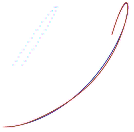
Figure 2.
Degree reduction with blossom inverse formula.
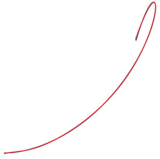
Figure 3.
Degree reduction with least squares formalism.
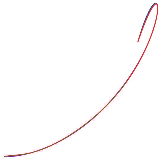
Figure 4.
Degree reduction with least squares formalism, enforcing the first and last vertices.
It is true that the least squares formalism provides a globally closer fitting; however, on the contrary, the blossom inverse formula provides a control polygon that oscillates less and keeps the endpoints of the original one.
The degree reduction procedure need not be applied only to polynomial or rational curves, but can be used for approximating non-algebraic curves. With this procedure the approximating curve passes through the endpoints and is exact for polynomial curves of the same degree.
Example 3.
Approximating curve for the logarithm function, , .
If we approximate with a cubic curve, , with control polygon
the -error committed, ,
is of the same order as the best -cubic approximation, , as can be seen in Figure 5, where the logarithm and the approximating curve are nearly indistinguishable.
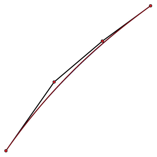
Figure 5.
Approximating curve for the logarithm function.
5. Conclusions
In this paper, a formula that furnishes the blossom of a NURBS parametrisation with no explicit reference to control points, just in terms of points on the NURBS, is provided for all cases of polynomial, rational, NURBS curves and surfaces. The provided solution is not unique, but it is the most symmetric.
It has been shown that this inverse formula may be useful for obtaining control points and weights for any domain of the parametrisation. As applications, it has been used for restricting the domain of a parametrisation, for elevating and reducing its degree and for approximating non-rational parametrisations.
Funding
This research received no external funding.
Data Availability Statement
The original contributions presented in the study are included in the article, further inquiries can be directed to the corresponding author.
Conflicts of Interest
The authors declare no conflict of interest.
References
- de Casteljau, P. Shape Mathematics and CAD; Kogan Page: London, UK, 1986. [Google Scholar]
- Farin, G. Curves and Surfaces for CAGD, 5th ed.; Morgan Kaufmann: San Francisco, CA, USA, 2001. [Google Scholar]
- Ramshaw, L. Blossoms are polar forms. Comput. Aided Geom. Des. 1989, 6, 323–359. [Google Scholar] [CrossRef]
- Seidel, H.-P. A new multiaffine approach to B-splines. Comput. Aided Geom. Des. 1989, 6, 23–32. [Google Scholar] [CrossRef]
- Seidel, H.-P. Knot insertion from a blossoming point of view. Comput. Aided Geom. Des. 1988, 5, 81–86. [Google Scholar] [CrossRef]
- Tuncer, O.O.; Simeonov, P.; Goldman, R. On the uniqueness of the multirational blossom. Comput. Aided Geom. Des. 2023, 107, 102252. [Google Scholar] [CrossRef]
- Farin, G. Triangular Bernstein-Bézier patches. Comput. Aided Geom. Des. 1986, 3, 83–127. [Google Scholar] [CrossRef]
- Farouki, R.T. The Bernstein polynomial basis: A centennial retrospective. Comput. Aided Geometric Des. 2012, 29, 379–419. [Google Scholar] [CrossRef]
- Eck, M. Degree reduction of Bézier curves. Comput. Aided Geom. Des. 1993, 10, 237–252. [Google Scholar]
- Peterson, J. Degree reduction of Bézier curves. Comput.-Aided Des. 1991, 23, 460–461. [Google Scholar]
- Watkins, M.A.; Worsey, A.J. Degree reduction of Bézier curves. Comput.-Aided Des. 1988, 20, 398–405. [Google Scholar] [CrossRef]
- Woźny, P.; Lewanowicz, S. Multi-degree reduction of Bézier curves with constraints, using dual Bernstein basis polynomials. Comput. Aided Geometric Des. 2009, 26, 566–579. [Google Scholar] [CrossRef]
- Lutterkort, D.; Peters, J.; Reif, U. Polynomial degree reduction in the L2-norm equals best Euclidean approximation of Bézier coefficients. Comput. Aided Geom. Des. 2000, 16, 607–612. [Google Scholar] [CrossRef]
- Ahn, Y.J.; Lee, B.; Park, Y.; Yoo, J. Constrained polynomial degree reduction in the L2-norm equals best weighted Euclidean approximation of Bézier coefficients. Comput. Aided Geom. Des. 2004, 21, 181–191. [Google Scholar] [CrossRef]
- Ait-Haddou, R.; Bartoň, M. Constrained multi-degree reduction with respect to Jacobi norms. Comput. Aided Geom. Des. 2016, 42, 23–30. [Google Scholar] [CrossRef]
- Szafnicki, B. A unified approach for degree reduction of polynomials in the Bernstein basis. Part I: Real polynomials. J. Comput. Appl. Math. 2002, 142, 287–312. [Google Scholar] [CrossRef]
- Piegl, L.; Tiller, W. Algorithm for degree reduction of B-spline curves. Comput. Aided Design 1995, 27, 101–110. [Google Scholar] [CrossRef]
- Wolters, H.; Wu, G.; Farin, G. Degree reduction of B-spline curves. In Geometric Modelling; Farin, G., Bieri, H., Brunnett, G., DeRose, T., Eds.; Springer: Berlin/Heidelberg, Germany, 1998. [Google Scholar]
- Yong, J.; Hu, S.; Sun, J.; Tan, X. Degree reduction of B-spline curves. Comput. Aided Geometric Des. 2001, 18, 117–128. [Google Scholar] [CrossRef]
- Gospodarczyk, P.; Lewanowicz, S.; Woźny, P. Degree reduction of composite Bézier curves. Appl. Math. Comput. 2017, 293, 40–48. [Google Scholar] [CrossRef]
- Lu, L. Explicit G2-constrained degree reduction of Bézier curves by quadratic optimization. J. Comput. Appl. Math. 2013, 253, 80–88. [Google Scholar] [CrossRef]
- Lu, L.; Wang, G. Optimal multi-degree reduction of Bézier curves with G2-continuity. Comput. Geom. Des. 2006, 23, 673–683. [Google Scholar] [CrossRef]
- Rababah, A.; Mann, S. Linear methods for G1, G2 and G3—Multi-degree reduction of Bézier curves. Comput.-Aided Des. 2013, 45, 405–414. [Google Scholar] [CrossRef]
Disclaimer/Publisher’s Note: The statements, opinions and data contained in all publications are solely those of the individual author(s) and contributor(s) and not of MDPI and/or the editor(s). MDPI and/or the editor(s) disclaim responsibility for any injury to people or property resulting from any ideas, methods, instructions or products referred to in the content. |
© 2024 by the author. Licensee MDPI, Basel, Switzerland. This article is an open access article distributed under the terms and conditions of the Creative Commons Attribution (CC BY) license (https://creativecommons.org/licenses/by/4.0/).