
Sharma–Taneja–Mittal Entropy and Its Application of Obesity in Saudi Arabia


Abstract
1. Introduction
Work Motivation
2. The Nonparametric Estimators Proposed
2.1. First and Second Procedures
- From (4), the Vasicek’s estimator is available for our utilization to estimate the Sharma–Taneja–Mittal entropy measure as
2.2. Third Procedure
2.3. Fourth Procedure
3. Numerical Study
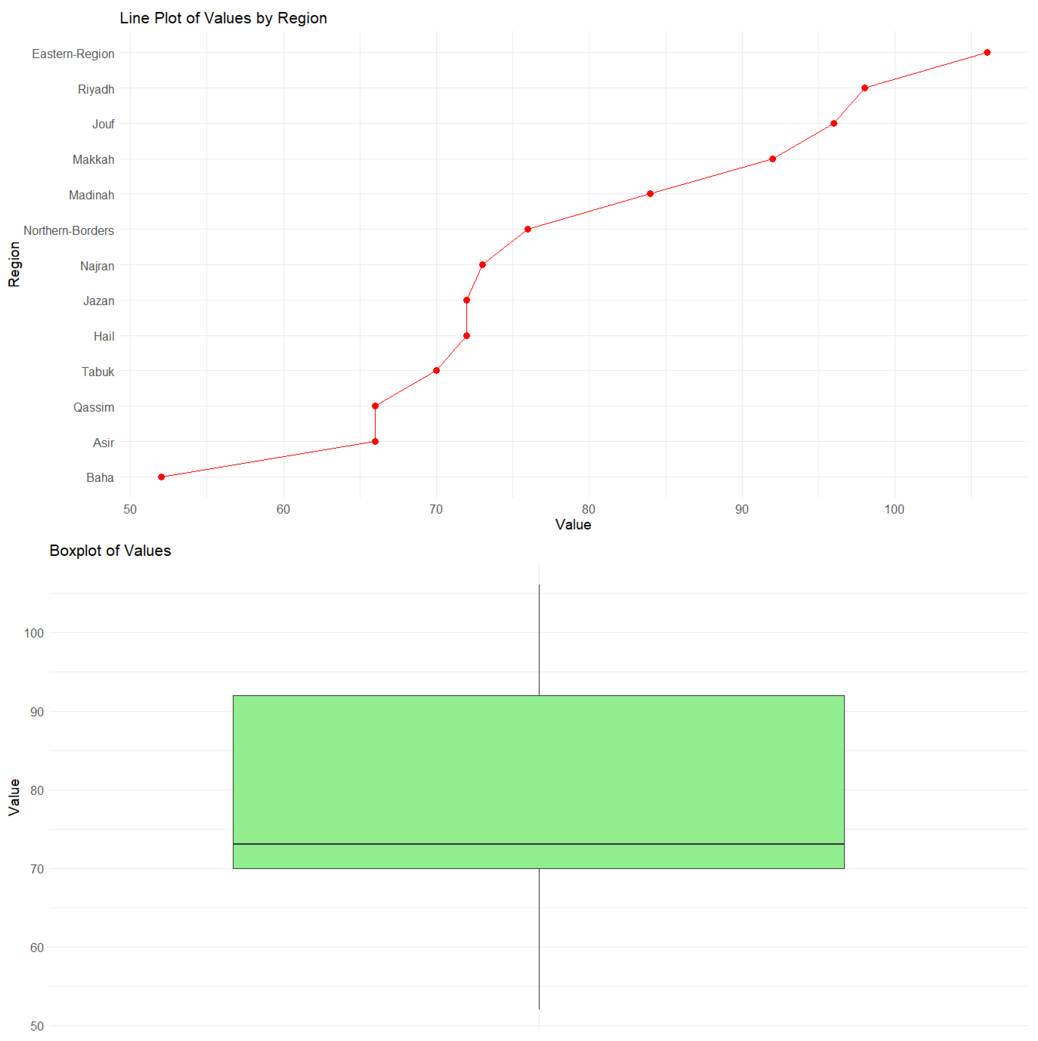
3.1. Real Data
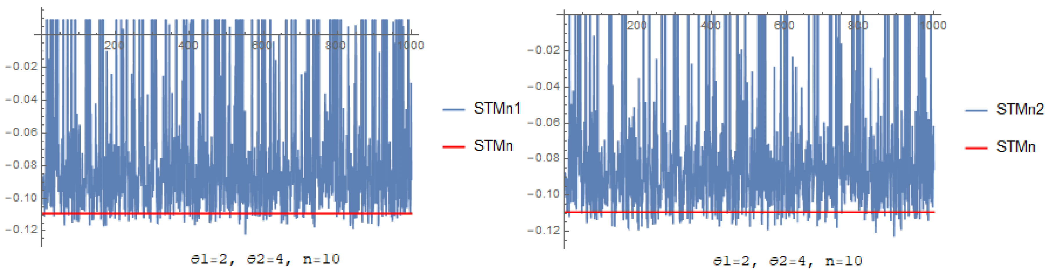
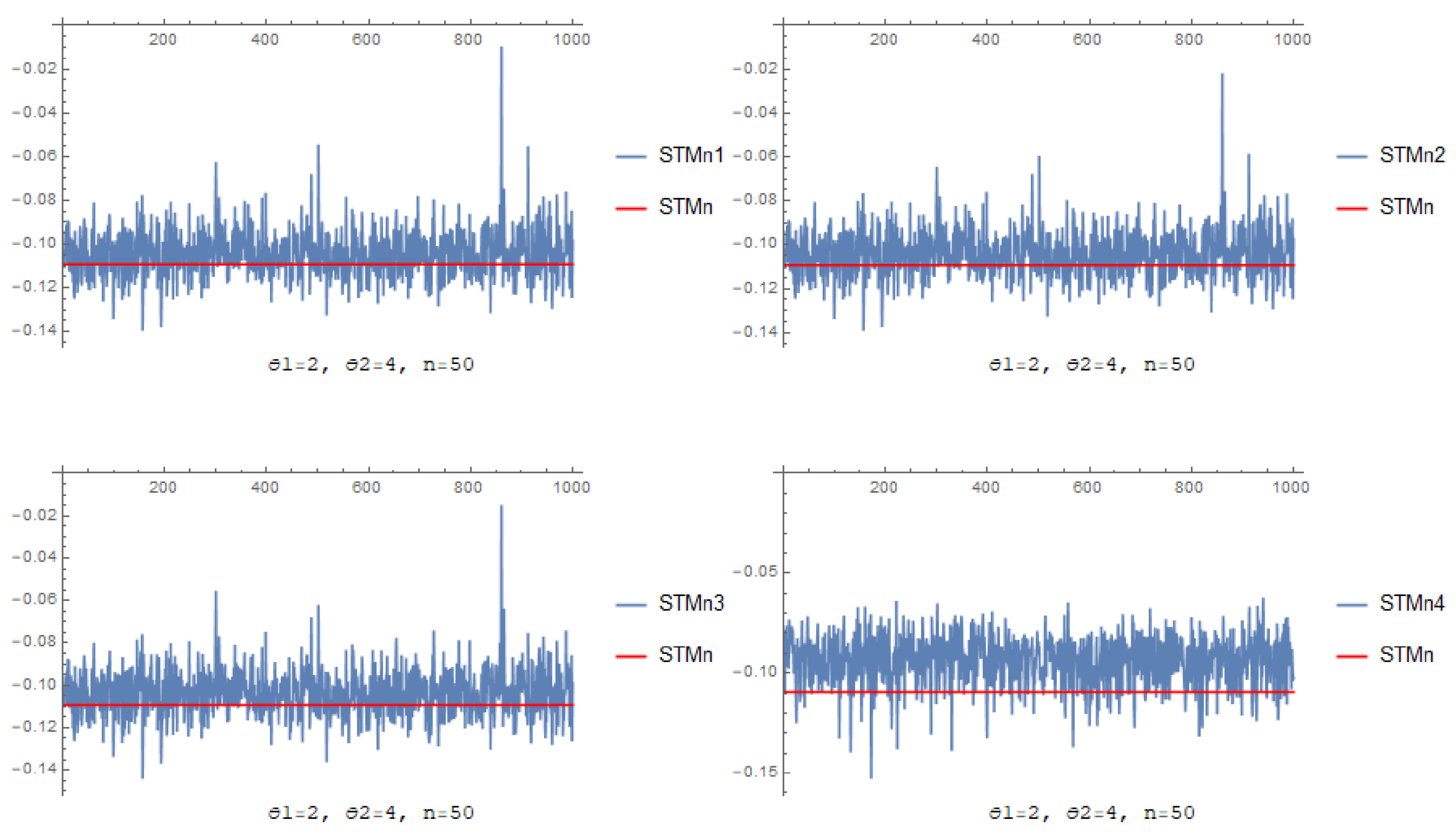
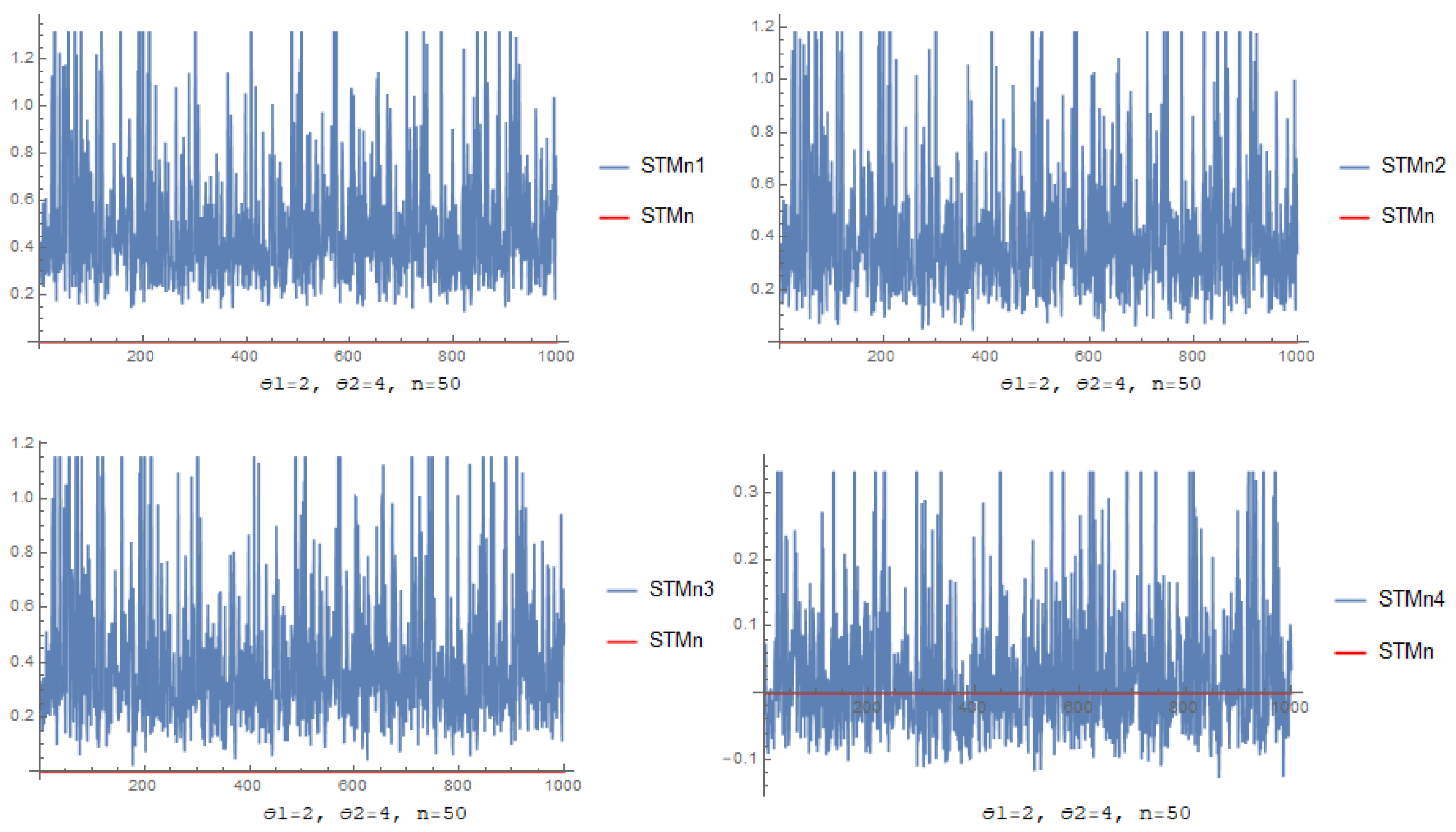
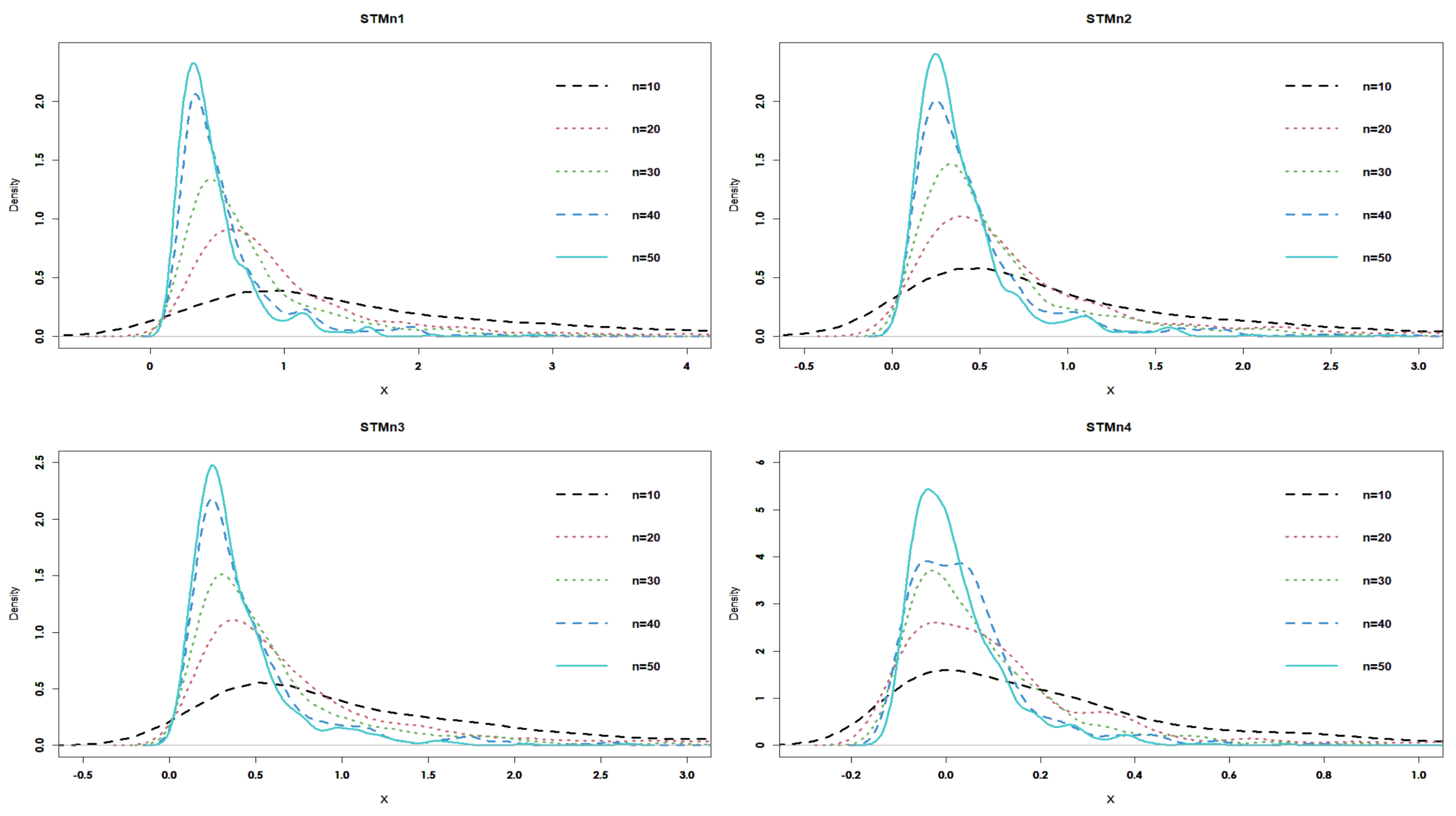
3.2. Investigation through Simulation
- Through increasing n, the and its corresponding decreases for each estimator.
4. Test Statistic of Testing Uniformity
Critical Values and Power Comparisons
- In increasing the sample size n, the difference in percentage points decreases.
- For fixed n and increasing and , the difference in percentage points increases.
- The fourth estimator introduces the percentage points that cover the actual value of the Sharma–Taneja–Mittal entropy measure for the different values of , , and n.
- Cramer–von Mises test statistic:
- Kolmogrov–Smirnov test statistic:
- Anderson–Darling test statistic:
- Extropy test statistic:where the positive integer window size ; if and if ; and is defined in (10).
- Under alternative , the four Sharma–Taneja–Mittal entropy estimators have good behavior compared with the other tests. Stephens [29] viewed alternative as indicating a shift in the mean, alternative as signifying a move toward a smaller variance, and alternative as representing a shift toward a larger variance. Therefore, our tests perform optimally compared to alternatives when there is a shift toward a smaller variance.
- Under alternatives , , and , the fourth estimator, which relies on the kernel function, outperforms all other tests across various values of n, , and .
- For fixed n and increasing and , the power of the four Sharma–Taneja–Mittal entropy estimators decreases.
5. Classification Problem via Pattern Recognition
6. Conclusions
Author Contributions
Funding
Data Availability Statement
Acknowledgments
Conflicts of Interest
References
- Shannon, C. A mathematical theory of communication. Bell Syst. Tech. J. 1948, 27, 379–423. [Google Scholar] [CrossRef]
- Rao, M.; Chen, Y.; Vemuri, B.; Wang, F. Cumulative residual entropy: A new measure of information. IEEE Trans. Inf. Theory 2004, 50, 1220–1228. [Google Scholar] [CrossRef]
- Tsallis, C. Possible generalization of Boltzmann-Gibbs statistics. J. Stat. Phys. 1988, 52, 479–487. [Google Scholar] [CrossRef]
- Sharma, B.D.; Taneja, I.J. Entropy of type (α,β) and other generalized measures in information theory. Metrika 1975, 22, 205–215. [Google Scholar] [CrossRef]
- Mittal, D.P. On some functional equations concerning entropy, directed divergence and inaccuracy. Metrika 1975, 22, 35–45. [Google Scholar] [CrossRef]
- Kattumannil, S.K.; Sreedevi, E.P.; Balakrishnan, N. A Generalized Measure of Cumulative Residual Entropy. Entropy 2022, 24, 444. [Google Scholar] [CrossRef]
- Sudheesh, K.K.; Sreedevi, E.P.; Balakrishnan, N. Relationships between cumulative entropy/extropy, Gini mean difference and probability weighted moments. Probab. Eng. Inf. Sci. 2024, 38, 28–38. [Google Scholar]
- Vasicek, O. A Test for Normality based on Sample Entropy. J. R. Stat. Soc.-Ser. 1976, 38, 54–59. [Google Scholar] [CrossRef]
- Ebrahimi, N.; Pflughoeft, K.; Soofi, E.S. Two Measures of Sample Entropy. Stat. Probab. Lett. 1994, 20, 225–234. [Google Scholar] [CrossRef]
- Noughabi, H.A.; Jarrahiferiz, J. Extropy of order statistics applied to testing symmetry. Commun. Stat.-Simul. 2020, 51, 3389–3399. [Google Scholar] [CrossRef]
- Qiu, G.; Jia, K. Extropy Estimators with Applications in Testing Uniformity. J. Nonparametric Stat. 2018, 30, 182–196. [Google Scholar] [CrossRef]
- Wachowiak, M.P.; Smolikova, R.; Tourassi, G.D.; Elmaghraby, A.S. Estimation of generalized entropies with sample spacing. Pattern Anal. Appl. 2005, 8, 95–101. [Google Scholar] [CrossRef]
- Wanke, P. The uniform distribution as a first practical approach to new product inventory management. Int. J. Prod. Econ. 2008, 114, 811–819. [Google Scholar] [CrossRef]
- Correa, J.C. A new Estimator of entropy. Commun. Stat.-Theory Methods 1995, 24, 2439–2449. [Google Scholar] [CrossRef]
- Parzen, E. On estimation of a probability density function and mode. Ann. Math. Stat. 1962, 33, 1065–1076. [Google Scholar] [CrossRef]
- Masry, E. Recursive probability density estimation for weakly dependent stationary processes. IEEE Trans. Inf. Theory 1986, 32, 254–267. [Google Scholar] [CrossRef]
- Grzegorzewski, P.; Wieczorkowski, R. Entropy-based Goodness-of-fit Test for Exponentiality. Commun. Stat.-Theory Methods 1999, 28, 1183–1202. [Google Scholar] [CrossRef]
- Althumiri, N.A.; Basyouni, M.H.; AlMousa, N.; AlJuwaysim, M.F.; Almubark, R.A.; BinDhim, N.F.; Alkhamaali, Z.; Alqahtani, S.A. Obesity in Saudi Arabia in 2020: Prevalence, Distribution, and Its Current Association with Various Health Conditions. Healthcare 2021, 9, 311. [Google Scholar] [CrossRef]
- Mudholkar, G.S.; Tian, L. An Entropy Characterization of the Inverse Gaussian Distribution and Related Goodness-of-Fit Test. J. Stat. Plan. Inference 2002, 102, 211–221. [Google Scholar] [CrossRef]
- Marhuenda, Y.; Morales, D.; Pardo, M.C. A Comparison of Uniformity Tests. Statistics 2005, 39, 315–327. [Google Scholar] [CrossRef]
- Dudewicz, E.J.; Van der Meulen, E.C. Entropy-based Tests of Uniformity. J. Am. Stat. Assoc. 1981, 76, 967–974. [Google Scholar] [CrossRef]
- Zamanzade, E.; Arghami, N.R. Goodness-of-Fit Test based on Correcting Moments of Modified Entropy Estimator. J. Stat. Comput. Simul. 2011, 81, 2077–2093. [Google Scholar] [CrossRef]
- Zamanzade, E. Testing Uniformity based on New Entropy Estimators. J. Stat. Simul. 2015, 85, 3191–3205. [Google Scholar] [CrossRef]
- Cramér, H. On the Composition of Elementary Errors: II. Statistical Applications. Scand. Actuar. J. 1928, 1928, 141–180. [Google Scholar]
- Von Mises, R. Wahrscheinlichkeitsrechnung und ihre Anwendung in der Statistik und Theoretischen Physik; Deuticke: Leipzig, Germany, 1931. [Google Scholar]
- Kolmogorov, A.N. Sulla Determinazione Empirica di una Legge di Distibuziane. G. Dell’IstitutaItaliano Degli Attuari 1933, 4, 83–91. [Google Scholar]
- Smirnov, N.V. Estimate of Derivation between Empirical Distribution Functions in Two Independent Samples. Bull. Mosc. Univ. 1939, 2, 3–16. (In Russian) [Google Scholar]
- Anderson, T.W.; Darling, D.A. A Test of Goodness-of-Fit. J. Am. Stat. Assoc. 1954, 49, 765–769. [Google Scholar] [CrossRef]
- Stephens, M.A. EDF statistics for goodness of fit and some comparisons. J. Am. Stat. Assoc. 1974, 69, 730–737. [Google Scholar] [CrossRef]
- Fisher, R.A. Iris. UCI Machine Learning Repository. 1988. Available online: https://archive.ics.uci.edu/dataset/53/iris (accessed on 1 July 2024).
- Kang, B.Y.; Li, Y.; Deng, Y.; Zhang, Y.J.; Deng, X.Y. Determination of basic probability assignment based on interval numbers and its application. Dianzi Xuebao (Acta Electron. Sin.) 2012, 40, 1092–1096. [Google Scholar]
- Buono, F.; Longobardi, M. A dual measure of uncertainty: The deng extropy. Entropy 2020, 22, 582. [Google Scholar] [CrossRef]


| Distributions | ||
|---|---|---|
| Standard uniform | y; | 0 |
| Uniform | ; | |
| Exponential | ; , | |
| Power | ; , | |
| Pareto I | ; , |
| STMn | STMn1 | STMn2 | STMn3 | STMn4 | |
|---|---|---|---|---|---|
| 1, 2 | −0.981514 | −0.9877 0.006215 −0.63325 | −0.98859 0.00708 −0.7218 | −0.98611 0.004604 −0.46912 | −0.982392 0.000878187 −0.0894727 |
| 1, 3 | −0.499803 | −0.499781 | −0.499851 | −0.499853 | −0.49983 |
| 2, 3 | −0.0180914 | −0.011832 | −0.0111024 | −0.013587 | −0.017268 |
| 2, 4 | −0.00923853 | −0.00613189 | −0.00569784 | −0.00693782 | −0.00880043 |
| 3, 4 | −0.000385664 | −0.00043179 | −0.000293323 | −0.000288458 | −0.000332904 |
| 3, 5 | −0.000197194 | −0.000219139 | −0.000149047 | −0.000147068 | −0.000169846 |
| 3, 6 | −0.000131531 | −0.000146162 | −0.0000994011 | −0.0000980839 | −0.000113278 |
| , | ||||
|---|---|---|---|---|
| n | STMn1 | STMn2 | STMn3 | STMn4 |
| 10 | 0.14461 (0.132534) | 0.129365 (0.124113) | 0.129513 (0.122418) | 0.0855713 (0.0847806) |
| 20 | 0.0816596 (0.0754353) | 0.0781294 (0.0743387) | 0.0734482 (0.0714015) | 0.0671174 (0.0542884) |
| 30 | 0.0665794 (0.0616712) | 0.0648844 (0.0613456) | 0.0607927 (0.0591587) | 0.0626705 (0.0418085) |
| 40 | 0.0548361 (0.0516832) | 0.0539021 (0.0515542) | 0.051165 (0.0502906) | 0.0611906 (0.033919) |
| 50 | 0.0469785 (0.0450095) | 0.0464326 (0.044974) | 0.0444812 (0.0440465) | 0.0608884 (0.030506) |
| , | ||||
| 10 | 0.16812 (0.150558) | 0.132232 (0.121322) | 0.124813 (0.115287) | 0.0277982 (0.0264395) |
| 20 | 0.0549721 (0.0462316) | 0.0505812 (0.043901) | 0.0446313 (0.0403246) | 0.0219168 (0.0143902) |
| 30 | 0.0408954 (0.0342019) | 0.0389946 (0.0333485) | 0.0346193 (0.031104) | 0.0210433 (0.0103421) |
| 40 | 0.0314564 (0.0265216) | 0.0304197 (0.0261155) | 0.0273505 (0.0248309) | 0.0208732 (0.00797974) |
| 50 | 0.0258993 (0.0221422) | 0.025241 (0.0219065) | 0.0229246 (0.0210369) | 0.0208521 (0.00721379) |
| , | ||||
|---|---|---|---|---|
| n | STMn1 | STMn2 | STMn3 | STMn4 |
| 10 | 0.212645 (0.191847) | 0.156784 (0.140966) | 0.144111 (0.13389) | 0.0358821 (0.0355005) |
| 20 | 0.0421057 (0.0312879) | 0.0384475 (0.0281834) | 0.0342259 (0.0270588) | 0.0275815 (0.0268353) |
| 30 | 0.0285834 (0.0206948) | 0.0275623 (0.0197346) | 0.0258025 (0.0199804) | 0.0239704 (0.0217743) |
| 40 | 0.0214715 (0.0148946) | 0.0212414 (0.0146132) | 0.0202013 (0.0150943) | 0.0220457 (0.0182628) |
| 50 | 0.0181633 (0.0122971) | 0.0181706 (0.0121897) | 0.017365 (0.0126431) | 0.0212449 (0.0163526) |
| , | ||||
| 10 | 0.385437 (0.377294) | 0.257659 (0.251518) | 0.252319 (0.247595) | 0.0297265 (0.0297261) |
| 20 | 0.0377388 (0.035082) | 0.0320088 (0.0291091) | 0.0306848 (0.0283813) | 0.0237941 (0.0212249) |
| 30 | 0.0217646 (0.0199784) | 0.0204595 (0.01847) | 0.0205809 (0.0187179) | 0.0216616 (0.0169128) |
| 40 | 0.0146617 (0.0133615) | 0.0144534 (0.0129698) | 0.0148408 (0.0132896) | 0.020708 (0.0140194) |
| 50 | 0.0121171 (0.0110248) | 0.0120924 (0.0108211) | 0.0125347 (0.0111286) | 0.0203776 (0.0125835) |
| n | STMn1 | STMn2 | STMn3 | STMn4 |
| 10 | 0.324999 (0.302211) | 0.288194 (0.288029) | 0.33933 (0.301435) | 0.257691 (0.233468) |
| 20 | 0.187321 (0.160289) | 0.163991 (0.160743) | 0.175266 (0.158899) | 0.137397 (0.136884) |
| 30 | 0.141005 (0.118538) | 0.124708 (0.121589) | 0.1305 (0.119432) | 0.100954 (0.0994799) |
| 40 | 0.104646 (0.0893122) | 0.0935664 (0.0925936) | 0.0982116 (0.0919585) | 0.0858848 (0.0791714) |
| 50 | 0.08443 (0.0737325) | 0.0767405 (0.0766393) | 0.0800848 (0.0760987) | 0.0790904 (0.0671044) |
| 10 | 1.75955 (1.42486) | 1.21433 (1.06603) | 1.19997 (1.0179) | 0.366708 (0.322417) |
| 20 | 0.58992 (0.363632) | 0.46281 (0.336973) | 0.450122 (0.319156) | 0.17617 (0.169084) |
| 30 | 0.418685 (0.243132) | 0.344598 (0.239065) | 0.331397 (0.224744) | 0.120857 (0.120316) |
| 40 | 0.307888 (0.158279) | 0.250952 (0.159762) | 0.243638 (0.151957) | 0.0930044 (0.0927536) |
| 50 | 0.25518 (0.123582) | 0.206611 (0.126006) | 0.203724 (0.12069) | 0.0807951 (0.0788088) |
| n | STMn1 | STMn2 | STMn3 | STMn4 |
| 10 | 3.24246 (2.59429) | 2.2065 (1.88305) | 2.09309 (1.77137) | 0.480594 (0.416191) |
| 20 | 1.0107 (0.573765) | 0.795043 (0.519611) | 0.744272 (0.48933) | 0.22101 (0.203322) |
| 30 | 0.711141 (0.373241) | 0.591952 (0.36185) | 0.5504 (0.337942) | 0.148635 (0.142783) |
| 40 | 0.526556 (0.230126) | 0.438324 (0.229652) | 0.408419 (0.216469) | 0.108955 (0.107423) |
| 50 | 0.441826 (0.175791) | 0.368536 (0.177629) | 0.347178 (0.169075) | 0.0916764 (0.0915285) |
| 10 | 12.7007 (12.2844) | 9.39012 (9.16204) | 8.66346 (8.36002) | 0.711518 (0.625726) |
| 20 | 1.81269 (1.39144) | 1.49908 (1.20588) | 1.44436 (1.15244) | 0.293881 (0.264811) |
| 30 | 1.16698 (0.841139) | 1.03401 (0.793981) | 0.98455 (0.749115) | 0.193146 (0.180129) |
| 40 | 0.722116 (0.416834) | 0.640433 (0.411796) | 0.617659 (0.395966) | 0.135057 (0.128615) |
| 50 | 0.57095 (0.295466) | 0.505213 (0.295314) | 0.494735 (0.28746) | 0.113137 (0.110129) |
| STMn1 | STMn2 | STMn3 | STMn4 | |
| 1, 2 | (−0.252703, 0.560403) | (−0.343895, 0.419436) | (−0.259882, 0.526772) | (−0.202206, 0.406931) |
| 1, 3 | (0.141055, 2.52503) | (−0.0899544, 1.67325) | (−0.0777993, 1.68698) | (−0.170763, 0.572097) |
| 2, 3 | (0.526473, 4.53774) | (0.15415, 2.98353) | (0.0929531, 2.8155) | (−0.141173, 0.776607) |
| 2, 4 | (0.264779, 9.23515) | (0.0310672, 6.0256) | (0.0588096, 6.21605) | (−0.124758, 1.02762) |
| 1, 2 | (−0.127013, 0.46065) | (−0.197468, 0.385614) | (−0.17302, 0.41996) | (−0.160847, 0.23215) |
| 1, 3 | (0.0780801, 1.33191) | (−0.0457253, 1.13025) | (−0.0456312, 1.05308) | (−0.138835, 0.343722) |
| 2, 3 | (0.276409, 2.21915) | (0.105258, 1.87488) | (0.0781993, 1.68431) | (−0.118179, 0.442431) |
| 2, 4 | (0.212467, 4.06039) | (0.0764948, 3.60973) | (0.0763925, 3.17668) | (−0.104545, 0.567234) |
| 1, 2 | (−0.0937319, 0.332303) | (−0.152613, 0.293168) | (−0.131898, 0.302147) | (−0.150464, 0.140867) |
| 1, 3 | (0.0654442, 0.862308) | (−0.023163, 0.772293) | (−0.0217618, 0.729274) | (−0.129833, 0.224846) |
| 2, 3 | (0.224547, 1.43339) | (0.0999416, 1.27472) | (0.0825614, 1.16331) | (−0.111212, 0.29924) |
| 2, 4 | (0.19284, 2.4853) | (0.0881774, 2.27333) | (0.0800395, 2.03479) | (−0.0994638, 0.387009) |
| n | Alt. | ||||||||
|---|---|---|---|---|---|---|---|---|---|
| 10 | 0.242 | 0.253 | 0.248 | 0.255 | 0.154 | 0.156 | 0.168 | 0.136 | |
| 0.464 | 0.483 | 0.471 | 0.508 | 0.386 | 0.409 | 0.438 | 0.32 | ||
| 0.225 | 0.243 | 0.266 | 0.252 | 0.037 | 0.015 | 0.026 | 0.21 | ||
| 0.494 | 0.645 | 0.554 | 0.499 | 0.044 | 0.009 | 0.022 | 0.455 | ||
| 0.876 | 0.948 | 0.897 | 0.823 | 0.087 | 0.018 | 0.051 | 0.801 | ||
| 0.088 | 0.102 | 0.108 | 0.091 | 0.113 | 0.121 | 0.098 | 0.082 | ||
| 0.139 | 0.172 | 0.241 | 0.823 | 0.199 | 0.227 | 0.155 | 0.131 | ||
| 20 | 0.183 | 0.204 | 0.175 | 0.500 | 0.279 | 0.309 | 0.324 | 0.258 | |
| 0.521 | 0.554 | 0.487 | 0.833 | 0.699 | 0.756 | 0.771 | 0.665 | ||
| 0.237 | 0.253 | 0.269 | 0.567 | 0.059 | 0.032 | 0.042 | 0.399 | ||
| 0.649 | 0.754 | 0.663 | 0.888 | 0.125 | 0.092 | 0.100 | 0.808 | ||
| 0.988 | 0.995 | 0.986 | 1.000 | 0.410 | 0.537 | 0.513 | 0.991 | ||
| 0.059 | 0.061 | 0.072 | 0.077 | 0.150 | 0.156 | 0.119 | 0.155 | ||
| 0.100 | 0.093 | 0.115 | 1.000 | 0.315 | 0.371 | 0.250 | 0.363 | ||
| 30 | 0.266 | 0.271 | 0.260 | 0.701 | 0.520 | 0.592 | 0.594 | 0.529 | |
| 0.737 | 0.740 | 0.712 | 0.966 | 0.955 | 0.978 | 0.978 | 0.919 | ||
| 0.358 | 0.345 | 0.374 | 0.786 | 0.113 | 0.108 | 0.093 | 0.581 | ||
| 0.873 | 0.917 | 0.879 | 0.989 | 0.376 | 0.560 | 0.445 | 0.924 | ||
| 1.000 | 1.000 | 1.000 | 1.000 | 0.928 | 0.996 | 0.986 | 1 | ||
| 0.063 | 0.063 | 0.088 | 0.071 | 0.230 | 0.241 | 0.175 | 0.217 | ||
| 0.177 | 0.128 | 0.154 | 1.000 | 0.561 | 0.695 | 0.557 | 0.782 | ||
| n | Alt. | ||||||||
|---|---|---|---|---|---|---|---|---|---|
| 10 | 0.146 | 0.185 | 0.174 | 0.22 | 0.154 | 0.156 | 0.168 | 0.136 | |
| 0.332 | 0.376 | 0.358 | 0.437 | 0.386 | 0.409 | 0.438 | 0.32 | ||
| 0.177 | 0.18 | 0.187 | 0.213 | 0.037 | 0.015 | 0.026 | 0.21 | ||
| 0.403 | 0.663 | 0.415 | 0.443 | 0.044 | 0.009 | 0.022 | 0.455 | ||
| 0.82 | 0.963 | 0.806 | 0.762 | 0.087 | 0.018 | 0.051 | 0.801 | ||
| 0.097 | 0.128 | 0.093 | 0.096 | 0.113 | 0.121 | 0.098 | 0.082 | ||
| 0.165 | 0.201 | 0.191 | 0.762 | 0.199 | 0.227 | 0.155 | 0.131 | ||
| 20 | 0.129 | 0.148 | 0.127 | 0.399 | 0.279 | 0.309 | 0.324 | 0.258 | |
| 0.419 | 0.435 | 0.416 | 0.74 | 0.699 | 0.756 | 0.771 | 0.665 | ||
| 0.174 | 0.174 | 0.177 | 0.447 | 0.059 | 0.032 | 0.042 | 0.399 | ||
| 0.53 | 0.649 | 0.522 | 0.826 | 0.125 | 0.092 | 0.1 | 0.808 | ||
| 0.967 | 0.988 | 0.956 | 0.996 | 0.410 | 0.537 | 0.513 | 0.991 | ||
| 0.072 | 0.072 | 0.085 | 0.078 | 0.150 | 0.156 | 0.119 | 0.155 | ||
| 0.128 | 0.117 | 0.146 | 0.996 | 0.315 | 0.371 | 0.25 | 0.363 | ||
| 30 | 0.22 | 0.222 | 0.202 | 0.566 | 0.520 | 0.592 | 0.594 | 0.529 | |
| 0.627 | 0.639 | 0.595 | 0.928 | 0.955 | 0.978 | 0.978 | 0.919 | ||
| 0.279 | 0.273 | 0.266 | 0.68 | 0.113 | 0.108 | 0.093 | 0.581 | ||
| 0.779 | 0.845 | 0.745 | 0.97 | 0.376 | 0.560 | 0.445 | 0.924 | ||
| 0.998 | 1 | 0.993 | 1 | 0.928 | 0.996 | 0.986 | 1 | ||
| 0.101 | 0.09 | 0.108 | 0.07 | 0.230 | 0.241 | 0.175 | 0.217 | ||
| 0.249 | 0.186 | 0.244 | 1 | 0.561 | 0.695 | 0.557 | 0.782 | ||
| n | Alt. | ||||||||
|---|---|---|---|---|---|---|---|---|---|
| 10 | 0.135 | 0.162 | 0.157 | 0.181 | 0.154 | 0.156 | 0.168 | 0.136 | |
| 0.31 | 0.354 | 0.342 | 0.368 | 0.386 | 0.409 | 0.438 | 0.32 | ||
| 0.169 | 0.172 | 0.176 | 0.175 | 0.037 | 0.015 | 0.026 | 0.21 | ||
| 0.384 | 0.673 | 0.382 | 0.366 | 0.044 | 0.009 | 0.022 | 0.455 | ||
| 0.806 | 0.965 | 0.787 | 0.692 | 0.087 | 0.018 | 0.051 | 0.801 | ||
| 0.099 | 0.129 | 0.092 | 0.091 | 0.113 | 0.121 | 0.098 | 0.082 | ||
| 0.162 | 0.205 | 0.178 | 0.943 | 0.199 | 0.227 | 0.155 | 0.131 | ||
| 20 | 0.121 | 0.134 | 0.126 | 0.356 | 0.279 | 0.309 | 0.324 | 0.258 | |
| 0.388 | 0.407 | 0.388 | 0.71 | 0.699 | 0.756 | 0.771 | 0.665 | ||
| 0.157 | 0.159 | 0.161 | 0.407 | 0.059 | 0.032 | 0.042 | 0.399 | ||
| 0.492 | 0.649 | 0.465 | 0.793 | 0.125 | 0.092 | 0.1 | 0.808 | ||
| 0.955 | 0.985 | 0.938 | 0.993 | 0.410 | 0.537 | 0.513 | 0.991 | ||
| 0.078 | 0.074 | 0.089 | 0.084 | 0.150 | 0.156 | 0.119 | 0.155 | ||
| 0.139 | 0.12 | 0.161 | 1 | 0.315 | 0.371 | 0.25 | 0.363 | ||
| 30 | 0.189 | 0.211 | 0.185 | 0.509 | 0.520 | 0.592 | 0.594 | 0.529 | |
| 0.575 | 0.586 | 0.554 | 0.894 | 0.955 | 0.978 | 0.978 | 0.919 | ||
| 0.246 | 0.234 | 0.229 | 0.635 | 0.113 | 0.108 | 0.093 | 0.581 | ||
| 0.718 | 0.825 | 0.692 | 0.958 | 0.376 | 0.560 | 0.445 | 0.924 | ||
| 0.995 | 0.999 | 0.99 | 1 | 0.928 | 0.996 | 0.986 | 1 | ||
| 0.106 | 0.094 | 0.112 | 0.072 | 0.230 | 0.241 | 0.175 | 0.217 | ||
| 0.257 | 0.201 | 0.275 | 1 | 0.561 | 0.695 | 0.557 | 0.782 | ||
| n | Alt. | ||||||||
|---|---|---|---|---|---|---|---|---|---|
| 10 | 0.133 | 0.152 | 0.137 | 0.179 | 0.154 | 0.156 | 0.168 | 0.136 | |
| 0.292 | 0.325 | 0.307 | 0.357 | 0.386 | 0.409 | 0.438 | 0.32 | ||
| 0.129 | 0.144 | 0.141 | 0.173 | 0.037 | 0.015 | 0.026 | 0.21 | ||
| 0.288 | 0.455 | 0.318 | 0.364 | 0.044 | 0.009 | 0.022 | 0.455 | ||
| 0.684 | 0.832 | 0.712 | 0.68 | 0.087 | 0.018 | 0.051 | 0.801 | ||
| 0.096 | 0.116 | 0.097 | 0.095 | 0.113 | 0.121 | 0.098 | 0.082 | ||
| 0.163 | 0.186 | 0.179 | 0.802 | 0.199 | 0.227 | 0.155 | 0.131 | ||
| 20 | 0.118 | 0.118 | 0.118 | 0.338 | 0.279 | 0.309 | 0.324 | 0.258 | |
| 0.351 | 0.347 | 0.344 | 0.693 | 0.699 | 0.756 | 0.771 | 0.665 | ||
| 0.135 | 0.135 | 0.144 | 0.399 | 0.059 | 0.032 | 0.042 | 0.399 | ||
| 0.401 | 0.475 | 0.396 | 0.779 | 0.125 | 0.092 | 0.1 | 0.808 | ||
| 0.897 | 0.939 | 0.892 | 0.991 | 0.410 | 0.537 | 0.513 | 0.991 | ||
| 0.084 | 0.082 | 0.097 | 0.091 | 0.150 | 0.156 | 0.119 | 0.155 | ||
| 0.185 | 0.127 | 0.182 | 1 | 0.315 | 0.371 | 0.25 | 0.363 | ||
| 30 | 0.164 | 0.176 | 0.165 | 0.476 | 0.520 | 0.592 | 0.594 | 0.529 | |
| 0.495 | 0.509 | 0.484 | 0.871 | 0.955 | 0.978 | 0.978 | 0.919 | ||
| 0.177 | 0.191 | 0.195 | 0.606 | 0.113 | 0.108 | 0.093 | 0.581 | ||
| 0.611 | 0.664 | 0.592 | 0.947 | 0.376 | 0.560 | 0.445 | 0.924 | ||
| 0.984 | 0.99 | 0.983 | 1 | 0.928 | 0.996 | 0.986 | 1 | ||
| 0.11 | 0.099 | 0.117 | 0.074 | 0.230 | 0.241 | 0.175 | 0.217 | ||
| 0.3 | 0.216 | 0.284 | 1 | 0.561 | 0.695 | 0.557 | 0.782 | ||
| (i) Item | ||||
|---|---|---|---|---|
| [4.4, 5.8] | [2.3, 4.4] | [1.0, 1.9] | [0.1, 0.6] | |
| [4.9, 7.0] | [2.0, 3.4] | [3.0, 5.1] | [1.0, 1.7] | |
| [4.9, 7.9] | [2.2, 3.8] | [4.5, 6.9] | [1.4, 2.5] | |
| (ii) Item | ||||
| P() | 0.270571 | 0.27477 | 0.145978 | 0.156327 |
| P() | 0.419584 | 0.351607 | 0.429446 | 0.373669 |
| P() | 0.309845 | 0.373622 | 0.424576 | 0.470003 |
| (i) Item | ||||
|---|---|---|---|---|
| , | −0.654737 | −0.66128 | −0.614002 | −0.61503 |
| , | −0.438289 | −0.441816 | −0.420576 | −0.42009 |
| , | −0.221841 | −0.222352 | −0.227151 | −0.22515 |
| , | −0.149847 | −0.149125 | −0.159518 | −0.158039 |
| (ii) Item | ||||
| , | 0.254601 | 0.256272 | 0.244438 | 0.244689 |
| , | 0.25202 | 0.25291 | 0.247595 | 0.247475 |
| , | 0.249429 | 0.249557 | 0.250758 | 0.250256 |
| , | 0.248928 | 0.248749 | 0.251347 | 0.250976 |
| Approach | Overall | |||
|---|---|---|---|---|
| Kang’s approach | 100% | 96% | 84% | 93.33% |
| Buono and Longobardi’s approach | 100% | 96% | 86% | 94% |
| Sharma–Taneja–Mittal approach | 100% | 98% | 86% | 94.66% |
Disclaimer/Publisher’s Note: The statements, opinions and data contained in all publications are solely those of the individual author(s) and contributor(s) and not of MDPI and/or the editor(s). MDPI and/or the editor(s) disclaim responsibility for any injury to people or property resulting from any ideas, methods, instructions or products referred to in the content. |
© 2024 by the authors. Licensee MDPI, Basel, Switzerland. This article is an open access article distributed under the terms and conditions of the Creative Commons Attribution (CC BY) license (https://creativecommons.org/licenses/by/4.0/).
Share and Cite
Sakr, H.H.; Mohamed, M.S. Sharma–Taneja–Mittal Entropy and Its Application of Obesity in Saudi Arabia. Mathematics 2024, 12, 2639. https://doi.org/10.3390/math12172639
Sakr HH, Mohamed MS. Sharma–Taneja–Mittal Entropy and Its Application of Obesity in Saudi Arabia. Mathematics. 2024; 12(17):2639. https://doi.org/10.3390/math12172639
Chicago/Turabian StyleSakr, Hanan H., and Mohamed Said Mohamed. 2024. "Sharma–Taneja–Mittal Entropy and Its Application of Obesity in Saudi Arabia" Mathematics 12, no. 17: 2639. https://doi.org/10.3390/math12172639
APA StyleSakr, H. H., & Mohamed, M. S. (2024). Sharma–Taneja–Mittal Entropy and Its Application of Obesity in Saudi Arabia. Mathematics, 12(17), 2639. https://doi.org/10.3390/math12172639