Study on Ground Motion Amplification in Upper Arch Bridge Due to “W”-Type Deep Canyon Using Boundary-Integral and Peak Frequency Shift Methods

Abstract

The study of the dynamic response characteristics of “W”-type deep canyon terrain to double-span concrete arch bridges under earthquake action holds great practical significance. In this research, a bridge in Sichuan Province is taken as the object of study. The boundary-integral equation method and peak frequency shift method are combined to apply an embedded linear time–history analysis algorithm to the finite element spatial dynamic calculation model of the entire bridge, resulting in an improved model. By comparing these two methods with model test results, the seismic response characteristics of the middle part of a “W” concrete arch bridge under different foundation depths and seismic intensities are examined. The boundary integral equation method was utilized to calculate ground motion response at any point on site, revealing a significant amplifying effect of increased seismic wave intensity on acceleration response at the top of the arch bridge. When input seismic wave intensity increased from 0.1 g to 0.3 g, maximum acceleration at buried depths of 3 m and 8 m in the middle of the arch bridge foundation increased by 102.63% and 79.16%, respectively, indicating that shallow buried depth structures are more sensitive to seismic wave intensity. Furthermore, using peak frequency shift rules for analyzing seismic wave propagation characteristics in “W”-type deep canyon topography confirms the sensitivity of shallow buried depth structures to seismic wave intensity and reveals the mechanism through which topography influences seismic wave propagation. This study provides a helpful method for understanding the propagation law and energy distribution characteristics of seismic waves in complex terrain. It was observed that the displacement at the top of the arch bridge increased significantly with an increase in seismic intensity. When subjected to 0.1 g, 0.2 g, and 0.3 g EI-Centro seismic waves, the maximum displacement at the top of the arch bridge model with a foundation buried depth of 3 m was 8 mm, 32 mm, and 142 mm, respectively. For arch bridge models with an 8-m foundation buried depth, these displacements were measured at 6.2 mm, 21 mm, and 68 mm, respectively. The results from model tests verified that increasing the depth of foundation burial effectively reduces the displacement at the top of the structure. Furthermore, by combining a boundary-integral equation method and peak-frequency shift method, this study accurately predicted significant influences on W-shaped double deep canyon topography from seismic response, and successfully captured stress concentration and seismic wave amplification/focusing effects on arch foot structures. The calculated results from both methods align well with model test data which confirm their effectiveness and complementarity when analyzing seismic responses under complex terrain conditions for bridge structures.

1. Introduction

With the rapid development of infrastructure construction in central and western China, the number of long-span bridge structures across deep canyons is increasing [1]. Among them, concrete arch bridges are widely used in deep canyon terrain because of their superior mechanical properties and beautiful appearance [2,3]. However, such bridge structures are faced with complex risks of earthquake disasters, especially in the earthquake-prone southwest region [4,5]. Deep canyon topography will not only affect the propagation characteristics of seismic waves, but also lead to more complex dynamic responses of bridge structures [6,7]. Therefore, it is of great theoretical significance and engineering value to study the dynamic response characteristics of the double-span W-type concrete arch bridge in the special environment of earthquake action.

In recent years, scholars at home and abroad have done a lot of research on the seismic performance of long-span bridge structures. Feng et al. [8] established the finite element spatial dynamic calculation model of the whole bridge, and compared the seismic response of the structure under uniform excitation analysis and non-uniform excitation considering the site effect by using linear time–history analysis, and found that the canyon terrain would significantly affect the dynamic performance of the bridge. Relying on Xiang ‘an Bridge, Feng et al. [9] established a pile-soil interaction model with variable section by using FLAC3D V7.0 numerical simulation software, and studied the pore-pressure ratio of saturated sand soil, pile acceleration, pile displacement, bending moment, and shear time–history response characteristics under different seismic intensification, pointing out that increasing the buried depth can effectively improve the overall stiffness of the structure. Wang et al. [10] proposed a full-bridge finite element spatial dynamic calculation model considering site effect for deep canyon topography, providing a new idea for a more accurate assessment of seismic response of bridge structures. However, existing studies mainly focus on single-span arch bridges or bridge structures under conventional terrain conditions [11,12,13,14], and there are relatively few studies on the seismic response characteristics of double-span W-shaped concrete arch bridges with deep canyon terrain. The dynamic response law of this kind of special bridge structure is still unclear, especially when considering different foundation depths and earthquake intensities.

In view of this, this study took a double-span W-shaped deep canyon concrete arch bridge in Sichuan as the research subject, established the finite element spatial dynamic calculation model of the whole bridge [15,16,17], and used linear time–history analysis [18] to compare and analyze the seismic response characteristics of the structure under different foundation depths and earthquake intensities. The acceleration response, displacement response, and stress distribution characteristics of the W-shaped arch bridge in canyon terrain are emphasized.

The purpose of this study is to reveal the dynamic response law of a double-span W-shaped concrete arch bridge in deep canyon terrain under earthquake action, explore the influence of foundation buried depth on the seismic performance of the structure, and analyze the mechanism of the influence of canyon terrain on the seismic response of the bridge structure. The research results will provide an important theoretical basis and practical guidance for the seismic design of arch bridges under similar terrain conditions. At the same time, this study will also explore the refined seismic wave input model considering site effects and terrain amplification effects [19,20,21,22]. This is in order to more accurately evaluate the seismic response of such special bridge structures and provide new ideas and methods for improving the seismic safety of bridge structures. Through this study, we aim to deepen our understanding of the seismic response characteristics of the double-span W-shaped concrete arch bridge in deep canyon terrain, providing a scientific basis for optimizing the seismic design of such bridges. Ultimately, this will contribute to improving the overall seismic resilience of bridge engineering in western China and to ensuring the safe operation of traffic infrastructure.

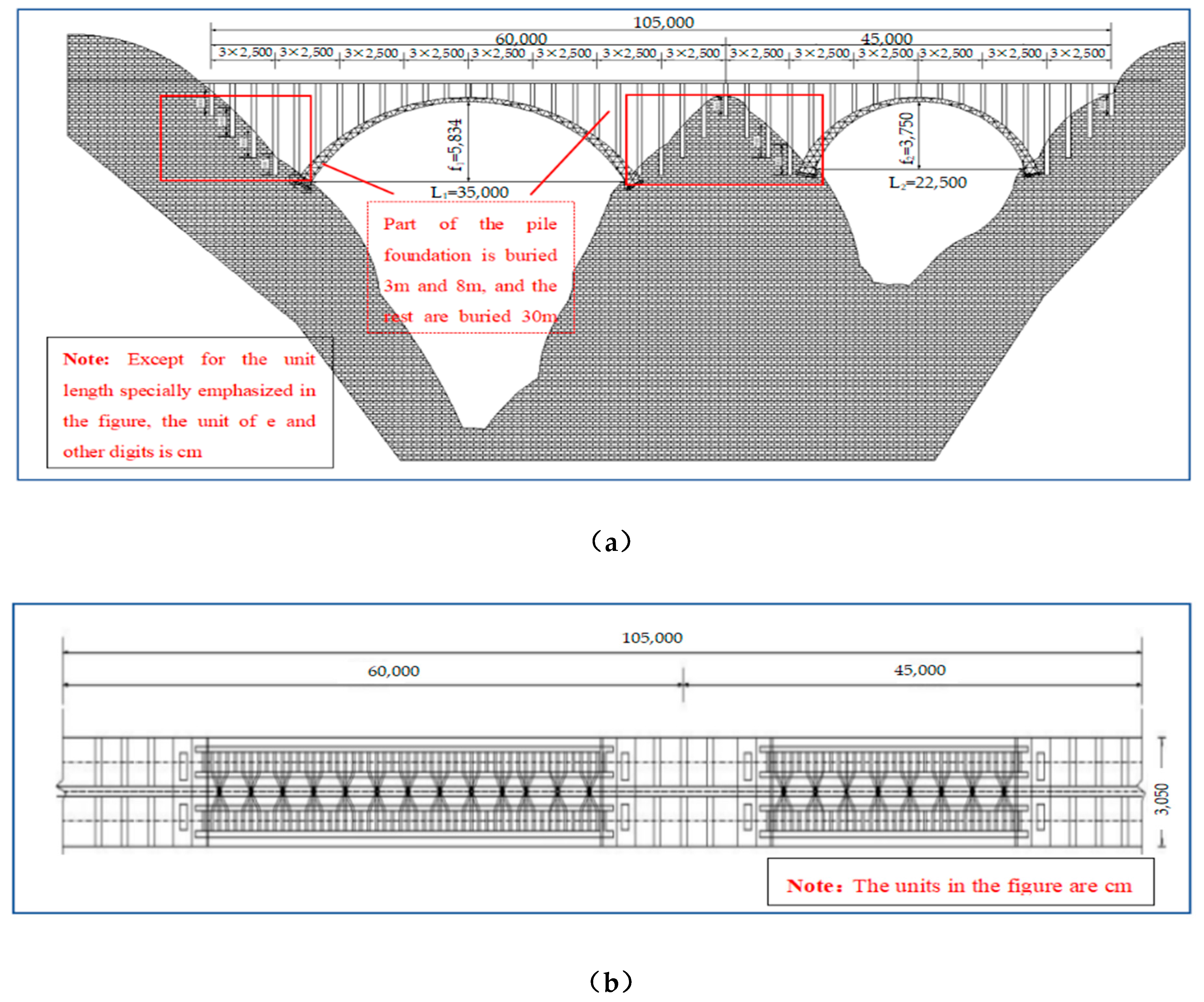
2. The Projects

Overview of Dependent Projects

The focus of this paper is a bridge located in the karst mountain and deep valley geomorphic area of Sichuan Province. The left bridge spans the No. 1 Deep Valley, with an upper arch span of 350 m, while the right bridge crosses Deep Valley Area No. 2, with an upper arch span of 225 m. The lower part of the bridge site features an asymmetrical “W”-shaped valley, with a cutting depth ranging from 270 to 450 m, and a river bed width of approximately 15 m. The elevation is around 420 m, and the banks consist of steep slopes and cliffs. The total length of the bridge is 1050 m.

The main bridge design consists of an overbearing concrete double-arch structure, with pile foundations buried at depths of 3 m and 8 m on the middle hillside for each span, respectively. The arch axis follows a quadratic parabola, with an arch axis coefficient m = 1.35. The main bridge deck utilizes pre-stressed concrete T-beams measuring about 22 m in length, while the structure consists of simply supported continuous bridge decks. Concrete solid piers are used for connecting piers. For the lower approach parts of the bridges, rectangular double pier pile foundations are employed, whereas pile-covered beam gravity abutments are utilized for the bridge abutments. Figure 1 illustrates the layout design featuring a “W”-type double-cut canyon concrete structure bridge.

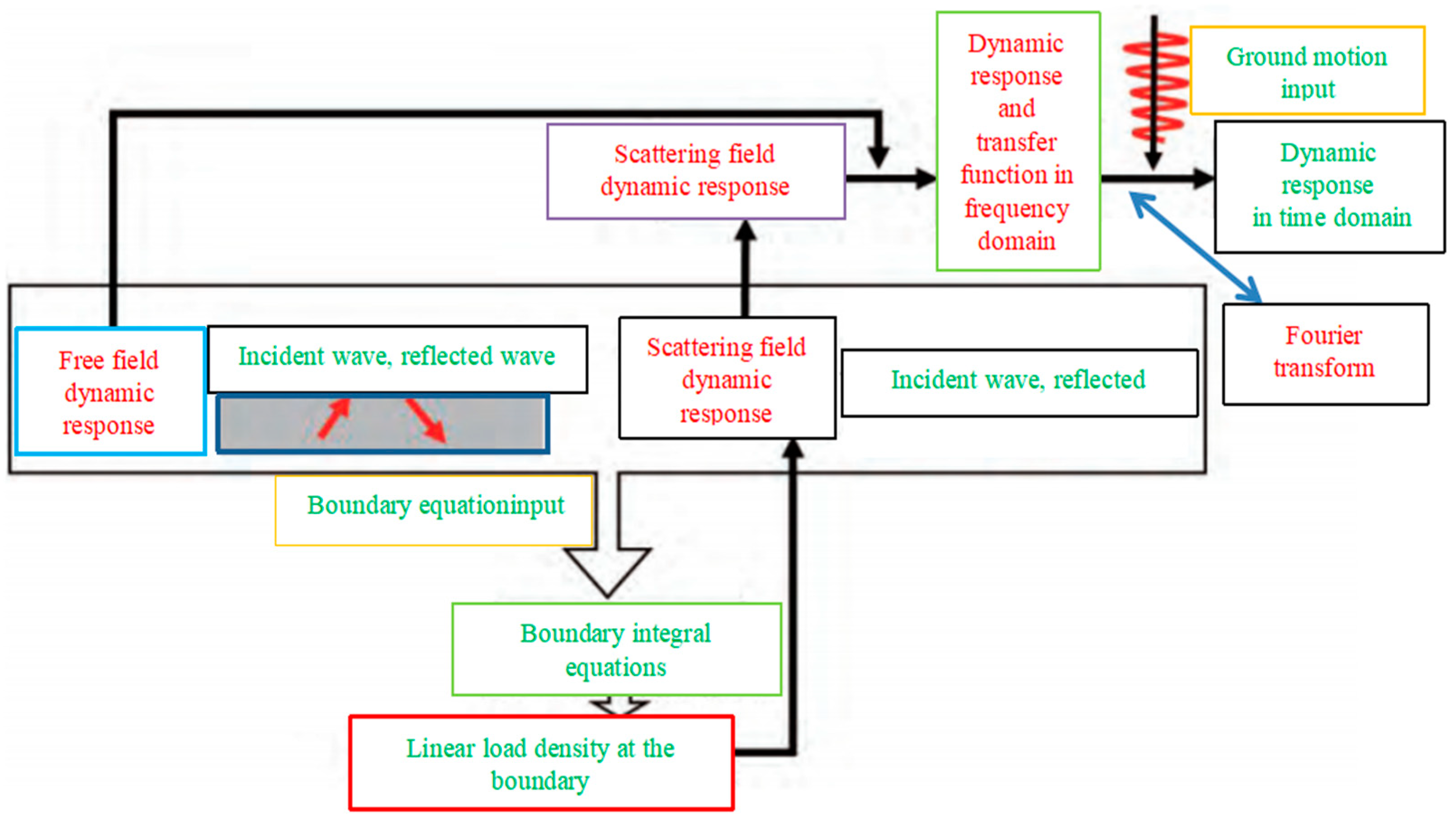
3. Formula Calculation Principle

3.1. Boundary Integral Equation Method

The boundary integral equation method was used to calculate the seismic wave propagation law in the deep valley under different load strengths, and the change in peak acceleration value at the slope foot of the arch bridge a₁, a₂, and a₃. The specific process of the method is: by analyzing the dynamic response of two free fields, the dynamic response and transfer function in the frequency domain are obtained, and then the dynamic response at different points in the region is determined by using the ground motion history and Fourier transform. The effect of the assumed mountain boundary conditions should be considered when dealing with the scattering field, and the virtual non-linear load density at the boundary can be converted by establishing the mountain and canyon boundary equations. The specific calculation process is shown in Figure 2.

Considering the complex influence of deep canyon topography on seismic wave propagation, the seismic response characteristics will enable mountain and arch bridge structures to withstand stronger earthquake forces. In this scenario, ground motion will significantly amplify the effect on the structure, resulting in a highly intricate process. To simplify the analysis, we can make the following assumptions in our model: that the soil layer medium is a viscoelastic isotropic material, and that the incident waves are harmonic P waves and SV waves. Under these assumptions, two types of wave fields exist in valley regions: the free field represents the original seismic wave field unaffected by terrain, while the scattered field is an additional wave field generated by wave reflection and refraction caused by terrain fluctuation. Therefore, within our model, each element is divided into blocks to calculate the dynamic response of arch bridges under the action of these two wave fields. The divided cell board is illustrated in Figure 3.

For the convenience of calculation, the W-shaped deep canyon terrain is divided into four blocks—${\mathrm{\Omega }}_1$ is the semi-space area (the part outside the area), and the regional part of the three mountains and the upper and lower boundaries of the region are shown in the Figure. Any time–history of ground motion is equivalent to the sum of a series of simple harmonics. Therefore, for a linear system, the dynamic response of the system under the excitation of simple harmonics should be studied first to obtain the transfer function in the frequency domain, and the dynamic response of the linear system under the incident time–history of arbitrary ground motion can be obtained by using inverse Fourier transform technology.

The meaning of parameters in Figure 3 indicates that the W-shaped deep canyon terrain is divided into four blocks for the convenience of calculation. ${\mathrm{\Omega }}_1$ is the half-space area (${\mathrm{\Omega }}_2$, ${\mathrm{\Omega }}_3$, ${\mathrm{\Omega }}_4$ the parts outside the area), ${\mathrm{\Omega }}_2$, ${\mathrm{\Omega }}_3$, ${\mathrm{\Omega }}_4$ are the regional parts of the three mountains, and ${\mathrm{\Gamma }}_n$ is the upper and lower boundaries of the divided area. Any time–history of ground motion can be equivalent to the sum of a series of simple harmonics. Therefore, in the case of a linear system, it is essential to first analyze the dynamic response of the system when subjected to simple harmonic excitation in order to determine its transfer function in the frequency domain. Subsequently, the dynamic response of the linear system under arbitrary ground motion can be obtained using inverse Fourier transform technology.

When the seismic wave is input at the bottom of the model, the wave function of the incident P wave reflecting the P wave and the SV wave is:

$${\mathrm{\Phi }}^{\mathrm{i}}{=\exp [-\mathrm{ik}}_{\mathrm{p}}(\mathrm{x}\sin {\theta }_{\mathrm{p}}-\mathrm{y}\cos {\theta }_{\mathrm{p}}{\left)\right]\mathrm{e}}^{\mathrm{iwt}}$$

(1)

$${\mathrm{\Phi }}^{\mathrm{r}}{=\mathrm{A}}_{\mathrm{pp}}{\exp [-\mathrm{ik}}_{\mathrm{p}}(\mathrm{x}\sin {\theta }_{\mathrm{p}}+\mathrm{y}\cos {\theta }_{\mathrm{p}}{\left)\right]\mathrm{e}}^{\mathrm{iwt}}$$

(2)

$${\mathrm{\Psi }}^{\mathrm{r}}{=\mathrm{A}}_{\mathrm{ps}}{\exp [-\mathrm{ik}}_{\mathrm{s}}(\mathrm{x}\sin {\theta }_{\mathrm{s}}+\mathrm{y}\cos {\theta }_{\mathrm{s}}{\left)\right]\mathrm{e}}^{\mathrm{iwt}}$$

(3)

$$A_{\mathrm{pp}}={\displaystyle \frac{\sin 2{\theta }_{\mathrm{p}}\sin 2{\theta }_{\mathrm{s}}{-\left[\right(\mathrm{k}}_{\mathrm{s}}{/\mathrm{k}}_{\mathrm{p}})\mathrm{gcos}2{\theta }_{\mathrm{s}}{]}^2}{\sin 2{\theta }_{\mathrm{p}}\sin 2{\theta }_{\mathrm{s}}{+\left[\right(\mathrm{k}}_{\mathrm{s}}{/\mathrm{k}}_{\mathrm{p}})\mathrm{gcos}2{\theta }_{\mathrm{s}}{]}^2}}$$

(4)

$$A_{\mathrm{ps}}={\displaystyle \frac{2\sin 2{\theta }_{\mathrm{p}}\cos 2{\theta }_{\mathrm{s}}}{\sin 2{\theta }_{\mathrm{p}}\sin 2{\theta }_{\mathrm{s}}+{[(k_{\mathrm{s}}/k_{\mathrm{p}})·\cos 2{\theta }_{\mathrm{s}}]}^2}}$$

(5)

where $e^{\mathrm{iwt}}$ is the time factor; $f$ is the incident frequency; $\omega$ is the circular frequency, where $\omega =2\pi f$; $k_{\mathrm{p}}$ and $k_{\mathrm{s}}$, respectively, are the waves of the P wave and the SV wave, $k_{\mathrm{p}}={\displaystyle \frac{\omega }{c_{\mathrm{p}}}}$, $k_{\mathrm{s}}={\displaystyle \frac{\omega }{c_{\mathrm{s}}}}$; ${\theta }_{\mathrm{p}}$ and ${\theta }_{\mathrm{s}}$ are the angles between the propagation direction and vertical direction of the P wave and the SV wave, respectively. $A_{\mathrm{pp}}$ and $A_{\mathrm{ps}}$ are the reflection coefficients of the P and SV waves, respectively.

The displacement, stress, and tractive force of the free field ${\mathsf{\Omega }}_1$ in half-space are, respectively:

$$u_{\mathrm{x}}^{\mathrm{f}}={\displaystyle \frac{\partial \mathrm{\Phi }}{\partial x}}+{\displaystyle \frac{\partial \mathrm{\Psi }}{\partial x}},u_{\mathrm{y}}^{\mathrm{f}}={\displaystyle \frac{\partial \mathrm{\Phi }}{\partial y}}+{\displaystyle \frac{\partial \mathrm{\Psi }}{\partial x}}$$

(6)

$${\sigma }_{\mathrm{xx}}^{\mathrm{f}}=(\lambda +2\mu ){\displaystyle \frac{\partial u_{\mathrm{x}}^{\mathrm{f}}}{\partial x}}+\lambda {\displaystyle \frac{\partial u_{\mathrm{y}}^{\mathrm{f}}}{\partial y}}$$

(7)

$${\sigma }_{\mathrm{yy}}^{\mathrm{f}}=(\lambda +2\mu ){\displaystyle \frac{\partial u_{\mathrm{y}}^{\mathrm{f}}}{\partial y}}+\lambda {\displaystyle \frac{\partial u_{\mathrm{x}}^{\mathrm{f}}}{\partial x}}$$

(8)

$$\begin{array}{l}{\tau }_{\mathrm{xy}}^{\mathrm{f}}=\mu ({\displaystyle \frac{\partial u_{\mathrm{x}}^{\mathrm{f}}}{\partial y}}+{\displaystyle \frac{\partial u_{\mathrm{y}}^{\mathrm{f}}}{\partial x}})\\ t_{\mathrm{x}}^{\mathrm{f}}={\sigma }_{\mathrm{xx}}^{\mathrm{f}}{n}_1+{\tau }_{\mathrm{xy}}^{\mathrm{f}}{n}_2\\ {\tau }_{\mathrm{y}}^{\mathrm{f}}={\sigma }_{\mathrm{yy}}^{\mathrm{f}}{n}_2+{\tau }_{\mathrm{xy}}^{\mathrm{f}}{n}_1\end{array}$$

(9)

where: Superscript $f$ represents free field; $\lambda$ and $\mu$ are complex Lamet constants, where $\lambda +2\mu =\rho c_{\mathrm{p}}^2$, $\mu =\rho c_{\mathrm{s}}^2$; $\rho$ is the medium density; $n_1$ and $n_2$ are the cosine of the Angle between the outer normal vector and the X, Y co-ordinates.

The scattering field of the semi-space region ${\mathrm{\Omega }}_1$ and the regional parts of the three mountains ${\mathrm{\Omega }}_2$, ${\mathrm{\Omega }}_3$, and ${\mathrm{\Omega }}_4$ are caused by the virtual line-load imposed on the boundaries of each region, so the scattering field displacement and tractive force in the model are:

$$u_{\mathrm{i}}^{(\mathrm{s},\mathsf{\Theta })}(\overrightarrow{x})={\displaystyle {\int }_{\mathrm{\Gamma }}}{G}_{\mathrm{ij}}(\overrightarrow{x},\overrightarrow{\zeta }){\mathrm{\Phi }}_{\mathsf{\Theta },\mathrm{j}}(\overrightarrow{\zeta })dS(\overrightarrow{\zeta })$$

(10)

$$t_{\mathrm{i}}^{(\mathrm{s},\mathsf{\Theta })}(\overrightarrow{x})={\displaystyle {\int }_{\mathrm{\Gamma }}}{T}_{\mathrm{ij}}(\overrightarrow{x},\overrightarrow{\zeta }){\mathrm{\Phi }}_{\mathsf{\Theta },\mathrm{j}}(\overrightarrow{\zeta })dS(\overrightarrow{\zeta })+{\displaystyle \frac{1}{2}}{\delta }_{\mathrm{ij}}{\mathrm{\Phi }}_{\mathsf{\Theta },\mathrm{j}}(\overrightarrow{x})$$

(11)

where: superscript S is the scattered wave; $\mathrm{\Theta }$ corresponds to ${\mathrm{\Omega }}_1$, ${\mathrm{\Omega }}_2$, ${\mathrm{\Omega }}_3$, and ${\mathrm{\Omega }}_4$; $\mathrm{\Gamma }$ is the boundary of each divided area; $i$ and $j$ are the corresponding x–direction and y–direction, and the value is ($i,j=1,2$). ${\mathrm{\Phi }}_{\mathsf{\Theta },\mathrm{j}}(\overrightarrow{\zeta })$ is the virtual linear load density in the direction $\mathrm{\Theta }$ imposed on the boundary point $\overrightarrow{\zeta }$ of $j$ region; ${\delta }_{\mathrm{ij}}$ is the Kronecker $\delta$ function; $G_{\mathrm{ij}}(\overrightarrow{x},\overrightarrow{\zeta })$ and $T_{\mathrm{ij}}(\overrightarrow{x},\overrightarrow{\zeta })$ are, respectively, Green’s formula for the dynamic force of the concentrated load in the whole space, and the unit concentration force applied at $\overrightarrow{\zeta }$ in the direction of $j$, causing the displacement and traction at $\overrightarrow{x}$ in the direction of $i$, where $G_{\mathrm{ij}}(\overrightarrow{x},\overrightarrow{\zeta })$ and $T_{\mathrm{ij}}(\overrightarrow{x},\overrightarrow{\zeta })$ are expressed as:

$$\begin{array}{l}{G}_{\mathrm{ij}}(\overrightarrow{x},\overrightarrow{\zeta })={\displaystyle \frac{1}{i8p}}[{\displaystyle \frac{{\delta }_{\mathrm{ij}}{H}_0^{\left(2\right)}(k_{\mathrm{p}}r)}{c_{\mathrm{p}}^2}}+{\displaystyle \frac{{\delta }_{\mathrm{ij}}{H}_0^{\left(2\right)}(k_{\mathrm{s}}r)}{c_{\mathrm{s}}^2}}-\\ {\displaystyle \frac{(2{\gamma }_{\mathrm{i}}{\gamma }_{\mathrm{i}}-{\delta }_{ij})H_2^{\left(2\right)}(k_{\mathrm{p}}r)}{c_{\mathrm{p}}^2}}+{\displaystyle \frac{(2{\gamma }_{\mathrm{i}}{\gamma }_{\mathrm{i}}-{\delta }_{\mathrm{ij}})H_2^{\left(2\right)}(k_{\mathrm{s}}r)}{c_{\mathrm{s}}^2}}]\end{array}$$

(12)

$$\begin{array}{l}{T}_{\mathrm{ij}}(\overrightarrow{x},\overrightarrow{\zeta })={\displaystyle \frac{i\mu }{2pr}}\left\{\left[{\displaystyle \frac{H_2^{\left(2\right)}(k_{\mathrm{p}}r)}{c_{\mathrm{p}}^2}}-{\displaystyle \frac{{(H_2)}^2(k_{\mathrm{s}}r)}{c_{\mathrm{s}}^2}}+{\displaystyle \frac{\lambda D(k_{\mathrm{p}}r)}{2\mu c_{\mathrm{p}}^2}}\right]{\gamma }_{\mathrm{j}}{n}_{\mathrm{j}}\right\}+\left[{\displaystyle \frac{{(H_2)}^2(k_{\mathrm{p}}r)}{c_{\mathrm{p}}^2}}-{\displaystyle \frac{H_2^{\left(2\right)}(k_{\mathrm{s}}r)}{c_{\mathrm{s}}^2}}+{\displaystyle \frac{D(k_{\mathrm{s}}r)}{2c_{\mathrm{s}}^2}}\right]\left({\gamma }_{\mathrm{j}}{n}_{\mathrm{j}}+{\gamma }_{\mathrm{k}}{n}_{\mathrm{k}}{\delta }_{\mathrm{ij}}\right)+\\ {\gamma }_{\mathrm{i}}{\gamma }_{\mathrm{j}}{\gamma }_{\mathrm{k}}{n}_{\mathrm{k}}\left(C-{\displaystyle \frac{4H_2^{\left(2\right)}(k_{\mathrm{p}}r)}{c_{\mathrm{p}}^2}}+{\displaystyle \frac{4H_2^{\left(2\right)}(k_{\mathrm{s}}r)}{c_{\mathrm{s}}^2}}\right)\end{array}$$

(13)

$$C={\displaystyle \frac{D(k_{\mathrm{p}}r)}{c_{\mathrm{p}}^2}}-{\displaystyle \frac{D(k_{\mathrm{s}}r)}{c_{\mathrm{s}}^2}}$$

(14)

$$D(p){=\mathrm{pH}}_1^{\left(2\right)}(p)$$

(15)

$${\gamma }_{\mathrm{i}}={\displaystyle \frac{(x_{\mathrm{i}}-{\zeta }_{\mathrm{i}})}{\sqrt{{(x_2-{\zeta }_1)}^2-{(x_2-{\zeta }_2)}^2}}}$$

(16)

where: $H_{\mathrm{m}}^{\left(\mathrm{n}\right)}(·)$ is a Hankel function of class n and order m.

Considering the different conditions of the boundaries of ${\mathrm{\Omega }}_1$, ${\mathrm{\Omega }}_2$, ${\mathrm{\Omega }}_3$, and ${\mathrm{\Omega }}_4$ regions in the model, the boundary of ${\mathrm{\Gamma }}_1$ region ${\mathrm{\Omega }}_1$ is at the infinite far end, so the boundary can be regarded as zero stress, and the boundary of ${\mathrm{\Omega }}_2$, ${\mathrm{\Omega }}_3$, and ${\mathrm{\Omega }}_4$ is in the medium-free space end, so ${\mathrm{\Gamma }}_5$, ${\mathrm{\Gamma }}_6$, and ${\mathrm{\Gamma }}_8$. The boundary is set at zero stress, and ${\mathrm{\Gamma }}_3$ and ${\mathrm{\Gamma }}_7$ are in a hollow state at the end of a deep canyon, with soilless media contact, so the boundary is also set at zero. The stress and displacement continuity conditions for other auxiliary boundaries are:

Zero stress boundary conditions at ${\mathrm{\Gamma }}_3$ and ${\mathrm{\Gamma }}_7$.

$$\begin{array}{l}{t}_{\mathrm{i}}^{\left({\mathrm{s},\mathsf{\Omega }}_1\right)}\left(\overrightarrow{x}\right)=-t_{\mathrm{i}}^{\mathrm{f}}(\overrightarrow{x}),\overrightarrow{x}\in {\mathrm{\Gamma }}_1,{\mathrm{\Gamma }}_3\\ t_{\mathrm{i}}^{\left({\mathrm{s},\mathsf{\Omega }}_1\right)}\left(\overrightarrow{x}\right)=-t_{\mathrm{i}}^{\mathrm{f}}(\overrightarrow{x}),\overrightarrow{x}\in {\mathrm{\Gamma }}_1,{\mathrm{\Gamma }}_7\end{array}$$

(17)

Zero stress boundary conditions at ${\mathrm{\Gamma }}_5$, ${\mathrm{\Gamma }}_6$ and ${\mathrm{\Gamma }}_8$.

$$t_{\mathrm{i}}^{\left({\mathrm{s},\mathsf{\Omega }}_2\right)}\left(\overrightarrow{x}\right)=0,\overrightarrow{x}\in {\mathrm{\Gamma }}_5$$

(18)

$$t_{\mathrm{i}}^{\left({\mathrm{s},\mathsf{\Omega }}_3\right)}\left(\overrightarrow{x}\right)=0,\overrightarrow{x}\in {\mathrm{\Gamma }}_6$$

(19)

$$t_{\mathrm{i}}^{\left({\mathrm{s},\mathsf{\Omega }}_3\right)}\left(\overrightarrow{x}\right)=0,\overrightarrow{x}\in {\mathrm{\Gamma }}_8$$

(20)

The fundamental conditions of stress and displacement continuity for the additional auxiliary boundaries, specifically denoted as (${\mathrm{\Gamma }}_2$, ${\mathrm{\Gamma }}_4$, and ${\mathrm{\Gamma }}_9$) are as follows:

$$\begin{array}{l}{u}_{\mathrm{i}}^{{(\mathrm{s},\mathsf{\Omega }}_1)}(\overrightarrow{x})+u_{\mathrm{i}}^{\mathrm{f}}(\overrightarrow{x})=u_{\mathrm{i}}^{{(\mathrm{s},\mathsf{\Omega }}_2)}(\overrightarrow{x}),\overrightarrow{x}\in {\mathrm{\Gamma }}_2\\ t_{\mathrm{i}}^{{(\mathrm{s},\mathsf{\Omega }}_1)}(\overrightarrow{x})+t_{\mathrm{i}}^{\mathrm{f}}(\overrightarrow{x})=-t_{\mathrm{i}}^{{(\mathrm{s},\mathsf{\Omega }}_2)}(\overrightarrow{x}),\overrightarrow{x}\in {\mathrm{\Gamma }}_2\end{array}$$

(21)

$$\begin{array}{l}{u}_{\mathrm{i}}^{{(\mathrm{s},\mathsf{\Omega }}_1)}(\overrightarrow{x})+u_{\mathrm{i}}^{\mathrm{f}}(\overrightarrow{x})=u_{\mathrm{i}}^{{(\mathrm{s},\mathsf{\Omega }}_3)}(\overrightarrow{x}),\overrightarrow{x}\in {\mathrm{\Gamma }}_4\\ t_{\mathrm{i}}^{{(\mathrm{s},\mathsf{\Omega }}_1)}(\overrightarrow{x})+t_{\mathrm{i}}^{\mathrm{f}}(\overrightarrow{x})=-t_{\mathrm{i}}^{{(\mathrm{s},\mathsf{\Omega }}_3)}(\overrightarrow{x}),\overrightarrow{x}\in {\mathrm{\Gamma }}_4\end{array}$$

(22)

$$\begin{array}{l}{u}_{\mathrm{i}}^{{(\mathrm{s},\mathsf{\Omega }}_1)}(\overrightarrow{x})+u_{\mathrm{i}}^{\mathrm{f}}(\overrightarrow{x})=u_{\mathrm{i}}^{{(\mathrm{s},\mathsf{\Omega }}_3)}(\overrightarrow{x}),\overrightarrow{x}\in {\mathrm{\Gamma }}_9\\ t_{\mathrm{i}}^{{(\mathrm{s},\mathsf{\Omega }}_1)}(\overrightarrow{x})+t_{\mathrm{i}}^{\mathrm{f}}(\overrightarrow{x})=-t_{\mathrm{i}}^{{(\mathrm{s},\mathsf{\Omega }}_3)}(\overrightarrow{x}),\overrightarrow{x}\in {\mathrm{\Gamma }}_9\end{array}$$

(23)

The calculated displacements of free field and scattering field, and the tractive force formula (Formulas (6)–(11)) are substituted into the boundary condition equation (Formulas (17)–(23)), and then all the boundaries (${\mathrm{\Gamma }}_1$–${\mathrm{\Gamma }}_9$) are discretized into $N_1$–$N_9$ units, and a set of linear square x–path groups are obtained through data conversion.

$$\begin{array}{l}{\displaystyle \sum _{\mathrm{l}}{\mathrm{\Phi }}_{{\mathsf{\Omega }}_1,\mathrm{j}}(\overrightarrow{{\zeta }_{\mathrm{l}}})}{t}_{\mathrm{ij}}(\overrightarrow{x_{\mathrm{n}}},\overrightarrow{{\zeta }_{\mathrm{l}}})=-t_{\mathrm{i}}^{\mathrm{f}}(\overrightarrow{x_{\mathrm{n}}}),\overrightarrow{x_{\mathrm{n}}}={\mathrm{\Gamma }}_1,{\mathrm{\Gamma }}_3\\ {\displaystyle \sum _{\mathrm{l}}{\mathrm{\Phi }}_{{\mathsf{\Omega }}_1,\mathrm{j}}(\overrightarrow{{\zeta }_{\mathrm{l}}})}{t}_{\mathrm{ij}}(\overrightarrow{x_n},\overrightarrow{{\zeta }_{\mathrm{l}}})=-t_{\mathrm{i}}^{\mathrm{f}}(\overrightarrow{x_{\mathrm{n}}}),\overrightarrow{x_{\mathrm{n}}}={\mathrm{\Gamma }}_1,{\mathrm{\Gamma }}_7\end{array}$$

(24)

$${\displaystyle \sum _{\mathrm{l}}{\mathrm{\Phi }}_{{\mathsf{\Omega }}_2,\mathrm{j}}(\overrightarrow{{\zeta }_{\mathrm{l}}})}{t}_{\mathrm{ij}}(\overrightarrow{x_{\mathrm{n}}},\overrightarrow{{\zeta }_{\mathrm{l}}})=0,\overrightarrow{x_{\mathrm{n}}}={\mathrm{\Gamma }}_5$$

(25)

$${\displaystyle \sum _{\mathrm{l}}{\mathrm{\Phi }}_{{\mathsf{\Omega }}_3,\mathrm{j}}(\overrightarrow{{\zeta }_{\mathrm{l}}})}{t}_{\mathrm{ij}}(\overrightarrow{x_{\mathrm{n}}},\overrightarrow{{\zeta }_{\mathrm{l}}})=0,\overrightarrow{x_{\mathrm{n}}}={\mathrm{\Gamma }}_6$$

(26)

$${\displaystyle \sum _{\mathrm{l}}{\mathrm{\Phi }}_{{\mathsf{\Omega }}_3,\mathrm{j}}(\overrightarrow{{\zeta }_{\mathrm{l}}})}{t}_{\mathrm{ij}}(\overrightarrow{x_{\mathrm{n}}},\overrightarrow{{\zeta }_{\mathrm{l}}})=0,\overrightarrow{x_{\mathrm{n}}}={\mathrm{\Gamma }}_8$$

(27)

The linear equations at different boundaries are obtained by the above formula.

$${\displaystyle \sum _{\mathrm{l}}{\mathrm{\Phi }}_{{\mathsf{\Omega }}_1,\mathrm{j}}(\overrightarrow{{\zeta }_{\mathrm{l}}})}{g}_{\mathrm{ij}}(\overrightarrow{x_{\mathrm{n}}},\overrightarrow{{\zeta }_{\mathrm{l}}})-{\displaystyle \sum _{\mathrm{l}}{\mathrm{\Phi }}_{{\mathsf{\Omega }}_{2,}\mathrm{j}}(\overrightarrow{{\zeta }_{\mathrm{l}}})}{g}_{\mathrm{ij}}(\overrightarrow{x_{\mathrm{n}}},\overrightarrow{{\zeta }_{\mathrm{l}}})=-u_{\mathrm{i}}^{\mathrm{f}}(\overrightarrow{x_{\mathrm{n}}}),\overrightarrow{x_{\mathrm{n}}}={\mathrm{\Gamma }}_2$$

(28)

$${\displaystyle \sum _{\mathrm{l}}{\mathrm{\Phi }}_{{\mathsf{\Omega }}_1,\mathrm{j}}(\overrightarrow{{\zeta }_{\mathrm{l}}})}{g}_{\mathrm{ij}}(\overrightarrow{x_{\mathrm{n}}},\overrightarrow{{\zeta }_{\mathrm{l}}})+{\displaystyle \sum _{\mathrm{l}}{\mathrm{\Phi }}_{{\mathsf{\Omega }}_{2,}\mathrm{j}}(\overrightarrow{{\zeta }_{\mathrm{l}}})}{g}_{\mathrm{ij}}(\overrightarrow{x_{\mathrm{n}}},\overrightarrow{{\zeta }_{\mathrm{l}}})=-t_{\mathrm{i}}^{\mathrm{f}}(\overrightarrow{x_{\mathrm{n}}}),\overrightarrow{x_{\mathrm{n}}}={\mathrm{\Gamma }}_2$$

(29)

$${\displaystyle \sum _{\mathrm{l}}{\mathrm{\Phi }}_{{\mathsf{\Omega }}_1,\mathrm{j}}(\overrightarrow{{\zeta }_{\mathrm{l}}})}{g}_{\mathrm{ij}}(\overrightarrow{x_{\mathrm{n}}},\overrightarrow{{\zeta }_{\mathrm{l}}})-{\displaystyle \sum _{\mathrm{l}}{\mathrm{\Phi }}_{{\mathsf{\Omega }}_{3,}\mathrm{j}}(\overrightarrow{{\zeta }_{\mathrm{l}}})}{g}_{\mathrm{ij}}(\overrightarrow{x_{\mathrm{n}}},\overrightarrow{{\zeta }_{\mathrm{l}}})=-u_{\mathrm{i}}^{\mathrm{f}}(\overrightarrow{x_{\mathrm{n}}}),\overrightarrow{x_{\mathrm{n}}}={\mathrm{\Gamma }}_4$$

(30)

$${\displaystyle \sum _{\mathrm{l}}{\mathrm{\Phi }}_{{\mathsf{\Omega }}_1,\mathrm{j}}(\overrightarrow{{\zeta }_{\mathrm{l}}})}{g}_{\mathrm{ij}}(\overrightarrow{x_{\mathrm{n}}},\overrightarrow{{\zeta }_{\mathrm{l}}})+{\displaystyle \sum _{\mathrm{l}}{\mathrm{\Phi }}_{{\mathsf{\Omega }}_{3,}\mathrm{j}}(\overrightarrow{{\zeta }_{\mathrm{l}}})}{g}_{\mathrm{ij}}(\overrightarrow{x_{\mathrm{n}}},\overrightarrow{{\zeta }_{\mathrm{l}}})=-t_{\mathrm{i}}^{\mathrm{f}}(\overrightarrow{x_{\mathrm{n}}}),\overrightarrow{x_{\mathrm{n}}}={\mathrm{\Gamma }}_4$$

(31)

$${\displaystyle \sum _{\mathrm{l}}{\mathrm{\Phi }}_{{\mathsf{\Omega }}_1,\mathrm{j}}(\overrightarrow{{\zeta }_{\mathrm{l}}})}{g}_{\mathrm{ij}}(\overrightarrow{x_{\mathrm{n}}},\overrightarrow{{\zeta }_{\mathrm{l}}})-{\displaystyle \sum _{\mathrm{l}}{\mathrm{\Phi }}_{{\mathsf{\Omega }}_{3,}\mathrm{j}}(\overrightarrow{{\zeta }_{\mathrm{l}}})}{g}_{\mathrm{ij}}(\overrightarrow{x_{\mathrm{n}}},\overrightarrow{{\zeta }_{\mathrm{l}}})=-u_{\mathrm{i}}^{\mathrm{f}}(\overrightarrow{x_{\mathrm{n}}}),\overrightarrow{x_{\mathrm{n}}}={\mathrm{\Gamma }}_9$$

(32)

$${\displaystyle \sum _{\mathrm{l}}{\mathrm{\Phi }}_{{\mathsf{\Omega }}_1,\mathrm{j}}(\overrightarrow{{\zeta }_{\mathrm{l}}})}{g}_{\mathrm{ij}}(\overrightarrow{x_{\mathrm{n}}},\overrightarrow{{\zeta }_{\mathrm{l}}})+{\displaystyle \sum _{\mathrm{l}}{\mathrm{\Phi }}_{{\mathsf{\Omega }}_{3,}\mathrm{j}}(\overrightarrow{{\zeta }_{\mathrm{l}}})}{g}_{\mathrm{ij}}(\overrightarrow{x_{\mathrm{n}}},\overrightarrow{{\zeta }_{\mathrm{l}}})=-t_{\mathrm{i}}^{\mathrm{f}}(\overrightarrow{x_{\mathrm{n}}}),\overrightarrow{x_n}={\mathrm{\Gamma }}_9$$

(33)

The $g_{\mathrm{ij}}(\overrightarrow{x_{\mathrm{n}}},\overrightarrow{{\zeta }_{\mathrm{l}}})$ and $t_{\mathrm{ij}}(\overrightarrow{x_{\mathrm{n}}},\overrightarrow{{\zeta }_{\mathrm{l}}})$ parameters in Equations (24)–(33) are calculated as follows:

$$g_{\mathrm{ij}}(\overrightarrow{x_{\mathrm{n}}},\overrightarrow{{\zeta }_{\mathrm{l}}})={\displaystyle {\int }_{\overrightarrow{{\zeta }_{\mathrm{l}}}-\frac{\mathsf{\Delta }S}{2}}^{\overrightarrow{{\zeta }_{\mathrm{l}}}+\frac{\mathsf{\Delta }S}{2}}}{G}_{\mathrm{ij}}(\overrightarrow{x_{\mathrm{n}}},\overrightarrow{\zeta })dS(\overrightarrow{\zeta })$$

(34)

$$t_{\mathrm{ij}}(\overrightarrow{x_{\mathrm{n}}},\overrightarrow{{\zeta }_{\mathrm{l}}})={\displaystyle \frac{1}{2}}{\zeta }_{\mathrm{ij}}{\zeta }_{\mathrm{nl}}+{\displaystyle {\int }_{\overrightarrow{{\zeta }_{\mathrm{l}}}-\frac{\mathsf{\Delta }S}{2}}^{\overrightarrow{{\zeta }_{\mathrm{l}}}+\frac{\mathsf{\Delta }S}{2}}}{T}_{\mathrm{ij}}(\overrightarrow{x_{\mathrm{n}}},\overrightarrow{\zeta })dS(\overrightarrow{\zeta })$$

(35)

where: $\mathsf{\Delta }S$ is the length value of the set model boundary unit.

The displacement and stress of the scattered field at any point in the model can be obtained by solving the linear Equations (24)–(33) to obtain the virtual uniform route load density, and then substituting the formula into Equations (10) and (11) to obtain the unit amplitude plane simple harmonic data. The regularized displacement amplitude function $H_{\mathrm{j}}(f)$ can be defined as:

$$H_{\mathrm{j}}\left(f\right)={\displaystyle \frac{u_{\mathrm{j}}^{\mathrm{t}}(f)}{u_0^{\mathrm{i}}(f)}}$$

(36)

where $u_{\mathrm{j}}^{\mathrm{t}}(f)$ is the total wave field displacement of any point in the model when the wave with frequency $f$ is incident; $u_0^{\mathrm{i}}(f)$ is the displacement of the incident field at the origin when a wave of frequency $f$ is incident. Considering that the frequency domain transfer function has been obtained in the model, the dynamic response data of the linear system in the model can be obtained by using the inverse Fourier transform technique.

3.2. Peak Frequency Shifting Method

The peak frequency shift method was used to analyze the spectrum of the conducted wave by selecting the peak acceleration of the propagation. The peak frequency shift method can monitor the frequency change of the transmitted signal in real time, and it is relatively insensitive to external interference, and has the characteristics of strong timeliness and accurate monitoring data. The main principle of the peak frequency shift method is as follows: after sampling the input ground motion signal at the specified point, a series of discrete signal samples are obtained. The next step involves performing the discrete Fourier transform (DFT) or fast Fourier transform (FFT) operation on these sample sets to convert the signal from the time domain to the frequency domain. This process results in obtaining the spectrum of the signal. The frequency in each spectrum is analyzed and processed to find the peak of the signal, that is, the frequency component with the largest amplitude, and the wavelength data. The resulting peak frequency is compared with the previous recorded peak frequency, and the difference is converted by difference, filtering, or curve fitting. If there is a large difference between the two peak frequencies, this indicates that the frequency of the signal has changed. It is necessary to iterate the above steps continuously to finally calculate the frequency change of the output signal in the propagation path, and perform data processing according to the formula to obtain the peak acceleration of the sample point.

Select n points in the ${\mathrm{\Omega }}_1$, ${\mathrm{\Omega }}_2$, ${\mathrm{\Omega }}_3$, and ${\mathrm{\Omega }}_4$ regions of the model, and substitute the soil layer density, shear modulus, and ground motion wavelength measured at n points into Equation (38) to calculate the peak frequency of the point. The calculated peak frequency and the measured duration of the corresponding point are put into Equation (37) to obtain the main frequency of ground motion at the point, and then the peak frequency and main frequency of the point are obtained. The soil layer density, shear modulus, and ground motion wavelength corresponding to n points are substituted into Equation (38) to calculate the peak frequency of the point. The calculated peak frequency and the measured duration of the corresponding point are put into Equation (37) to obtain the main frequency of ground motion at the point, and then the peak frequency and main frequency at different points are obtained.

$$f_m=\sqrt{{\displaystyle \frac{(t_{\mathrm{n}+1}{f}_{\mathrm{p}}^{\mathrm{n}}-t_{\mathrm{n}}{f}_{\mathrm{p}}^{\mathrm{n}+1})f_{\mathrm{p}}^{\mathrm{n}}{f}_{\mathrm{p}}^{\mathrm{n}+1}}{t_{\mathrm{n}+1}{f}_{\mathrm{p}}^{\mathrm{n}+1}-t_{\mathrm{n}}{f}_{\mathrm{p}}^{\mathrm{n}+1}}}}$$

(37)

$${{\displaystyle f}}_{\mathrm{p}}^n=\sqrt{{\displaystyle \frac{\lambda +2G}{{\lambda }^2\rho }}}$$

(38)

where $\rho$ is the density of soil layer at the measuring point (g/cm³); G is the shear modulus (MPa) of the medium; $f_m$ is the main frequency; $t_n$ is the propagation time to a place; $f_p^n$ is the peak frequency propagated to a certain time; $\lambda$ is the wavelength of ground motion. The corresponding wavelengths of 0.1 g, 0.2 g, and 0.3 g are 329 m, 768 m, and 1289 m, respectively.

Combined with the data obtained by the finite element numerical software FLAC3D V7.0, the amplitude and frequency of each calculation point in the ${\mathrm{\Omega }}_1$, ${\mathrm{\Omega }}_2$, ${\mathrm{\Omega }}_3$, and ${\mathrm{\Omega }}_4$ soil layers within the model range were calculated by using the peak frequency shift method, and the analytical formula of ground motion attenuation factor Q was obtained, as shown in Equation (44).

The initial spectrum of ground motion propagation in the medium in the ${\mathrm{\Omega }}_1$, ${\mathrm{\Omega }}_2$, ${\mathrm{\Omega }}_3$, and ${\mathrm{\Omega }}_4$ regions is:

$$f={{\displaystyle f}}_p^n$$

(39)

$$\beta \left(f\right)={\displaystyle \frac{2f^2}{f_{\mathrm{m}}^2\sqrt{\pi }}}exp\left(-{\displaystyle \frac{f^2}{f_{\mathrm{m}}^2}}\right)$$

(40)

When the ground motion propagates under the soil layer medium in ${\mathrm{\Omega }}_1$, ${\mathrm{\Omega }}_2$, ${\mathrm{\Omega }}_3$, and ${\mathrm{\Omega }}_4$ regions, the amplitude spectrum of the ground motion propagated to each measurement point is as follows:

$$\beta \left(f,t\right)=A\left(t\right)\beta \left(f\right)exp\left({\displaystyle \frac{-\pi f{t}_n}{Q}}\right)$$

(41)

$${\beta }_1\left(f,t_1\right)=A\left(t_1\right)\beta \left(f\right)exp\left({\displaystyle \frac{-\pi f{t}_1}{Q}}\right)$$

(42)

$${\beta }_2\left(f,t_2\right)=A\left(t_2\right)\beta \left(f\right)exp\left({\displaystyle \frac{-\pi f{t}_2}{Q}}\right)$$

(43)

By dividing Equations (42) and (43) by the spectral ratio method, the attenuation factor Q of ground motion at each depth point and its corresponding relationship can be obtained, where ${\beta }_1\left(f,t_1\right),{\beta }_2\left(f,t_2\right)$ is the seismic wave spectrum at $t_1$, $t_2$ time.

$$Q={\displaystyle \frac{\pi f\left(t_2-t_1\right)}{ln\left(\frac{A\left(t_1\right)}{A\left(t_2\right)}\right)-ln\int \frac{{\beta }_2\left(f,t_2\right)}{{\beta }_1\left(f,t_1\right)}}}$$

(44)

where: A(t) is the influence of other aspects unrelated to frequency; $\beta \left(f\right)$ is the initial loading seismic wave frequency; ${\beta }_n\left(f,t_2\right)$ is the seismic wave spectrum at a certain time; Q is the attenuation factor.

$$\begin{array}{l}{f}_{\mathrm{n}}={\displaystyle \frac{\partial \beta \left(f,t\right)}{\partial f}}=A\left(t\right){\displaystyle \frac{\partial \beta \left(f\right)}{\partial f}}exp\left({\displaystyle \frac{-\pi f_{\mathrm{t}}{t}_{\mathrm{n}}}{Q}}\right)\\ +{\displaystyle \frac{2f_{\mathrm{t}}^2}{f_{\mathrm{m}}^2\sqrt{\pi }}}exp\left(-{\displaystyle \frac{f_{\mathrm{t}}^2}{f_{\mathrm{m}}^2}}\right)\left(-{\displaystyle \frac{2f_t}{f_{\mathrm{m}}^2}}\right)\end{array}$$

(45)

where $t_n$ represents the time required for the propagation of a seismic wave to reach each specific measuring point, this parameter captures the duration it takes for the wave to traverse the medium and arrive at its designated location. On the other hand, $f_t$ signifies the frequency of the seismic wave at a particular instant in time, reflecting the rate of oscillation or vibration of the wave at that moment. Furthermore, $f_n$ denotes the seismic wave frequency that corresponds specifically to the measuring point in question. This frequency is a characteristic of the wave as it interacts with the environment at that specific location and may vary due to factors such as the composition of the medium, the distance traveled, and other geophysical conditions.

$$g=0.002f_{\mathrm{n}}^2\beta \left(f,t\right)$$

(46)

Referring to the relationship between amplitude frequency and acceleration in simple harmonic motion, the calculated frequency and peak frequency of each point, and the initial loading seismic wave spectrum $\beta \left(f\right)$, are brought into Equation (44), attenuation factors Q and $f_n$ are converted into Equation (45), and the measured amplitude of each point is substituted into Equation (46) to obtain the peak acceleration g value of each measuring point. The specific process of this method is shown in Figure 4 below.

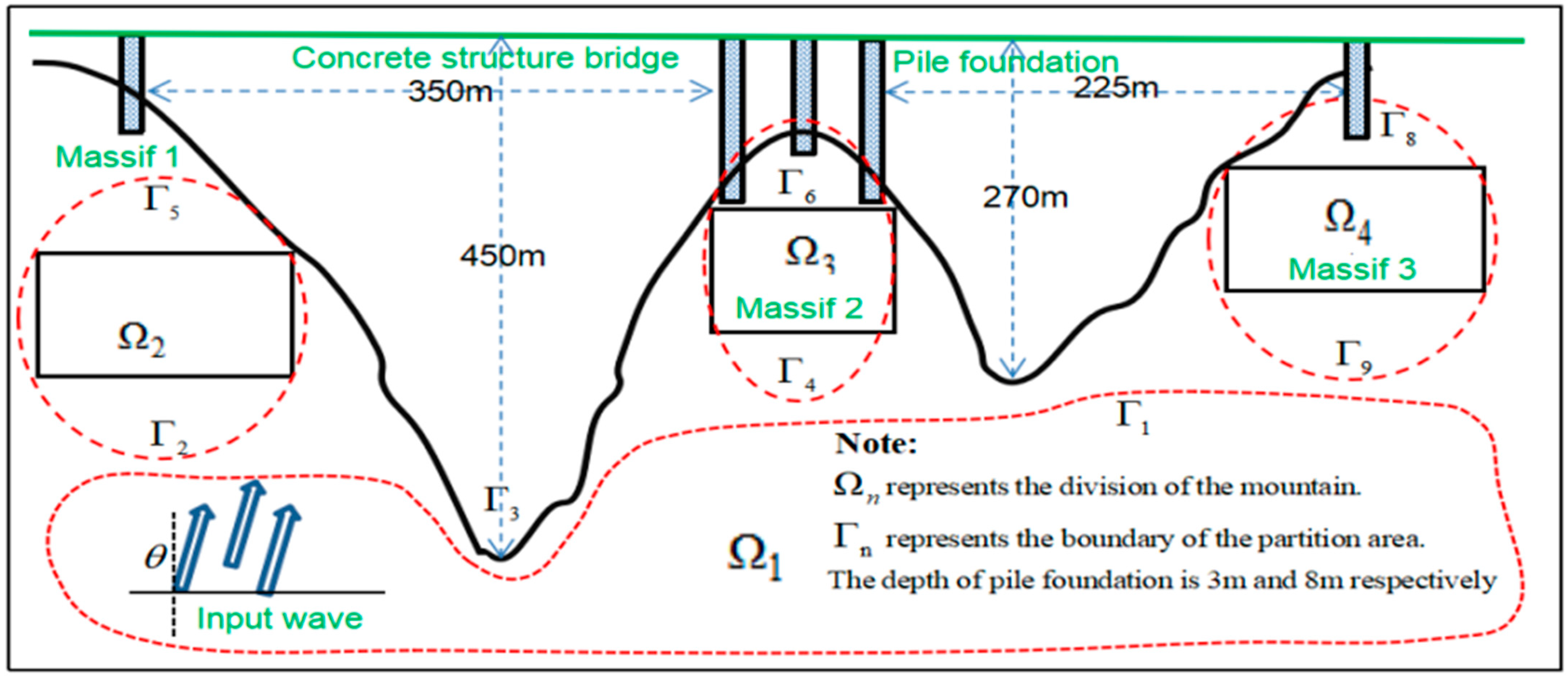
4. Model Construction

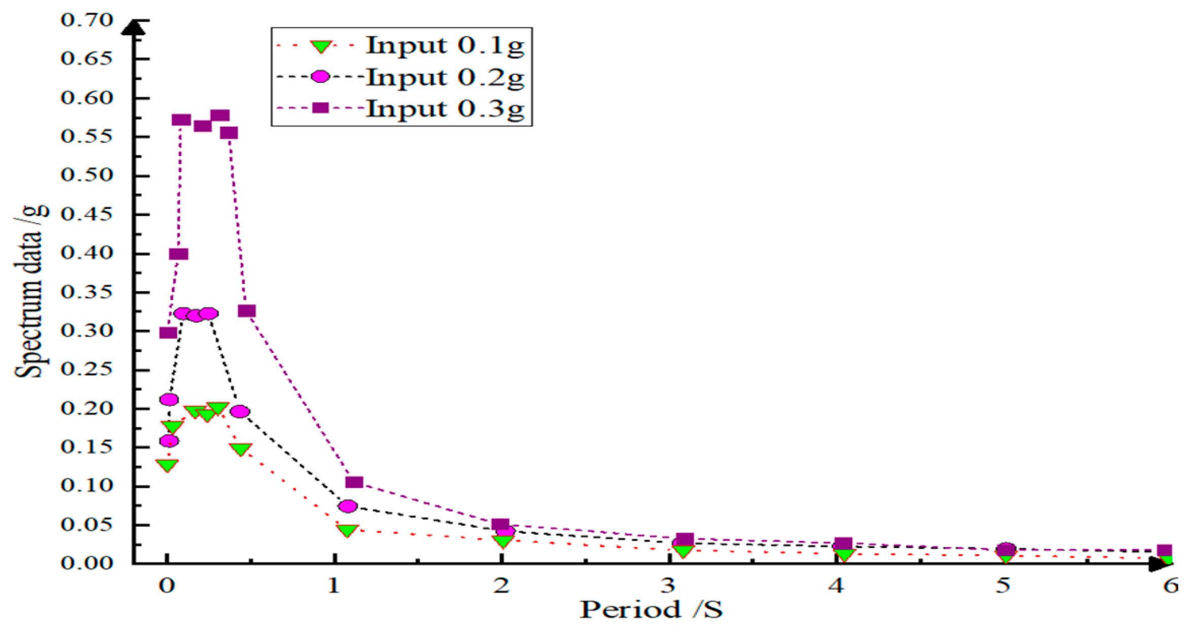
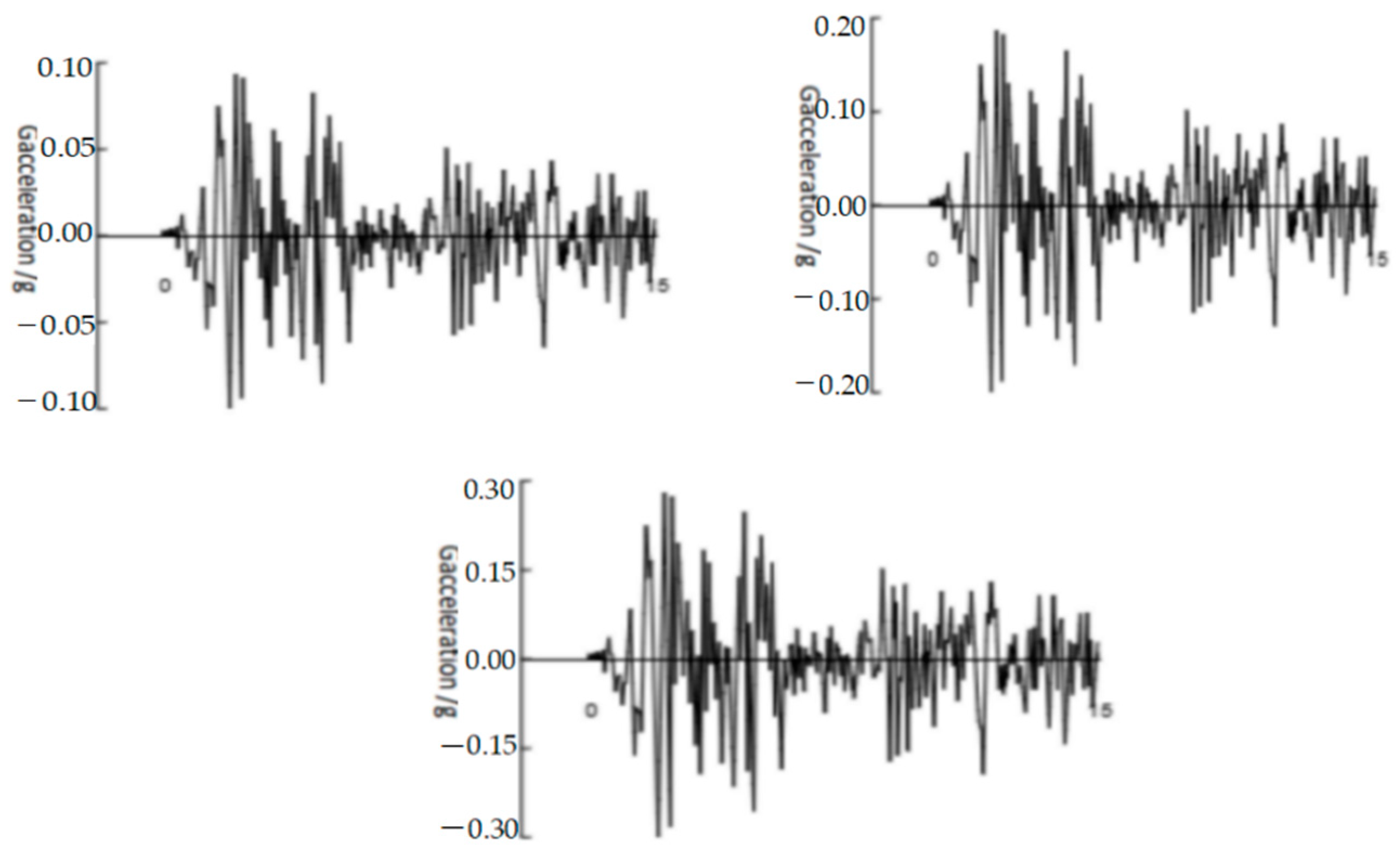
4.1. Loading Intensity and Corresponding Response Spectrum in the Model

Considering the frequent earthquakes in south-west China, the finite element spatial dynamic calculation model was loaded with ground motion data of 0.1 g, 0.2 g, and 0.3 g, respectively, to simulate the dynamic response characteristics of the overarching concrete structure bridge in the double-span “W” deep canyon terrain with seismic intensities of VII, VIII, and IX degrees, respectively. According to the spectrum data of the EI-Centro response spectrum in the Code for Seismic Design of Highway Bridges (JTG/T 2231-01-2020) [23], the ground motion duration of 0.1 g, 0.2 g, and 0.3 g artificial seismic waves was 15 s, and the time interval was 0.02 s. The fitted response spectrum is shown in Figure 5, and the artificial acceleration time wave is shown in Figure 6.

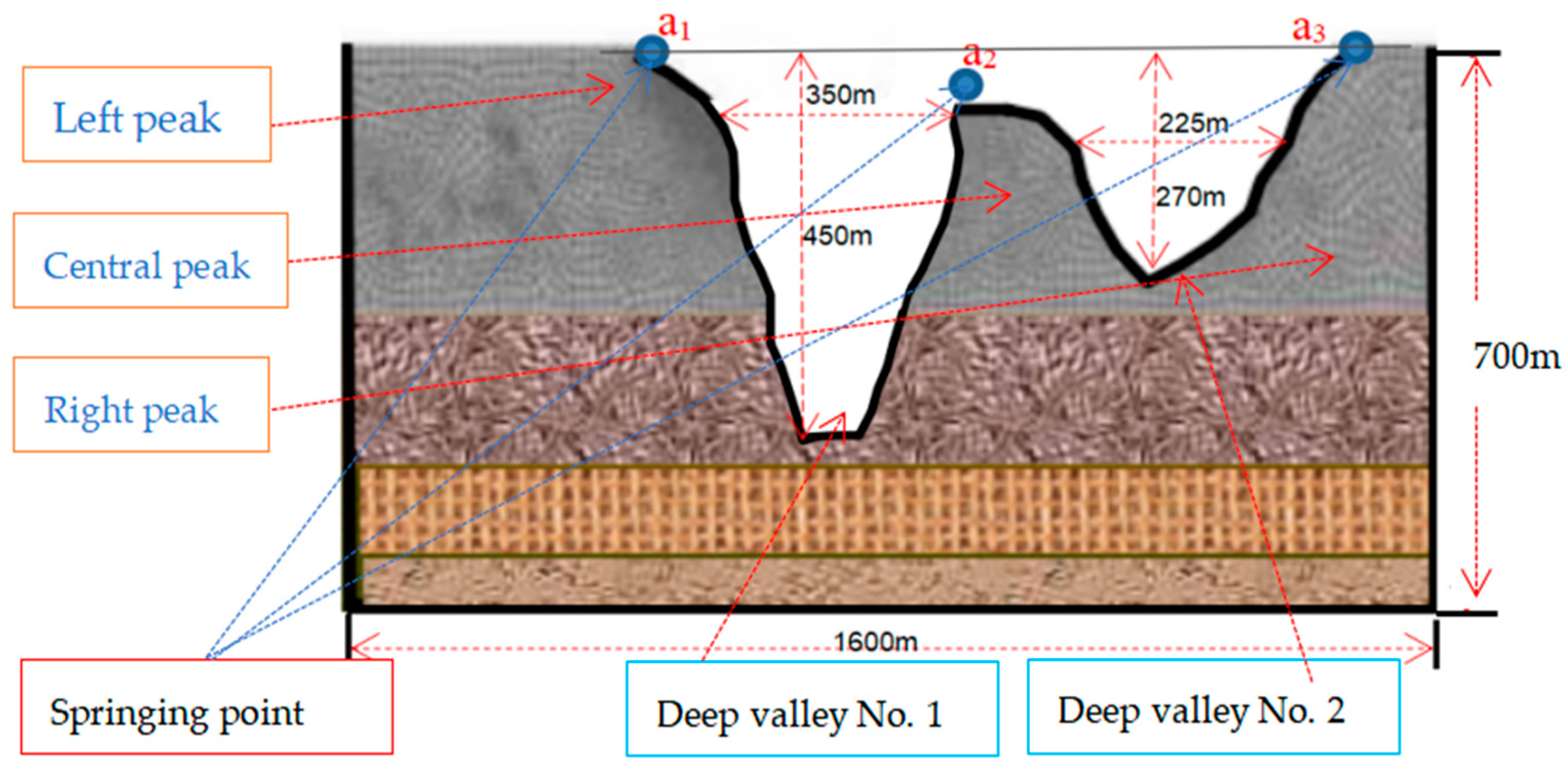
4.2. Establishment of Site Model

In order to simulate the effect of deep canyon topography on ground motion, it was necessary to establish a half-space plane strain model to simulate the façades of bridge sites. The span of the left main span of the bridge was 350 m, the span of the right main span was 225 m, the bottom of the left canyon to the top of the model is 450 m, and the right side is 150 m, the height of the model is 700 m, and the length of the model is 1600 m. Figure 6 shows the dimensioning comments of the W-shaped deep canyon site model. The artificial viscoelastic boundary was set to achieve the function of supporting the model to dissipate seismic energy, and a finite domain foundation was used to simulate an infinite domain foundation [24]. The viscoelastic boundary characteristics were determined by the spring stiffness and damping coefficient. The finite element model of deep canyon is shown in Figure 7.

5. Test Results

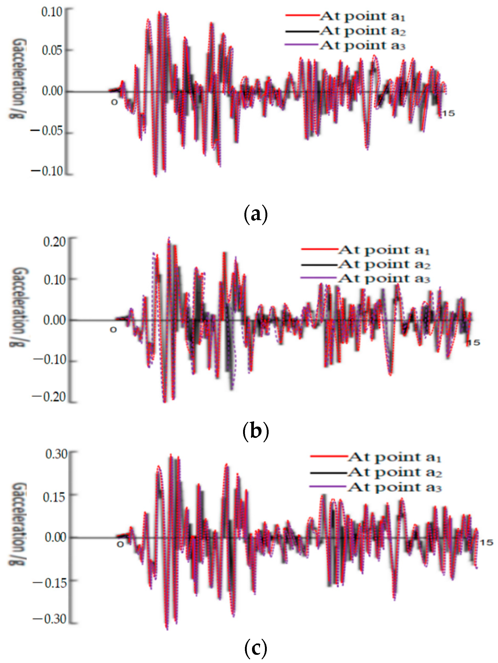
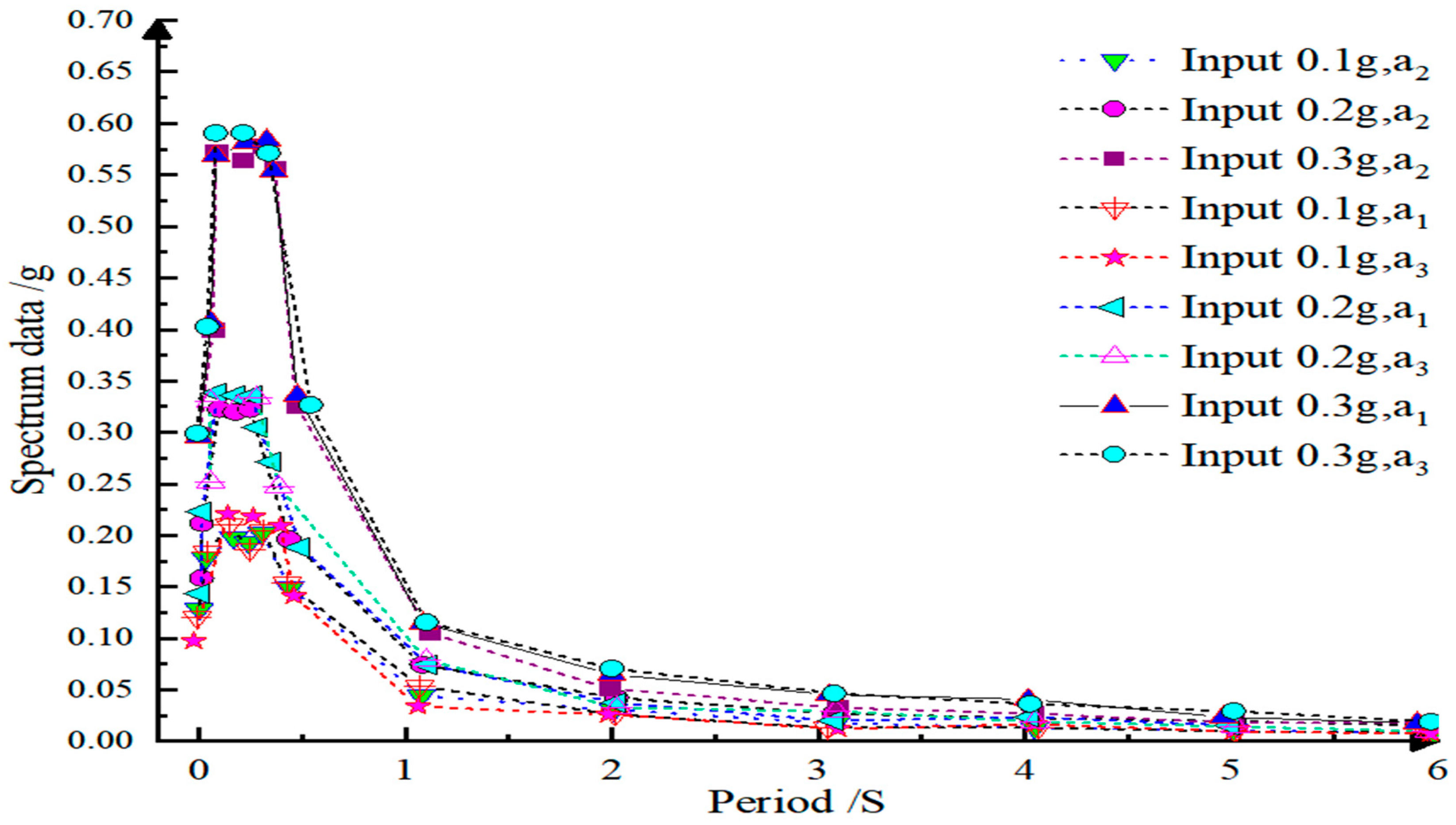
Analysis of Site Amplification Effect

EI-Centro waves of 0.1 g, 0.2 g, and 0.3 g were input into the finite element model to carry out the test, and then the acceleration time–history curve of the arch foot of the arch bridge at the measuring points a₁, a_2, and a₃ was recorded during the test, and its peak acceleration and spectral characteristics were analyzed, as shown in Figure 8 and Figure 9.

Under the input of 0.1 g, 0.2 g, and 0.3 g EI-Centro seismic waves, the peak acceleration data at the arch foot of a₁, a₂, and a₃, obtained by the finite element model, were compared with those obtained by the formula method. The corresponding amplification coefficient was obtained through data processing, as shown in

Table 1. Amplification coefficient of peak acceleration at each measuring point.

Station Position	Input Strength 0.1 g		Input Strength 0.2 g		Input Strength 0.3 g
	Peak Acceleration/g	Amplification Factor	Peak Acceleration/g	Amplification Factor	Peak Acceleration/g	Amplification Factor
a1	0.112	1.12	0.212	1.06	0.311	1.04
a2	0.103	1.03	0.201	1.01	0.304	1.01
a3	0.117	1.17	0.217	1.09	0.322	1.07
a1 (Formula method)	0.130	1.30	0.248	1.24	0.350	1.12
a2 (Formula method)	0.124	1.24	0.231	1.16	0.325	1.08
a3 (Formula method)	0.137	1.37	0.272	1.36	0.343	1.14

Note: amplification factor = measured value/input value.

.

By analyzing the data in Figure 8 and Figure 9, and Table 1, the seismic response of the arch bridge under the influence of EI-Centro seismic waves could be determined. The data indicate that the test values at the arch foot measured by the finite element method and those obtained by the formula method show a significant amplification of peak acceleration values at positions a₁, a₂, and a₃, exceeding the original ground motion input. This phenomenon suggests a notable field amplification effect at these key structural points.

It is worth noting that the amplification effect of the three arch foot positions is different, and the amplification effect is most significant at the arch foot of a₃. The arch foot of a₁ has a moderate amplification effect, while the arch foot of a₂ is closest to the input point and therefore shows the smallest amplification factor value. This difference in the magnification factor of different arch feet is mainly due to geological conditions.

At a₃, prominently protruding rock formations on the surface create a convergence effect for reflected seismic waves, intensifying the ground motion. In contrast, the rock mass at a1 presents a relatively flat surface profile, resulting in a diminished overlapping effect of reflected waves. The location of a₂, being closest to the input point, experiences the least modification of the original seismic waves. A thorough analysis of the response spectra presented in Figure 9 provides further insights into the impact of site effects on structural behavior. For short-period structures, the site effect significantly enhances their failure capacity under seismic loading. This suggests that the short-period elements of the bridge may exhibit greater resilience to earthquake damage than initially anticipated, based solely on the input ground motion. In contrast, for long-period structures, the site effect seems to have minimal influence on their seismic response. This indicates that the longer-period components of the bridge may respond to earthquakes in a manner more closely aligned with predictions based on the original ground motion data. In sections such as a₁, a₂, and a₃, the aforementioned approach is employed to enhance seismic performance. This includes reinforcing piers and foundations to increase overall stiffness, installing damping devices like dampers and isolation mounts to absorb and dissipate seismic energy, enhancing structural details and strengthening component connections, and reinforcing critical areas with new materials such as fiber-reinforced composites. Additionally, regular inspections and maintenance are conducted for timely detection and treatment of potential issues in order to enhance the bridge’s seismic capacity.

6. Influence of Site Effect on Structural Seismic Response

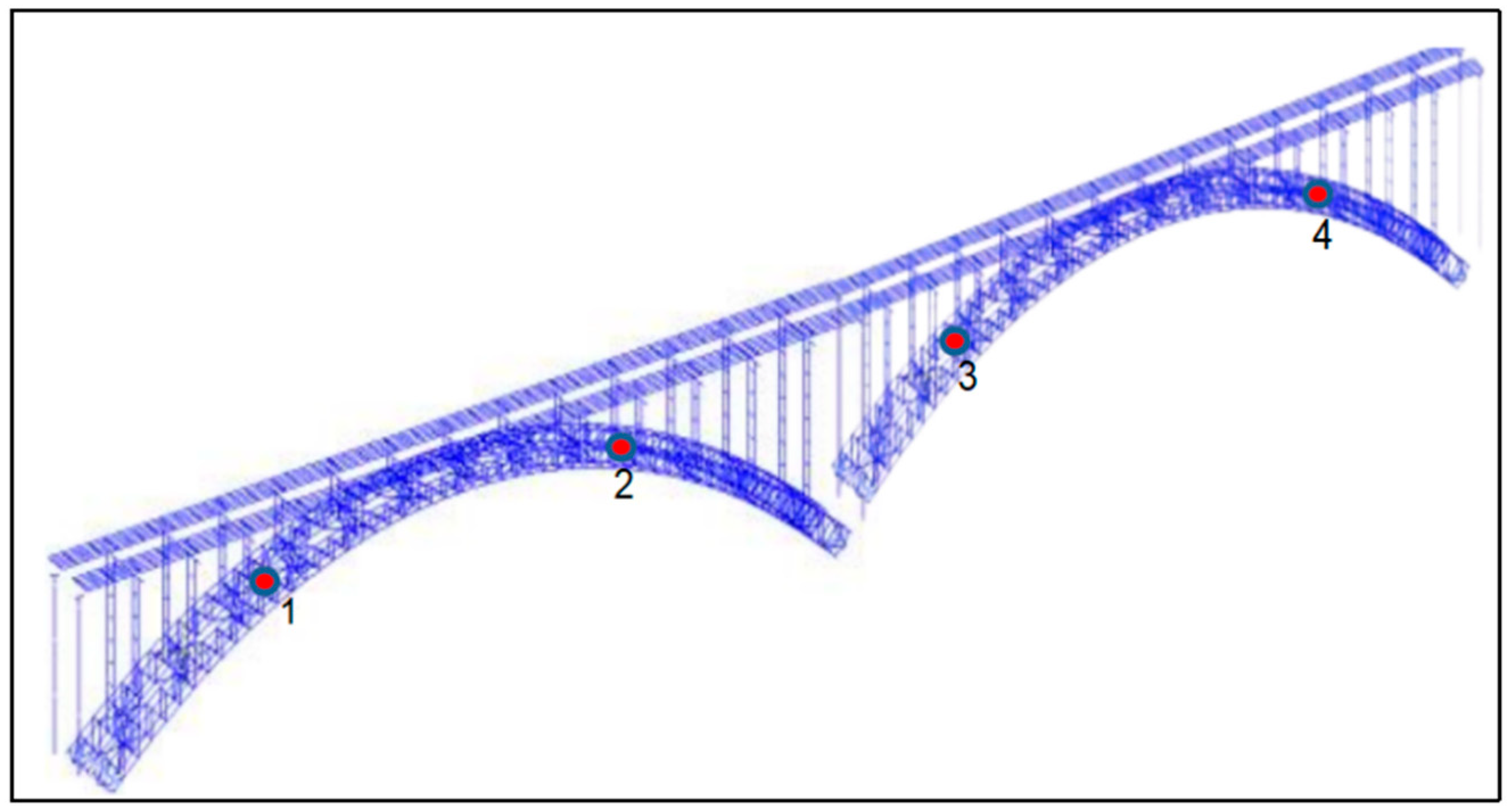
6.1. Dynamic Calculation Model

In order to analyze the seismic response of arch bridges to site effect, Midas Civil 2022 V 2.1 software was used to establish the comprehensive dynamic calculation model of arch bridge structure. This complex model employs multiple element types to accurately represent the different components of the bridge.

A detailed description of the complex geometry and stress distribution of arch foot steel plates is presented using plate elements. Beam elements are employed to effectively and accurately simulate most other structural components under seismic loads. The composite behavior and stress distribution of pre-stressed concrete T-beams can be carefully expressed through the use of the beam lattice method. Elastic connections are utilized to replicate the support conditions between the cap beam and the T-beam, simulating force transfer and deformation at these critical connections. To maintain simplicity and computational efficiency, certain factors such as approach bridges and pile-soil interactions have intentionally been omitted from the simulation, although they may potentially have significant effects. In order to enhance accuracy and reliability, special attention is given to areas with high stress concentration and complex load transfer when reinforcing two key locations within the finite element model.

The bottom pier is connected where significant forces are transferred between the superstructure and the substructure. The arch feet (three points) are subject to high stress concentration due to the unique geometry of the arch bridge. Figure 10 clearly illustrates these enhanced areas and provides a visual reference for the refinement of the model.

In order to consider the response of the site effect to the structure under vertical and longitudinal seismic action, this study focused on the calculation of the seismic response of the four upper ends of the arch bridge (measuring points 1–4). EI-Centro seismic waves were used as input ground motion to conduct time–history analysis of the bridge structure [25].

6.2. Analysis of Acceleration Response at the Top of the Structure under Different Loading Strengths

The top acceleration time–history curve can directly reflect the exciting effect of ground motion on the structure. In order to capture the effect of ground motion more accurately, the period from 0 to 15 s of ground motion was selected, and the acceleration response is the most intense in this range. The analysis results show that with the gradual increase in the intensity of the input seismic wave, the acceleration curve at the top of the arch bridge will fluctuate more violently, and the peak acceleration will also increase significantly, which is consistent with the mechanism of the impact response to the structure under the earthquake.

As shown in Figure 11, when the EI-Centro waves of 0.1 g, 0.2 g, and 0.3 g were input, respectively, the acceleration time–history curve at the top of the structural model with buried depths of 3 m and 8 m showed a fluctuating trend. Compared with Figure 11a,c,e, with the gradual increase of seismic wave intensity, the decrease in amplitude of acceleration at the top of the model with a depth of 3 m shows an increasing trend. Specifically, when the input intensity of the EI-Centro wave increases from 0.1 g to 0.3 g, the maximum acceleration at the top of the model increases from 0.38 g to 0.77 g, an increase of 102.63%. Similarly, by comparing Figure 11b,d,f, it was found that the acceleration response of the model with a depth of 8 m under the same seismic wave stimulation had the same trend as that of the model with a depth of 3 m. With the increase in seismic wave intensity at the input end, the decrease in amplitude of acceleration at the top of the model with a depth of 8 m also showed an increasing trend, and the increase in amplitude was obviously smaller than that of the model with a depth of 3 m. Specifically, when the intensity increased from 0.1 g to 0.3 g, the maximum acceleration at the top of the model with a depth of 8 m changed from 0.24 g to 0.43 g, with an increased ratio of 79.16%. These data demonstrate that increasing the buried depth under the same seismic action effectively reduces the acceleration response of the structure, thereby enhancing its seismic performance.

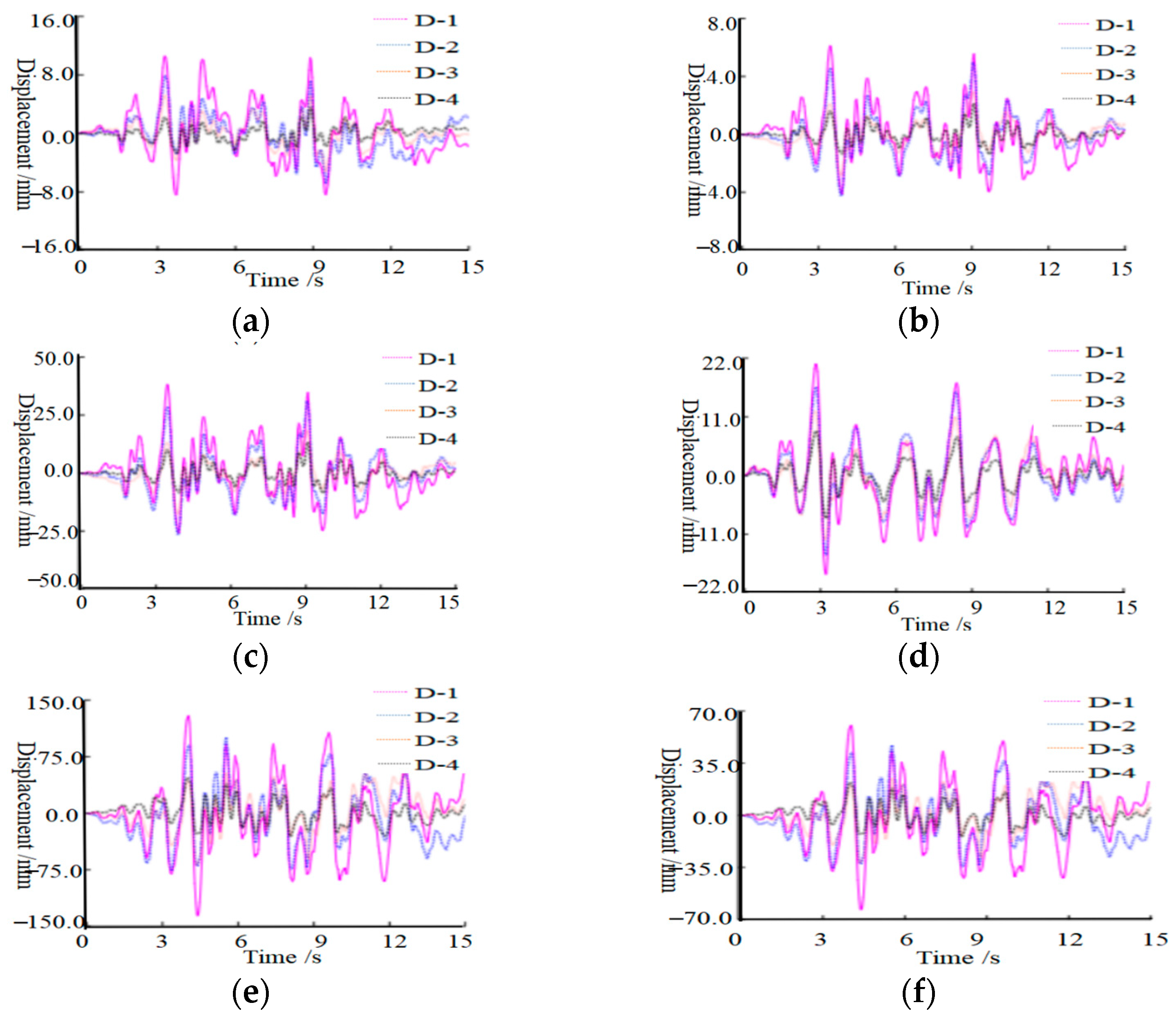
6.3. Displacement Analysis of the Top of the Structure under Different Loading Strengths

As shown in Figure 12, under the action of 0.1 g, 0.2 g, and 0.3 g EI-Centro waves, the top displacement time–history curves of the middle section of the arch bridge structure with the foundation buried depths of 3 m and 8 m, respectively, show different fluctuations. Although there are differences in seismic wave intensities, the top displacement time–history curves of the two arch bridge structural models with different buried depths show similar fluctuation trends under the same intensity of seismic wave excitation, which reflects the response characteristics of the structural models under earthquake action to a certain extent. It can be seen from the model diagram of a, c, and e buried depths of 3 m that the displacement at the top of the arch bridge structure increases with the gradual increase of seismic wave intensity. In particular, under the excitation of a 0.1 g seismic wave, the maximum displacement of the top is 8 mm; under the excitation of a 0.2 g seismic wave, the maximum displacement of the top is 32 mm. Under the excitation of a 0.3 g seismic wave, the maximum displacement of the top is 142 mm. According to the data in Figure 12b,d,f, it can be concluded that the maximum values of the corresponding top displacement under the input seismic wave intensities of 0.1 g, 0.2 g, and 0.3 g in the model are 6.2 mm, 21.1 mm, and 68.3 mm, respectively. The results show that the maximum displacement of the top of the 8-m buried depth model is smaller than that of the 3-m buried depth model under the same intensity of seismic wave excitation. This shows that the depth of stratum burial has a significant weakening effect on the propagation and scattering of seismic waves, that is, the acceleration peak propagated to the top of the structure is weakened. In conclusion, the analysis of the time–history curves of the top displacement of arch bridge structural models with buried depths of 3 m and 8 m under EI-Centro wave excitation reveals that the response of the two arch bridge foundations with different buried depths gradually increases under earthquake action as seismic wave intensity rises. However, due to variations in buried depth and other factors, there is a significant weakening effect on seismic wave propagation. Furthermore, it is observed that deeper buried depths result in better seismic performance for the arch bridge structure

7. Conclusions

This study focused on a bridge in Sichuan Province as the research subject. The study utilized the boundary integral equation method and the peak frequency shift method to develop an embedded linear time–history analysis algorithm for the full bridge finite element spatial dynamic calculation model, resulting in an enhanced model. The paper investigated the seismic response characteristics of the middle part of a W-shaped concrete arch bridge under different foundation depths and seismic intensities, comparing two methods with model test results. By comparing the test results of the finite element model with those obtained by combining the boundary integral equation method and peak frequency shift method formula, we can draw the following conclusions:

(1)

The site effect amplifies the peak value of acceleration and response spectrum, and changes the spectral characteristics of seismic waves. The amplification effect had a great influence on the seismic response of structures during a period of less than 2 s, but had no significant effect on the seismic response of structures during a period greater than 2 s. Moreover, the peak acceleration at the arch foot position of a₁, a₂, and a₃ was larger than the original seismic data, and the amplification effect at the arch foot position of a₃ was larger than that at the arch foot position of a₁ and a₂. The amplification effect was minimal at a₂ near the input point.

(2)

When the input seismic wave intensity increased from 0.1 g to 0.3 g, the maximum acceleration increase at the top of the 3-m model was 102.63%, while the acceleration increase of the 8-m model was 79.16%. This suggests that shallower buried structures are more sensitive to seismic wave strength.

(3)

Under the influence of 0.1 g, 0.2 g, and 0.3 g EI-Centro seismic waves, the maximum displacement at the top of the model with a foundation buried depth of 3 m was measured at 8 mm, 32 mm, and 142 mm, respectively. Similarly, for the model with a foundation depth of 8 m, the maximum displacements were recorded as 6.2 mm, 21 mm, and 68 mm for the corresponding seismic wave intensities. These findings suggest that an increase in foundation burial depth effectively reduces displacement at the structure’s apex due to enhanced constraint between deeply buried foundations and surrounding soil, leading to improved overall structural stiffness.

References

- Zhou, G.L.; Li, X.J.; Li, T.P.; Hou, C.L. Impact of canyon topography on seismic response of multi-supported long-span Bridges under SV wave incidence. Rock Soil Mech. 2012, 33, 1572–1578. [Google Scholar]
- Tan, Y.Q. Key Technology and Innovation of construction of steel pipe arch bridge connected by deep Canyon Bridge and tunnel. Railw. Constr. Technol. 2024, 5, 99–103. [Google Scholar]
- Zhang, X.X.; Zheng, S.X.; Tang, Y.; Zhang, L.Q.; Yuan, D.P. Numerical Simulation of Wind Parameters at long-span arch bridge site in Mountain Gorge. J. Railw. Sci. Eng. 2018, 15, 398–406. [Google Scholar]
- Wu, H.G.; Liang, Y.; Lai, T.W. Study on interaction mechanism between bridge and landslide under earthquake. J. Railw. Eng. 2023, 40, 54–61. [Google Scholar]
- Jia, Y.; Wang, Z.H.; Tian, H.; Liu, P.Z.; Song, H.B. Seismic response analysis of single-span asymmetric suspension bridge considering beam end impact. J. Shenyang Jianzhu Univ. (Nat. Sci. Ed.) 2023, 39, 1075–1083. [Google Scholar]
- Liao, Y.C.; Zhang, R.Y.; Lin, R.; Zong, Z.H.; Wu, G. Nonlinear seismic response prediction of Bridges based on cascading residual LSTM networks. Eng. Mech. 2024, 41, 47–58. [Google Scholar]
- Xu, L.Q.; Yuan, M.J.; Zuo, Y.; Shen, Z.X.; Xu, M.H. Nearly pulse type faults under the action of earthquake dynamic response analysis of long-span arch bridge. J. Vib. Shock 2024, 9, 94–104+148. [Google Scholar]
- Feng, J. Seismic response analysis of concrete-filled steel tube arch bridge in deep canyon. Highw. Traffic Technol. 2024, 1–11. [Google Scholar]
- Feng, Z.J.; Li, Y.T.; Zhao, R.X.; Cai, J.; Dong, J.S.; Meng, Y.Y. Research on dynamic response of pile group foundation with variable section in liquefiable site. Sci. Technol. Eng. 2023, 23, 7886–7894. [Google Scholar]
- Wang, J.H. Research on Seismic Response of Concrete-Filled Steel Tube Arch Bridge in Deep Canyon. Master’s Thesis, Chongqing Jiaotong University, Chongqing, China, 2023. [Google Scholar]
- Shi, C.Z.; Cheng, C.; Wang, Z.M.; Wu, H.G.; Hu, Y. Inverted siphon pipe bridge of large span structure seismic performance. J. Yangtze River Sci. Res. Inst. 2022, 33, 111–116. [Google Scholar]
- Chen, J.W.; Zheng, K.F.; Zuo, Z.C. Research on seismic response and damper parameter optimization of large-span railway steel truss flexible arch bridge. Sichuan Archit. 2023, 43, 94–104, 165. [Google Scholar]
- Li, X.Z.; Liu, M.; Yang, D.H.; Dai, S.Y.; Xiao, L. Earthquake damage evolution simulation of long-span top-bearing steel truss arch bridge. J. Southwest Jiaotong Univ. 2019, 55, 94–104, 1223. [Google Scholar]
- Shi, C.; Lin, P.Z.; Zhou, P.; He, Z.G. Spatial seismic response analysis of long-span continuous steel truss flexible arch bridge under multi-point excitation. J. Earthq. Eng. 2018, 40, 273–278. [Google Scholar]
- Xia, Z.H.; Zhang, X.Y.; Zong, Z.H. Analysis of Dynamic characteristics of reinforced concrete simply supported oblique wide beam bridge. J. Fuzhou Univ. (Nat. Sci. Ed.) 2008, 36, 278–283. [Google Scholar]
- Chen, B.; Zhao, L.; Chen, S.X.; Yue, Q. Analysis on dynamic characteristics of the second-line Niujiaoping Bridge added to Xiangyu Railway. Railw. Constr. 2007, 3, 1–4. [Google Scholar] [CrossRef]
- Huang, W.J.; Peng, G.H.; Chen, B.C.; Chen, Y.Y.; He, X.H.; Sun, C. Stress analysis of concrete-filled steel tube rigid frame tied arch bridge. J. Fuzhou Univ. (Nat. Sci. Ed.) 2004, 32, 190–194. [Google Scholar]
- Yun, D.; Liu, H.; Zhang, S.M. Half through bridge concrete filled steel tubular arch bridge seismic elastic-plastic time history analysis. J. Jilin Univ. (Eng. Sci.) 2014, 44, 1633–1638. [Google Scholar]
- Ye, D.; Zhou, J.T.; Wang, L.; Zhang, R.; Xu, L.; Jin, S. Seismic response analysis of long-span CFST arch bridge considering valley site effect. World Earthq. Eng. 2022, 38, 108–116. [Google Scholar]
- Luo, Y.H.; Wang, Y.S. Terrain amplification effect of mountain slope vibration induced by Wenchuan earthquake. J. Mt. Sci. 2013, 31, 200–210. [Google Scholar]
- Zhang, J.; Liang, J.W.; Ba, Z.N. When SH wave incident raised the site topography and soil amplification effect. Earthq. Eng. Eng. Vib. 2016, 4, 56–67. [Google Scholar]
- Fu, L.; Xie, J.J.; Chen, S.; Zhang, B.; Zhang, X.; Li, X.J. Characteristic analysis of site magnification factor and its application in simulation of strong ground motion in Sichuan area: A case study of the 2022 Lushan Ms6.1 earthquake. Geophys. J. 2023, 66, 2933–2950. [Google Scholar]
- JTG/T 2231-01-2020; Ministry of Transport of the People’s Republic of China. Code for Seismic Design of Highway Bridges. People’s Communications Press: Beijing, China, 2020.
- Luo, C.; Sheng, C.; Wan, J.Z.; Xu, C.R.; Guo, H.Q.; Wang, H. Influence of Rayleigh waves on seismic response of V-shaped valley arch bridge. Chin. J. Highw. Sci. 2023, 11, 1–17. [Google Scholar]
- Li, X.L.; Zou, Y.H.; Wang, D.S. Earthquake damage characteristics and aseismic research of bridge with arch system under strong earthquake. World Earthq. Eng. 2018, 34, 33–43. [Google Scholar]