Convergence Analysis for an Online Data-Driven Feedback Control Algorithm

Abstract

This paper presents convergence analysis of a novel data-driven feedback control algorithm designed for generating online controls based on partial noisy observational data. The algorithm comprises a particle filter-enabled state estimation component, estimating the controlled system’s state via indirect observations, alongside an efficient stochastic maximum principle-type optimal control solver. By integrating weak convergence techniques for the particle filter with convergence analysis for the stochastic maximum principle control solver, we derive a weak convergence result for the optimization procedure in search of optimal data-driven feedback control. Numerical experiments are performed to validate the theoretical findings.

1. Introduction

In this paper, we carry out numerical analysis demonstrating the convergence of a data-driven feedback control algorithm designed for generating online control based on partial noisy observational data.

Our focus lies on the stochastic feedback control problem, which aims to determine optimal controls. These control actions are used to guide a controlled state dynamical system towards meeting certain optimality conditions, leveraging feedback from the system’s current state. There are two practical challenges in solving the feedback control problem. First, when the control problem’s dimension is high, the computational cost for searching the optimal control escalates exponentially. This is known as the “curse of dimensionality”. Second, in numerous scenarios, the state of the controlled system is not directly observable and must be inferred through detectors or observation facilities. These sensors are typically subject to noise that originates from the device itself or the surrounding environment. For instance, radar receives noisy data and processes them through the arctangent function. Therefore, state estimation techniques become necessary to estimate the current state for designing optimal control, with observations gathered to aid in estimating the hidden state.

To address the aforementioned challenges, a novel online data-driven feedback control algorithm has been developed [1]. This algorithm introduces a stochastic gradient descent optimal control solver within the stochastic maximum principle framework to combat the high dimensionality issue in optimal control problems. Traditionally, stochastic optimal control problems are solved using dynamical programming or the stochastic maximum principle, both requiring numerical simulations for large differential systems [2,3,4]. However, the stochastic maximum principle stands out for its capability to handle random coefficients in the state model and finite-dimensional terminal state constraints [5]. In the stochastic maximum principle approach, a system of backward stochastic differential equations (BSDEs) is derived as the adjoint equation of the controlled state process. Then, the solution of the adjoint BSDE is utilized to formulate the gradient of the cost function with respect to the control process [6,7]. However, solving BSDEs numerically entails significant computational costs, especially in high-dimensional problems, demanding a large number of random samples [8,9]. To bolster efficiency, a sample-wise optimal control solver method has been devised [10], where the solution of the adjoint BSDE is represented using only one realization or a small batch of samples. This approach justifies the application of stochastic approximation in the optimization procedure [11,12], and it shifts the computational cost from solving BSDEs to searching for the optimal control, thereby enhancing overall efficiency [13].

In data-driven feedback control, optimal filtering methods also play a pivotal role in dynamically estimating the state of the controlled system. Two prominent approaches for nonlinear optimal filtering are the Zakai filter and the particle filter. While the Zakai filter aims to compute the conditional probability density function (pdf) for the target dynamical system using a parabolic-type stochastic partial differential equation known as the Zakai equation [14], the particle filter, also known as a sequential Monte Carlo method, approximates the desired conditional pdf using the empirical distribution of a set of random samples (particles) [15]. Although the Zakai filter theoretically offers more accurate approximations for conditional distributions, the particle filter is favored in more practical applications due to the high efficiency of the Monte Carlo method in approximating high-dimensional distributions [16].

The aim of this study is to examine the convergence of the data-driven feedback control algorithm proposed in [1], providing mathematical validation for its performance. While convergence in particle filter methods has been well studied [17,18,19], this work adopts the analysis technique outlined in [18] to establish weak convergence results for the particle filter regarding the number of particles. Analysis techniques for BSDEs alongside classical convergence results for stochastic gradient descent [13,20] are crucial for achieving convergence in the stochastic gradient descent optimal control solver. The theoretical framework of this analysis merges the examination of particle filters with the analysis of optimal control, and the overarching objective of this paper is to derive a comprehensive weak convergence result for the optimal data-driven feedback control.

In this paper, we present two numerical examples to demonstrate the baseline performance and convergence trend of our algorithm. The first example involves a classic linear quadratic optimal control problem, comparing the analytical control with the estimated control. The second example addresses a nonlinear scenario, specifically a Dubins vehicle maneuvering problem, where both the system and observations exhibit significant nonlinearity.

The rest of this paper is organized as follows. In Section 2, we introduce the data-driven feedback control algorithm. Convergence analysis will be presented in Section 3, and in Section 4, we conduct two numerical experiments to validate our theoretical findings.

2. An Efficient Algorithm for Data-Driven Feedback Control

We first briefly introduce the data-driven feedback control problem that we consider in this work. Then, we describe our efficient algorithm for solving the data-driven feedback control problem by using a stochastic gradient descent-type optimization procedure for the optimal control.

2.1. Problem Setting for the Data-Driven Optimal Control Problem

In probability space $(\mathrm{\Omega },\mathcal{F},\mathbb{P})$, we consider the following augmented system on time interval $[0,T]$

$$\begin{array}{c}\hfill d\left(\begin{array}{c}{X}_t\\ M_t\end{array}\right)=\left(\begin{array}{c}b(t,X_t,u_t)\\ g\left(X_t\right)\end{array}\right)dt+\left(\begin{array}{cc}\sigma (t,X_t,u_t)& 0\\ 0& I\end{array}\right)d\left(\begin{array}{c}{W}_t\\ B_t\end{array}\right),\left(\begin{array}{c}{X}_0=\xi \\ M_0=0\end{array}\right),\end{array}$$

(1)

where $X:={\left\{X_t\right\}}_{t=0}^T$ is the ${\mathbb{R}}^d$-dimensional controlled state process with dynamics $b:[0,T]\times {\mathbb{R}}^d\times {\mathbb{R}}^m\to {\mathbb{R}}^d$, $\sigma :[0,T]\times {\mathbb{R}}^d\times {\mathbb{R}}^m\to {\mathbb{R}}^{d\times q}$ is the diffusion coefficient for a d-dimensional Brownian motion W that perturbs the the state X, and u is an m-dimensional control process valued in some set U that controls the state process X. In the case that the state X is not directly observable, we have an observation process M that collects partial noisy observations on X with observation function $g:{\mathbb{R}}^d\to {\mathbb{R}}^p$, and B is a p-dimensional Brownian motion that is independent from W.

Let ${\mathbb{F}}^B={\left\{{\mathcal{F}}_t^B\right\}}_{t\ge 0}$ be the filtration of B augmented by all the $\mathbb{P}$-null sets in $\mathcal{F}$, and ${\mathbb{F}}^{W,B}\equiv {\left\{{\mathcal{F}}_t^{W,B}\right\}}_{t\ge 0}$ be the filtration generated by W and B (augmented by $\mathbb{P}$-null sets in $\mathcal{F}$). Under mild conditions, for any square integrable random variable $\xi$ independent of W and B, and any ${\mathbb{F}}^{W,B}$-progressively measurable process u (valued in U), Equation (1) admits a unique solution $(X,M)$ which is ${\mathbb{F}}^{W,B}$-adapted. Next, we let ${\mathbb{F}}^M={\left\{{\mathcal{F}}_t^M\right\}}_{t\ge 0}$ be the filtration generated by M (augmented by all the $\mathbb{P}$-null sets in $\mathcal{F}$). Clearly, ${\mathbb{F}}^M\subset {\mathbb{F}}^{W,B}$, and ${\mathbb{F}}^M\ne {\mathbb{F}}^W$, ${\mathbb{F}}^M\ne {\mathbb{F}}^B$, in general. The ${\mathbb{F}}^M$ progressively measurable control processes, denoted by $u^M$, are control actions driven by the information contained in observational data.

We introduce the set of data-driven admissible controls as

$${\mathcal{U}}_{ad}[0,T]=\left\{u^M:[0,T]\times \mathrm{\Omega }\to U\subset {\mathbb{R}}^m|u^M\mathrm{is}{\mathbb{F}}^M-\mathrm{progressively}\mathrm{measurable}\right\},$$

and the cost functional that measures the performance of data-driven control $u^M$ is defined as

$$J\left(u^M\right)=\mathbb{E}\left[{\int }_0^{T}f(t,X_t,u_t^M)dt+h\left(X_T\right)\right],$$

(2)

where f is the running cost, and h is the terminal cost.

The goal of the data-driven feedback control problem is to find the optimal data-driven control $u^{*}\in {\mathcal{U}}_{ad}[0,T]$ such that

$$J\left(u^{*}\right)=\underset{u^M\in {\mathcal{U}}_{ad}[0,T]}{inf}J\left(u^M\right).$$

(3)

2.2. The Algorithm for Solving the Data-Driven Optimal Control Problem

To solve the data-driven feedback control problem, we will use the algorithm from [1], which is derived from the stochastic maximum principle.

2.2.1. The Optimization Procedure for Optimal Control

When the optimal control $u^{*}$ is in the interior of ${\mathcal{U}}_{ad}$, the gradient process of the cost functional $J^{*}$ with respect to the control process on time interval $t\in [0,T]$ can be derived using the Gâteaux derivative of $u^{*}$ and the stochastic maximum principle in the following form:

$${\left(J^{*}\right)}_u^{\prime }\left(u_t^{*}\right)=E\left[b_u{(t,X_t^{*},u_t^{*})}^{\top }{Y}_t+{\sigma }_u{(t,X_t^{*},u_t^{*})}^{\top }{Z}_t+f_u{(t,X_t^{*},u_t^{*})}^{\top }|{\mathcal{F}}_t^M\right],$$

(4)

where stochastic processes Y and Z are solutions of the following forward–backward stochastic differential equations (FBSDEs) system:

$$\left\{\begin{array}{c}d{X}_t^{*}=b(t,X_t^{*},u_t^{*})dt+\sigma (t,X_t^{*},u_t^{*})d{W}_t,X_0=\xi \hfill \\ d{M}_t^{*}=\varphi \left(X_t\right)dt+d{B}_t,M_0=0\hfill \\ d{Y}_t=(-b_x{(t,X_t^{*},u_t^{*})}^{\top }{Y}_t-{\sigma }_x{(t,X_t^{*},u_t^{*})}^{\top }{Z}_t-f_x{(t,X_t^{*},u_t^{*})}^{\top })dt\hfill \\ +Z_{t}d{W}_t+{\zeta }_{t}d{B}_t,Y_T={\left(g_x\left(X_T\right)\right)}^{\top }\hfill \end{array}\right.$$

(5)

where Z is the martingale representation of Y with respect to W and $\zeta$ is the martingale representation of Y with respect to B.

To solve the data-driven feedback optimal control problem, we also use gradient descent-type optimization, and the gradient process ${\left(J^{*}\right)}_u^{\prime }$ is defined in (4). Then, we can use the following gradient descent iteration to find the optimal control $u_t^{*}$ at any time instant $t\in [0,T]$

$$u_t^{l+1,M}=u_t^{l,M}-r{\left(J^{*}\right)}_u^{\prime }\left(u_t^{l,M}\right),l=0,1,2,\cdots ,$$

(6)

where r is the step size for the gradient. We know that the observational information ${\mathcal{F}}_t^M$ is gradually increased as we collect more and more data over time. Therefore, at a certain time instant t, we target finding the optimal control $u_t^{*}$ with accessible information ${\mathcal{F}}_t^M$. Since the evaluation for ${\left(J^{*}\right)}_u^{\prime }\left(u_t^{l,M}\right)$ requires trajectories ${(Y_s,Z_s)}_{t\le s\le T}$ as $Y_t$ and $Z_t$ are solved backwards from T to t, we take conditional expectation $E[·|{\mathcal{F}}_t^M]$ to the gradient process ${\left\{{\left(J^{*}\right)}_u^{\prime }\left(u_t^{l,M}\right)\right\}}_{t\le s\le T}$, i.e.,

$$\begin{array}{cc}\hfill E\left[{\left(J^{*}\right)}_u^{\prime }\left(u_s^{l,M}\right)\right|{\mathcal{F}}_t^M]& =E[b_u{(s,X_s,u_s^{l,M})}^{\top }{Y}_s+{\sigma }_u{(s,X_s,u_s^{l,M})}^{\top }{Z}_s\hfill \\ & +f_u{(s,X_s,u_s^{l,M})}^{\top }|{\mathcal{F}}_t^M],s\in [t,T],\hfill \end{array}$$

(7)

where $X_s$, $Y_s$ and $Z_s$ correspond to the estimated control $u_s^{l,M}$. For the gradient descent iteration (6) on the time interval $[t,T]$, by taking conditional expectation $E[·|{\mathcal{F}}_t^M]$, we obtain

$$E\left[u_s^{l+1,M}\right|{\mathcal{F}}_t^M]=E\left[u_s^{l,M}\right|{\mathcal{F}}_t^M]-rE\left[{\left(J^{*}\right)}_u^{\prime }\left(u_s^{l,M}\right)\right|{\mathcal{F}}_t^M],l=0,1,2,\cdots s\in [t,T].$$

(8)

When $s>t$, the observational information ${\left\{{\mathcal{F}}_s^M\right\}}_{t\le s\le T}$ is not available at time t. We use conditional expectation $E\left[u_s^{l+1,M}\right|{\mathcal{F}}_t^M]$ to replace $u_s^{l,M}$ since it provides the best approximation for $u_s^{l,M}$ given the current observational information ${\mathcal{F}}_t^M$. We denote

$$u_s^{l,M}{|}_t:=E\left[u_s^{l+1,M}\right|{\mathcal{F}}_t^M]$$

and then the gradient descent iteration is

$$u_s^{l+1,M}{{|}_t=u_s^{l,M}|}_t-rE\left[{\left(J^{*}\right)}_u^{\prime }\left(u_s^{l,M}{|}_t\right)\right|{\mathcal{F}}_t^M],l=0,1,2,\cdots s\in [t,T],$$

(9)

where $E\left[{\left(J^{*}\right)}_u^{\prime }\left(u_s^{l,M}{|}_t\right)\right|{\mathcal{F}}_t^M]$ can be obtained by solving the following FBSDEs

$$\begin{array}{cc}\hfill d{X}_t& =b(s,X_s,u_s^{l,M}{|}_t)ds+\sigma (s,X_s,u_s^{l,M}{|}_t)d{W}_s,s\in [t,T]\hfill \\ \hfill d{Y}_t& =(-b_x{(s,X_s,u_s^{l,M}{|}_t)}^{\top }{Y}_s-{\sigma }_x{(s,X_s,u_s^{l,M}{|}_t)}^{\top }{Z}_s-f_x{(s,X_s,u_s^{l,M}{|}_t)}^{\top })ds\hfill \\ \hfill & +Z_{s}d{W}_s+{\zeta }_{s}d{B}_s,Y_T={\left(g_x\left(X_T\right)\right)}^{\top }\hfill \end{array}$$

(10)

and evaluated effectively using the numerical algorithm, which will be introduced later.

When the controlled dynamics and the observation function $\varphi$ are nonlinear, we will use optimal filtering techniques to obtain the conditional expectation $E\left[\mathrm{\Psi }\left(s\right)\right|{\mathcal{F}}_t^M]$. Before applying the particle filter method, which is one of the most important particle-based optimal filtering methods, we define

$$\mathrm{\Psi }(s,X_s,u_s^{l,M}{|}_t):=b_u^{\top }(s,X_s,u_s^{l,M}{|}_t)Y_s+{\sigma }_u^{\top }(s,X_s,u_s^{l,M}{|}_t)Z_s+f_u^{\top }(s,X_s,u_s^{l,M}{|}_t)$$

(11)

for $s\in [t,T]$. With the conditional probability density function (pdf) $p\left(X_t\right|{\mathcal{F}}_t^M)$ that we obtain through optimal filtering methods and the fact that $\mathrm{\Psi }(s,X_s,u_s^{l,M}{|}_t)$ is a stochastic process depending on the state of random variable $X_t$, the conditional gradient process $E\left[{\left(J^{*}\right)}_u^{\prime }\left(u_t^{l,M}{|}_t\right)\right|{\mathcal{F}}_t^M]$ in (7) can be obtained by the following integral

$$E\left[{\left(J^{*}\right)}_u^{\prime }\left(u_s^{l,M}{|}_t\right)\right|{\mathcal{F}}_t^M]={\int }_{{\mathbb{R}}^d}E\left[\mathrm{\Psi }(s,X_s,u_s^{l,M}{|}_t)\right|X_t=x]·p\left(x\right|{\mathcal{F}}_t^M)dx,s\in [t,T].$$

(12)

2.2.2. Numerical Approach for Data-Driven Feedback Control by PF-SGD

For the numerical framework, we need the temporal partition ${\mathrm{\Pi }}_{N_T}$

$${\mathrm{\Pi }}_{N_T}=\{t_n,0=t_0<t_1<\cdots <t_{N_T}=T\},$$

and we use the control sequence ${\left\{u_{t_n}^{*}\right\}}_{n=1}^{N_T}$ to represent the control process $u^{*}$ over the time interval $[0,T]$.

• Numerical Schemes for FBSDEs

For the FBSDEs system, we adopt the following schemes:

$$\begin{array}{cc}\hfill & X_{i+1}=X_i+b(t_i,X_i,u_{t_i}^{l,M}{|}_{t_n})▵t_i+\sigma (t_i,X_i,u_{t_i}^{l,M}{|}_{t_n})▵W_{t_i},\hfill \\ \hfill & Y_i=E_i\left[Y_{i+1}\right]+E_i[b_x{(t_{i+1},X_{i+1},u_{t_{i+1}}^{l,M}{|}_{t_n})}^{\top }{Y}_{i+1}\hfill \\ \hfill & +{\sigma }_x{(t_{i+1},X_{i+1},u_{t_{i+1}}^{l,M}{|}_{t_n})}^{\top }{Z}_{i+1}+f_x{(t_{i+1},X_{i+1},u_{t_{i+1}}^{l,M}{|}_{t_n})}^{\top }]▵t_i,\hfill \\ \hfill & Z_i={\displaystyle \frac{1}{▵t_i}}{E}_i[Y_{i+1}▵W_{t_i}],\hfill \end{array}$$

(13)

where $X_{i+1},Y_i,\mathrm{and}{Z}_i$ are numerical approximations for $X_{t_{i+1}},Y_{t_i},\mathrm{and}{Z}_{t_i}$, respectively.

Then, the standard Monte Carlo method can approximate expectations with K random samples:

$$\begin{array}{cc}\hfill & X_{i+1}^k=X_i+b(t_i,X_i,u_{t_i}^{l,M}{|}_{t_n})▵t_i+\sigma (t_i,X_i,u_{t_i}^{l,M}{|}_{t_n})\sqrt{▵t_i}{\omega }_i^k,k=1,2,\cdots ,K,\hfill \\ \hfill & Y_i=\sum _{k=1}^K{\displaystyle \frac{Y_{i+1}^k}{K}}+{\displaystyle \frac{▵t_i}{K}}\sum _{k=1}^K[b_x{(t_{i+1},X_{i+1}^k,u_{t_{i+1}}^{l,M}{|}_{t_n})}^{\top }{Y}_{i+1}^k\hfill \\ \hfill & +{\sigma }_x{(t_{i+1},X_{i+1}^k,u_{t_{i+1}}^{l,M}{|}_{t_n})}^{\top }{Z}_{i+1}^k+f_x{(t_{i+1},X_{i+1}^k,u_{t_{i+1}}^{l,M}{|}_{t_n})}^{\top }],\hfill \\ \hfill & Z_i={\displaystyle \frac{1}{▵t_i}}\sum _{k=1}^K{\displaystyle \frac{Y_{i+1}^k\sqrt{▵t_i}{\omega }_i^k}{K}},\hfill \end{array}$$

(14)

where ${\left\{{\omega }_i^k\right\}}_{k=1}^K$ is a set of random samples following the standard Gaussian distribution that we use to describe the randomness of $▵W_{t_i}$.

The above schemes solve the FBSDE system (5) as a recursive algorithm, and the convergence of the schemes is well studied—cf. ([20,21]).

• Particle Filter Method for Conditional Distribution

To apply the particle filter method, we consider the controlled process on time interval $[t_{n-1},t_n]$

$$X_{t_n}=X_{t_{n-1}}+{\int }_{t_{n-1}}^{t_n}b(s,X_s,u_s)ds+{\int }_{t_{n-1}}^{t_n}\sigma (s,X_s,u_s)d{W}_s$$

(15)

Assume that at time instant $t_{n-1}$, we have S particles, denoted by ${\left\{x_{n-1}^{\left(s\right)}\right\}}_{s=1}^S$, that follow an empirical distribution $\pi \left(X_{t_{n-1}}\right|{\mathcal{F}}_{t_{n-1}}^M):={\displaystyle \frac{1}{S}}{\sum }_{s=1}^S{\delta }_{x_{n-1}^{\left(s\right)}}\left(X_{t_{n-1}}\right)$ as an approximation for $p\left(X_{t_{n-1}}\right|{\mathcal{F}}_{t_{n-1}}^M)$. The prior pdf that we want to find in the prediction stage is approximated as

$$\tilde{\pi }\left(X_{t_n}\right|{\mathcal{F}}_{t_{n-1}}^M):={\displaystyle \frac{1}{S}}\sum _{s=1}^S{\delta }_{{\tilde{x}}_n^{\left(s\right)}}\left(X_{t_n}\right)$$

(16)

where ${\tilde{x}}_n^{\left(s\right)}$ is sampled from $\pi \left(X_{t_{n-1}}\right|{\mathcal{F}}_{t_{n-1}}^M)p\left(X_{t_n}\right|X_{t_{n-1}})$ and $p\left(X_{t_n}\right|X_{t_{n-1}})$ is the transition probability derived from the state dynamics (15). As a result, the sample cloud ${\left\{{\tilde{x}}_n^{\left(s\right)}\right\}}_{s=1}^S$ provides an approximate distribution for the prior $p\left(X_{t_n}\right|{\mathcal{F}}_{t_{n-1}}^M)$. Then, in the update stage, we have

$$\tilde{\pi }\left(X_{t_n}\right|{\mathcal{F}}_{t_n}^M):={\displaystyle \frac{{\sum }_{s=1}^S{\delta }_{{\tilde{x}}_n^{\left(s\right)}}\left(X_{t_n}\right)p\left(M_{t_n}\right|{\tilde{x}}_n^{\left(s\right)})}{{\sum }_{s=1}^{S}p\left(M_{t_n}\right|{\tilde{x}}_n^{\left(s\right)})}}=\sum _{s=1}^S{w}_n^{\left(s\right)}{\delta }_{{\tilde{x}}_n^{\left(s\right)}}\left(X_{t_n}\right)$$

(17)

In this way, we obtain a weighted empirical distribution $\tilde{\pi }\left(X_{t_n}\right|{\mathcal{F}}_{t_n}^M)$ that approximates the posterior pdf $p\left(X_{t_n}\right|{\mathcal{F}}_{t_n}^M)$ with the importance density weight $w_n^{\left(s\right)}\propto p\left(M_{t_n}\right|{\tilde{x}}_n^{\left(s\right)})$. Then, to avoid the degeneracy problem, we need the resampling step. Thus, we have

$$\pi \left(X_{t_n}\right|{\mathcal{F}}_{t_n}^M)={\displaystyle \frac{1}{S}}\sum _{s=1}^S{\delta }_{x_n^{\left(s\right)}}\left(X_{t_n}\right)$$

(18)

Then, we combine the numerical schemes for the adjoint FBSDEs system (10) and the particle filter algorithm to formulate an efficient stochastic optimization algorithm to solve the optimal control process $u^{*}$.

• Stochastic Optimization for Control Process

In this subsection, we combine the numerical schemes for the adjoint FBSDEs system (10) and the particle filter algorithm to formulate an efficient stochastic optimization algorithm to solve the optimal control process $u^{*}$.

On a time instant $t_n\in {\mathrm{\Pi }}_{N_T}$, we have

$$E\left[{\left(J^{*}\right)}_u^{\prime }\left(u_{t_i}^{l,M}{|}_{t_n}\right)\right|{\mathcal{F}}_{t_n}^M]={\int }_{{\mathbb{R}}^d}E\left[\mathrm{\Psi }(t_i,X_{t_i},u_{t_i}^{l,M}{|}_{t_n})\right|X_{t_n}=x]·p\left(x\right|{\mathcal{F}}_{t_n}^M)dx,$$

(19)

where $t_i\ge t_n$ is a time instant after $t_n$.

Then, we use the approximate solutions $(Y_i,Z_i)$ of FBSDEs from schemes (14) to replace $(Y_{t_i},Z_{t_i})$ and the conditional distribution $p\left(X_{t_n}\right|{\mathcal{F}}_{t_n}^M)$ is approximated by the empirical distribution $\pi \left(X_{t_n}\right|{\mathcal{F}}_{t_n}^M)$ obtained from the particle filter algorithm (16)–(18). Then, we can solve the optimal control $u_{t_n}^{*}$ through the following gradient descent optimization iteration

$$\begin{array}{cc}\hfill u_{t_i}^{l+1,M}{{|}_{t_n}=u_{t_i}^{l,M}|}_{t_n}& -r{\displaystyle \frac{1}{S}}\sum _{s=1}^{S}E[b_u^{\top }(t_i,X_{t_i},u_{t_i}^{l,M}{|}_{t_n})Y_i+{\sigma }_u^{\top }(t_i,X_{t_i},u_{t_i}^{l,M}{|}_{t_n})Z_i\hfill \\ \hfill & +f_u^{\top }(t_i,X_{t_i},u_{t_i}^{l,M}{|}_{t_n})|X_{t_n}=x_n^{\left(s\right)}]\hfill \end{array}$$

(20)

Then, the standard Monte Carlo method can approximate expectation $E\left[·|X_{t_n}=x_n^{\left(s\right)}\right]$ by $\mathrm{\Lambda }$ samples:

$$\begin{array}{cc}\hfill u_{t_i}^{l+1,M}{{|}_{t_n}\approx u_{t_i}^{l,M}|}_{t_n}& -r{\displaystyle \frac{1}{S}}{\displaystyle \frac{1}{\mathrm{\Lambda }}}\sum _{s=1}^S\sum _{\lambda =1}^{\mathrm{\Lambda }}[b_u^{\top }(t_i,X_{t_i}^{(\lambda ,s)},u_{t_i}^{l,M}{|}_{t_n})Y_i+{\sigma }_u^{\top }(t_i,X_{t_i}^{(\lambda ,s)},u_{t_i}^{l,M}{|}_{t_n})Z_i\hfill \\ \hfill & +f_u^{\top }(t_i,X_{t_i}^{(\lambda ,s)},u_{t_i}^{l,M}{|}_{t_n})|X_{t_n}=x_n^{\left(s\right)}]\hfill \end{array}$$

(21)

We can see from the above Monte Carlo approximation that in order to approximate the expectation in one gradient descent iteration step, we need to generate $S\times \mathrm{\Lambda }$ samples. This is even more computationally expensive when the controlled system is a high-dimensional process.

Thus, we want to apply the idea of stochastic gradient descent (SGD) to improve the efficiency of classic gradient descent optimization and combine it with the particle filter method. Instead of using the fully calculated Monte Carlo simulation to approximate the conditional expectation, we use only one realization of $X_{t_i}$ to represent the expectation. For the conditional distribution of the controlled process, we can use the particles to describe. Thus, we have

$$\begin{array}{cc}E\left[{\left(J^{*}\right)}_u^{\prime }\left(u_{t_i}^{l,M}{|}_{t_n}\right)\right|{\mathcal{F}}_{t_n}^M]& \approx b_u^{\top }(t_i,X_{t_i}^{(\widehat{l},\widehat{s})},u_{t_i}^{l,M}{|}_{t_n})Y_i^{(\widehat{l},\widehat{s})}+{\sigma }_u^{\top }(t_i,X_{t_i}^{(\widehat{l},\widehat{s})},u_{t_i}^{l,M}{|}_{t_n})Z_i^{(\widehat{l},\widehat{s})}\hfill \\ \hfill & +f_u^{\top }(t_i,X_{t_i}^{(\widehat{l},\widehat{s})},u_{t_i}^{l,M}{|}_{t_n})\hfill \end{array}$$

(22)

where l is the iteration index, and the index $\widehat{l}$ indicates that the random generation of the controlled process varies among the gradient descent iteration steps. $X_{t_i}^{(\widehat{l},\widehat{s})}$ indicates a randomly generated realization of the controlled process with a randomly selected initial state $X_{t_n}^{(\widehat{l},\widehat{s})}=x_n^{\widehat{s}}$ from the particle cloud ${\left\{x_n^{\left(s\right)}\right\}}_{s=1}^S$.

Then, we have the following SGD schemes:

$$\begin{array}{cc}\hfill u_{t_i}^{l+1,M}{{|}_{t_n}=u_{t_i}^{l,M}|}_{t_n}& -r(b_u^{\top }(t_i,X_{t_i}^{(\widehat{l},\widehat{s})},u_{t_i}^{l,M}{|}_{t_n})Y_i^{(\widehat{l},\widehat{s})}+{\sigma }_u^{\top }(t_i,X_{t_i}^{(\widehat{l},\widehat{s})},u_{t_i}^{l,M}{|}_{t_n})Z_i^{(\widehat{l},\widehat{s})}\hfill \\ \hfill & +f_u^{\top }(t_i,X_{t_i}^{(\widehat{l},\widehat{s})},u_{t_i}^{l,M}{|}_{t_n}))\hfill \end{array}$$

(23)

where $Y_i^{(\widehat{l},\widehat{s})}$ is the approximate solution $Y_i$ corresponding to the random sample $X_{t_i}^{(\widehat{l},\widehat{s})}$, and the path of $X_{t_i}^{(\widehat{l},\widehat{s})}$ is generated as follows

$$X_{t_{i+1}}^{(\widehat{l},\widehat{s})}=X_{t_i}^{(\widehat{l},\widehat{s})}+b(t_i,X_{t_i}^{(\widehat{l},\widehat{s})},u_{t_i}^{l,M}{|}_{t_n})▵t_i+\sigma (t_i,X_{t_i}^{(\widehat{l},\widehat{s})},u_{t_i}^{l,M}{|}_{t_n})\sqrt{▵t_i}{\omega }_i^{(\widehat{l},\widehat{s})}$$

(24)

where ${\omega }_i^{(\widehat{l},\widehat{s})}\sim N(0,1)$. Then, an estimate for our desired data-driven optimal control at time instant $t_n$ is

$${\widehat{u}}_{t_n}:=u_{t_n}^{L,M}{|}_{t_n}$$

The scheme for FBSDEs is

$$\begin{array}{cc}\hfill & Y_i^{(\widehat{l},\widehat{s})}=Y_{i+1}^{(\widehat{l},\widehat{s})}+[b_x{(t_{i+1},X_{t_{i+1}}^{(\widehat{l},\widehat{s})},u_{t_i}^{l,M}{|}_{t_n})}^{\top }{Y}_{i+1}^{(\widehat{l},\widehat{s})}+{\sigma }_x{(t_{i+1},X_{t_{i+1}}^{(\widehat{l},\widehat{s})},u_{t_i}^{l,M}{|}_{t_n})}^{\top }{Z}_{i+1}^{(\widehat{l},\widehat{s})}\hfill \\ \hfill & +f_x{(t_{i+1},X_{t_{i+1}}^{(\widehat{l},\widehat{s})},u_{t_i}^{l,M}{|}_{t_n})}^{\top }]▵t_i\hfill \\ \hfill & Z_i^{(\widehat{l},\widehat{s})}={\displaystyle \frac{Y_{i+1}^{(\widehat{l},\widehat{s})}{\omega }_i^{(\widehat{l},\widehat{s})}}{\sqrt{▵t_i}}}\hfill \end{array}$$

(25)

Then, we have the following Algorithm 1:

Algorithm 1 PF-SGD algorithm for data-driven feedback control problem.

Initialize the particle cloud ${\left\{x_0^{\left(s\right)}\right\}}_{s=1}^S\sim \xi$ and the number of iteration $L\in \mathbb{N}$  while  $n=0,1,2,\cdots ,N_T,$do   Initialize an estimated control process ${\left\{u_{t_i}^{(0,M)}{|}_{t_n}\right\}}_{i=n}^{N_T}$ and a step-size $\rho$   for SGD iteration steps $l=0,1,2,\cdots ,L$, do    Simulate one realization of controlled process ${\left\{X_{t_{i+1}}^{(\widehat{l},\widehat{s})}{|}_{t_n}\right\}}_{i=n}^{N_T-1}$ through scheme (24) with    $\left\{X_{t_n}^{(\widehat{l},\widehat{s})}\right\}=x_n^{\left(\widehat{s}\right)}\in {\left\{x_n^{\left(s\right)}\right\}}_{s=1}^S$;    Calculate solution ${\left\{Y_{t_i}^{(\widehat{l},\widehat{s})}{|}_{t_n}\right\}}_{i=N_T}^n$ of the FBSDEs system (14) corresponding to    ${\left\{X_{t_{i+1}}^{(\widehat{l},\widehat{s})}{|}_{t_n}\right\}}_{i=n}^{N_T-1}$ through schemes (25);    Update the control process to obtain ${\left\{u_{t_i}^{(l+1,M)}{|}_{t_n}\right\}}_{i=n}^{N_T}$ through scheme (23);   end for   The estimated optimal control is given by ${\widehat{u}}_{t_n}^{*}=u_{t_n}^{(L,M)}{|}_{t_n}$   Propagate particles through the particle filter algorithm (16)–(18) to obtain ${\left\{x_{n+1}^{\left(s\right)}\right\}}_{s=1}^S$   by using the estimated optimal control ${\widehat{u}}_{t_n}^{*}$. end while

3. Convergence Analysis

Our convergence analysis aims to show the convergence of the distribution of the state to the "true state" under the temporal model discretization N. We also show the convergence of the estimated control to the "true control" under the expectation restricting it to a compact set. To proceed, we first introduce our notations and the assumptions required in the proof in Section 3.1. Then, in Section 3.2, we shall provide the main convergence theorems.

3.1. Notations and Assumptions

• Notations

• We use $U_n:\{t_n,\dots ,T\}\to {\mathbb{R}}^d$ to denote the control process starts from time $t_n$ and ends at time T. We use

  $${\mathcal{U}}_n:=\left\{U_n\right|U_n:\{t_n,\dots ,T\}\to {\mathbb{R}}^d,U_n\mathrm{is}{\mathcal{F}}_{t_n}^M-\mathrm{adapted}\}$$

  to denote the collection of the admissible controls starting at time $t_n$.
• We define the control at time $t_n$ to be $u_n:=U_n{|}_{t_n}$, the conditional distribution coming from a particle filter algorithm.
• We define ${\mu }_n^N:={\pi }_{t_n|t_n}^N$ where the superscript means that the measure is obtained through the particle filter method, and so it is random.
• We use ${\mathsf{S}}^{\mathcal{N}}$ to denote the sampling operator: ${\pi }_{t_n|t_n}^N\triangleq {\displaystyle \frac{1}{N}}{\sum }_{i=1}^N{\delta }_{x_t^{\left(i\right)}}$ and $L_n$ to denote the updating step in the particle filter. We use $P_n^N$ to denote the transition operator (the prediction step) under the SGD–particle filter framework. $P_n$ is the deterministic transition operator for the exact case (the control is exact in SDG). We mention “deterministic” here to distinguish the case where the control $u_n$ may be random due to the SGD optimization algorithm.
• We use $⟨·,·⟩$ to denote the deterministic $L_2$ inner product, i.e., if $f,g\in L^2([0,T];{\mathbb{R}}^d)$, then

  $$\begin{array}{c}\hfill ⟨f,g⟩:={\int }_0^{T}f·gdt\end{array}$$

  (26)
• We define $J_N^{\prime x}\left(U_n\right):=\mathbb{E}\left[J_N^{\prime }\left(U_n\right)\right|X_n=x]$. We then have $\mathbb{E}\left[J_N^{\prime X_n}\left(U_n\right)\right]:=\int \mathbb{E}\left[J_N^{\prime }\left(U_n\right)\right|X_n=s]d{\mu }_n^N\left(s\right)$. We remark that $U_n$ is a process that starts from time $t_n$, and so $X_n$ is essentially the initial condition of the diffusion process.
• We define the distance between two random measures to be the following:

  $$\begin{array}{c}\hfill d(\mu ,\nu ):=\underset{{\left|\right|f\left|\right|}_{\infty }\le 1}{sup}\sqrt{{\mathbb{E}}^{\omega }\left[\right|{\mu }^{\omega }f-{\nu }^{\omega }f{|}^2]}\end{array}$$

  (27)

  where the expectation is taken over by the randomness of the measure.
• We use the total variation distance between two deterministic probability measures $\mu ,\nu$:

  $$\begin{array}{c}\hfill d_{TV}(\mu ,\nu ):=\underset{{\left|\right|f\left|\right|}_{\infty }\le 1}{sup}|\mu f-\nu f|\end{array}$$

  (28)
• We use $K_n$ to denote the total number of iterations taken in the SGD algorithm at time $t_n$; we use $\mathcal{N}$ to denote the total number of particles in the system. We use C to denote a generic constant which may vary from line to line.
• Abusing the notation, we will denote $J_N^{\prime x}\left(U_n\right)$ in the following way where the argument $U_n$ can be a vector of any length $1\le n\le N$:

  $$\begin{array}{c}\hfill J_N^{\prime x}\left(U_n\right){|}_{t_i}:={\mathbb{E}}^{X_{t_n}=x}[b_u{(X_{t_i},U_n{|}_{t_i})}^{\top }{Y}_{t_i}+{\sigma }_u{(X_{t_i},U_n)}^{\top }{Z}_{t_i}+f_u(X_{t_i},U_n{|}_{t_i})]\end{array}$$

  (29)

• Assumptions

• We assume that $J_N^{\prime }$ satisfy the following strong condition: for any $x\in X$, there exist a constant $\lambda >0$ such that for all $U,V\in {\mathcal{U}}_0$:

  $$\begin{array}{c}\hfill \lambda \left|\right|U-{V\left|\right|}^2\le ⟨J_N^{\prime x}\left(U\right)-J_N^{\prime x}\left(V\right),U-V⟩\end{array}$$

  (30)
  Notice that (30) implies that such inequality is true for any $U_n,V_n\in {\mathcal{U}}_n$, and it can be seen from simply fixing all the $U_n{{|}_{t_i},V_n|}_{t_i}$, $0\le i\le n-1$ to be 0.
  This is a very strong assumption, and one should consider relaxing it to

  $$\begin{array}{c}\hfill \lambda \left|\right|U-{V\left|\right|}^2\le {\mathbb{E}}^{\omega }\left[{\mathbb{E}}^{{\mu }_n,·}\left[⟨J_N^{\prime x}\left(U\right),J_N^{\prime x}\left(V\right),U-V⟩\right]\right]\end{array}$$

  (31)
  That is, this relation holds in expectation instead of point-wise.
• Both b and $\sigma$ are deterministic and in $C_b^{2,2}({\mathbb{R}}^d\times {\mathbb{R}}^m;{\mathbb{R}}^d)$ in space variable x and control u.
• $b,b_x,b_u,\sigma ,{\sigma }_x,f_x,f_u$ are all uniformly Lipschitz in $x,u$ and uniformly bounded.
• $\sigma$ satisfies the uniform elliptic condition.
• The initial condition $X_0:=\xi \in L^2\left({\mathcal{F}}_0\right)$.
• The terminal (Loss) function $\mathrm{\Phi }$ is $C^1$ and positive, and ${\mathrm{\Phi }}_x$ has the most linear growth at infinity.
• We assume that the function $g_n$ (related to the Bayesian step) has the following bound: there exists $0<\kappa <1$ such that

  $$\kappa \le g_n\le {\kappa }^{-1}$$

3.2. The Convergence Theorem for the Data-Driven Feedback Control Algorithm

Our algorithm combines the particle filter method and the stochastic gradient descent method. Lemma 1 (combine Lemma 4.7–4.9 from the book [22]) provides the convergence result for the particle filter method alone. It shows that each prediction and updating step is guaranteed to be convergent.

Recall that ${\mathsf{S}}^{\mathcal{N}}$ is the sampling operator where we sample $\mathcal{N}$ particles. $P_n^N$ denotes the transition operator (the prediction step) under the SGD–particle filter framework. $P_n$ denotes the deterministic transition operator assuming that SGD gives the exact control. $L_n$ denotes the updating step in the particle filter method.

Lemma 1. 

We assume that there exists $\kappa \in (0,1]$. The following is true:

$$\begin{array}{cc}\hfill \underset{\mu \in \mathcal{P}\left(\mu \right)}{sup}d(S^{\mathcal{N}}\mu ,\mu )& \le {\displaystyle \frac{1}{\sqrt{\mathcal{N}}}}\hfill \end{array}$$

$$\begin{array}{cc}\hfill d(P_n^N\mu ,P_n^N\nu )& \le d(\mu ,\nu )\hfill \\ \hfill d(P_n\mu ,P_n\nu )& \le d(\mu ,\nu )\hfill \end{array}$$

(32)

$$\begin{array}{cc}\hfill d(L_n\nu ,L_n\mu )& \le 2{\kappa }^{-2}d(\nu ,\mu )\hfill \end{array}$$

(33)

Given Lemma 1, Theorem 4.5 in [22] tells us the particle filter framework is convergent. Then, following Lemma 1, we can have the distance between the true distribution of the state and the estimated distribution through the SGD–particle filter framework.

$$\begin{array}{cc}\hfill d({\mu }_{n+1}^{N,·},{\mu }_{n+1})& \equiv d(L_n{S}^{\mathcal{N}}{P}_n^N{\mu }_n^{N,·},L_n{P}_n{\mu }_n)\hfill \\ \hfill & \le d(L_n{S}^{\mathcal{N}}{P}_n^N{\mu }_n^{N,·},L_n{S}^{\mathcal{N}}{P}_n{\mu }_n)+d(L_n{S}^{\mathcal{N}}P{\mu }_n,L_n{P}_n{\mu }_n)\hfill \\ \hfill & \le 2{\kappa }^{-2}\left({\displaystyle \frac{2}{\sqrt{\mathcal{N}}}}+d(P_n^N{\mu }_n^{N,·},P_n{\mu }_n^{N,·})+d(S^{\mathcal{N}}{P}_n{\mu }_n^{N,·},P_n{\mu }_n)\right)\hfill \\ \hfill & \le 2{\kappa }^{-2}\left({\displaystyle \frac{3}{\sqrt{\mathcal{N}}}}+d(P_n^N{\mu }_n^{N,·},P_n{\mu }_n^{N,·})+d({\mu }_n^{N,·},{\mu }_n)\right)\hfill \end{array}$$

(34)

where in the above inequalities, we have used triangle inequalities and Lemma 1.

Hence, if we can show that the inequality of the following form holds

$$\begin{array}{c}\hfill d(P_n^N{\mu }_n^{N,·},P_n{\mu }_n^{N,·})\le C_{n}d({\mu }_n^{N,·},{\mu }_n)+{ϵ}_n\end{array}$$

(35)

for some constant $C_n$ and ${ϵ}_n$ that we can tune, then by recursion, we can show that by using (34), the convergence holds true.

Remark. 

We point out that the difficulty lies in showing (35). Recall that the distance between two random measures is defined in (27) and involves testing the overall measurable function bounded by 1. However, we will see later that it is more desirable to test against Lipschitz functions. Hence, since the underlying measure is a finite Borel probability measure, we want to identify the function first with a continuous function on a compact set (Lusin). Then, we approximate this continuous function uniformly by a Lipschitz function since now the domain is compact. This way, we can roughly show that a form close to (35) is true.

Remark. 

Notice that the first measure in $d(P_n^N{\mu }_n^{N,·},P_n{\mu }_n^{N,·})$ has two sources of randomness: the randomness in $P_n$ which comes from the SGD algorithm used to find the control, and the randomness in the measure ${\mu }_n^N$. However, we do not distinguish the two when we take the expectation.

To prove the convergence, we need to create a subspace where all particles $X_i$ (obtained from the particle filter method) at any time n are within this bounded subspace. Or we can relax it to the statement that the probability of any particles $X_i$ escaping from a very large region is very small. Lemma 2 shows we can restrict the particles to a compact subspace with the radius M by starting from any particles and any admissible control $U_0$.

Lemma 2. 

There exists M and constant C, such that under any admissible control $U_0$

$$\begin{array}{c}\hfill \mathbb{P}(\underset{\begin{array}{c}i\in \{1,\dots ,N\}\\ U_0\in \mathcal{U}\end{array}}{sup}|X_i|\ge M)\le {\displaystyle \frac{C}{M^2}},X_i\sim {\pi }_{t_i|t_{i-1}}^N\mathit{or}{X}_i\sim {\pi }_{t_i|t_i}^N\end{array}$$

(36)

Proof. 

See Appendix A.1. □

Remark. 

Lemma 2 tells that starting from any random selection of particles and any admissible control $U_0$, at any time t, all particles are restricted by a compact set $\mathcal{M}$ with diameter $diam\left(\mathcal{M}\right)\le M$, such that

$$\begin{array}{c}\hfill \mathbb{P}(\underset{\begin{array}{c}i\in \{1,\dots ,N\}\\ U_0\in \mathcal{U}\end{array}}{sup}|X_i|\ge diam\left(\mathcal{M}\right))\le {\displaystyle \frac{C}{M^2}},X_i\sim {\pi }_{t_i|t_{i-1}}^N\mathit{or}{X}_i\sim {\pi }_{t_i|t_i}^N\end{array}$$

(37)

We will use the following result extensively later

$$\begin{array}{c}\hfill \mathbb{E}\left[{\mathbf{1}}_{\left\{\right|X_n|\ge M\}}\right]\le {\displaystyle \frac{C}{M^2}},\forall 1\le n\le N\end{array}$$

(38)

The following Lemma 3 describes the difference between the estimated optimal control $u_n$ and the true control $u_n^{*}$. Let ${\mathcal{G}}_k:={\{\Delta W_n^i,x^i\}}_{i=0}^{k-1}$. We can see that knowing ${\mathcal{G}}_k$ essentially means that we know the control $u_k$ in the SGD framework at time $t_n$, since according to our scheme, the control is ${\mathcal{G}}_k$ measurable.

Lemma 3. 

Under a fixed temporal discretization number N, with the particle cloud ${\mu }^{N,\omega }$, a deterministic $u_n^{*}$ and a compact domain ${\mathcal{K}}_n^{\prime }$, (such that ${\mathbb{E}}^{\omega }{\mathbb{E}}^{{\mu }_n^{N,\omega }}\left[{\mathbf{1}}_{{\mathcal{K}}_n^{\prime c}}\right]\le {\displaystyle \frac{C}{M_n^2}}$ and $diam\left({\mathcal{K}}_n^{\prime c}\right)\le M_n$), we have for any iteration number K that the following holds

$$\begin{array}{c}\hfill {\mathbb{E}}^{\omega }\left[{\mathbb{E}}^{{\mu }_n^{N,\omega }}\left[{\mathbf{1}}_{{\mathcal{K}}_n^{\prime }}{|u_n^{\omega }-u_n^{*}|}^2|X_n=x\right]\right]\le C{M}_n^2\underset{{\left|\right|q\left|\right|}_{\infty }\le 1}{sup}{\mathbb{E}}^{\omega }\left[\right|{\mu }_n^{N,\omega }q-{\mu }_{n}q{|}^2]+{\displaystyle \frac{C}{M_n}}+{\displaystyle \frac{C{M}_n^2}{K}}\end{array}$$

(39)

Remark. 

The value of ${sup}_{{\left|\right|q\left|\right|}_{\infty }\le 1}{\mathbb{E}}^{\omega }\left[\right|{\mu }_n^{N,\omega }q-{\mu }_{n}q{|}^2]$ depends on ${\mu }_n^{N,\omega }$, which is obtained from the previous step, and it does not depend on the current $M_n$. As a result, we can see that, as long as

$$\underset{{\left|\right|q\left|\right|}_{\infty }\le 1}{sup}{\mathbb{E}}^{\omega }\left[\right|{\mu }_n^{N,\omega }q-{\mu }_{n}q{|}^2]\to 0$$

(39) can be made arbitrarily small on any compact domain ${\mathcal{K}}_n^{\prime }$, and this indicates the point-wise convergence for u at any time $t_n$.

Proof. 

For simplicity in the proof, we denote control as $U_n^{K+1}$ where K is the iteration in SGD, and n is the current time $t_n$. $j_n^{\prime x^k}\left(U_n^K\right)$ denote the SGD process using estimated control $U_n^K$, and $J_N^{\prime x}\left(U_n^{*}\right)$ denote the process using true control $U_n^{*}$.

$$\begin{array}{cc}\hfill U_n^{K+1}& =U_n^K-{\eta }_k{j}_n^{\prime x^k}\left(U_n^K\right)\hfill \end{array}$$

(40)

$$\begin{array}{cc}\hfill U_n^{*}& =U_n^{*}-{\eta }_k{\mathbb{E}}^{{\mu }_n}\left[J_N^{\prime x}\left(U_n^{*}\right)\right]\hfill \end{array}$$

(41)

where $x^k$ is drawn from the current distribution ${\mu }_n^{N,\omega }$ and ${\mathbb{E}}^{{\mu }_n}\left[J_N^{\prime x}\left(U_n^{*}\right)\right]=0$ by the optimality condition. Take the difference between (40) and (41), square both sides, and take conditional expectation $\mathbb{E}[·|{\mathcal{G}}_K]$, and this conditional expectation is taken with respect to the following randomness:

• The randomness comes from the selection on the initial point $x_n^k$.
• The randomness comes from the pathwise approximated Brownian motion used for FBSDEs.
• The randomness comes from the accumulation of the past particle sampling.

We can write $\mathbb{E}\left[j^{\prime x}\left(U^K\right)\right|{\mathcal{G}}_K]={\mathbb{E}}^{{\mu }_n^{N,\omega }}\left[J_N^{\prime x}\left(U^K\right)\right|{\mathcal{G}}_K]$, which can be seen from the following

$$\begin{array}{cc}\hfill \mathbb{E}\left[j^{\prime x}\left(U^K\right)\right|{\mathcal{G}}_K]& ={\mathbb{E}}^{{\mu }_n^{N,\omega }}\left[{\mathbb{E}}^{X_{t_n}=x}\left[j^{\prime x}\left(U^K\right)\right|{\mathcal{G}}_K]\right]\hfill \\ \hfill & ={\mathbb{E}}^{{\mu }_n^{N,\omega }}\left[J_N^{\prime x}\left(U^K\right)\right|{\mathcal{G}}_K]\hfill \end{array}$$

(42)

Then, take the square norm on both sides, multiply by an indicator function ${\mathbf{1}}_{{\mathcal{K}}_n^{\prime }}$ and take conditional expectation $\mathbb{E}[·|{\mathcal{G}}_K]$. Noticing that $U_n^K$ is ${\mathcal{G}}_K$ is measurable and $U^{*}$ is deterministic. In this case, we obtain the following

$$\begin{array}{cc}\hfill \mathbb{E}\left[{\mathbf{1}}_{{\mathcal{K}}_n^{\prime }}\right||U_n^{K+1}-U_n^{*}|{|}^2\left|{\mathcal{G}}_K\right]& =\mathbb{E}[{\mathbf{1}}_{{\mathcal{K}}_n^{\prime }}\left|\right|U_n^K-U_n^{*}{\left|\right|}^2|{\mathcal{G}}_K]-2{\eta }_k⟨{\mathbb{E}}^{{\mu }_n^{N,\omega }}\left[{\mathbf{1}}_{{\mathcal{K}}_n^{\prime }}{J}_N^{\prime x}\left(U_n^K\right)\right|{\mathcal{G}}_K]\hfill \\ & -{\mathbb{E}}^{{\mu }_n}\left[{\mathbf{1}}_{{\mathcal{K}}_n^{\prime }}{J}_N^{\prime x}\left(U_n^{*}\right)\right],U_n^K-U_n^{*}⟩+{\eta }_K^2\mathbb{E}[{\mathbf{1}}_{{\mathcal{K}}_n^{\prime }}\left|\right|j^{\prime x}\left(U_n^K\right)-{\mathbb{E}}^{{\mu }_n}\left[J_N^{\prime x}\left(U_n^{*}\right)\right]\left|\right||{\mathcal{G}}_K]\hfill \\ \hfill & =\mathbb{E}[{\mathbf{1}}_{{\mathcal{K}}_n^{\prime }}\left|\right|U_n^K-U_n^{*}{\left|\right|}^2|{\mathcal{G}}_K]-2{\eta }_k{\mathbb{E}}^{{\mu }_n^{N,\omega }}[{\mathbf{1}}_{{\mathcal{K}}_n^{\prime }}⟨J_N^{\prime x}\left(U_n^K\right)-J_N^{\prime x}\left(U_n^{*}\right)\hfill \\ \hfill & +J_N^{\prime x}\left(U_n^{*}\right)-{\mathbb{E}}^{{\mu }_n}\left[J_N^{\prime x}\left(U_n^{*}\right)\right],U_n^K-U_n^{*}⟩|{\mathcal{G}}_K]\hfill \\ & +{\eta }_k^2{\mathbb{E}}^{{\mu }_n^N}[{\mathbf{1}}_{{\mathcal{K}}_n^{\prime }}\left|\right|j^{\prime x}\left(U_n^K\right)-{\mathbb{E}}^{{\mu }_n}\left[J_N^{\prime x}\left(U_n^{*}\right)\right]\left|\right|]\hfill \\ \hfill & =\mathbb{E}[{\mathbf{1}}_{{\mathcal{K}}_n^{\prime }}\left|\right|U_n^K-U_n^{*}{\left|\right|}^2|{\mathcal{G}}_K]-2{\eta }_k{\mathbb{E}}^{{\mu }_n^{N,\omega }}[⟨{\mathbf{1}}_{{\mathcal{K}}_n^{\prime }}{J}_N^{\prime x}\left(U_n^K\right)\hfill \\ & -{\mathbf{1}}_{{\mathcal{K}}_n^{\prime }}{J}_N^{\prime x}\left(U^{*}\right),U_n^K-U_n^{*}⟩\left|{\mathcal{G}}_K\right]\hfill \\ \hfill & -2{\eta }_k⟨{\mathbb{E}}^{{\mu }_n^{N,\omega }}\left[{\mathbf{1}}_{{\mathcal{K}}_n^{\prime }}{J}_N^{\prime x}\left(U_n^{*}\right)\right]-{\mathbb{E}}^{{\mu }_n^{N,\omega }}\left[{\mathbf{1}}_{{\mathcal{K}}_n^{\prime }}{\mathbb{E}}^{{\mu }_n}\left[J_N^{\prime x}\left(U_n^{*}\right)\right]\right],{\mathbf{1}}_{{\mathcal{K}}_n^{\prime }}(U_n^K-U_n^{*})⟩\hfill \\ \hfill & +{\eta }_k^2\mathbb{E}[{\mathbf{1}}_{{\mathcal{K}}_n^{\prime }}\left|\right|j^{\prime x}\left(U_n^K\right)-{\mathbb{E}}^{{\mu }_n}\left[J_N^{\prime x}\left(U_n^{*}\right)\right]\left|\right||{\mathcal{G}}_K]\hfill \\ \hfill & \le (1-\lambda {\eta }_k){\mathbb{E}}^{{\mu }_n^{N,\omega }}[{\mathbf{1}}_{{\mathcal{K}}_n^{\prime }}\left|\right|U_n^K-U_n^{*}{\left|\right|}^2|{\mathcal{G}}_K]\hfill \\ & +{\displaystyle \frac{{\eta }_k}{\lambda }}\underset{**}{\underbrace{\left|\right|{\mathbb{E}}^{{\mu }_n^{N,\omega }}\left[{\mathbf{1}}_{{\mathcal{K}}_n^{\prime }}{J}_N^{\prime x}\left(U_n^{*}\right)-{\mathbf{1}}_{{\mathcal{K}}_n^{\prime }}{\mathbb{E}}^{{\mu }_n}\left[J_N^{\prime x}\left(U_n^{*}\right)\right]\right]{\left|\right|}^2}}+{\eta }_k^2{\mathbb{E}}^{{\mu }_n^{N,\omega }}[{\mathbf{1}}_{{\mathcal{K}}_n^{\prime }}C|x_i{|}^2+C]\hfill \end{array}$$

(43)

where in the last line, we used the following Lemma from [13] that states that there exists C such that

$$\begin{array}{c}\hfill \mathbb{E}\left[\right||j^{\prime x}\left(U_n\right){\left|\right|}^2{]\le C|x|}^2+C\end{array}$$

(44)

Recall that ${\mathbb{E}}^{{\mu }_n}\left[J_N^{\prime x}\left(U^{*}\right)\right]=0$, we then have

$$\begin{array}{cc}\hfill **& \le \left|\right|{\mathbb{E}}^{{\mu }_n^{N,\omega }}\left[{\mathbf{1}}_{{\mathcal{K}}_n^{\prime }}{J}_N^{\prime x}\left(U^{*}\right)\right]-{\mathbb{E}}^{{\mu }_n^{N,\omega }}\left[{\mathbb{E}}^{{\mu }_n}\left[J_N^{\prime x}\left(U^{*}\right)\right]\right]+{\mathbb{E}}^{{\mu }_n^{N,\omega }}\left[{\mathbb{E}}^{{\mu }_n}\left[J_N^{\prime x}\left(U^{*}\right)\right]\right]\hfill \\ & -{\mathbb{E}}^{{\mu }_n^{N,\omega }}\left[{\mathbf{1}}_{{\mathcal{K}}_n^{\prime }}{\mathbb{E}}^{{\mu }_n}\left[J_N^{\prime x}\left(U^{*}\right)\right]\right]{\left|\right|}^2\hfill \\ \hfill & \le \left|\right|{\mathbb{E}}^{{\mu }_n^{N,\omega }}\left[{\mathbf{1}}_{{\mathcal{K}}_n^{\prime }}{J}_N^{\prime x}\left(U^{*}\right)\right]-{\mathbb{E}}^{{\mu }_n}\left[{\mathbf{1}}_{{\mathcal{K}}_n^{\prime }}{J}_N^{\prime x}\left(U^{*}\right)\right]+{\mathbb{E}}^{{\mu }_n}\left[{\mathbf{1}}_{{\mathcal{K}}_n^{\prime }}{J}_N^{\prime x}\left(U^{*}\right)\right]-{\mathbb{E}}^{{\mu }_n^{N,\omega }}[{\mathbb{E}}^{{\mu }_n}\left[J_N^{\prime x}\left(U^{*}\right)\right]{\left|\right|}^2\hfill \\ \hfill & \le (1+ϵ)\left|\right|{\mathbb{E}}^{{\mu }_n^{N,\omega }}\left[{\mathbf{1}}_{{\mathcal{K}}_n^{\prime }}{J}_N^{\prime x}\left(U^{*}\right)\right]-{\mathbb{E}}^{{\mu }_n}\left[{\mathbf{1}}_{{\mathcal{K}}_n^{\prime }}{J}_N^{\prime x}\left(U^{*}\right)\right]{\left|\right|}^2+(1+{\displaystyle \frac{1}{ϵ}})\left|\right|{\mathbb{E}}^{{\mu }_n}\left[{\mathbf{1}}_{{\mathcal{K}}_n^{\prime }}{J}_N^{\prime x}\left(U^{*}\right)\right]\hfill \\ & -{\mathbb{E}}^{{\mu }_n}\left[J_N^{\prime x}\left(U^{*}\right)\right]{\left|\right|}^2\hfill \\ \hfill & \le C\left|\right|{\mathbb{E}}^{{\mu }_n^{N,\omega }}\left[{\mathbf{1}}_{{\mathcal{K}}_n^{\prime }}{J}_N^{\prime x}\left(U^{*}\right)\right]-{\mathbb{E}}^{{\mu }_n}\left[{\mathbf{1}}_{{\mathcal{K}}_n^{\prime }}{J}_N^{\prime x}\left(U^{*}\right)\right]{\left|\right|}^2+{\displaystyle \frac{C}{M_n}}\hfill \end{array}$$

(45)

Then, we take the expectation on both sides over the randomness and we have

$$\begin{array}{cc}\hfill \mathbb{E}\left[{\mathbf{1}}_{{\mathcal{K}}_n^{\prime }}\right||U^{K+1}-U^{*}|{|}^2]& \le (1-\lambda {\eta }_k){\mathbb{E}}^{{\mu }_n^N}\left[\right||U^k-U^{*}{\left|\right|}^2]+{\displaystyle \frac{{\eta }_k}{\lambda }}{\mathbb{E}}^{\omega }\left[C\right||{\mathbb{E}}^{{\mu }_n^{N,\omega }}\left[{\mathbf{1}}_{{\mathcal{K}}_n^{\prime }}{J}_N^{\prime x}\left(U^{*}\right)\right]\hfill \\ & -{\mathbb{E}}^{{\mu }_n}\left[{\mathbf{1}}_{{\mathcal{K}}_n^{\prime }}{J}_N^{\prime x}\left(U^{*}\right)\right]{\left|\right|}^2+{\displaystyle \frac{C}{M_n}}]+{\eta }_k^{2}C{M}_n^2\hfill \\ \hfill & \le {\displaystyle \frac{\left|\right|U^0-U^{*}{\left|\right|}^2}{K}}+C{\mathbb{E}}^{\omega }\left[\right||{\mathbb{E}}^{{\mu }_n^{N,\omega }}\left[{\mathbf{1}}_{{\mathcal{K}}_n^{\prime }}{J}_N^{\prime x}\left(U^{*}\right)\right]-{\mathbb{E}}^{{\mu }_n}[{\mathbf{1}}_{{\mathcal{K}}_n^{\prime }}{J}_N^{\prime x}\left(U^{*}\right){\left|\right|}_2^2]\hfill \\ \hfill & +{\displaystyle \frac{C}{M_n}}+{\displaystyle \frac{C{M}_n^2}{K}}\hfill \end{array}$$

(46)

Notice that for the control $U^{*}$, we know that for for a fixed x, $J_N^{\prime x}\left(U^{*}\right)$ is uniformly bounded:

$$\begin{array}{cc}\hfill & \left|\right|{\mathbb{E}}^{{\mu }_n^{N,\omega }}\left[{\mathbf{1}}_{{\mathcal{K}}_n^{\prime }}{J}_N^{\prime x}\left(U^{*}\right)\right]-{\mathbb{E}}^{{\mu }_n}\left[{\mathbf{1}}_{{\mathcal{K}}_n^{\prime }}{J}_N^{\prime x}\left(U^{*}\right)\right]{\left|\right|}_2^2\hfill \\ \hfill & =\sum _{i=n}^N\Delta t|{\mathbb{E}}^{{\mu }_n^{N,\omega }}\left[{\mathbf{1}}_{{\mathcal{K}}_n^{\prime }}{J}_N^{\prime x}\left(U^{*}\right){|}_i\right]-{\mathbb{E}}^{{\mu }_n}\left[{\mathbf{1}}_{{\mathcal{K}}_n^{\prime }}{J}_N^{\prime x}\left(U^{*}\right){|}_i\right]{|}^2\hfill \\ \hfill & \le \sum _{i=n}^N\Delta t\underset{j\in \{n,\dots ,N\}}{sup}|{\mathbb{E}}^{{\mu }_n^{N,\omega }}\left[{\mathbf{1}}_{{\mathcal{K}}_n^{\prime }}{J}_N^{\prime }\left(U^{*}\right)\left(x\right){|}_j\right]-{\mathbb{E}}^{{\mu }_n}\left[{\mathbf{1}}_{{\mathcal{K}}_n^{\prime }}{J}_N^{\prime }\left(U^{*}\right)\left(x\right){|}_j\right]{|}^2\hfill \\ \hfill & \le \underset{j\in \{n,\dots ,N\}}{sup}|{\mathbb{E}}^{{\mu }_n^{N,\omega }}\left[{\mathbf{1}}_{{\mathcal{K}}_n^{\prime }}{J}_N^{\prime x}\left(U^{*}\right){|}_j\right]-{\mathbb{E}}^{{\mu }_n}\left[{\mathbf{1}}_{{\mathcal{K}}_n^{\prime }}{J}_N^{\prime x}\left(U^{*}\right){|}_j\right]{|}^2\hfill \end{array}$$

(47)

However, since from the result in (44):

$$\begin{array}{cc}\hfill \underset{j\in \{n,\dots ,N\}}{sup}|J_N^{\prime x}\left(U^{*}\right){|}_j{|}^2& \le {C\left|x\right|}^2+C\hfill \end{array}$$

(48)

we have that

$$\begin{array}{cc}\hfill {\mathbf{1}}_{{\mathcal{K}}_n^{\prime }}\underset{j\in \{n,\dots ,N\}}{sup}|J_N^{\prime x}\left(U^{*}\right){|}_j{|}^2& \le C|M_n{|}^2{\mathbf{1}}_{{\mathcal{K}}_n^{\prime }}\left|q\left(x\right)\right|\hfill \end{array}$$

(49)

for some $q\left(x\right)$, where ${\left|\right|q\left(x\right)\left|\right|}_{\infty }\le 1$. As a result, we see that

$$\begin{array}{cc}\hfill \left(46\right)& \le C{M}_n^2{\mathbb{E}}^{\omega }\left[|{\mathbb{E}}^{{\mu }_n^{N,\omega }}\left[q\left(x\right)\right]-{\mathbb{E}}^{{\mu }_n}\left[q\left(x\right)\right]{|}^2\right]+{\displaystyle \frac{C{M}_n^2}{K}}\hfill \\ \hfill & \le C{M}_n^2\underset{{\left|\right|q\left|\right|}_{\infty }\le 1}{sup}{\mathbb{E}}^{\omega }\left[\right|{\mu }_n^{N,\omega }q-{\mu }_{n}q{|}^2]+{\displaystyle \frac{C{M}_n^2}{K}}\hfill \end{array}$$

(50)

Thus, we have

$$\begin{array}{cc}\hfill {\mathbb{E}}^{\omega }\left[{\mathbb{E}}^{{\mu }_n^{N,\omega }}[{\mathbf{1}}_{{\mathcal{K}}_n^{\prime }}\underset{n}{sup}{|u^{K+1}-u^{*}|}^2\right]]& \le C{M}_n^2\underset{{\left|\right|q\left|\right|}_{\infty }\le 1}{sup}{\mathbb{E}}^{\omega }\left[\right|{\mu }_n^{N,\omega }q-{\mu }_{n}q{|}^2]+{\displaystyle \frac{C}{M_n}}+{\displaystyle \frac{C{M}_n^2}{K}}\hfill \end{array}$$

(51)

where we have absorbed the constant term N in C. □

Lemma 3 shows that when the empirical distribution ${\mu }_n^N$ is close enough to the true distribution ${\mu }_n$, the difference between $u_n$ and $u_n^{*}$ under the expectation restricted to a compact set is bounded by the difference between the true distribution of the state and the estimated distribution. Thus, suppose we can show the convergence of the distribution. In that case, we have the convergence result of the estimated control to the "true control" under the expectation restricted to a compact set.

Next, we want to show that by moving forward in one step, the distance between the true distribution of the state and the estimated distribution through the SGD–particle filter framework is bounded by the distance of the previous step with some constants in Lemma 4.

Lemma 4. 

For each $n=0,1,\dots ,N-1$, there exist $M_n,L_n,{\delta }_n,K_n$ such that the following inequality holds

$$\begin{array}{cc}\hfill d({\mu }_{n+1}^{N,·},{\mu }_{n+1})& \le 2{\kappa }^{-2}((1+C\Delta t{L}_n{M}_n)d({\mu }_n^{N,·},{\mu }_n)+{\displaystyle \frac{C}{M_n}}+{\displaystyle \frac{C{M}_n}{K_n}}+2{\delta }_n+{\displaystyle \frac{3}{\sqrt{\mathcal{N}}}})\hfill \end{array}$$

(52)

Proof. 

The key step is to estimate the quantity $d^2(P_n^N{\mu }_n^{N,·},P_n{\mu }_n^{N,·})$ in (34). WLOG, we assume that the sup is realized by the function f with ${\left|\right|f\left|\right|}_{\infty }\le 1$; then, we have

$$\begin{array}{c}\hfill d^2(P_n^N{\mu }_n^{N,·},P_n{\mu }_n^{N,·})={\mathbb{E}}^{\omega }\left[\right|P_n^N{\mu }_n^{N,·}f-P_n{\mu }_n^{N,·}f{|}^2]\end{array}$$

(53)

Notice that $P_n^N$ is the prediction operator that uses the control $u_n$ which carries the randomness from SGD, and $P_n$ uses the control $u_n^{*}$. Then $P_n^N{\mu }_N^{N,\omega }$ is a random measure, and we comment that both $u_n^{*}$ and ${\mu }_n$ are deterministic.

Without loss of generality, we use $u_n^{\omega }$ and ${\mu }_n^{N,\omega }$ to denote the random control and the random measure. (Even though the randomness can be different, we can concatenate $({\omega }_1,{\omega }_2):=\omega$ to define them as $\omega$ in general.)

We have for the fixed randomness $\omega$, and by Fubini’s theorem

$$\begin{array}{cc}\hfill |P_n^N{\mu }_n^{N,\omega }f-P_n{\mu }_n^{N,\omega }{f|}^2& =|{\mathbb{E}}^{{\mu }_n^{N,\omega }}\left[\mathbb{E}\left[\underset{f_1^{\omega }}{\underbrace{f(X_n+b(X_n,u_n^{\omega })\Delta t+\sigma \left(X_n\right)\Delta W_n)}}\right|X_n=x]\right]\hfill \\ \hfill & -{\mathbb{E}}^{{\mu }_n^{N,\omega }}\left[\mathbb{E}\left[\underset{f_2}{\underbrace{f(X_n+b(X_n,u_n^{*})\Delta t+\sigma \left(X_n\right)\Delta W_n)}}\right|X_n=x]\right]{|}^2\hfill \\ \hfill & =|{\mathbb{E}}^{{\mu }_n^{N,\omega }}\left[\mathbb{E}[f_1^{\omega }-f_2|X_n=x]\right]{|}^2\hfill \\ \hfill & =\underset{A_1}{\underbrace{|{\mathbb{E}}^{{\mu }_n^{N,\omega }}\left[{\mathbf{1}}_{{\mathcal{M}}_n}\mathbb{E}[f_1^{\omega }-f_2|X_n=x]\right]{|}^2}}\hfill \\ \hfill & +\underset{A_2}{\underbrace{|{\mathbb{E}}^{{\mu }_n^{N,\omega }}\left[{\mathbf{1}}_{{\mathcal{M}}_n^c}\mathbb{E}[f_1^{\omega }-f_2|X_n=x]\right]{|}^2}}\hfill \end{array}$$

(54)

where the inner conditional expectation is taken with respect to $\Delta W_n$.

Now, since we can pick ${\mathcal{M}}_n$ to be a large compact set containing the origin, then

$$\begin{array}{c}\hfill \mathbb{P}(\underset{n,U_0}{sup}|X_n|\ge \mathit{diam}\left({\mathcal{M}}_n\right))\le {\displaystyle \frac{C}{M_n^2}}\end{array}$$

(55)

To deal with $A_1,A_2$, we see that it is desirable that the function f has the Lipschitz property. However, it is only measurable in general. The strategy to overcome this difficulty is to first use Lusin’s Theorem to find a continuous identification $\tilde{f}$ with f on a large compact set; then, on this compact set, we can approximate $\tilde{f}$ uniformly by a Lipschitz function.

We see that

$$\begin{array}{cc}\hfill A_1& \le {\mathbb{E}}^{{\mu }_n^{N,\omega }}\left[{\mathbf{1}}_{{\mathcal{M}}_n}\mathbb{E}\left[\right|f_1^{\omega }-f_2{|}^2|X_n=x]\right]\hfill \end{array}$$

(56)

Then, by taking expectation on both sides over all the randomness in this quantity, we have

$$\begin{array}{cc}\hfill {\mathbb{E}}^{\omega }\left[A_1\right]& \le {\mathbb{E}}^{\omega }{\mathbb{E}}^{{\mu }_n^{N,\omega }}\left[{\mathbf{1}}_{{\mathcal{M}}_n}{\mathbb{E}}^{ }\left[\right|f_1^{\omega }-f_2{|}^2\right]]\hfill \end{array}$$

(57)

We know that there exists a big compact ${\mathcal{K}}_n$ (so a large $M_n$) containing the origin such that

$$\begin{array}{c}\hfill \mathbb{P}(\underset{n,U_0}{sup}|X_n|\ge \mathit{diam}\left({\mathcal{K}}_n\right))\le {\displaystyle \frac{C}{M_n^2}}\end{array}$$

(58)

and a continuous ${\tilde{f}}^n$ with ${\tilde{f}}^n{{|}_{{\mathcal{K}}_n}=f|}_{{\mathcal{K}}_n}$ by Lusin’s theorem.

Thus, we know that ${\tilde{f}}^n{{|}_{{\mathcal{K}}_n\cap {\mathcal{M}}_n}=f|}_{{\mathcal{K}}_n\cap {\mathcal{M}}_n}$, and we also have the following inequality:

$$\begin{array}{cc}\hfill {\mathbb{E}}^{\omega }{\mathbb{E}}^{{\mu }_n^{N,\omega }}\left[{\mathbf{1}}_{{\mathcal{M}}_n}{\mathbb{E}}^{ }\left[\right|f_1^{\omega }-f_2{|}^2\right]]& ={\mathbb{E}}^{\omega }{\mathbb{E}}^{{\mu }_n^{N,\omega }}\left[({\mathbf{1}}_{{\mathcal{M}}_n\cap {\mathcal{K}}_n}+{\mathbf{1}}_{{\mathcal{M}}_n\cap {\mathcal{K}}_n^c}){\mathbb{E}}^{ }\left[\right|f_1^{\omega }-f_2{|}^2\right]]\hfill \\ \hfill & \le {\mathbb{E}}^{\omega }{\mathbb{E}}^{{\mu }_n^{N,\omega }}\left[({\mathbf{1}}_{{\mathcal{M}}_n\cap {\mathcal{K}}_n}+{\mathbf{1}}_{{\mathcal{K}}_n^c}){\mathbb{E}}^{ }\left[\right|f_1^{\omega }-f_2{|}^2\right]]\hfill \end{array}$$

(59)

Moreover, since both ${\mathcal{K}}_n$ and ${\mathcal{M}}_n$ are compact, ${\mathcal{K}}_n^{\prime }:={\mathcal{K}}_n\cap {\mathcal{M}}_n$ is also compact with $diam\left({\mathcal{K}}_n^{\prime }\right)\le M_n$. From Lemma 2, we know that there exists some constant C such that for any ${\pi }_{t_n|t_{n-1}}^N$, ${\pi }_{t_n|t_n}^N$ that one obtains from or particle filter–SGD algorithm, $X\sim {\pi }_{t_n|t_{n-1}}^N$ or ${\pi }_{t_n|t_n}^N$:

$$\begin{array}{c}\hfill {\mathbb{E}}^{\omega }\left[\mathbb{E}\left[{\mathbf{1}}_{\{X\in {\mathcal{K}}_n^c\}}\right]\right]\le {\displaystyle \frac{C}{M_n^2}}\end{array}$$

(60)

Hence, we have that

$$\begin{array}{cc}\hfill \left(59\right)& \le E^{\omega }{\mathbb{E}}^{{\mu }_n^{N,\omega }}\left[{\mathbf{1}}_{{\mathcal{K}}_n^{\prime }}{\mathbb{E}}^{ }\left[\right|f_1^{\omega }-f_2{|}^2\right]]+{\displaystyle \frac{C}{M_n^2}}\hfill \end{array}$$

(61)

To deal with $A_2$, notice that $|f_1^{\omega }-f_2|\le 2$ by the choice of f, we have the following.

$$\begin{array}{cc}\hfill A_2& \le {\mathbb{E}}^{{\mu }_n^{N,\omega }}\left[{\mathbf{1}}_{{\mathcal{M}}_n^c}\mathbb{E}\left[\right|f_1^{\omega }-f_2{|}^2|X_n=x]\right]\hfill \\ \hfill \Rightarrow {\mathbb{E}}^{\omega }\left[A_2\right]& \le 4{\mathbb{E}}^{\omega }\left[{\mathbb{E}}^{{\mu }_n^{N,\omega }}\left[{\mathbf{1}}_{{\mathcal{K}}_n^c}\right]\right]\hfill \\ \hfill & \le {\displaystyle \frac{C}{M_n^2}}\hfill \end{array}$$

(62)

by Lemma 2.

To deal with $A_1$, we have by the density of the Lipschitz function that there exists $\left|\right|f^n-{\tilde{f}}^n{\left|\right|}_{{\mathcal{K}}_n^{\prime },\infty }\le {\delta }_n$ with Lipschitz constant $L_n$. We point out that $L_n$ may depend on ${\mathcal{K}}_n^{\prime }$, ${\delta }_n$ and the function $\tilde{f}{|}_{{\mathcal{K}}_n^{\prime }}$. Now, by taking the expectation on both sides and using the Lipschitz property, we have

$$\begin{array}{c}\hfill {\mathbb{E}}^{\omega }\left[A_1\right]\le {(C\Delta t{L}_n)}^2\underset{*}{\underbrace{{\mathbb{E}}^{\omega }\left[{\mathbb{E}}^{{\mu }_n^{N,\omega }}\left[{\mathbf{1}}_{{\mathcal{K}}_n^{\prime }}{|u_n^{\omega }-u_n^{*}|}^2|X_n=x\right]\right]}}+{\displaystyle \frac{C}{M_n^2}}+4{\delta }_n^2\end{array}$$

(63)

We realize that * is the SGD optimization part of the algorithm in expectation, and we note that we have dropped the inner expectation. The expectation ${\mathbb{E}}^{{\mu }_n^{N,\omega }}[·]$ means that given the initial condition $X_n=x\in {\mathbf{1}}_{{\mathcal{K}}_n^{\prime }}$, with $X_n\sim {\mu }_n^{N,\omega }$, one wants to find the difference in expectation between $u_n$ and $u_n^{*}$. The outer expectation ${\mathbb{E}}^{\omega }[·]$ means averaging overall the randomness in both the measure and the SGD.

Now, by using (50) in Lemma 3, absorbing N in the constant C, we obtain the following

$$\begin{array}{c}\hfill {\mathbb{E}}^{\omega }\left[A_1\right]\le {(C\Delta t{L}_n)}^{2}N{M}_n^2\underset{\left|\right|q\left|\right|\le 1}{sup}{\mathbb{E}}^{\omega }\left[\right|{\mu }_n^{N,\omega }q-{\mu }_{n}q{|}^2]+{\displaystyle \frac{C{M}_n^2}{K_n}}+{\displaystyle \frac{C}{M_n^2}}+4{\delta }_n^2\end{array}$$

(64)

By definition of the distance between two random measures, we have that:

$$\begin{array}{cc}\hfill \mathbb{E}\left[A_1\right]& \le {(C\Delta t{L}_n)}^{2}N{M}_n^2{d}^2({\mu }_n^{N,·},{\mu }_n)+{\displaystyle \frac{C{M}_n^2}{K_n}}+{\displaystyle \frac{C}{M_n^2}}+4{\delta }_n^2\hfill \\ \hfill \Rightarrow \sqrt{\mathbb{E}\left[A_1\right]}& \le C\Delta t{L}_n{M}_{n}d({\mu }_n^{N,·},{\mu }_n)+{\displaystyle \frac{C{M}_n}{\sqrt{K_n}}}+{\displaystyle \frac{C}{M_n}}+2{\delta }_n\hfill \end{array}$$

(65)

Since $\sqrt{\mathbb{E}\left[A_2\right]}\le {\displaystyle \frac{C}{M_n}}$, we have that

$$\begin{array}{cc}\hfill \left(34\right)\le 2{\kappa }^{-2}({\displaystyle \frac{3}{\sqrt{\mathcal{N}}}}& +C\Delta t{L}_n{M}_{n}d({\mu }_n^{N,·},{\mu }_n)+{\displaystyle \frac{C{M}_n}{\sqrt{K_n}}}+{\displaystyle \frac{C}{M_n}}+2{\delta }_n+{\displaystyle \frac{2}{M_n}}+d({\mu }_n^{N,·},{\mu }_n))\hfill \\ \hfill \Rightarrow d({\mu }_{n+1}^{N,·},{\mu }_{n+1})& \le 2{\kappa }^{-2}((1+C\Delta t{L}_n{M}_n)d({\mu }_n^{N,·},{\mu }_n)+{\displaystyle \frac{C}{M_n}}+{\displaystyle \frac{C{M}_n}{\sqrt{K_n}}}+2{\delta }_n+{\displaystyle \frac{3}{\sqrt{\mathcal{N}}}})\hfill \end{array}$$

(66)

where in (66), we have merged $\sqrt{N}$ into C. □

Remark. 

Lusin’s theorem requires the underlying measure to be finite Borel regular, and in this case, we are looking at the measure $\tilde{\mu }$ defined as follows: for $A\subset {\mathbb{R}}^n$, $\tilde{\mu }\left(A\right)=\mathbb{P}\left(\right\{\omega |thereexistn,U_0$$suchthat{X}_n\left(\omega \right)\in A\left\}\right)$. $\tilde{\mu }$ is clearly a probability measure induced on the Polish space ${\mathbb{R}}^n$, and so it is tight by the inverse implication of Prokhorov’s theorem (or we can use the fact that all finite Borel measures defined on a complete metric space are tight). Thus, it is inner regular; since now $\tilde{\mu }$ is also clearly locally finite, it also implies the outer regularity.

Finally, we can use Lemma 4 repeatedly to show the convergence result:

Theorem 5. 

By taking ${\mu }_0^N={\mu }^0$, there exist $\left\{M_n\right|M_n\in \mathbb{R},n=0,1,..N-1\}$, $\left\{L_n\right|L_n\in \mathbb{R},n=0,1,..N-1\}$ and $\left\{{\delta }_n\right|{\delta }_n\in \mathbb{R},n=0,1,..N-1\}$ such that

$$\begin{array}{cc}\hfill d({\mu }_N^{N,·},{\mu }_N)& \le \sum _{i=0}^{N-1}{\left(2{\kappa }^{-2}\right)}^i\prod _{j=0}^{i-1}{C}_{N-j}\left({\displaystyle \frac{C}{M_{N-i}}}+2{\delta }_{N-i}+{\displaystyle \frac{C{M}_{N-i}}{\sqrt{K_{N-i}}}}+{\displaystyle \frac{3}{\sqrt{\mathcal{N}}}}\right)\hfill \end{array}$$

(67)

where $C_j:=1+C\Delta t{L}_j{M}_j$. Then, for any $M>0$, we have by picking $\left\{M_n\right\}$, $\left\{K_n\right\}$, $\mathcal{N}$ large enough and $\left\{{\delta }_n\right\}$ small enough, and then the following holds

$$\begin{array}{c}\hfill d({\mu }_N^{N,·},{\mu }_N)\le {\displaystyle \frac{C}{M}}\end{array}$$

(68)

for some fixed constant C which depends only on κ.

Proof. 

With $C_n$ defined as

$$\begin{array}{c}\hfill C_n:=1+C\Delta t{L}_n{M}_n\end{array}$$

(69)

and by using (66) repeatedly, we obtain the following result:

$$\begin{array}{cc}d({\mu }_N^{N,·},{\mu }_N)\hfill & \le \sum _{i=0}^{N-1}{\left(2{\kappa }^{-2}\right)}^i\prod _{j=0}^{i-1}{C}_{N-j}({\displaystyle \frac{C}{M_{N-i}}}+{\displaystyle \frac{C{M}_{N-i}}{K_{N-i}}}+2{\delta }_{N-i}+{\displaystyle \frac{3}{\sqrt{\mathcal{N}}}})\hfill \\ \hfill & +{\left(2{\kappa }^{-2}\right)}^N\prod _{j=0}^{N-1}{C}_{N-j}d({\mu }_0^N,{\mu }_0)\hfill \\ \hfill & \le \sum _{i=0}^{N-1}{\left(2{\kappa }^{-2}\right)}^i\prod _{j=0}^{i-1}{C}_{N-j}({\displaystyle \frac{C}{M_{N-i}}}+{\displaystyle \frac{C{M}_{N-i}}{K_{N-i}}}+2{\delta }_{N-i}+{\displaystyle \frac{3}{\sqrt{\mathcal{N}}}})\hfill \end{array}$$

(70)

Since we know that $d({\mu }_0^N,{\mu }_0)=0$, we now just need to show that (70) vanishes when $K_l,N$ gets large and ${\delta }_i$ gets small, $i\in \{0,1,\dots ,N\}$. Notice that $M_l$ comes from the domain truncation for each time step and ${\delta }_l$ comes from the uniform approximation which is free to choose. The choice of ${\delta }_l$ will potentially determine the value of $L_n$.

We fix $M_N:=NM,{\delta }_N:={\displaystyle \frac{1}{NM}}$ where N is the number of time discretization and M is potentially a large number.

Then, we define ${\delta }_l$, $M_l$ through the following:

$$\begin{array}{cc}\hfill {\left(2{\kappa }^{-2}\right)}^{i+1}\prod _{j=0}^i{C}_{N-j}2{\delta }_{N-i-1}& ={\left(2{\kappa }^{-2}\right)}^i\prod _{j=0}^{i-1}2{\delta }_{N-i}\hfill \end{array}$$

(71)

$$\begin{array}{cc}\hfill {\left(2{\kappa }^{-2}\right)}^{i+1}\prod _{j=0}^i{C}_{N-j}{\displaystyle \frac{C}{M_{N-i-1}}}& ={\left(2{\kappa }^{-2}\right)}^i\prod _{j=0}^{i-1}{C}_{N-j}{\displaystyle \frac{C}{M_{N-i}}}\hfill \end{array}$$

(72)

Here, we define $C_{N+1}\equiv 1$.

Notice that one should iterate (71) and (72) iteratively, since defining ${\delta }_i$ will lead to the Lipschitz constant $L_i$ at stage i, which is needed for the definition for $C_i$.

Then, we have that

$$\begin{array}{cc}\hfill \sum _{i=0}^{N-1}{\left(2{\kappa }^{-2}\right)}^i\prod _{j=0}^{i-1}{C}_{N-j}{\displaystyle \frac{C}{M_{n-i}}}& \le N{\displaystyle \frac{C}{NM}}\hfill \\ \hfill & \le {\displaystyle \frac{C}{M}}\hfill \end{array}$$

(73)

and we also have

$$\begin{array}{cc}\hfill \sum _{i=0}^{N-1}{\left(2{\kappa }^{-2}\right)}^i\prod _{j=0}^{i-1}{C}_{N-j}2{\delta }_{n-i}& \le N{\displaystyle \frac{1}{NM}}\hfill \\ \hfill & \le {\displaystyle \frac{1}{M}}\hfill \end{array}$$

(74)

By picking $K_{N-i}$ to be large, we then can have

$$\begin{array}{cc}\hfill \sum _{i=0}^{N-1}{\left(2{\kappa }^{-2}\right)}^i\prod _{j=0}^{i-1}{C}_{N-j}{\displaystyle \frac{C{M}_{N-i}}{K_{N-i}}}& \le N{\displaystyle \frac{1}{NM}}\hfill \\ \hfill & \le {\displaystyle \frac{1}{M}}\hfill \end{array}$$

(75)

Last but not least, by taking $\mathcal{N}$ so large such that

$$\begin{array}{c}\hfill \left({\sum }_{i=0}^{N-i}{\left(2{\kappa }^{-2}\right)}^i\prod _{j=0}^{i-1}{C}_{N-j}\right){\displaystyle \frac{3}{\sqrt{\mathcal{N}}}}\le {\displaystyle \frac{1}{M}}\end{array}$$

(76)

we can see that (70) converges to 0 by taking M to be very large. □

Remark. 

Notice that in Theorem 5, it is natural to have terms that depend on ${\displaystyle \frac{1}{K_n}}$ and ${\displaystyle \frac{1}{\mathcal{N}}}$. The presence of $M_n$ and ${\delta }_n$ are due to technical difficulties. $M_n$ basically gives the growth of the particles in the worst-case scenario (we want our domain to be compact), while $L_n$ and ${\delta }_n$ come from the Lipchitz approximation for the test function f.

4. Numerical Example

In this section, we carry out two numerical examples. In the first example, we consider a classic linear quadratic optimal control problem, in which the optimal control can be derived analytically. We use this example as a benchmark example to show the baseline performance and the convergence trend of our algorithm. In the second example, we solve a more practical Dubins vehicle maneuvering problem, and we design control actions based on bearing angles to let the target vehicle follow a pre-designed path.

4.1. Example 1. Linear Quadratic Control Problem with Nonlinear Observations

Assume B, K are symmetric, positive definite. The forward process Y and the observation process M are given by

$$\begin{array}{cc}\hfill dY\left(t\right)& =A(u\left(t\right)-r\left(t\right))dt+\sigma Bu\left(t\right)d{W}_t\hfill \\ \hfill dM\left(t\right)& =sin\left(Y\left(t\right)\right)dt+d{B}_t\hfill \end{array}$$

(77)

The cost functional is given by

$$J\left[u\right]={\displaystyle \frac{1}{2}}E\left[{\int }_0^T⟨R(Y_t-Y_t^{*}),(Y_t-Y_t^{*})⟩dt+{\displaystyle \frac{1}{2}}{\int }_0^T⟨K{u}_t,u_t⟩dt+{\displaystyle \frac{1}{2}}⟨Q{Y}_T,Y_T⟩\right]$$

(78)

and we want to find $J\left(u^{*}\right)={inf}_{u\in {\mathcal{U}}_{ad}[0,T]}J\left(u\right)$.

4.1.1. Experimental Design

An interesting fact of such an example is that one can construct a time deterministic exact solution which depends only on $x_0$.

By simplifying (78), we have

$$J\left[u\right]={\displaystyle \frac{1}{2}}{\int }_0^T(RE\left[Y_t^T{Y}_t\right]-2R{Y}_t^{*T}E\left[Y_t\right]+R{Y}^{*T}{Y}^{*}+⟨K{u}_t,u_t⟩dt)+{\displaystyle \frac{1}{2}}E\left[⟨Q{Y}_T,Y_T⟩\right]$$

(79)

Then, we define:

$$\begin{array}{cc}\hfill X_t& =E\left[Y_t\right]=E[Y_0+{\int }_0^{T}A(u\left(s\right)-r\left(s\right))ds+{\int }_0^T\sigma Bu\left(s\right)d{W}_s]\hfill \\ \hfill & =E[Y_0+{\int }_0^{T}A(u\left(s\right)-r\left(s\right)ds]\hfill \end{array}$$

(80)

Hence, we see that

$$\begin{array}{cc}\hfill E\left[Y_t^T{Y}_t\right]& =E\left[{(Y_0+{\int }_0^{t}A(u\left(s\right)-r\left(s\right))ds+{\int }_0^t\sigma Bu\left(s\right)d{W}_s)}^2\right]\hfill \\ \hfill & =E[Y_0^T{Y}_0+{\int }_0^t{(u\left(s\right)-r\left(s\right))}^T{A}^{T}A(u\left(s\right)-r\left(s\right)ds+Y_0^T{\int }_0^{t}A(u\left(s\right)-r\left(s\right))ds\hfill \\ \hfill & +{\int }_0^t{(u\left(s\right)-r\left(s\right))}^T{A}^T{Y}_{0}ds]+E\left[{\int }_0^t{\sigma }^{2}u{\left(s\right)}^T{B}^{T}Bu\left(s\right)ds\right]\hfill \\ \hfill & =X_t^T{X}_t+{\sigma }^2{\int }_0^{t}u{\left(s\right)}^T{B}^{T}Bu\left(s\right)ds\hfill \end{array}$$

(81)

and (81) is true because all the terms are deterministic in time given $x_0$. Moreover, we observe that

$$\begin{array}{cc}\hfill E\left[Y_T^T{Y}_T\right]& =E\left[{(Y_0+{\int }_0^{T}A(u\left(s\right)-r\left(s\right))ds+{\int }_0^T\sigma Bu\left(s\right)d{W}_s)}^2\right]\hfill \\ \hfill & =X_T^T{X}_T+{\sigma }^2{\int }_0^{T}u{\left(s\right)}^T{B}^{T}Bu\left(s\right)ds\hfill \end{array}$$

(82)

As a result, we see that (79) now takes the form:

$$\begin{array}{cc}\hfill J\left[u\right]=& {\displaystyle \frac{1}{2}}{\int }_0^T(X_s^{T}R{X}_s-2X_s^{T}R{X}_s^{*}+X_s^{*T}R{X}_s^{*}+u_s^T({\sigma }^2{B}^{T}QB+K)u_s)ds\hfill \\ & +{\displaystyle \frac{1}{2}}{\sigma }^2{\int }_0^T{\int }_0^t{u}_s^T{B}^{T}RB{u}_{s}dsdt+{\displaystyle \frac{1}{2}}{X}_T^{T}Q{X}_T\hfill \end{array}$$

(83)

and by performing a simple integration by part, we have

$$\begin{array}{cc}\hfill J\left[u\right]=& {\displaystyle \frac{1}{2}}{\int }_0^T(X_s^{T}R{X}_s-2X_s^{T}R{X}_s^{*}+X_s^{*T}R{X}_s^{*}+u_s^T({\sigma }^2{B}^{T}QB+K)u_s)ds\hfill \\ & +{\displaystyle \frac{1}{2}}{\sigma }^2{\int }_0^T(T-t)u_s^T{B}^{T}RB{u}_{s}ds+{\displaystyle \frac{1}{2}}{X}_T^{T}Q{X}_T\hfill \end{array}$$

(84)

As a result, we have the following standard deterministic control problem:

$$\begin{array}{cc}\hfill J\left[u\right]=& {\displaystyle \frac{1}{2}}{\int }_0^T\underset{2f}{\underbrace{(X_s^{T}R{X}_s-2X_s^{T}R{X}_s^{*}+X_s^{*T}R{X}_s^{*}+u_s^T({\sigma }^2{B}^{T}QB+K)u_s+{\sigma }^2(T-t)u_s^T{B}^{T}RB{u}_s)}}ds\hfill \\ & +{\displaystyle \frac{1}{2}}{X}_T^{T}Q{X}_T\hfill \end{array}$$

(85)

$${\displaystyle \frac{d{X}_t}{dt}}=\underset{b}{\underbrace{A\left(u\right(t)-r(t\left)\right)}},X_{t_0}=X_0$$

(86)

Then, one can form the following Hamiltonian

$$H(x,p,u)=bp+f$$

(87)

where p is ${\nabla }_{x}v$, and v is the value function.

Then, to find the optimal control, we have

$$\begin{array}{c}\hfill {\displaystyle \frac{\partial }{\partial u}}H=0\end{array}$$

(88)

which is

$$\begin{array}{c}\hfill Ap+u({\sigma }^2{B}^{T}RB(T-t)+(K+{\sigma }^2{B}^{T}QB))=0\end{array}$$

(89)

Thus, we obtain

$$\begin{array}{c}\hfill u_t={\displaystyle \frac{-Ap\left(t\right)}{{\sigma }^2{B}^{T}RB(T-t)+(K+{\sigma }^2{B}^{T}QB)}}\end{array}$$

(90)

Additionally, notice that

$$\begin{array}{c}\hfill {\displaystyle \frac{d}{dt}}p\left(t\right)=-R(X_t-X_t^{*}),p\left(T\right)=Q{X}_T\end{array}$$

(91)

and then,

$$\begin{array}{c}\hfill p\left(t\right)=Q{X}_T+{\int }_0^{T}R(X_s-X_s^{*})ds\end{array}$$

(92)

Combining (86), (90) and (92) together, we can solve the control of the system.

Then, set

$$\begin{array}{c}\hfill \mathbf{A}=\left[\begin{array}{cccc}1& 0.2& 0.2& 0.2\\ 0.2& 1& 0.2& 0.2\\ 0.2& 0.2& 1& 0.2\\ 0.2& 0.2& 0.2& 1\end{array}\right]\end{array}$$

(93)

Set B, R, K and Q as identity matrices. With $X_0=0$, we have the following solution according to this setup.

To solve (92), let

$$\begin{array}{cc}\hfill X_t^1-X_t^{*1}& :=t\hfill \\ \hfill X_t^2-X_t^{*2}& :=cos\left(t\right)\hfill \\ \hfill X_t^3-X_t^{*3}& :=t^2\hfill \\ \hfill X_t^4-X_t^{*4}& :=-2\pi sin\left(2\pi t\right)\hfill \end{array}$$

Then, we have

$$\begin{array}{c}\hfill p\left(t\right)=\left[\begin{array}{c}{X}_t^1\\ X_t^2\\ X_t^3\\ X_t^4\end{array}\right]+\left[\begin{array}{c}{\displaystyle \frac{T^2}{2}}-{\displaystyle \frac{t^2}{2}}\\ sin\left(T\right)-sin\left(t\right)\\ {\displaystyle \frac{T^3}{3}}-{\displaystyle \frac{t^3}{3}}\\ cos\left(2\pi T\right)-cos\left(2\pi t\right)\end{array}\right]\end{array}$$

(94)

Let $\widehat{r}\left(t\right)$ be

$${\widehat{r}}_t^1={\displaystyle \frac{-t^2/2}{{\beta }_t}},{\widehat{r}}_t^2={\displaystyle \frac{-sin\left(t\right)}{{\beta }_t}},{\widehat{r}}_t^3={\displaystyle \frac{-t^3}{3{\beta }_t}},{\widehat{r}}_t^4={\displaystyle \frac{-cos\left(2\pi t\right)}{{\beta }_t}}$$

where ${\beta }_t=(1+{\sigma }^2)+{\sigma }^2(T-t)$. Then,

$$r\left(t\right)=A\widehat{r}\left(t\right)$$

Then, plug (94) into (90), and we solve (86)

$$\begin{array}{cc}\hfill {\displaystyle \frac{d{X}_t}{dt}}& =A(u\left(t\right)-r\left(t\right))=A(-{\displaystyle \frac{Ap\left(t\right)}{{\beta }_t}}-A\widehat{r}\left(t\right)))\hfill \end{array}$$

(95)

and obtain

$$\begin{array}{c}\hfill X_t=\left[\begin{array}{c}{X}_t^1\\ X_t^2\\ X_t^3\\ X_t^4\end{array}\right]={\displaystyle \frac{{\alpha }_t{A}^2}{{\sigma }^2}}(\left[\begin{array}{c}{\displaystyle \frac{T^2}{2}}\\ sin\left(T\right)\\ {\displaystyle \frac{T^3}{3}}\\ cos\left(2\pi T\right)\end{array}\right]-\left[\begin{array}{c}{X}_T^1\\ X_T^2\\ X_T^3\\ X_T^4\end{array}\right])\end{array}$$

(96)

Thus, replacing $X_t$ with $X_t^{*}$, we obtain

$$\begin{array}{c}\hfill X_t^{*}=\left[\begin{array}{c}{X}_t^{1,*}\\ X_t^{2,*}\\ X_t^{3,*}\\ X_t^{4,*}\end{array}\right]=\left[\begin{array}{c}t\\ cos\left(t\right)\\ t^2\\ -2\pi sin\left(2\pi t\right)\end{array}\right]+{\displaystyle \frac{{\alpha }_t{A}^2}{{\sigma }^2}}(\left[\begin{array}{c}{\displaystyle \frac{T^2}{2}}\\ sin\left(T\right)\\ {\displaystyle \frac{T^3}{3}}\\ cos\left(2\pi T\right)\end{array}\right]-\left[\begin{array}{c}{X}_T^1\\ X_T^2\\ X_T^3\\ X_T^4\end{array}\right])\end{array}$$

(97)

where $X_T^i$ can be obtained from the system (96) by letting $t=T$, and

$${\alpha }_t=ln{\displaystyle \frac{1+{\sigma }^2+{\sigma }^{2}T}{(1+{\sigma }^2)+{\sigma }^2(T-t)}}$$

Then, to find the exact form by following the trajectory of $y_t$ in this setup, one will have to solve the following coupled forward–backward ODE.

$$\begin{array}{cc}\hfill {\displaystyle \frac{d{X}_t}{dt}}& =A(u_t-r_t)x_n=y_{t_n}\hfill \end{array}$$

(98)

$$\begin{array}{cc}\hfill {\displaystyle \frac{dp\left(t\right)}{dt}}& =X_t-X_t^{*},p_T=x_T^{t_n,y_{t_n}}\hfill \end{array}$$

(99)

with $u_t=-A{p}_t/\left({\sigma }^2(T-t)+(1+{\sigma }^2)\right)$. As a result, we have

$$\begin{array}{cc}\hfill {\displaystyle \frac{d{X}_t}{dt}}& =A(-A{p}_t/\left({\sigma }^2(T-t)+(1+{\sigma }^2)\right)-r_t)x_n=y_{t_n}\hfill \end{array}$$

(100)

$$\begin{array}{cc}\hfill {\displaystyle \frac{dp\left(t\right)}{dt}}& =X_t-X_t^{*},p_T=x_T^{t_n,y_{t_n}}\hfill \end{array}$$

(101)

That is, we need to solve the above coupled FBODE. Then, seeing that $p_t=x_T^{t_n,y_{t_n}}+{\int }_{t_n}^T{X}_s-X_s^{*}ds$, and writing $a_t:=1/\left({\sigma }^2(T-t)+(1+{\sigma }^2)\right)$, we have

$$\begin{array}{cc}\hfill {\displaystyle \frac{d{X}_t}{dt}}& =A\left(-a_{t}A{X}_T-a_{t}A{\int }_{t_n}^T(X_s-X_s^{*})ds-r_t\right),x_{t_n}=y_{t_n}\hfill \end{array}$$

(102)

To solve (102) numerically, we conduct a numerical discretization:

$$\begin{array}{cc}\hfill x_{t_{n+1}}-x_{t_n}& =-a_{t_n}{A}^2{X}_T\Delta t-a_{t_n}{(\Delta t)}^2{A}^2\sum _{i=n}^{N-1}(X_{t_i}-X_{t_i}^{*})-A{r}_t\hfill \\ \hfill \Rightarrow A{r}_t-a_{t_n}{(\Delta t)}^2{A}^2\sum _{i=n}^{N-1}{X}_{t_i}^{*}& =X_{t_n}-X_{t_{n+1}}-a_{t_n}{(\Delta t)}^2{A}^2\sum _{i=n}^{N-1}{X}_{t_i}-a_{t_n}{A}^2{X}_T,x_{t_n}=y_{t_n}\hfill \end{array}$$

(103)

We can put (103) into a large linear system and solve it numerically.

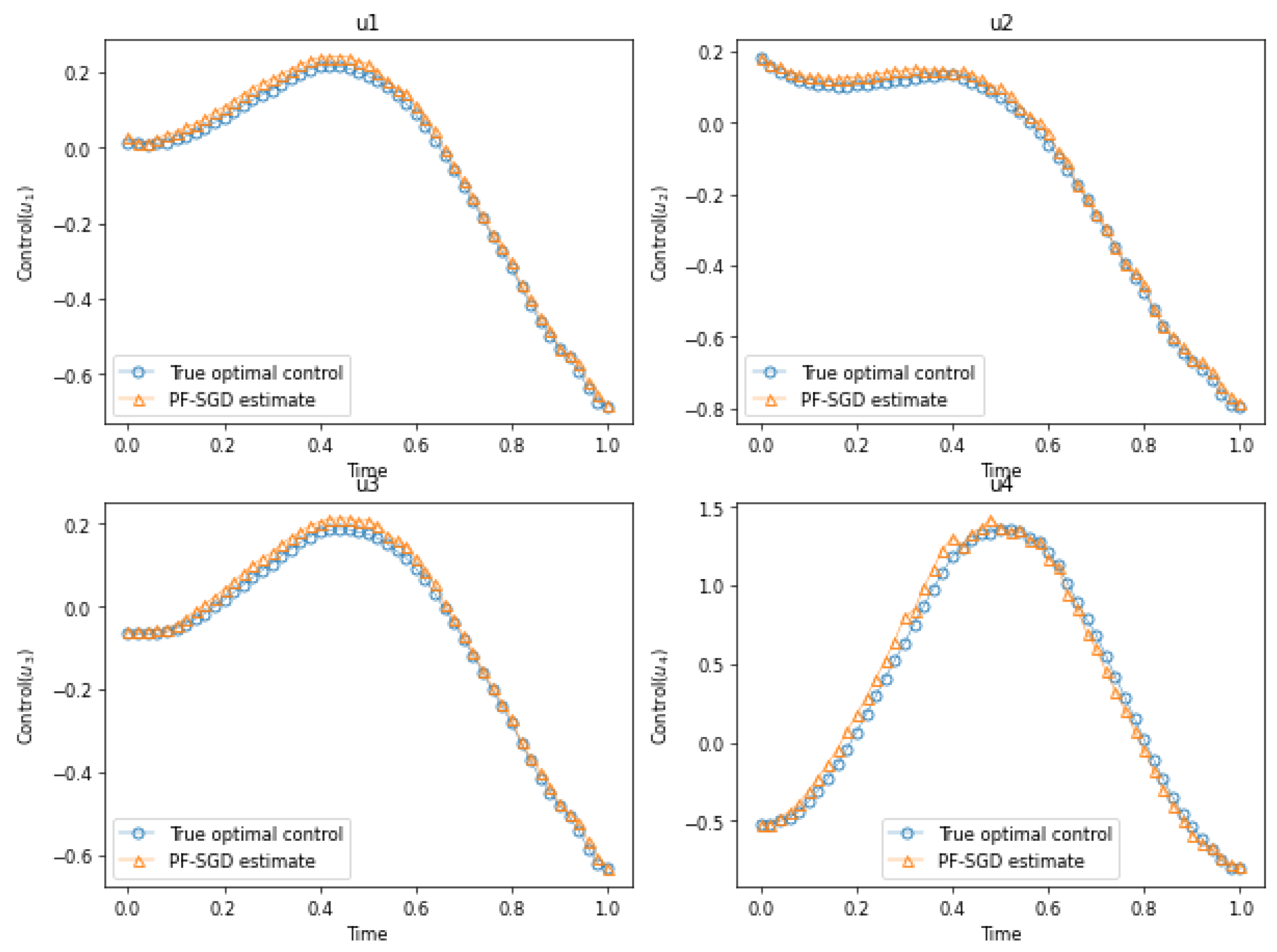
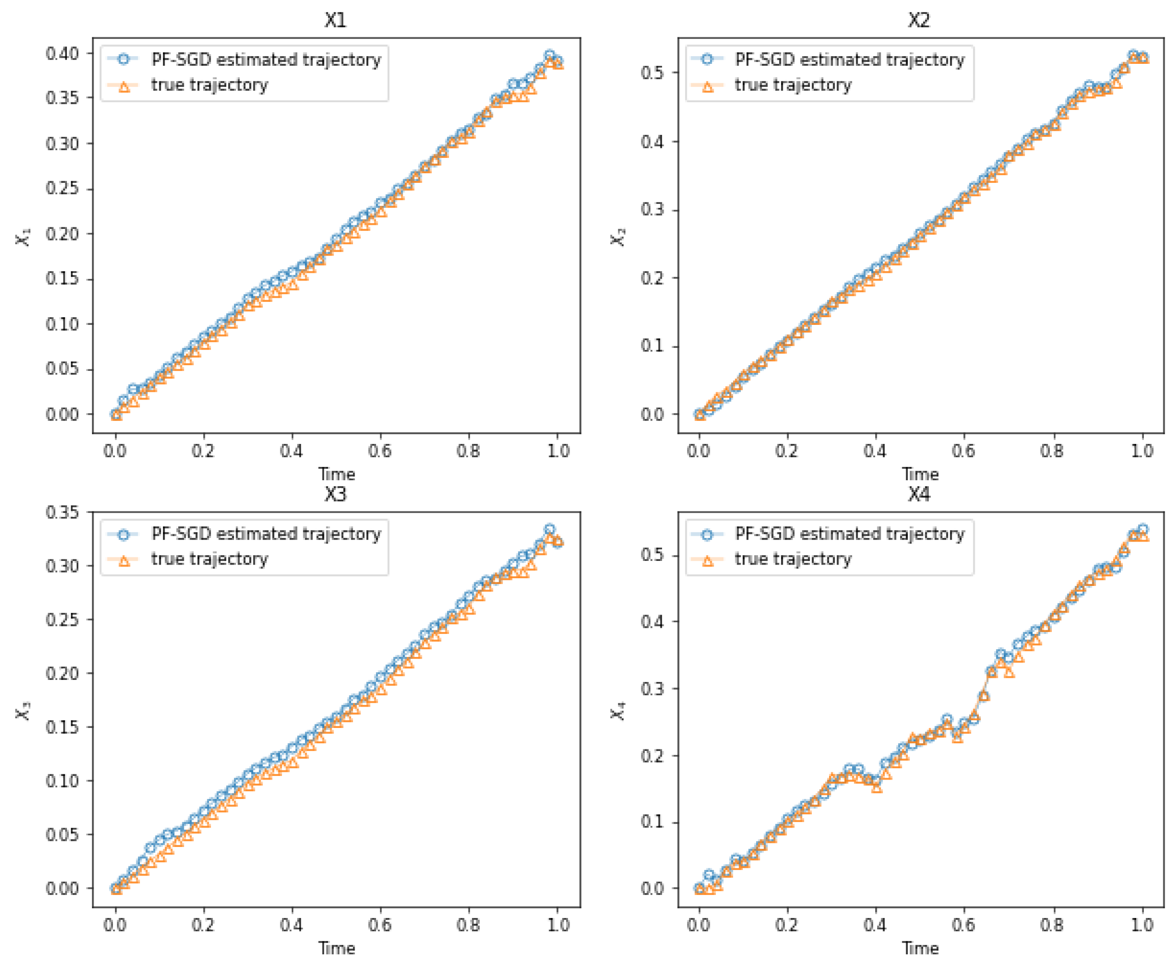
4.1.2. Performance Experiment

We set the total number of discretizations to be $N=50$. Set iteration $L={10}^4,\sigma =0.1$, the number of particles in each dimension is 128, $T=1$, and $X_0=0$.

In Figure 1, we present the estimated data-driven control and the true optimal control.

Figure 1. Estimated control vs. true optimal control.

In Figure 2, we show the estimated state trajectories with respect to true state trajectories in each dimension.

Figure 2. Estimated state vs. true state.

We can see from these Figures that our data-driven feedback control algorithm works very well for this 4-D linear quadratic control problem despite there being nonlinear observations.

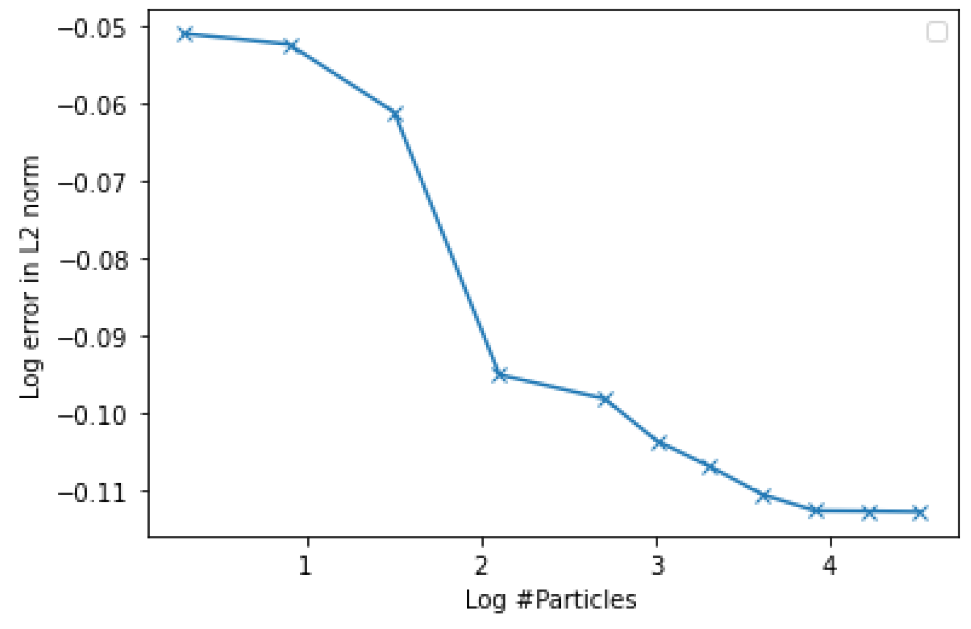
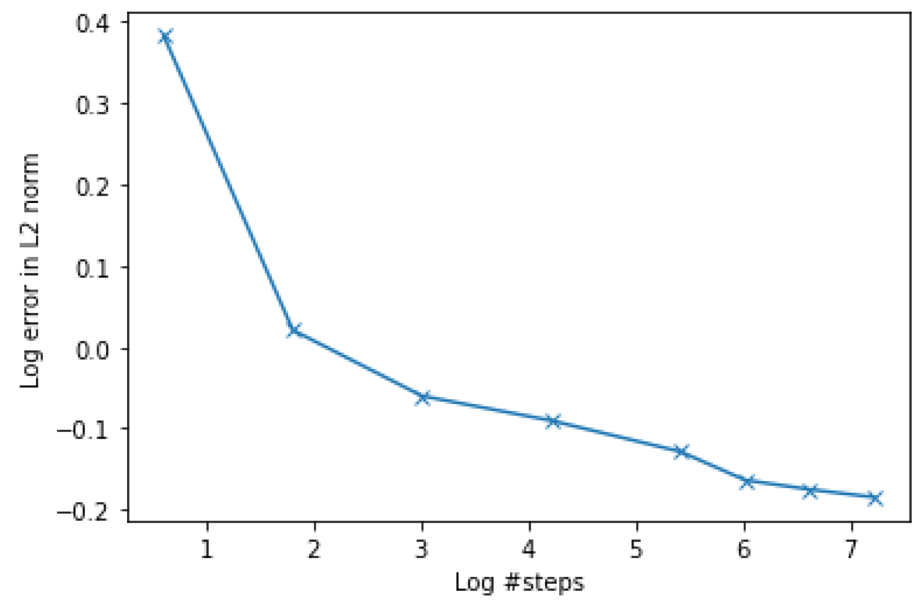
4.1.3. Convergence Experiment

In this experiment, we demonstrate the convergence performance of our algorithm, and we study the error decay of the algorithm in the $L_2$ norm with respect to the number of particles used. Each result is an average of $\left|\right|u^{est}-u^{*}{\left|\right|}_2$ of 50 independent tests.

Specifically, we set $L={10}^4$ and we just increase the number of particles S = {2, 8, 32, 128, 512, 2048, 4096, 8192, 16,384, 32,768}, and we obtained the result in Figure 3.

Figure 3. Error vs. number of particles.

Set the number of particles $S=\{2,8,32,128,512,1024,2048,4096\}$, and $L=S^2$. We obtained the result in Figure 4.

Figure 4. Error vs. number of steps.

From the results above, we can see that the error will decrease and converge as we increase the number of particles and the number of iterations.

4.2. Example 2. Two-Dimensional Dubins Vehicle Maneuvering Problem

In this example, we solve a Dubins vehicle maneuvering problem. The controlled process is described by the following nonlinear controlled dynamics:

$$\begin{array}{cc}\hfill d{S}_t& =\left[\begin{array}{c}d{X}_t\\ d{Y}_t\end{array}\right]=\left[\begin{array}{c}sin\left({\theta }_t\right)dt\\ cos\left({\theta }_t\right)dt\end{array}\right]+\sigma d{W}_t\hfill \end{array}$$

(104)

$$\begin{array}{cc}\hfill d{\theta }_t& =u_{t}dt+{\sigma }^{2}d{W}_t\hfill \end{array}$$

(105)

$$\begin{array}{cc}\hfill d{M}_t& ={[arctan\left({\displaystyle \frac{X_t+1}{Y_t-1}}\right),arctan\left({\displaystyle \frac{X_t-2}{Y_t-1}}\right)]}^T+{\eta }_t\hfill \end{array}$$

(106)

where the pair $(X,Y)$ gives the position of a car-like robot moving in the 2D plane, $\theta$ is the steering angle that controls the moving direction of the robot, which is governed by the control action $u_t$, and $\sigma$ is the noise that perturbs the motion and control actions. Assume that we do not have direct observations on the robot. Instead, we use two detectors located on different observation platforms at $(-1,1)$ and $(2,1)$ to collect bearing angles of the target robot as indirect observations. Thus, we have the observation process $M_t$. Given the expected path $S^{*}$, the car should follow it and arrive at the terminal position on time. The performance cost functional based on observational data that we aim to minimize is defined as:

$$J\left[u\right]=E\left[{\displaystyle \frac{1}{2}}{\int }_0^T⟨R(S_t-S_t^{*}),(S_t-S_t^{*})⟩dt+{\displaystyle \frac{1}{2}}{\int }_0^T⟨K{u}_t,u_t⟩dt+⟨Q(S_T-S_T^{*}),(S_T-S_T^{*})⟩\right]$$

(107)

In our numerical experiments, we let the car start from $(X_0,Y_0)=(0,0)$ to $(X_T,Y_T)=(1,1)$. The expected path $S_t^{*}$ is $X_t^2+Y_t^2=1$. Other settings are $T=1$, $\Delta t=0.02$, i.e., $N_T=50$, $\sigma =0.1$, ${\eta }_t\sim N(0,0.1)$, $L=1000$, $K=1$, and the initial heading direction is $\pi /2$. To emphasize the importance of following the expected path and arriving at the target location at the terminal time, let $R=Q=20$.

In Figure 5, we plot our algorithm’s designed trajectory and the estimated trajectory. We can see from this figure that the car moves towards the target along the designed path and is “on target” at the final time with a very small error.

Figure 5. Controlled trajectory from (0,0) to (1,1).

We set $L={10}^3$ and we just increase the number of particles $S=\{2,8,32,128,512,$$1024,2048,4096,8192,16384,32768\}$. To provide the convergence of our algorithm in solving this Dubins vehicle maneuvering problem, we repeated the above experiment 50 times and we obtained the error = ${\displaystyle \frac{1}{M_{rept.}}}{\sum }_{m=1}^{M_{rept.}}⟨(S_t-S_t^{*}),(S_t-S_t^{*})⟩$ in Figure 6 where $M_{rept.}=50$.

Figure 6. Error vs. number of particles.

Set the number of particles $S=\{8,16,32,64,128,256,512,1024\}$, and $L=S^2$. We obtained the error=${\displaystyle \frac{1}{M_{rept.}}}{\sum }_{m=1}^{M_{rept.}}$ $⟨(S_t-S_t^{*}),(S_t-S_t^{*})⟩$ in Figure 7, where the error is the average of $\left|\right|S_t-S_t^{*}{\left|\right|}_2$.

Figure 7. Error vs. number of steps.

From the results above, we can see that the error will decrease and converge as we increase the number of particles and the number of iterations.

5. Conclusions

In this paper, we present the weak convergence of the data-driven feedback control algorithm proposed in [1]. We do not discuss the convergence rate due to the challenge of determining the radius M of the compact subspace that bounds all particles $X_i$. However, in practice, given a terminal time T, one can use Monte Carlo simulations to find an M that satisfies a certain probability in Lemma 2. Our numerical experiments indicate that both the estimated control and estimated distribution converge at a rate related to the number of particles and iterations.

Future work can focus on analyzing the convergence rate and error bounds for a given state system. This will provide clarity on the number of particles and iterations required to achieve the desired estimation accuracy when applying the algorithm from [1].

Appendix A.1

Proof of Lemma 2.

Proof. 

We start with time $t_0$.

Step 1. Starting from $X_0\sim \xi$ with $\mathbb{E}\left[{\xi }^2\right]\le C_0$, and by fixing an arbitrary control $u_0$, we have for the prediction step:

$$\begin{array}{cc}\hfill \mathbb{E}\left[\right|X_1^{-}{|}^2]& =\mathbb{E}\left[\right|X_0+b(X_0,u_0)\Delta t+\sigma \left(X_0\right)\Delta W_0{|}^2]\hfill \\ \hfill & \le \mathbb{E}[(1+\Delta t)X_0^2+(1+{\displaystyle \frac{1}{\Delta t}})b^2{(\Delta t)}^2]+C_{\sigma }^2\Delta t\hfill \\ \hfill & \le (1+\Delta t)C_0^2+(C_b^2(\Delta t+1)+C_{\sigma }^2)\Delta t\hfill \\ \hfill & :=C_0^{-}\hfill \end{array}$$

(A1)

Step 2. We denote the distribution $\mathcal{L}\left(X_1^{-}\right)\sim {\pi }_{t_1|t_0}$, and then the particle method will perform a random resampling from such a distribution and obtain a random distribution

$$\begin{array}{c}\hfill {\displaystyle \frac{1}{\mathcal{N}}}\sum _{i=1}^{\mathcal{N}}{\delta }_{x_i\left(\omega \right)}:={\pi }_{t_1|t_0}^N\end{array}$$

(A2)

Hence, we have for $X\sim {\pi }_{t_1|t_0}^N$, taking the expectation where the expectation is taken over all randomness in the measure

$$\begin{array}{cc}\hfill \mathbb{E}\left[X^2\right]& =\mathbb{E}\left[\mathbb{E}\left[X^2\right|{\mathcal{G}}_1^{-}]\right]={\displaystyle \frac{\mathcal{N}}{\mathcal{N}}}\mathbb{E}\left[\mathbb{E}\left[x_1^2\right|{\mathcal{G}}_1^{-}]\right]=\mathbb{E}\left[{\tilde{X}}^2\right]\hfill \end{array}$$

(A3)

where $x_i\sim {\pi }_{t_1|t_0}$ are i.i.d random samples, ${\mathcal{G}}_0$ contains the sampling randomness and $\tilde{X}\sim {\pi }_{t_1|t_0}$. The conditional expectation is meant to show that all the particles $\xi$ are conditionally independent (since there is other randomness that has accumulated in the history if we want to apply this argument recursively.) Thus, by (A1)

$$\begin{array}{cc}\hfill \mathbb{E}\left[{\tilde{X}}^2\right]& \le C_0^{-}\hfill \end{array}$$

(A4)

Step 3. We now have the random measure ${\pi }_{t_1|t_0}^N$, and we proceed to the analysis step. We have by definition

$$\begin{array}{c}\hfill X_1\sim {\displaystyle \frac{g\left(x\right)d{\pi }_{t_1|t_0}^N\left(x\right)}{\int g\left(x\right)d{\pi }_{t_1|t_0}^N\left(x\right)}}:={\tilde{\pi }}_{t_1|t_1}^N\end{array}$$

(A5)

where ${\pi }_{t_1|t_0}^N\left(x\right)$ is the distribution of the terminal state $X_1^{-}$ from the previous step. Recalling assumption 7, we give an estimate over $\mathbb{E}\left[\right|X_1{|}^2]$:

$$\begin{array}{cc}\hfill \mathbb{E}\left[\right|X_1{|}^2]& \le {\left({\displaystyle \frac{1}{\kappa }}\right)}^2\mathbb{E}[\int x^{2}d{\pi }_{t_1|t_0}^N\left(x\right)]\le {\left({\displaystyle \frac{1}{\kappa }}\right)}^2{C}_0^{-}:=C_1\hfill \end{array}$$

(A6)

Step 4. Now, we again apply the random sampling step

$$\begin{array}{c}\hfill {\displaystyle \frac{1}{\mathcal{N}}}\sum _{i=1}^{\mathcal{N}}{\delta }_{x_i\left(\omega \right)}:={\pi }_{t_1|t_1}^N\end{array}$$

(A7)

where $x_i\left(\omega \right)\sim {\tilde{\pi }}_{t_1|t_1}^N$. Then, for $X\sim {\pi }_{t_1|t_1}^N$, we have

$$\begin{array}{cc}\hfill \mathbb{E}\left[X^2\right]& =\mathbb{E}\left[\mathbb{E}\left[X^2\right|{\mathcal{G}}_1]\right]\hfill \\ \hfill & ={\displaystyle \frac{\mathcal{N}}{\mathcal{N}}}\mathbb{E}\left[\mathbb{E}\left[x_i^2\right|{\mathcal{G}}_1]\right]\hfill \\ \hfill & =\mathbb{E}\left[{\tilde{X}}^2\right]\hfill \end{array}$$

(A8)

where $\tilde{X}\sim {\tilde{\pi }}_{t_1|t_1}^N$ and ${\mathcal{G}}_1$ is the filtration that builds on ${\mathcal{G}}_1^{-}$ and the randomness of the current sampling. Then, by (A6), we have

$$\begin{array}{c}\hfill \mathbb{E}\left[X^2\right]\le C_1,X\sim {\tilde{\pi }}_{t_1|t_1}^N\end{array}$$

(A9)

and this completes all the estimates for the first time-stepping. Hence, after one time step, we have

$$\begin{array}{c}\hfill C_1={\kappa }^{-2}(1+\Delta t)C_0+C\Delta t\end{array}$$

(A10)

which means that by applying the same argument, we will have the following recursion in general:

$$C_{n+1}={\kappa }^{-2}(1+\Delta t)C_n+C\Delta t$$

(A11)

As a result, by picking arbitrary $u_n$, using this same argument repeatedly until N, we have that for all $n=1,\dots ,N$:

$$\begin{array}{c}\hfill C_n={\left({\kappa }^{-2}(1+\Delta t)\right)}^n{C}_0+\sum _{i=0}^{n-1}{\left({\kappa }^{-2}(1+\Delta t)\right)}^{i}C\Delta t\end{array}$$

(A12)

and we notice that $C_n$ is increasing in n. As a result, we know that for any $X_n\sim {\pi }_{t_n|t_{n-1}}^N,{\pi }_{t_n|t_n}^N$, we have that

$$\begin{array}{c}\hfill \mathbb{E}\left[\right|X_n{|}^2]\le C_N\end{array}$$

(A13)

Hence, by Chebyshev’s inequality, we have

$$\begin{array}{c}\hfill \mathbb{P}\left(\right|X_n|\ge M)\le {\displaystyle \frac{C_N}{M^2}},\forall n\in \{1,2,\dots ,N\}\end{array}$$

(A14)

and then we have that

$$\begin{array}{c}\hfill \mathbb{P}(\underset{n}{sup}|X_n|\ge M)\le {\displaystyle \frac{C_N}{M^2}}\end{array}$$

(A15)

By noticing that the control values are arbitrarily picked, we have that

$$\begin{array}{c}\hfill \mathbb{P}(\underset{n,U_0}{sup}|X_n|\ge M)\le {\displaystyle \frac{C}{M^2}},X_n\sim {\pi }_{t_n|t_{n-1}}^N\mathit{or}{\pi }_{t_n|t_n}^N\end{array}$$

(A16)

□

References

- Archibald, R.; Bao, F.; Yong, J.; Zhou, T. An efficient numerical algorithm for solving data driven feedback control problems. J. Sci. Comput. 2020, 85, 51. [Google Scholar] [CrossRef]
- Bellman, R. Dynamic programming. Science 1966, 153, 34–37. [Google Scholar] [CrossRef] [PubMed]
- Feng, X.; Glowinski, R.; Neilan, M. Recent developments in numerical methods for fully nonlinear second order partial differential equations. SIAM Rev. 2013, 55, 205–267. [Google Scholar] [CrossRef]
- Peng, S. A general stochastic maximum principle for optimal control problems. SIAM J. Control Optim. 1990, 28, 966–979. [Google Scholar] [CrossRef]
- Yong, J.; Zhou, X.Y. Stochastic Controls: Hamiltonian Systems and HJB Equations; Springer Science & Business Media: Cham, Switzerland, 2012. [Google Scholar]
- Gong, B.; Liu, W.; Tang, T.; Zhao, W.; Zhou, T. An efficient gradient projection method for stochastic optimal control problems. SIAM J. Numer. Anal. 2017, 55, 2982–3005. [Google Scholar] [CrossRef]
- Tang, S. The maximum principle for partially observed optimal control of stochastic differential equations. SIAM J. Control Optim. 1998, 36, 1596–1617. [Google Scholar] [CrossRef]
- Zhang, J. A numerical scheme for BSDEs. Ann. Appl. Probab. 2004, 14, 459–488. [Google Scholar] [CrossRef]
- Zhao, W.; Fu, Y.; Zhou, T. New kinds of high-order multistep schemes for coupled forward backward stochastic differential equations. SIAM J. Sci. Comput. 2014, 36, A1731–A1751. [Google Scholar] [CrossRef]
- Archibald, R.; Bao, F.; Yong, J. A stochastic gradient descent approach for stochastic optimal control. East Asian J. Appl. Math. 2020, 10, 635–658. [Google Scholar] [CrossRef]
- Sato, I.; Nakagawa, H. Approximation analysis of stochastic gradient Langevin dynamics by using Fokker-Planck equation and Ito process. In Proceedings of the International Conference on Machine Learning, Beijing, China, 21–26 June 2014; Volume 32, pp. 982–990. [Google Scholar]
- Shapiro, A.; Wardi, Y. Convergence analysis of gradient descent stochastic algorithms. J. Optim. Theory Appl. 1996, 91, 439–454. [Google Scholar] [CrossRef]
- Archibald, R.; Bao, F.; Cao, Y.; Sun, H. Numerical analysis for convergence of a sample-wise backpropagation method for training stochastic neural networks. SIAM J. Numer. Anal. 2024, 62, 593–621. [Google Scholar] [CrossRef]
- Zakai, M. On the optimal filtering of diffusion processes. Z. Wahrscheinlichkeitstheorie Verw. Gebiete 1969, 11, 230–243. [Google Scholar] [CrossRef]
- Gordon, N.J.; Salmond, D.J.; Smith, A.F. Novel approach to nonlinear/non-Gaussian Bayesian state estimation. IEE Proc. F (Radar Signal Process.) 1993, 140, 107–113. [Google Scholar] [CrossRef]
- Morzfeld, M.; Tu, X.; Atkins, E.; Chorin, A.J. A random map implementation of implicit filters. J. Comput. Phys. 2012, 231, 2049–2066. [Google Scholar] [CrossRef]
- Andrieu, C.; Doucet, A.; Holenstein, R. Particle Markov chain Monte Carlo methods. J. R. Statist. Soc. B 2010, 72, 269–342. [Google Scholar] [CrossRef]
- Crisan, D.; Doucet, A. A survey of convergence results on particle filtering methods for practitioners. IEEE Trans. Signal Process. 2002, 50, 736–746. [Google Scholar] [CrossRef]
- Künsch, H.R. Particle filters. Bernoulli 2013, 19, 1391–1403. [Google Scholar] [CrossRef]
- Bao, F.; Cao, Y.; Meir, A.; Zhao, W. A first order scheme for backward doubly stochastic differential equations. SIAM/ASA J. Uncertain. Quantif. 2016, 4, 413–445. [Google Scholar] [CrossRef]
- Zhao, W.; Zhou, T.; Kong, T. High order numerical schemes for second-order FBSDEs with applications to stochastic optimal control. Commun. Comput. Phys. 2017, 21, 808–834. [Google Scholar] [CrossRef]
- Law, K.; Stuart, A.; Zygalakis, K. Data Assimilation; Springer: Cham, Switzerland, 2015. [Google Scholar]
Disclaimer/Publisher’s Note: The statements, opinions and data contained in all publications are solely those of the individual author(s) and contributor(s) and not of MDPI and/or the editor(s). MDPI and/or the editor(s) disclaim responsibility for any injury to people or property resulting from any ideas, methods, instructions or products referred to in the content. |
© 2024 by the authors. Licensee MDPI, Basel, Switzerland. This article is an open access article distributed under the terms and conditions of the Creative Commons Attribution (CC BY) license (https://creativecommons.org/licenses/by/4.0/).