
Process Capability Index for Simple Linear Profile in the Presence of Within- and Between-Profile Autocorrelation


Abstract
1. Introduction
- A functional capability index, denoted by in the absence of the autocorrelation effect, is introduced.
- In the presence of the BPAC effect, using the proposed method by Noorossana et al. [9], the index is modified to eliminate the autocorrelation effect.
- In the presence of the WPAC effect, the transformation method of Soleimani et al. [13] is used to eliminate the WPAC effect, and the index is modified accordingly to perform capability analysis for SLP.
- As the final and major contribution of this study, a novel method for analyzing the capability of SLP in the presence of both within- and between-profile autocorrelation is developed using the transformation approach proposed by Nadi et al. [18]. Then, the proposed PCI is modified to perform capability analysis for SLP.
2. Preliminaries
2.1. SLPs with a General Error Model
2.2. The Capability Index for Traditional SLP
2.3. Existing Process Yield Indices for SLP with BPAC and WPAC
2.3.1. Process Yield Index for SLP with BPAC
2.3.2. Process Yield Index for SLP with WPAC
3. The Proposed PCIs for Autocorrelated Linear Profiles
3.1. The Proposed PCI for SLP with BPAC
3.2. The Proposed PCI for SLP with WPAC
3.3. The Proposed PCI for SLP with BAC
4. Simulation Study
| Pseudocode 1. The procedure for computing , bias, and MSE using Monte Carlo simulation |
| Consider the in-control profile model, SLs’ function, sigma = 1, , , , and . errorpre = normrnd (0,sigma,[1,n]); % Normal preerror with size n while (we do not reach the number of generated samples) aij = normrnd (0,sigma,[1,n]); % Normal variable with size n % Generate data for i = 1:n if (i == 1) epsilon (i) = × errorpre (i) + aij (i); else epsilon(i) = × epsilon (i − 1) + × errorpre (i) − × × errorpre (i − 1) + aij (i); endif endfor + epsilon; % Equation (1) errorpre = epsilon; % Update the previous error endwhile % For the two autocorrelation structures, it is necessary to transfer the SLs as we apply the transformation of the in-control profile model. if (WPAC|BAC) % The details for computations were given in Section 3.2 and Section 3.3 Apply the transformation on the SLs. endif Compute based on Equation (10) and the in-control parameters. % The Monte Carlo simulation loop. % The computed in each iteration is denoted by . for rep = 1:1:10,000 Generate m profiles by the in-control model. % The parameter estimation is performed based on the autocorrelation structure. = Estimate the profile parameters including intercept, slope, and standard deviation based on the m profiles. Compute based on the proposed method for each category. = Estimate based on Equation (10) by and . Store the values endfor = . MSE = . bias = |
4.1. Simulation Study for SLP in the Presence of BPAC
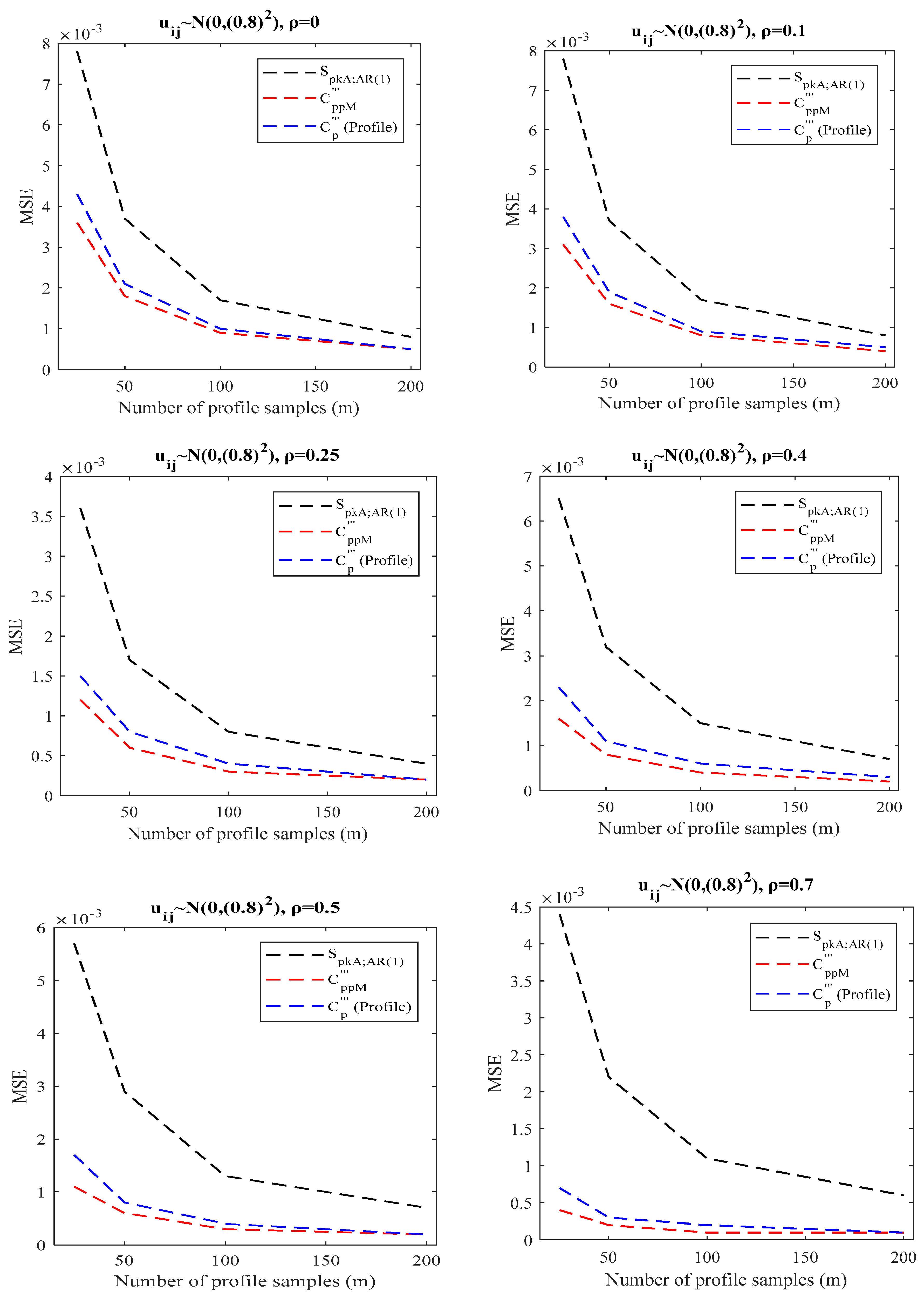
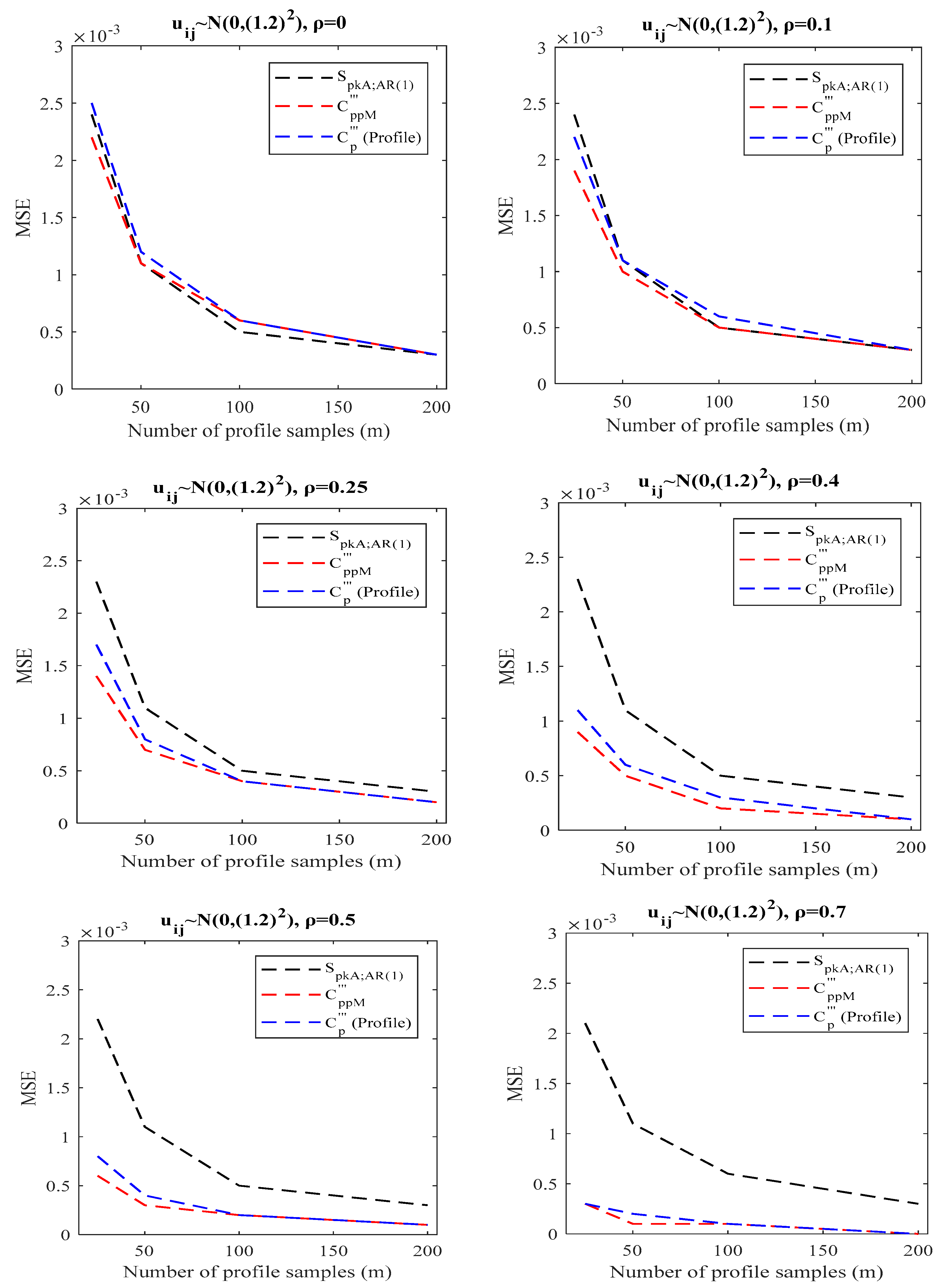
4.2. Simulation Study for SLP in the Presence of WPAC
4.3. Simulation Study for SLP in the Presence of BAC
4.4. Findings of the Simulation Studies
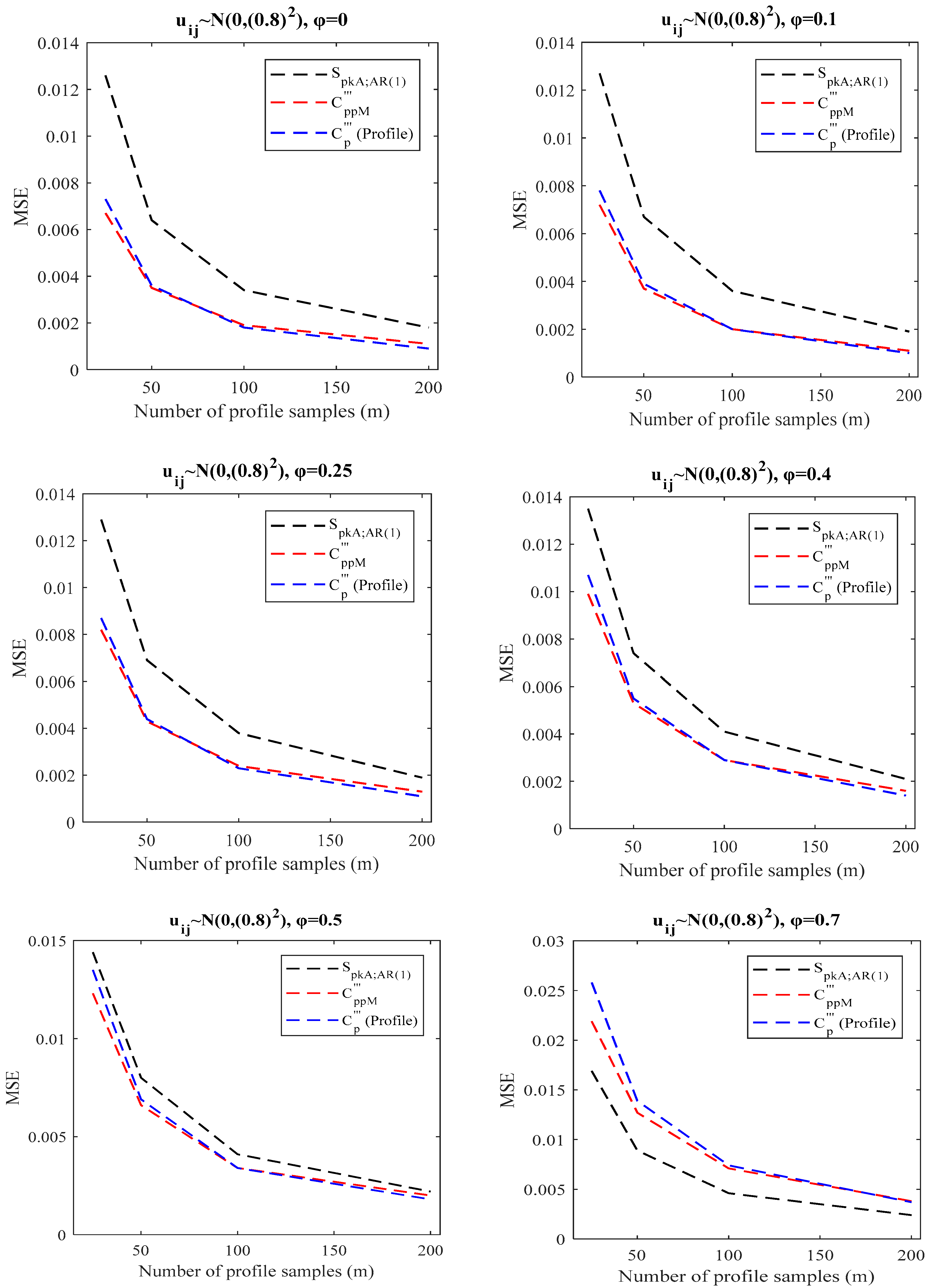
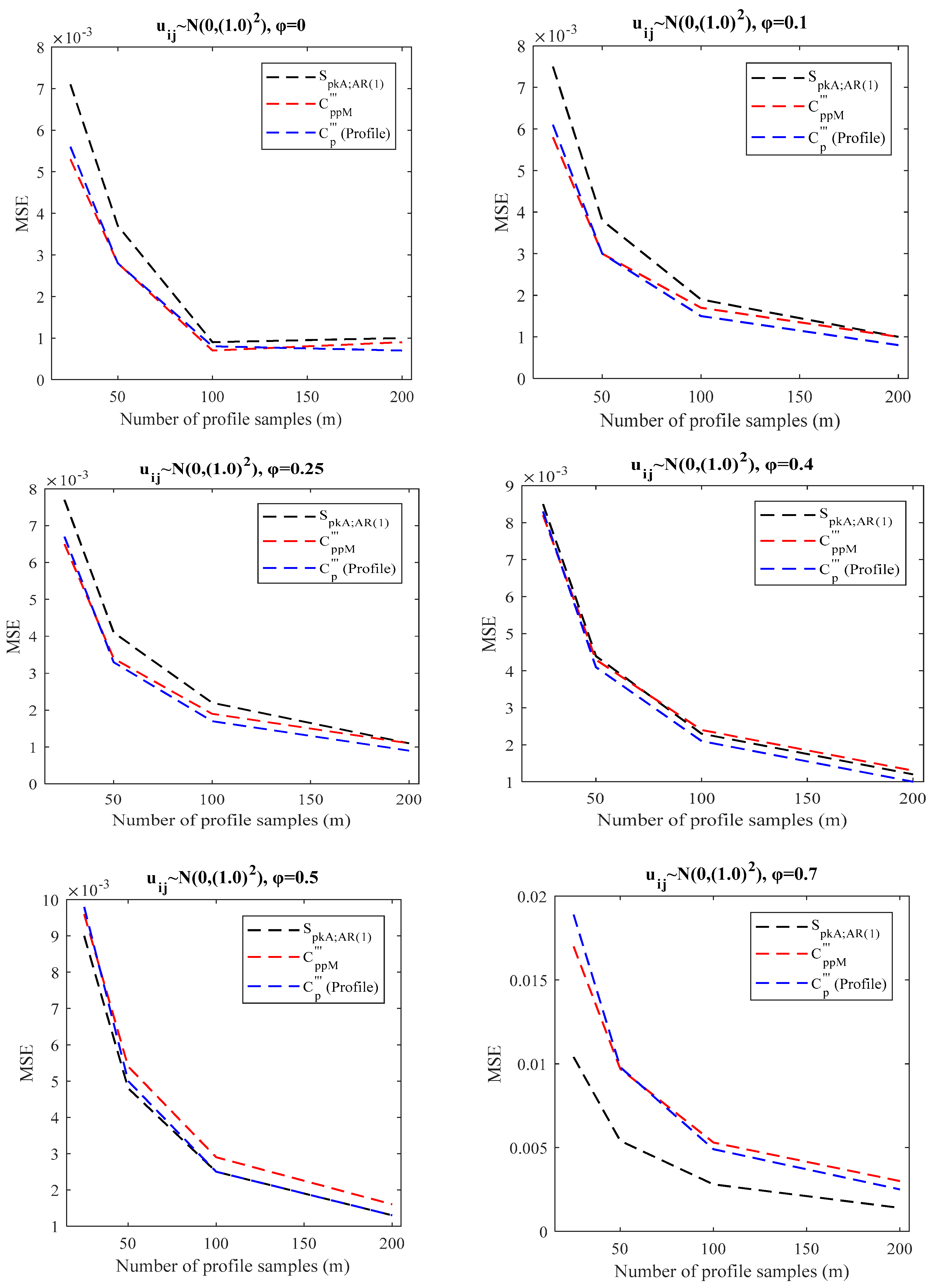
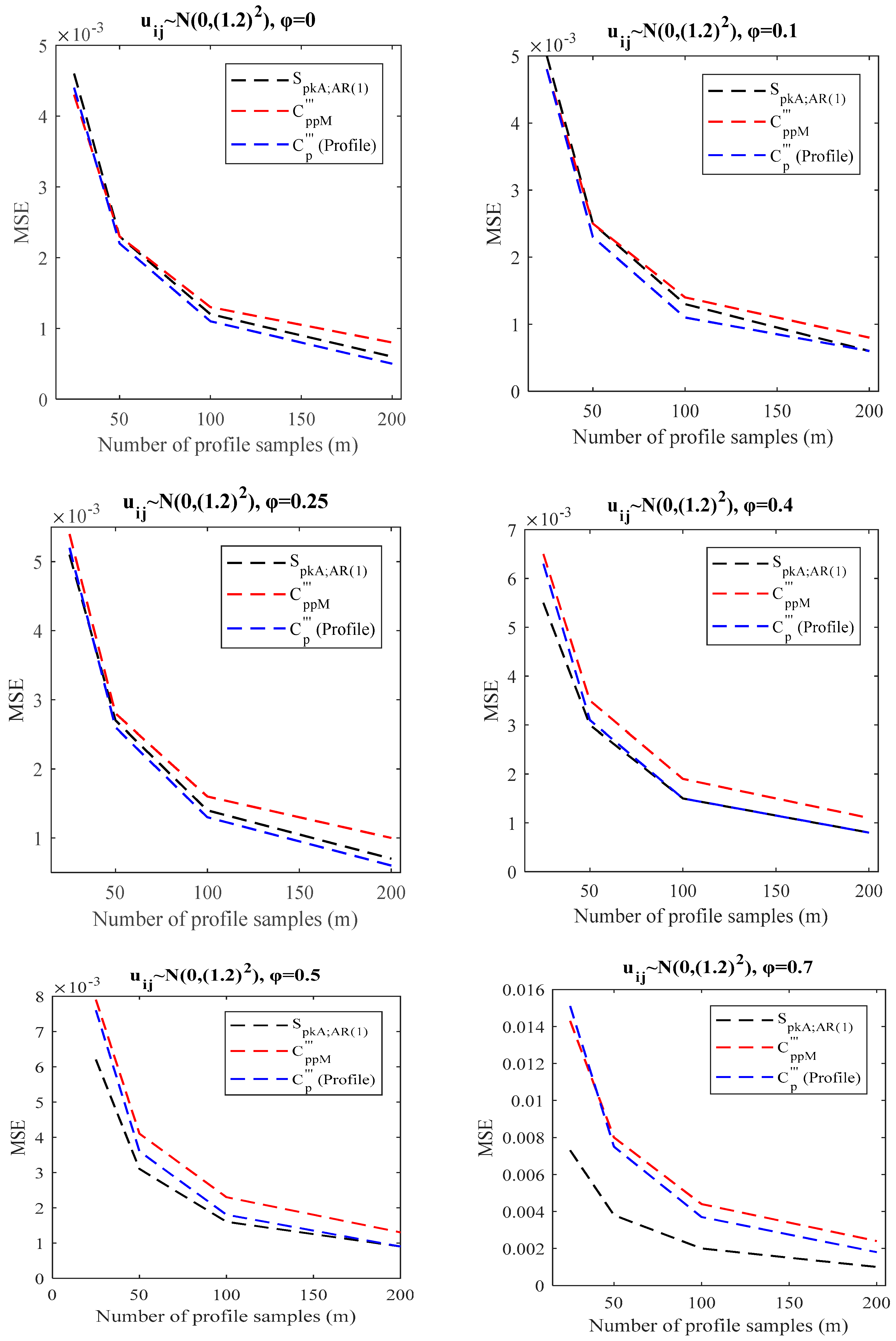
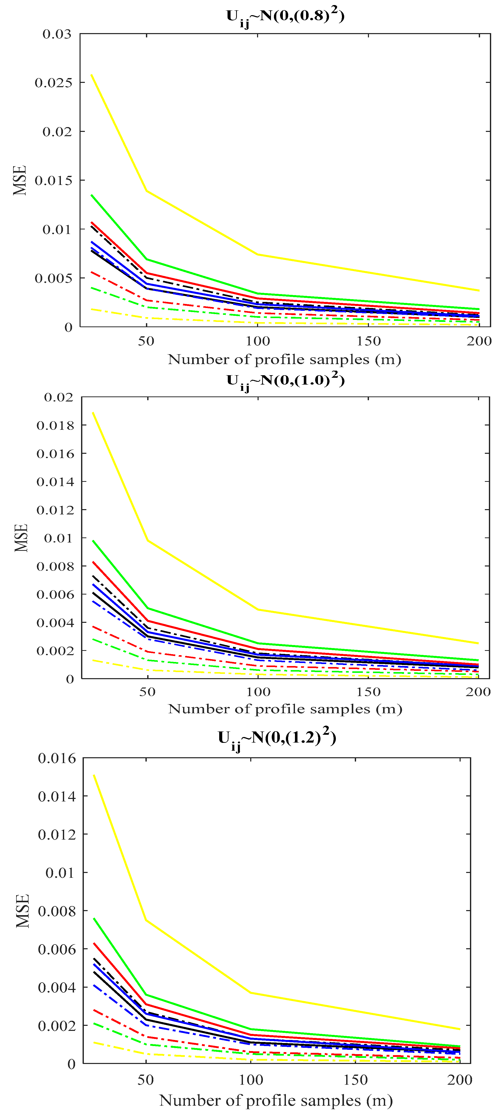
- When there is a BPAC effect (()), one can use the transformations in Section 3.1 and Section 3.3 as two options for recommending PCI. To select the superior transformation, a comparison between the proposed indices in Section 3.1 and Section 3.3 is provided. We conducted the same simulation studies in Section 4.1 () and calculated the proposed index in Section 3.3. Table 9 displays the outcomes of the simulations. Based on the simulation results in the last columns of Table 2, Table 3, Table 4 and Table 9, as well as Figure 7, as increases, the difference between the two methods becomes more apparent, and the proposed index in Section 3.3 outperforms the proposed index in Section 3.1, especially for with regard to bias and MSE criteria. Additionally, Figure 7 clearly shows these findings based on MSE criteria. Similarly, it can be observed that the suggested index in Section 3.3 generally has better bias and MSE than the index in Section 2.3.1 by comparing the first column of Table 2, Table 3 and Table 4 with the findings of Table 9. Thus, when there is a BPAC effect, we suggest using the proposed index discussed in Section 3.3.
- When there is a WPAC effect (), the proposed index in Section 3.2 can be used because the transformation method in Equation (22) reduces to Equation (20), and according to simulation results in Section 4.2, the index outperforms its competitors (see Table 5, Table 6 and Table 7 and Figure 4, Figure 5 and Figure 6).
- When there is a BAC effect (), the proposed index in Section 3.3 is recommended.
5. Bootstrap Confidence Intervals for in the Presence of BAC
5.1. Standard Bootstrap (SB) Confidence Interval
5.2. Percentile Bootstrap (PB) Confidence Interval
5.3. Simulation Study: Confidence Interval Evaluation
| Pseudocode 2. The procedure for computing the bootstrap confidence interval for , and relative coverage using Monte Carlo simulation |
| Consider the in-control profile model, SLs’ function, sigma = 1, , , , and .
errorpre = normrnd (0,sigma, [1,n]); % Normal preerror with size n while (we do not reach the number of generated samples) aij = normrnd (0,sigma,[1,n]); % Normal variable with size n % Generate data for i = 1:n if (i == 1) epsilon(i) = × errorpre(i) + aij(i); else epsilon(i) = × epsilon (i−1) + × errorpre(i) − × × errorpre (i−1) + aij(i); endif endfor + epsilon; % Equation (1) errorpre = epsilon; % Update the previous error endwhile % It is necessary to transfer the SLs as we apply the transformation of the in-control profile model.% The details for computations were given in Section 3.3. Apply the transformation on the SLs. Compute based on Equation (10) and the in-control parameters. for rep = 1:1:10,000 Generate m profiles by the in-control model. do a bootstrap loop 1000 times Generate a bootstrap with resampling profiles based on the m generated profile. % The parameter estimation is performed based on the computations given in Section 3.3. ) = Estimate the profile parameters, including intercept, slope, and standard deviation, based on the m profiles. Compute based on the proposed method for SLP with BAC. Estimate based on the Equation (10) by and , . Store the values . Sort from the smallest to largest. endloop = . Compute the SB and PB confidence intervals. Record the length of intervals. endfor Compute the average of 10,000 values. Compute the average of confidence intervals (). Compute the average interval length, coverage percentage, and relative coverage for the SB and PB approaches. |
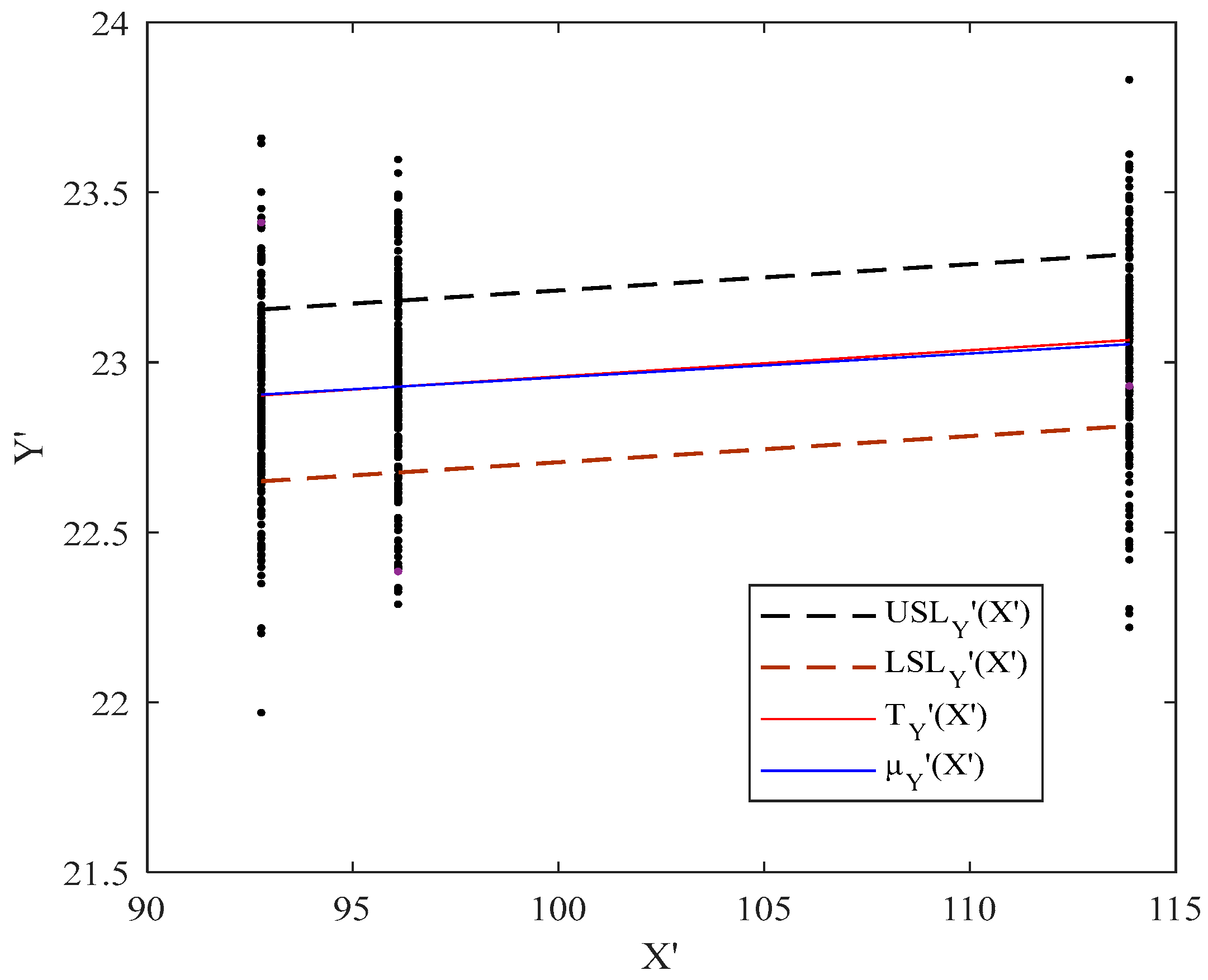
6. Illustrative Example
- Data Collection: Real-world data should be collected in accordance with appropriate sampling plans to ensure representativeness and statistical power.
- Data Preprocessing: Data cleaning and preprocessing steps are essential to address issues such as missing values, outliers, and trends.
- Parameter Estimation: The parameters of the autocorrelation models can be estimated using standard statistical methods, such as maximum likelihood or least squares.
- Phase I Profile Monitoring: The process stability should be assessed and the in-control profile parameters estimated.
- Process Capability Assessment: The proposed process capability index can be calculated based on the estimated parameters and the observed data.
- Interpretation: The results should be interpreted in the context of the specific application and used to inform decision making.
7. Conclusions and Future Works
- In the case of BPAC, the new index had a bias that was noticeably lower than the bias of the indices and for all the values of correlation coefficients , and its MSE was also lower than the MSE of especially for , and approximately equal to that of .
- In the case of WPAC, the new index outperformed the index due to its smaller bias and MSE in all simulated cases. In addition, the index performed better than due to its close MSE to the index and extremely small bias.
- In two cases, BPAC and WPAC, all PCIs performed well with a larger sample size.
Author Contributions
Funding
Data Availability Statement
Conflicts of Interest
Appendix A
- Calculating the true values of : By considering , , , , and , Equation (6) is used to first determine the values of for 4 levels of the explanatory variable, which are calculated as 1.3008, 1.4401, 1.5547, and 1.2015, respectively. The values of are then calculated using Equation (7) and are equal to 0.9999, 1, 1, and 0.9997. Therefore, value is calculated, which is equal to 0.9999. Using Equation (8), the index is finally calculated to be 1.2916.
- Calculating the true value of : By considering , , , , and , we must first calculate the values of for each of the 4 levels of the explanatory variable using Equation (4). These values are 1.0943, 1.3816, 1.5625, and 0.9067, respectively. Finally, the is calculated to be 1.2363.
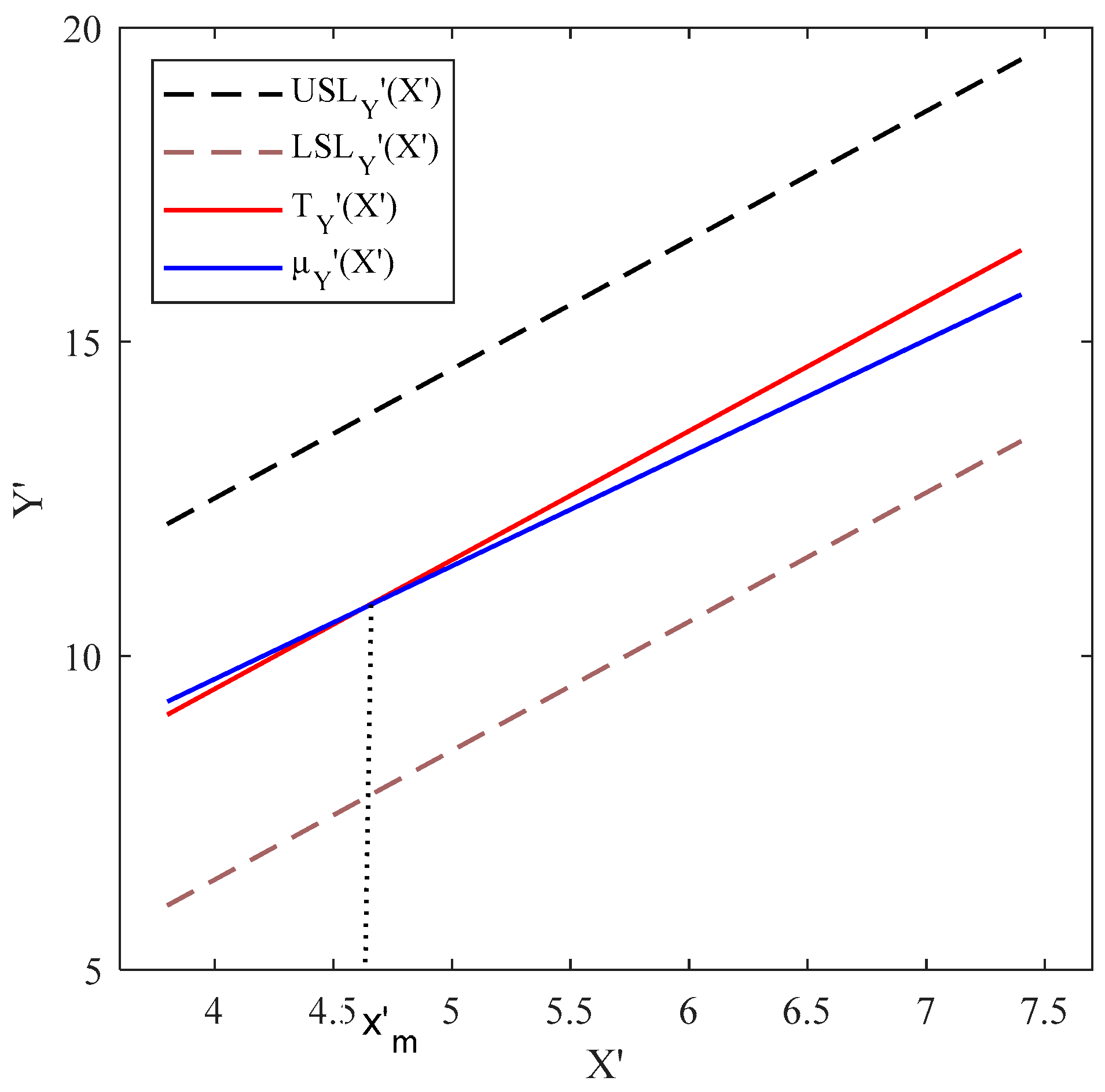
- Calculating the true value of : By considering , , , , and , firstly, the regression lines are fitted to the values of , , and , to yield the functional SLs and target line as , , and , where . Then, to calculate , the location of relative to is determined based on the method proposed in Pakzad and Basiri [39]. Figure A1 shows that and cross at and is calculated as 1.3160 using Equation (16).

Appendix B
- Calculating the true values of : By considering , , , , and , first Equation (6) is used to calculate the values of for 10 levels of the explanatory variable as 1.1344, 1.3008, 1.3566, 1.4401, 1.5517, 1.5547, 1.3964, 1.2015, 1.1738, and 1.4975, respectively. The values of are then calculated using Equation (7) as 0.9993, 0.9999, 1, 1, 1, 1, 1, 0.9997, 0.9996, and 1. is thus calculated to be 0.9998. Using Equation (8), the index is finally calculated to be 1.2579.
- Calculating the true value of : By considering , , , , and , first the transformation method of Soleimani et al. [13] is applied. Therefore, we have , , , , and . The values of for 9 levels of are then determined using Equation (4) as 1.0640, 1.1396, 1.2817, 1.4061, 1.4064, 1.1587, 0.8347, 0.8208, and 1.3818, respectively. The is finally calculated as 1.1660.
- Calculating the true value of : By considering , , , , and , as well as using the transformation method proposed by Soleimani et al. [13], we obtain , , , , and . Then, the regression lines are fitted to the values of , , and , to obtain the functional transformed SLs and target line as , , and , where . Finally, to calculate , the location of relative to is determined based on the method proposed in Pakzad and Basiri [39]. As we can see in Figure A2, and , intersect at and derived as 1.2238 based on Equation (16).

Appendix C
- Calculating the true value of : By considering , , , , and , the regression lines are first fitted to the values of , , and , resulting in the functional SLs and target line as , , and , where . Then the transformation by Soleimani et al. [13] is used. According to Equation (22), , , and , and , where . Then, to calculate , the location of relative to is determined based on the method proposed in Pakzad and Basiri [39]. Figure A3 demonstrates that and intersect at and obtained as 1.1387 based on Equation (16).
References
- Gupta, S.; Montgomery, D.C.; Woodall, W.H. Performance evaluation of two methods for online monitoring of linear calibration profiles. Int. J. Prod. Res. 2006, 44, 1927–1942. [Google Scholar] [CrossRef]
- Kang, L.; Albin, S.L. On-Line Monitoring When the Process Yields a Linear Profile. J. Qual. Technol. 2000, 32, 418–426. [Google Scholar] [CrossRef]
- Kim, K.; Mahmoud, M.A.; Woodall, W.H. On the Monitoring of Linear Profiles. J. Qual. Technol. 2003, 35, 317–328. [Google Scholar] [CrossRef]
- Li, Z.; Wang, Z. An exponentially weighted moving average scheme with variable sampling intervals for monitoring linear profiles. Comput. Ind. Eng. 2010, 59, 630–637. [Google Scholar] [CrossRef]
- Xu, L.; Wang, S.; Peng, Y.; Morgan, J.P.; Reynolds, M.R.; Woodall, W.H. The Monitoring of Linear Profiles with a GLR Control Chart. J. Qual. Technol. 2012, 44, 348–362. [Google Scholar] [CrossRef]
- Chen, S.; Yu, J.; Wang, S. Monitoring of complex profiles based on deep stacked denoising autoencoders. Comput. Ind. Eng. 2020, 143, 106402. [Google Scholar] [CrossRef]
- Nassar, S.H.; Abdel-Salam, A.-S.G. Robust profile monitoring for phase II analysis via residuals. Qual. Reliab. Eng. Int. 2022, 38, 432–446. [Google Scholar] [CrossRef]
- Maleki, M.R.; Amiri, A.; Castagliola, P. An overview on recent profile monitoring papers (2008–2018) based on conceptual classification scheme. Comput. Ind. Eng. 2018, 126, 705–728. [Google Scholar] [CrossRef]
- Noorossana, R.; Amiri, A.; Soleimani, P. On the Monitoring of Autocorrelated Linear Profiles. Commun. Stat. Theory Methods 2008, 37, 425–442. [Google Scholar] [CrossRef]
- Wang, Y.-H.T.; Huang, W.-H. Phase II monitoring and diagnosis of autocorrelated simple linear profiles. Comput. Ind. Eng. 2017, 112, 57–70. [Google Scholar] [CrossRef]
- Khedmati, M.; Niaki, S.T.A. Phase II monitoring of general linear profiles in the presence of between-profile autocorrelation. Qual. Reliab. Eng. Int. 2016, 32, 443–452. [Google Scholar] [CrossRef]
- Wang, Y.-H.T.; Lai, Y. Monitoring of autocorrelated general linear profiles. J. Stat. Comput. Simul. 2019, 89, 519–535. [Google Scholar] [CrossRef]
- Soleimani, P.; Noorossana, R.; Amiri, A. Simple linear profiles monitoring in the presence of within profile autocorrelation. Comput. Ind. Eng. 2009, 57, 1015–1021. [Google Scholar] [CrossRef]
- Jensen, W.A.; Birch, J.B.; Woodall, W.H. Monitoring Correlation Within Linear Profiles Using Mixed Models. J. Qual. Technol. 2008, 40, 167–183. [Google Scholar] [CrossRef]
- Zhang, W.; Niu, Z.; He, Z.; He, S. Online monitoring of profiles via function-on-scalar model with an application to industrial busbar. Qual. Reliab. Eng. Int. 2022, 38, 3816–3828. [Google Scholar] [CrossRef]
- Niaki, S.T.A.; Khedmati, M.; Soleymanian, M.E. Statistical Monitoring of Autocorrelated Simple Linear Profiles Based on Principal Components Analysis. Commun. Stat. Theory Methods 2015, 44, 4454–4475. [Google Scholar] [CrossRef]
- Yeganeh, A.; Johannssen, A.; Chukhrova, N.; Abbasi, S.A.; Pourpanah, F. Employing machine learning techniques in monitoring autocorrelated profiles. Neural Comput. Appl. 2023, 35, 16321–16340. [Google Scholar] [CrossRef]
- Nadi, A.A.; Yeganeh, A.; Shadman, A. Monitoring simple linear profiles in the presence of within-and between-profile autocorrelation. Qual. Reliab. Eng. Int. 2023, 39, 752–775. [Google Scholar] [CrossRef]
- Alevizakos, V. Process Capability and Performance Indices for Discrete Data. Mathematics 2023, 11, 3457. [Google Scholar] [CrossRef]
- Perakis, M.; Xekalaki, E. On the relationship between process capability indices and the proportion of conformance. Qual. Technol. Quant. Manag. 2016, 13, 207–220. [Google Scholar] [CrossRef]
- Afshari, R.; Nadi, A.A.; Johannssen, A.; Chukhrova, N.; Tran, K.P. The effects of measurement errors on estimating and assessing the multivariate process capability with imprecise characteristic. Comput. Ind. Eng. 2022, 172, 108563. [Google Scholar] [CrossRef]
- Wang, S.; Chiang, J.-Y.; Tsai, T.-R.; Qin, Y. Robust process capability indices and statistical inference based on model selection. Comput. Ind. Eng. 2021, 156. [Google Scholar] [CrossRef]
- Alevizakos, V.; Koukouvinos, C. Evaluation of process capability in gamma regression profiles. Commun. Stat. Simul. Comput. 2022, 51, 5174–5189. [Google Scholar] [CrossRef]
- Guevara G, R.D.; Alejandra Lopez, T. Process capability vector for multivariate nonlinear profiles. J. Stat. Comput. Simul. 2022, 92, 1292–1321. [Google Scholar] [CrossRef]
- Wang, F.K.; Guo, Y.C. Measuring process yield for nonlinear profiles. Qual. Reliab. Eng. Int. 2014, 30, 1333–1339. [Google Scholar] [CrossRef]
- Bera, K.; Anis, M.Z. Process incapability index for autocorrelated data in the presence of measurement errors. Commun. Stat. Theory Methods 2023, 53, 5439–5459. [Google Scholar] [CrossRef]
- Cohen, A.; Amin, R. The effects of normal mixtures and autocorrelation on the fraction non-conforming. Commun. Stat. Simul. Comput. 2017, 46, 8105–8117. [Google Scholar] [CrossRef]
- Lundkvist, P.; Vannman, K.; Kulahci, M. A comparison of decision method for Cpk when data are autocorrelated. Qual. Control. Appl. Stat. 2013, 58, 451–452. [Google Scholar]
- Hosseinifard, S.Z.; Abbasi, B. Evaluation of process capability indices of linear profiles. Int. J. Qual. Reliab. Manag. 2012, 29, 162–176. [Google Scholar] [CrossRef]
- Hosseinifard, S.Z.; Abbasi, B. Process Capability Analysis in Non Normal Linear Regression Profiles. Commun. Stat. Simul. Comput. 2012, 41, 1761–1784. [Google Scholar] [CrossRef]
- Ebadi, M.; Shahriari, H. A process capability index for simple linear profile. Int. J. Adv. Manuf. Technol. 2013, 64, 857–865. [Google Scholar] [CrossRef]
- Wang, F.-K. A Process Yield for Simple Linear Profiles. Qual. Eng. 2014, 26, 311–318. [Google Scholar] [CrossRef]
- Wang, F. Measuring the Process Yield for Simple Linear Profiles with one-Sided Specification. Qual. Reliab. Eng. Int. 2014, 30, 1145–1151. [Google Scholar] [CrossRef]
- Wang, F.-K.; Tamirat, Y. Process yield analysis for autocorrelation between linear profiles. Comput. Ind. Eng. 2014, 71, 50–56. [Google Scholar] [CrossRef]
- Wang, F.; Tamirat, Y. Process Yield Analysis for Linear Within-Profile Autocorrelation. Qual. Reliab. Eng. Int. 2015, 31, 1053–1061. [Google Scholar] [CrossRef]
- Mehri, S.; Ahmadi, M.M.; Shahriari, H.; Aghaie, A. Robust process capability indices for multiple linear profiles. Qual. Reliab. Eng. Int. 2021, 37, 3568–3579. [Google Scholar] [CrossRef]
- Ganji, Z.A.; Gildeh, B.S. A new process capability index for simple linear profile. Commun. Stat. Theory Methods 2023, 52, 3879–3894. [Google Scholar] [CrossRef]
- Pakzad, A.; Razavi, H.; Gildeh, B.S. Developing loss-based functional process capability indices for simple linear profile. J. Stat. Comput. Simul. 2022, 92, 115–144. [Google Scholar] [CrossRef]
- Pakzad, A.; Basiri, E. A new incapability index for simple linear profile with asymmetric tolerances. Qual. Eng. 2023, 35, 324–340. [Google Scholar] [CrossRef]
- Ganji, Z.A.; Gildeh, B.S. A class of process capability indices for asymmetric tolerances. Qual. Eng. 2016, 28, 441–454. [Google Scholar] [CrossRef]
- Boyles, R.A. Brocess capability with asymmetric tolerances. Commun. Stat. Simul. Comput. 1994, 23, 615–635. [Google Scholar] [CrossRef]
- Bothe, D.R. Measuring Process Capability: Techniques and Calculations for Quality and Manufacturing Engineers; McGraw-Hill Companies: New York, NY, USA, 1997. [Google Scholar]
- Keshteli, R.N.; Kazemzadeh, R.B.; Amiri, A.; Noorossana, R. Developing functional process capability indices for simple linear profile. Sci. Iran. 2014, 21, 1096–1104. [Google Scholar]
- Efron, B. The Jackknife, the Bootstrap and other Resampling Plans; SIAM: Philadelphia, PA, USA, 1982. [Google Scholar]
- Efron, B.; Tibshirani, R. Bootstrap Methods for Standard Errors, Confidence Intervals, and Other Measures of Statistical Accuracy. Stat. Sci. 1986, 1, 54–75. [Google Scholar] [CrossRef]
- Abbas, T.; Mahmood, T.; Riaz, M.; Abid, M. Improved linear profiling methods under classical and Bayesian setups: An application to chemical gas sensors. Chemom. Intell. Lab. Syst. 2020, 196, 103908. [Google Scholar] [CrossRef]
- Mahmood, T.; Riaz, M.; Omar, M.H.; Xie, M. Alternative methods for the simultaneous monitoring of simple linear profile parameters. Int. J. Adv. Manuf. Technol. 2018, 97, 2851–2871. [Google Scholar] [CrossRef]


| 1 | 2 | 3 | 4 | 5 | 6 | 7 | 8 | 9 | 10 | |
| 1 | 2 | 3 | 4 | 5 | 6 | 7 | 8 | 9 | 10 | |
| 0.08 | 2.5 | 4.64 | 6.85 | 9.2 | 11.25 | 13.76 | 16.25 | 18.32 | 19.5 | |
| 7.58 | 10 | 12.14 | 14.35 | 16.7 | 18.75 | 21.26 | 23.75 | 25.82 | 27 | |
| 3.83 | 6.25 | 8.39 | 10.6 | 12.95 | 15 | 17.51 | 20 | 22.07 | 23.25 |
| True Value | Estimate (Bias, MSE) | True Value | Estimate (Bias, MSE) | True Value | Estimate (Bias, MSE) | ||
|---|---|---|---|---|---|---|---|
| 0 | 25 | 1.2971 | 1.2589 (−0.0382, 0.0126) | 1.2363 | 1.2184 (−0.0179, 0.0067) | 1.3160 | 1.3162 (0.0002, 0.0073) |
| 50 | 1.2780 (−0.0191, 0.0064) | 1.2193 (−0.0170, 0.0035) | 1.3166 (0.0006, 0.0036) | ||||
| 100 | 1.2867 (−0.0104, 0.0034) | 1.2190 (−0.0173, 0.0019) | 1.3158 (−0.0002, 0.0018) | ||||
| 200 | 1.2917 (−0.0054, 0.0018) | 1.2187 (−0.0176, 0.0011) | 1.3154 (−0.0006, 0.0009) | ||||
| 0.1 | 25 | 1.2916 | 1.2576 (−0.0340, 0.0127) | 1.2363 | 1.2180 (−0.0183, 0.0072) | 1.3160 | 1.3151 (−0.0009, 0.0078) |
| 50 | 1.2738 (−0.0178, 0.0067) | 1.2190 (−0.0173, 0.0037) | 1.3158 (−0.0002, 0.0039) | ||||
| 100 | 1.2826 (−0.0090, 0.0036) | 1.2194 (−0.0169, 0.0020) | 1.3160 (0.0000, 0.0020) | ||||
| 200 | 1.2880 (−0.0036, 0.0019) | 1.2198 (−0.0165, 0.0011) | 1.3163 (0.0003, 0.0010) | ||||
| 0.25 | 25 | 1.2624 | 1.2328 (−0.0296, 0.0129) | 1.2363 | 1.2152 (−0.0211, 0.0082) | 1.3160 | 1.3107 (0.0053, 0.0087) |
| 50 | 1.2461 (−0.0163, 0.0069) | 1.2182 (−0.0181, 0.0043) | 1.3141 (0.0019, 0.0044) | ||||
| 100 | 1.2540 (−0.0084, 0.0038) | 1.2184 (−0.0179, 0.0024) | 1.3145 (−0.0015, 0.0023) | ||||
| 200 | 1.2582 (−0.0042, 0.0019) | 1.2190 (−0.0173, 0.0013) | 1.3154 (−0.0006, 0.0011) | ||||
| 0.4 | 25 | 1.2058 | 1.1858 (−0.0200, 0.0135) | 1.2363 | 1.2148 (−0.0215, 0.0099) | 1.3160 | 1.3077 (0.0083, 0.0107) |
| 50 | 1.1944 (−0.0114, 0.0074) | 1.2177 (−0.0186, 0.0053) | 1.3120 (0.0040, 0.0055) | ||||
| 100 | 1.1986 (−0.0072, 0.0041) | 1.2186 (−0.0177, 0.0029) | 1.3139 (−0.0021, 0.0029) | ||||
| 200 | 1.2019 (−0.0039, 0.0021) | 1.2188 (−0.0175, 0.0016) | 1.3148 (−0.0012, 0.0014) | ||||
| 0.5 | 25 | 1.1503 | 1.1391 (−0.0112, 0.0144) | 1.2363 | 1.2130 (−0.0233, 0.0123) | 1.3160 | 1.3027 (−0.0133, 0.0135) |
| 50 | 1.1424 (−0.0079, 0.0080) | 1.2178 (−0.0185, 0.0066) | 1.3104 (−0.0056, 0.0069) | ||||
| 100 | 1.1450 (−0.0053, 0.0041) | 1.2187 (−0.0176, 0.0034) | 1.3129 (−0.0031, 0.0034) | ||||
| 200 | 1.1466 (−0.0037, 0.0022) | 1.2187 (−0.0176, 0.0020) | 1.3138 (−0.0022, 0.0018) | ||||
| 0.7 | 25 | 0.9802 | 0.9974 (0.0172, 0.0169) | 1.2363 | 1.1995 (−0.0368, 0.0219) | 1.3160 | 1.2742 (−0.0418, 0.0258) |
| 50 | 0.9840 (0.0038, 0.0089) | 1.2095 (−0.0268, 0.0127) | 1.2934 (−0.0226, 0.0139) | ||||
| 100 | 0.9788 (−0.0014, 0.0046) | 1.2139 (−0.0224, 0.0071) | 1.3035 (−0.0125, 0.0074) | ||||
| 200 | 0.9792 (−0.0010, 0.0024) | 1.2174 (−0.0189, 0.0038) | 1.3101 (−0.0059, 0.0037) | ||||
| True Value | Estimated (Bias, MSE) | True Value | Estimated (Bias, MSE) | True Value | Estimated (Bias, MSE) | ||
|---|---|---|---|---|---|---|---|
| 0 | 25 | 1.0771 | 1.0488 (−0.0283, 0.0071) | 1.0446 | 1.0254 (−0.0192, 0.0053) | 1.1048 | 1.1042 (−0.0006, 0.0056) |
| 50 | 1.0629 (−0.0142, 0.0037) | 1.0270 (−0.0176, 0.0028) | 1.1050 (0.0002, 0.0028) | ||||
| 100 | 1.0696 (−0.0075, 0.0009) | 1.0270 (−0.0176, 0.0007) | 1.1048 (0.0000, 0.0008) | ||||
| 200 | 1.0738 (−0.0033, 0.0010) | 1.0275 (−0.0171, 0.0009) | 1.1050 (0.0002, 0.0007) | ||||
| 0.1 | 25 | 1.0726 | 1.0474 (−0.0252, 0.0075) | 1.0446 | 1.0251 (−0.0195, 0.0058) | 1.1048 | 1.1032 (0.0016, 0.0061) |
| 50 | 1.0581 (−0.0145 0.0038) | 1.0260 (−0.0186, 0.0030) | 1.1039 (−0.0009, 0.0030) | ||||
| 100 | 1.0655 (−0.0071, 0.0019) | 1.0269 (−0.0177, 0.0017) | 1.1045 (−0.0003, 0.0015) | ||||
| 200 | 1.0686 (−0.0040, 0.0010) | 1.0267 (−0.0179, 0.0010) | 1.1042 (−0.0006, 0.0008) | ||||
| 0.25 | 25 | 1.0486 | 1.0270 (−0.0216, 0.0077) | 1.0446 | 1.0230 (−0.0216, 0.0065) | 1.1048 | 1.0998 (−0.0050, 0.0067) |
| 50 | 1.0375 (−0.0111, 0.0041) | 1.0261 (−0.0185, 0.0034) | 1.1030 (−0.0018, 0.0033) | ||||
| 100 | 1.0424 (−0.0062, 0.0022) | 1.0265 (−0.0181, 0.0019) | 1.1037 (−0.0011, 0.0017) | ||||
| 200 | 1.0459 (−0.0027, 0.0011) | 1.0273 (−0.0173, 0.0011) | 1.1045 (−0.0003, 0.0009) | ||||
| 0.4 | 25 | 1.0019 | 0.9876 (−0.0143, 0.0085) | 1.0446 | 1.0208 (−0.0238, 0.0082) | 1.1048 | 1.0950 (0.0098, 0.0083) |
| 50 | 0.9921 (−0.0098, 0.0044) | 1.0239 (−0.0207, 0.0043) | 1.0995 (−0.0053, 0.0041) | ||||
| 100 | 0.9967 (−0.0052, 0.0023) | 1.0257 (−0.0189, 0.0024) | 1.1022 (−0.0026, 0.0021) | ||||
| 200 | 0.9986 (−0.0033, 0.0012) | 1.0261 (−0.0185, 0.0013) | 1.1030 (−0.0018, 0.0010) | ||||
| 0.5 | 25 | 0.9558 | 0.9469 (−0.0089, 0.0090) | 1.0446 | 1.0183 (−0.0263, 0.0096) | 1.1048 | 1.0899 (−0.0149, 0.0098) |
| 50 | 0.9491 (−0.0067, 0.0048) | 1.0226 (−0.0220, 0.0054) | 1.0964 (−0.0084, 0.0050) | ||||
| 100 | 0.9519 (−0.0039, 0.0025) | 1.0250 (−0.0196, 0.0029) | 1.1005 (−0.0043, 0.0025) | ||||
| 200 | 0.9531 (−0.0027, 0.0013) | 1.0260 (−0.0186, 0.0016) | 1.1023 (−0.0025, 0.0013) | ||||
| 0.7 | 25 | 0.8125 | 0.8247 (0.0122, 0.0104) | 1.0446 | 0.9973 (−0.0473, 0.0170) | 1.1048 | 1.0564 (−0.0484, 0.0189) |
| 50 | 0.8164 (0.0039, 0.0054) | 1.0123 (−0.0232, 0.0097) | 1.0781 (−0.0267, 0.0098) | ||||
| 100 | 0.8135 (0.0010, 0.0028) | 1.0203 (−0.0243, 0.0053) | 1.0909 (−0.0139, 0.0049) | ||||
| 200 | 0.8124 (−0.0001, 0.0014) | 1.0244 (−0.0202, 0.0030) | 1.0981 (−0.0067, 0.0025) | ||||
| True Value | Estimated (Bias, MSE) | True Value | Estimated (Bias, MSE) | True Value | Estimated (Bias, MSE) | ||
|---|---|---|---|---|---|---|---|
| 0 | 25 | 0.9255 | 0.9041 (−0.0214, 0.0046) | 0.9025 | 0.8828 (−0.0197, 0.0043) | 0.9477 | 0.9465 (−0.0012, 0.0044) |
| 50 | 0.9149 (−0.0106, 0.0023) | 0.9096 (−0.0178, 0.0023) | 0.9475 (−0.0002, 0.0022) | ||||
| 100 | 0.9199 (−0.0056, 0.0012) | 0.8850 (−0.0175, 0.0013) | 0.9474 (−0.0003, 0.0011) | ||||
| 200 | 0.9231 (−0.0024, 0.0006) | 0.8855 (−0.0170, 0.0008) | 0.9478 (0.0001, 0.0005) | ||||
| 0.1 | 25 | 0.9217 | 0.9024 (−0.0193, 0.0050) | 0.9025 | 0.8823 (−0.0202, 0.0048) | 0.9477 | 0.9453 (−0.0024, 0.0048) |
| 50 | 0.9108 (−0.0109, 0.0025) | 0.8837 (−0.0188, 0.0025) | 0.9465 (−0.0012, 0.0023) | ||||
| 100 | 0.9167 (−0.0050, 0.0013) | 0.8850 (−0.0175, 0.0014) | 0.9473 (−0.0004, 0.0011) | ||||
| 200 | 0.9193 (−0.0024, 0.0006) | 0.8854 (−0.0171, 0.0008) | 0.9476 (−0.0001, 0.0006) | ||||
| 0.25 | 25 | 0.9009 | 0.8847 (−0.0162, 0.0051) | 0.9025 | 0.8802 (−0.0223, 0.0054) | 0.9477 | 0.9420 (−0.0057, 0.0052) |
| 50 | 0.8916 (−0.0093, 0.0027) | 0.8831 (−0.0194, 0.0028) | 0.9449 (−0.0028, 0.0026) | ||||
| 100 | 0.8962 (−0.0047, 0.0014) | 0.8841 (−0.0184, 0.0016) | 0.9462 (−0.0015, 0.0013) | ||||
| 200 | 0.8981 (−0.0028, 0.0007) | 0.8845 (−0.0180, 0.0010) | 0.9466 (−0.0011, 0.0006) | ||||
| 0.4 | 25 | 0.8602 | 0.8504 (−0.0098, 0.0055) | 0.9025 | 0.8774 (−0.0251, 0.0065) | 0.9477 | 0.9370 (−0.0107, 0.0063) |
| 50 | 0.8534 (−0.0068, 0.0030) | 0.8813 (−0.0212, 0.0035) | 0.9419 (−0.0058, 0.0031) | ||||
| 100 | 0.8570 (−0.0032, 0.0015) | 0.8837 (−0.0188, 0.0019) | 0.9450 (−0.0027, 0.0015) | ||||
| 200 | 0.8575 (−0.0027, 0.0008) | 0.8839 (−0.0186, 0.0011) | 0.9457 (−0.0020, 0.0008) | ||||
| 0.5 | 25 | 0.8198 | 0.8148 (−0.0050, 0.0062) | 0.9025 | 0.8729 (−0.0296, 0.0079) | 0.9477 | 0.9304 (0.0173, 0.0076) |
| 50 | 0.8156 (−0.0042, 0.0031) | 0.8794 (−0.0231, 0.0041) | 0.9387 (−0.0090, 0.0036) | ||||
| 100 | 0.8176 (−0.0022, 0.0016) | 0.8826 (−0.0199, 0.0023) | 0.9431 (−0.0046, 0.0018) | ||||
| 200 | 0.8181 (−0.0017, 0.0009) | 0.8836 (−0.0189, 0.0013) | 0.9449 (−0.0028, 0.0009) | ||||
| 0.7 | 25 | 0.6939 | 0.7061 (0.0122, 0.0073) | 0.9025 | 0.8486 (−0.0539, 0.0143) | 0.9477 | 0.8969 (−0.0508, 0.0151) |
| 50 | 0.6989 (0.0050, 0.0038) | 0.8666 (−0.0359, 0.0080) | 0.9197 (−0.0280, 0.0075) | ||||
| 100 | 0.6964 (0.0025, 0.0020) | 0.8750 (−0.0275, 0.0044) | 0.9320 (−0.0157, 0.0037) | ||||
| 200 | 0.6949 (0.0010, 0.0010) | 0.8812 (−0.0213, 0.0024) | 0.9403 (−0.0074, 0.0018) | ||||
| True Value | Estimated (Bias, MSE) | True Value | True Value | Estimated (Bias, MSE) | True Value | ||
|---|---|---|---|---|---|---|---|
| 0 | 25 | 1.2631 | 1.2071 (−0.0560, 0.0078) | 1.2613 | 1.2563 (−0.0050, 0.0036) | 1.3171 | 1.3184 (0.0013, 0.0043) |
| 50 | 1.2313 (−0.0318, 0.0037) | 1.2562 (−0.0051, 0.0018) | 1.3175 (0.0004, 0.0021) | ||||
| 100 | 1.2467 (−0.0164, 0.0017) | 1.2564 (−0.0049, 0.0009) | 1.3174 (0.0003, 0.0010) | ||||
| 200 | 1.2546 (−0.0085, 0.0008) | 1.2560 (−0.0053, 0.0005) | 1.3170 (−0.0001, 0.0005) | ||||
| 0.1 | 25 | 1.2579 | 1.2025 (−0.0554, 0.0078) | 1.166 | 1.1601 (−0.0059, 0.0031) | 1.2238 | 1.2243 (0.0005, 0.0038) |
| 50 | 1.2267 (−0.0312, 0.0037) | 1.1601 (−0.0059, 0.0016) | 1.2236 (0.0002, 0.0019) | ||||
| 100 | 1.2413 (−0.0166, 0.0017) | 1.1606 (−0.0054, 0.0008) | 1.2238 (0.0000, 0.0009) | ||||
| 200 | 1.2493 (−0.0086, 0.0008) | 1.1611 (−0.0049, 0.0004) | 1.2242 (0.0004, 0.0005) | ||||
| 0.25 | 25 | 1.2305 | 1.1787 (−0.0518, 0.0072) | 1.0052 | 0.9992 (−0.0060, 0.0024) | 1.0647 | 1.0650 (0.0003, 0.0031) |
| 50 | 1.2018 (−0.0287, 0.0034) | 1.0000 (−0.0052, 0.0012) | 1.0651 (0.0004, 0.0015) | ||||
| 100 | 1.2151 (−0.0154, 0.0017) | 0.9999 (−0.0053, 0.0006) | 1.0646 (−0.0001, 0.0008) | ||||
| 200 | 1.2229 (−0.0076, 0.0008) | 1.0006 (−0.0046, 0.0003) | 1.0652 (0.0005, 0.0004) | ||||
| 0.4 | 25 | 1.1771 | 1.1320 (−0.0451, 0.0065) | 0.8226 | 0.8168 (−0.0058, 0.0016) | 0.8818 | 0.8814 (−0.0004, 0.0023) |
| 50 | 1.1522 (−0.0249, 0.0032) | 0.8172 (−0.0054, 0.0008) | 0.8812 (0.0006, 0.0011) | ||||
| 100 | 1.1639 (−0.0132, 0.0015) | 0.8179 (−0.0047, 0.0004) | 0.8817 (−0.0001, 0.0006) | ||||
| 200 | 1.1703 (−0.0068, 0.0007) | 0.8181 (−0.0045, 0.0002) | 0.8818 (−0.0000, 0.0003) | ||||
| 0.5 | 25 | 1.1247 | 1.0859 (−0.0388, 0.0057) | 0.6892 | 0.6839 (−0.0053, 0.0011) | 0.7473 | 0.7468 (−0.0005, 0.0017) |
| 50 | 1.1031 (−0.0216, 0.0029) | 0.6848 (−0.0044, 0.0006) | 0.7472 (−0.0001, 0.0008) | ||||
| 100 | 1.1136 (−0.0111, 0.0013) | 0.6851 (−0.0041, 0.0003) | 0.7471 (0.0002, 0.0004) | ||||
| 200 | 1.1187 (−0.0060, 0.0007) | 0.6852 (−0.0040, 0.0002) | 0.7472 (−0.0001, 0.0002) | ||||
| 0.7 | 25 | 0.9632 | 0.9383 (−0.0249, 0.0044) | 0.395 | 0.3912 (−0.0038, 0.0004) | 0.4532 | 0.4517 (0.0015, 0.0007) |
| 50 | 0.9504 (−0.0128, 0.0022) | 0.3921 (−0.0029, 0.0002) | 0.4525 (−0.0007, 0.0003) | ||||
| 100 | 0.9566 (−0.0066, 0.0011) | 0.3924 (−0.0026, 0.0001) | 0.4527 (−0.0005, 0.0002) | ||||
| 200 | 0.9595 (−0.0037, 0.0006) | 0.3927 (−0.0023, 0.0001) | 0.4530 (−0.0002, 0.0001) | ||||
| True Value | Estimated (Bias, MSE) | True Value | Estimated (Bias, MSE) | True Value | Estimated (Bias, MSE) | ||
|---|---|---|---|---|---|---|---|
| 0 | 25 | 1.0553 | 1.0171 (−0.0382, 0.0040) | 1.0611 | 1.0559 (−0.0052, 0.0027) | 1.1053 | 1.1059 (0.0006, 0.0032) |
| 50 | 1.0345 (−0.0208, 0.0019) | 1.0563 (−0.0048, 0.0014) | 1.1058 (0.0005, 0.0016) | ||||
| 100 | 1.0447 (−0.0106, 0.0009) | 1.0563 (−0.0048, 0.0007) | 1.1055 (0.0002, 0.0008) | ||||
| 200 | 1.0493 (−0.0060, 0.0004) | 1.0563 (−0.0048, 0.0004) | 1.1053 (0.0000, 0.0004) | ||||
| 0.1 | 25 | 1.0511 | 1.0127 (−0.0384, 0.0041) | 0.9747 | 0.9681 (−0.0066, 0.0024) | 1.0181 | 1.0173 (0.0008, 0.0028) |
| 50 | 1.0306 (−0.0205 0.0018) | 0.9697 (−0.0050, 0.0012) | 1.0183 (0.0002, 0.0014) | ||||
| 100 | 1.0404 (−0.0107, 0.0009) | 0.9700 (−0.0047, 0.0006) | 1.0183 (0.0002, 0.0007) | ||||
| 200 | 1.0460 (−0.0051, 0.0004) | 0.9701 (−0.0046, 0.0003) | 1.0182 (0.0001, 0.0004) | ||||
| 0.25 | 25 | 1.0283 | 0.9931 (−0.0352, 0.0038) | 0.833 | 0.8267 (−0.0063, 0.0018) | 0.8747 | 0.8737 (−0.0010, 0.0022) |
| 50 | 1.0094 (−0.0189, 0.0018) | 0.8282 (−0.0048, 0.0009) | 0.8749 (0.0002, 0.0011) | ||||
| 100 | 1.0186 (−0.0097, 0.0009) | 0.8283 (−0.0047, 0.0005) | 0.8746 (−0.0001, 0.0005) | ||||
| 200 | 1.0230 (−0.0053, 0.0004) | 0.8287 (−0.0043, 0.0002) | 0.8747 (0.0001, 0.0003) | ||||
| 0.4 | 25 | 0.9839 | 0.9530 (−0.0309, 0.0036) | 0.677 | 0.6720 (−0.0050, 0.0012) | 0.7169 | 0.7165 (−0.0004, 0.0015) |
| 50 | 0.9675 (−0.0164, 0.0017) | 0.6719 (−0.0051, 0.0006) | 0.7160 (−0.0009, 0.0008) | ||||
| 100 | 0.9754 (−0.0085, 0.0008) | 0.6728 (−0.0042, 0.0003) | 0.7167 (−0.0002, 0.0004) | ||||
| 200 | 0.9791 (−0.0048, 0.0004) | 0.6733 (0.0037, 0.0002) | 0.7170 (0.0001, 0.0002) | ||||
| 0.5 | 25 | 0.9398 | 0.9132 (−0.0266, 0.0033) | 0.5653 | 0.5601 (−0.0052, 0.0009) | 0.6044 | 0.6031 (−0.0013, 0.0011) |
| 50 | 0.9261 (−0.0137, 0.0016) | 0.5615 (−0.0038, 0.0004) | 0.6042 (−0.0002, 0.0006) | ||||
| 100 | 0.9325 (−0.0073, 0.0008) | 0.5614 (−0.0039, 0.0002) | 0.6038 (−0.0006, 0.0003) | ||||
| 200 | 0.9363 (−0.0035, 0.0004) | 0.5622 (−0.0031, 0.0001) | 0.6045 (0.0001, 0.0001) | ||||
| 0.7 | 25 | 0.8023 | 0.7862 (−0.0161, 0.0028) | 0.3227 | 0.3183 (−0.0044, 0.0003) | 0.3647 | 0.3621 (−0.0026, 0.0005) |
| 50 | 0.7937 (−0.0086, 0.0015) | 0.3197 (−0.0031, 0.0002) | 0.3633 (−0.0014, 0.0002) | ||||
| 100 | 0.7984 (−0.0039, 0.0007) | 0.3202 (−0.0025, 0.0001) | 0.3640 (−0.0007, 0.0001) | ||||
| 200 | 0.8003 (−0.0020, 0.0004) | 0.3206 (−0.0021, 0.0000) | 0.3644 (−0.0003, 0.0001) | ||||
| True Value | Estimated (Bias, MSE) | True Value | Estimated (Bias, MSE) | True Value | Estimated (Bias, MSE) | ||
|---|---|---|---|---|---|---|---|
| 0 | 25 | 0.9109 | 0.8832 (−0.0277, 0.0024) | 0.9139 | 0.9090 (−0.0049, 0.0022) | 0.9479 | 0.9485 (0.0006, 0.0025) |
| 50 | 0.8963 (−0.0146, 0.0011) | 0.9096 (−0.0043, 0.0011) | 0.9485 (−0.0006, 0.0012) | ||||
| 100 | 0.9034 (−0.0075, 0.0005) | 0.9094 (−0.0045, 0.0006) | 0.9480 (0.0001, 0.0006) | ||||
| 200 | 0.9072 (−0.0037, 0.0003) | 0.9096 (−0.0043, 0.0003) | 0.9480 (0.0001, 0.0003) | ||||
| 0.1 | 25 | 0.9072 | 0.8802 (−0.0270, 0.0024) | 0.8357 | 0.8302 (−0.0055, 0.0019) | 0.8682 | 0.8680 (−0.0002, 0.0022) |
| 50 | 0.8922 (−0.0150, 0.0011) | 0.8306 (−0.0051, 0.0010) | 0.8678 (−0.0004, 0.0011) | ||||
| 100 | 0.8997 (−0.0075, 0.0005) | 0.8308 (−0.0049, 0.0005) | 0.8677 (−0.0005, 0.0006) | ||||
| 200 | 0.9034 (−0.0038, 0.0003) | 0.8315 (−0.0042, 0.0003) | 0.8683 (0.0001, 0.0003) | ||||
| 0.25 | 25 | 0.8873 | 0.8612 (−0.0261, 0.0023) | 0.7099 | 0.7042 (−0.0057, 0.0014) | 0.7402 | 0.7394 (0.0008, 0.0017) |
| 50 | 0.8739 (−0.0134, 0.0011) | 0.7056 (−0.0043, 0.0007) | 0.7402 (0.0000, 0.0008) | ||||
| 100 | 0.8805 (−0.0068, 0.0005) | 0.7057 (−0.0042, 0.0004) | 0.7400 (−0.0002, 0.0004) | ||||
| 200 | 0.8840 (−0.0033, 0.0003) | 0.7059 (−0.0040, 0.0002) | 0.7401 (−0.0001, 0.0002) | ||||
| 0.4 | 25 | 0.8482 | 0.8249 (−0.0233, 0.0023) | 0.5742 | 0.5687 (−0.0055, 0.0009) | 0.6029 | 0.6014 (−0.0015, 0.0011) |
| 50 | 0.8366 (−0.0116, 0.0011) | 0.5699 (−0.0043, 0.0005) | 0.6022 (−0.0007, 0.0006) | ||||
| 100 | 0.8428 (−0.0054, 0.0005) | 0.5707 (−0.0035, 0.0002) | 0.6028 (−0.0001, 0.0003) | ||||
| 200 | 0.8450 (−0.0032, 0.0003) | 0.5707 (−0.0035, 0.0001) | 0.6026 (−0.0003, 0.0001) | ||||
| 0.5 | 25 | 0.8094 | 0.7905 (−0.0189, 0.0022) | 0.4784 | 0.4735 (−0.0049, 0.0006) | 0.5067 | 0.5053 (−0.0014, 0.0008) |
| 50 | 0.8000 (−0.0094, 0.0011) | 0.4744 (−0.0040, 0.0003) | 0.5058 (−0.0009, 0.0004) | ||||
| 100 | 0.8041 (−0.0053, 0.0005) | 0.4750 (−0.0034, 0.0002) | 0.5062 (−0.0005, 0.0002) | ||||
| 200 | 0.8071 (−0.0023, 0.0003) | 0.4754 (−0.0030, 0.0001) | 0.5065 (−0.0002, 0.0001) | ||||
| 0.7 | 25 | 0.6873 | 0.6768 (−0.0105, 0.0021) | 0.2724 | 0.2677 (−0.0047, 0.0003) | 0.3049 | 0.3018 (−0.0031, 0.0003) |
| 50 | 0.6823 (−0.0050, 0.0011) | 0.2696 (−0.0028, 0.0001) | 0.3037 (−0.0012, 0.0002) | ||||
| 100 | 0.6849 (−0.0024, 0.0006) | 0.2700 (−0.0024, 0.0001) | 0.3041 (−0.0008, 0.0001) | ||||
| 200 | 0.6860 (−0.0013, 0.0003) | 0.2704 (−0.0020, 0.0000) | 0.3044 (−0.0005, 0.0000) | ||||
(Bias, MSE) | (Bias, MSE) | (Bias, MSE) | |||||
|---|---|---|---|---|---|---|---|
| 25 | 1.3493 | 1.3498 (0.0005, 0.0106) | 1.1254 | 1.1250 (−0.0004, 0.0081) | 0.9614 | 0.9603 (−0.0011, 0.0064) | |
| 50 | 1.3510 (0.0017, 0.0051) | 1.1252 (−0.0002, 0.0039) | 0.9620 (0.0006, 0.0031) | ||||
| 100 | 1.3499 (0.0006, 0.0026) | 1.1255 (0.0001, 0.0019) | 0.9606 (−0.0008, 0.0015) | ||||
| 200 | 1.3496 (0.0003, 0.0013) | 1.1254 (0.0000, 0.0010) | 0.9615 (0.0001, 0.0008) | ||||
| 25 | 1.1387 | 1.1378 (−0.0009, 0.0085) | 0.9383 | 0.9370 (−0.0013, 0.0062) | 0.7955 | 0.7937 (−0.0018, 0.0046) | |
| 50 | 1.1398 (0.0011, 0.0043) | 0.9386 (0.0003, 0.0030) | 0.7945 (−0.0010, 0.0022) | ||||
| 100 | 1.1388 (0.0001, 0.0021) | 0.9383 (−0.0000, 0.0015) | 0.7949 (−0.0006, 0.0011) | ||||
| 200 | 1.1388 (0.0001, 0.0011) | 0.9386 (0.0003, 0.0008) | 0.7951 (−0.0004, 0.0006) | ||||
| 25 | 0.8037 | 0.8016 (−0.0021, 0.0048) | 0.6574 | 0.6545 (−0.0029, 0.0035) | 0.5549 | 0.5507 (−0.0042, 0.0025) | |
| 50 | 0.8029 (−0.0008, 0.0024) | 0.6559 (−0.0015, 0.0016) | 0.5532 (−0.0017, 0.0012) | ||||
| 100 | 0.8032 (−0.0005, 0.0012) | 0.6569 (−0.0005, 0.0008) | 0.5546 (−0.0003, 0.0006) | ||||
| 200 | 0.8031 (−0.0006, 0.0006) | 0.6568 (−0.0006, 0.0004) | 0.5545 (−0.0004, 0.0003) | ||||
| 25 | 0.5161 | 0.5118 (−0.0043, 0.0025) | 0.4196 | 0.4145 (−0.0051, 0.0017) | 0.3529 | 0.3466 (−0.0063, 0.0014) | |
| 50 | 0.5146 (−0.0015, 0.0012) | 0.4172 (−0.0024, 0.0008) | 0.3499 (−0.0030, 0.0006) | ||||
| 100 | 0.5147 (−0.0014, 0.0006) | 0.4182 (−0.0014, 0.0004) | 0.3514 (−0.0015, 0.0003) | ||||
| 200 | 0.5158 (−0.0003, 0.0003) | 0.4189 (−0.0007, 0.0002) | 0.3522 (−0.0007, 0.0002) | ||||
| 25 | 0.3552 | 0.3479 (−0.0073, 0.0016) | 0.2877 | 0.2798 (−0.0079, 0.0012) | 0.2414 | 0.2315 (−0.0099, 0.0011) | |
| 50 | 0.3516 (−0.0036, 0.0008) | 0.2836 (−0.0041, 0.0006) | 0.2362 (−0.0052, 0.0005) | ||||
| 100 | 0.3536 (−0.0016, 0.0004) | 0.2855 (−0.0022, 0.0003) | 0.2390 (−0.0024, 0.0002) | ||||
| 200 | 0.3543 (−0.0009, 0.0002) | 0.2868 (−0.0009, 0.0001) | 0.2401 (−0.0013, 0.0001) | ||||
| 25 | 0.1128 | 0.0946 (−0.0182, 0.0018) | 0.0908 | 0.0685 (−0.0223, 0.0021) | 0.0759 | 0.0501 (−0.0258, 0.0024) | |
| 50 | 0.1033 (−0.0095, 0.0008) | 0.0792 (−0.0116, 0.0009) | 0.0627 (−0.0132, 0.0009) | ||||
| 100 | 0.1076 (−0.0052, 0.0004) | 0.0850 (−0.0058, 0.0004) | 0.0691 (−0.0068, 0.0004) | ||||
| 200 | 0.1103 (−0.0025, 0.0002) | 0.0879 (−0.0029, 0.0002) | 0.0724 (−0.0035, 0.0002) | ||||
| 25 | 1.3737 | 1.3734 (−0.0003, 0.0109) | 1.1409 | 1.1430 (0.0021, 0.0084) | 0.9719 | 0.9690 (−0.0029, 0.0063) | |
| 50 | 1.3734 (−0.0003, 0.0054) | 1.1411 (0.0002, 0.0040) | 0.9709 (−0.0010, 0.0031) | ||||
| 100 | 1.3745 (−0.0008, 0.0026) | 1.1405 (−0.0004, 0.0020) | 0.9713 (−0.0006, 0.0015) | ||||
| 200 | 1.3733 (−0.0004, 0.0013) | 1.1409 (0.0000, 0.0010) | 0.9714 (−0.0005, 0.0008) | ||||
| 25 | 1.1675 | 1.1659 (−0.0020, 0.0088) | 0.9559 | 0.9544 (−0.0015, 0.0065) | 0.8072 | 0.8052 (−0.0020, 0.0047) | |
| 50 | 1.1674 (−0.0005, 0.0043) | 0.9562 (0.0003 0.0031) | 0.8060 (−0.0012, 0.0022) | ||||
| 100 | 1.1685 (0.0006, 0.0022) | 0.9550 (−0.0009, 0.0015) | 0.8065 (−0.0007, 0.0011) | ||||
| 200 | 1.1677 (−0.0002, 0.0011) | 0.9559 (0.0000, 0.0008) | 0.8067 (−0.0005, 0.0006) | ||||
| 25 | 0.8219 | 0.8195 (−0.0024, 0.0049) | 0.6688 | 0.6653 (−0.0035, 0.0034) | 0.5627 | 0.5595 (−0.0032, 0.0025) | |
| 50 | 0.8209 (−0.0010, 0.0024) | 0.6668 (−0.0020, 0.0017) | 0.5608 (−0.0019, 0.0012) | ||||
| 100 | 0.8212 (−0.0007 0.0012) | 0.6679 (−0.0009, 0.0008) | 0.5614 (−0.0013, 0.0006) | ||||
| 200 | 0.8214 (−0.0005, 0.0006) | 0.6683 (−0.0005, 0.0004) | 0.5621 (−0.0006, 0.0003) | ||||
| 25 | 0.5261 | 0.5221 (−0.0040, 0.0024) | 0.4263 | 0.4210 (−0.0053, 0.0017) | 0.3578 | 0.3510 (−0.0068, 0.0013) | |
| 50 | 0.5241 (−0.0020, 0.0012) | 0.4238 (−0.0025, 0.0008) | 0.3546 (−0.0032, 0.0006) | ||||
| 100 | 0.5250 (−0.0011, 0.0006) | 0.4247 (−0.0016, 0.0004) | 0.3562 (−0.0016, 0.0003) | ||||
| 200 | 0.5256 (−0.0005, 0.0003) | 0.4256 (−0.0007, 0.0002) | 0.3572 (−0.0006, 0.0001) | ||||
| 25 | 0.3618 | 0.3549 (−0.0069, 0.0015) | 0.2924 | 0.2843 (−0.0081, 0.0012) | 0.2450 | 0.2351 (−0.0099, 0.0010) | |
| 50 | 0.3584 (−0.0034, 0.0007) | 0.2883 (−0.0041, 0.0006) | 0.2400 (−0.0050, 0.0004) | ||||
| 100 | 0.3597 (−0.0021, 0.0004) | 0.2902 (−0.0022, 0.0003) | 0.2426 (−0.0024, 0.0002) | ||||
| 200 | 0.3608 (−0.0010, 0.0002) | 0.2913 (−0.0011, 0.0001) | 0.2439 (−0.0011, 0.0001) | ||||
| 25 | 0.1160 | 0.0973 (−0.0187, 0.0018) | 0.0933 | 0.0711 (−0.0222, 0.0020) | 0.0779 | 0.0510 (−0.0269, 0.0024) | |
| 50 | 0.1067 (−0.0093, 0.0007) | 0.0823 (−0.0110, 0.0008) | 0.0646 (−0.0133, 0.0009) | ||||
| 100 | 0.1117 (−0.0043, 0.0003) | 0.0872 (−0.0061, 0.0003) | 0.0710 (−0.0069, 0.0004) | ||||
| 200 | 0.1138 (−0.0022, 0.0002) | 0.0905 (−0.0028, 0.0001) | 0.0745 (−0.0034, 0.0002) | ||||
(Bias, MSE) | (Bias, MSE) | (Bias, MSE) | |||||
|---|---|---|---|---|---|---|---|
| 25 | 1.2667 | 1.2682 (0.0015, 0.0103) | 1.0443 | 1.0433 (−0.0010, 0.0073) | 0.8856 | 0.8835 (−0.0021, 0.0055) | |
| 50 | 1.2655 (−0.0012, 0.0050) | 1.0450 (−0.0007, 0.0036) | 0.8850 (−0.0006, 0.0027) | ||||
| 100 | 1.2666 (−0.0001, 0.0025) | 1.0439 (−0.0004, 0.0018) | 0.8851 (−0.0005, 0.0013) | ||||
| 200 | 1.2666 (−0.0001, 0.0012) | 1.0442 (−0.0001, 0.0009) | 0.8853 (−0.0003, 0.0007) | ||||
| 25 | 1.0827 | 1.0809 (−0.0018, 0.0081) | 0.8856 | 0.8829 (−0.0027, 0.0055) | 0.7475 | 0.7451 (−0.0024, 0.0041) | |
| 50 | 1.0814 (0.0013, 0.0039) | 0.8845 (−0.0011, 0.0028) | 0.7458 (−0.0017, 0.0020) | ||||
| 100 | 1.0816 (−0.0011, 0.0019) | 0.8847 (−0.0009, 0.0013) | 0.7472 (−0.0003, 0.0010) | ||||
| 200 | 1.0827 (0.0000, 0.0010) | 0.8852 (−0.0004, 0.0006) | 0.7472 (−0.0003, 0.0005) | ||||
| 25 | 0.8856 | 0.8808 (−0.0048, 0.0056) | 0.7192 | 0.7140 (−0.0052, 0.0037) | 0.6045 | 0.5985 (−0.0060, 0.0028) | |
| 50 | 0.8829 (−0.0027, 0.0027) | 0.7170 (−0.0022, 0.0019) | 0.6012 (−0.0033, 0.0014) | ||||
| 100 | 0.8844 (−0.0012, 0.0014) | 0.7178 (−0.0014, 0.0009) | 0.6033 (−0.0012, 0.0006) | ||||
| 200 | 0.8850 (−0.0006, 0.0007) | 0.7184 (−0.0008, 0.0005) | 0.6036 (−0.0009, 0.0003) | ||||
| 25 | 0.7475 | 0.7413 (−0.0062, 0.0040) | 0.6045 | 0.5973 (−0.0072, 0.0028) | 0.5068 | 0.5007 (−0.0061, 0.0021) | |
| 50 | 0.7446 (−0.0029, 0.0020) | 0.6011 (−0.0034, 0.0013) | 0.5032 (−0.0036, 0.0010) | ||||
| 100 | 0.7455 (−0.0020, 0.0010) | 0.6028 (−0.0017, 0.0006) | 0.5047 (−0.0021, 0.0005) | ||||
| 200 | 0.7465 (−0.0010, 0.0005) | 0.6034 (−0.0011, 0.0003) | 0.5058 (−0.0010, 0.0002) | ||||
| 25 | 0.4573 | 0.4447 (−0.0126, 0.0018) | 0.3673 | 0.3549 (−0.0124, 0.0013) | 0.3068 | 0.2936 (−0.0132, 0.0011) | |
| 50 | 0.4509 (−0.0064, 0.0009) | 0.3605 (−0.0068, 0.0006) | 0.3001 (−0.0067, 0.0005) | ||||
| 100 | 0.4539 (−0.0034, 0.0004) | 0.3640 (−0.0033, 0.0003) | 0.3035 (−0.0033, 0.0002) | ||||
| 200 | 0.4555 (−0.0018, 0.0002) | 0.3657 (−0.0016, 0.0001) | 0.3052 (−0.0016, 0.0001) | ||||
| Simulated Case | True Value | Estimated | Bootstrap Methods | ||||
|---|---|---|---|---|---|---|---|
| SB | PB | ||||||
| Relative Coverage | Relative Coverage | ||||||
| 25 | 1.1254 | 1.126 | (0.9559, 1.2961) | 2.7597 | (0.9676, 1.3074) | 2.7697 | |
| 50 | 1.125 | (1.0028, 1.2472) | 3.8175 | (1.0085, 1.2527) | 3.841 | ||
| 100 | 1.1265 | (1.0404, 1.2125) | 5.4931 | (1.0430, 1.2148) | 5.4885 | ||
| 200 | 1.125 | (1.0641, 1.1860) | 7.7768 | (1.0653, 1.1871) | 7.7838 | ||
.1 | 25 | 0.9383 | 0.9363 | (0.7865, 1.0862) | 3.1168 | (0.7968, 1.0960) | 3.1081 |
| 50 | 0.9362 | (0.8294, 1.0429) | 4.4216 | (0.8343, 1.0476) | 4.4357 | ||
| 100 | 0.9384 | (0.8629, 1.0140) | 6.2252 | (0.8650, 1.0141) | 6.2287 | ||
| 200 | 0.9378 | (0.8843, 0.9913) | 8.8712 | (0.8855, 0.9924) | 8.9038 | ||
.25 | 25 | 0.6574 | 0.6526 | (0.5409, 0.7642) | 4.1776 | (0.5471, 0.7706) | 4.1787 |
| 50 | 0.6552 | (0.5757, 0.7346) | 5.9732 | (0.5787, 0.7375) | 5.9371 | ||
| 100 | 0.6576 | (0.6012, 0.7141) | 8.4542 | (0.6025, 0.7154) | 8.3983 | ||
| 200 | 0.6563 | (0.6168, 0.6959) | 11.958 | (0.6174, 0.6966) | 11.9074 | ||
.4 | 25 | 0.4196 | 0.4098 | (0.3282, 0.4913) | 5.8561 | (0.3291, 0.4930) | 5.7814 |
| 50 | 0.4154 | (0.3582, 0.4725) | 8.2756 | (0.3586, 0.4732) | 8.2351 | ||
| 100 | 0.4176 | (0.3776, 0.4577) | 11.78 | (0.3775, 0.4578) | 11.6992 | ||
| 200 | 0.4185 | (0.3902, 0.4467) | 16.7696 | (0.3902, 0.4467) | 16.7651 | ||
| 25 | 0.2877 | 0.2736 | (0.2050, 0.3423) | 6.947 | (0.2011, 0.3396) | 6.8325 | |
| 50 | 0.2798 | (0.2319, 0.3277) | 10.0152 | (0.2296, 0.3258) | 9.8405 | ||
| 100 | 0.2846 | (0.2514, 0.3177) | 14.4352 | (0.2501, 0.3166) | 14.256 | ||
| 200 | 0.2858 | (0.2627, 0.3089) | 20.6014 | (0.2620, 0.3082) | 20.4173 | ||
| 25 | 1.3493 | 1.3525 | (1.1582, 1.5468) | 2.4161 | (1.1708, 1.5586) | 2.4213 | |
| 50 | 1.3496 | (1.2099, 1.4892) | 3.3189 | (1.2160, 1.4951) | 3.3462 | ||
| 100 | 1.3517 | (1.2527, 1.4507) | 4.8505 | (1.2555, 1.4532) | 4.8264 | ||
| 200 | 1.3492 | (1.2792, 1.4191) | 6.7634 | (1.2806, 1.4203) | 6.7917 | ||
.1 | 25 | 1.1387 | 1.1528 | (0.9737, 1.3319) | 2.5883 | (0.9859, 1.3433) | 2.5934 |
| 50 | 1.1383 | (1.0120, 1.2646) | 3.7252 | (1.0177, 1.2701) | 3.7207 | ||
| 100 | 1.1396 | (1.0504, 1.2288) | 5.2973 | (1.0528, 1.2311) | 5.2956 | ||
| 200 | 1.1385 | (1.0753, 1.2017) | 7.5008 | (1.0766, 1.2029) | 7.5217 | ||
| 25 | 0.9614 | 0.9659 | (0.8134, 1.1183) | 3.0412 | (0.8243, 1.1285) | 3.0205 | |
| 50 | 0.9635 | (0.8559, 1.0711) | 4.3634 | (0.8612, 1.0762) | 4.3403 | ||
| 100 | 0.9631 | (0.8871, 1.0392) | 6.2731 | (0.8895, 1.0414) | 6.2591 | ||
| 200 | 0.9608 | (0.9073, 1.0143) | 8.8543 | (0.9085, 1.0154) | 8.8443 | ||
.1 | 25 | 0.7955 | 0.7927 | (0.6620, 0.9235) | 3.5919 | (0.6711, 0.9321) | 3.5941 |
| 50 | 0.7946 | (0.7016, 0.8876) | 5.0983 | (0.7060, 0.8918) | 5.1159 | ||
| 100 | 0.7951 | (0.7299, 0.8603) | 7.2434 | (0.7318, 0.8622) | 7.207 | ||
| 200 | 0.7948 | (0.7487, 0.8409) | 10.2791 | (0.7497, 0.8419) | 10.3151 | ||
Disclaimer/Publisher’s Note: The statements, opinions and data contained in all publications are solely those of the individual author(s) and contributor(s) and not of MDPI and/or the editor(s). MDPI and/or the editor(s) disclaim responsibility for any injury to people or property resulting from any ideas, methods, instructions or products referred to in the content. |
© 2024 by the authors. Licensee MDPI, Basel, Switzerland. This article is an open access article distributed under the terms and conditions of the Creative Commons Attribution (CC BY) license (https://creativecommons.org/licenses/by/4.0/).
Share and Cite
Pakzad, A.; Yeganeh, A.; Noorossana, R.; Shongwe, S.C. Process Capability Index for Simple Linear Profile in the Presence of Within- and Between-Profile Autocorrelation. Mathematics 2024, 12, 2549. https://doi.org/10.3390/math12162549
Pakzad A, Yeganeh A, Noorossana R, Shongwe SC. Process Capability Index for Simple Linear Profile in the Presence of Within- and Between-Profile Autocorrelation. Mathematics. 2024; 12(16):2549. https://doi.org/10.3390/math12162549
Chicago/Turabian StylePakzad, Aylin, Ali Yeganeh, Rassoul Noorossana, and Sandile Charles Shongwe. 2024. "Process Capability Index for Simple Linear Profile in the Presence of Within- and Between-Profile Autocorrelation" Mathematics 12, no. 16: 2549. https://doi.org/10.3390/math12162549
APA StylePakzad, A., Yeganeh, A., Noorossana, R., & Shongwe, S. C. (2024). Process Capability Index for Simple Linear Profile in the Presence of Within- and Between-Profile Autocorrelation. Mathematics, 12(16), 2549. https://doi.org/10.3390/math12162549