Crown Growth Optimizer: An Efficient Bionic Meta-Heuristic Optimizer and Engineering Applications

Abstract

This paper proposes a new meta-heuristic optimization algorithm, the crown growth optimizer (CGO), inspired by the tree crown growth process. CGO innovatively combines global search and local optimization strategies by simulating the growing, sprouting, and pruning mechanisms in tree crown growth. The pruning mechanism balances the exploration and exploitation of the two stages of growing and sprouting, inspired by Ludvig’s law and the Fibonacci series. We performed a comprehensive performance evaluation of CGO on the standard testbed CEC2017 and the real-world problem set CEC2020-RW and compared it to a variety of mainstream algorithms such as SMA, SKA, DBO, GWO, MVO, HHO, WOA, EWOA, and AVOA. The best result of CGO after Friedman testing was 1.6333/10, and the significance level of all comparison results under Wilcoxon testing was lower than 0.05. The experimental results show that the mean and standard deviation of repeated CGO experiments are better than those of the comparison algorithm. In addition, CGO also achieved excellent results in specific applications of robot path planning and photovoltaic parameter extraction, further verifying its effectiveness and broad application potential in practical engineering problems.

1. Introduction

As an essential tool in modern computational intelligence, meta-heuristic optimization algorithms have achieved remarkable results in solving complex optimization problems. By simulating biological, physical, and social phenomena in nature, these algorithms provide a flexible and efficient way to solve challenges in various engineering and scientific fields.

Meta-heuristic optimization algorithms have been widely used in various optimization problems. However, despite the success of existing meta-heuristic algorithms in many applications, some things could still be improved. Many algorithms tend to fall into local optimal solutions when dealing with complex and challenging problems, and it is not easy to find global optimal solutions [1]. Secondly, some algorithms have room for improvement in convergence speed and computational efficiency.

To solve these problems, we propose CGO. CGO combines the principles of tree branch growth, biological evolution, and natural selection to propose an innovative search mechanism. The design of CGO is inspired by the natural process of tree crown growth, specifically, the growth strategies of trees as they compete for light and living space. Trees grow and branch constantly to maximize their ability to capture sunlight and absorb nutrients. For example, maple trees (Acer spp.) and oak trees (Quercus palustris Münchh.) demonstrate a high degree of flexibility and adaptability during their growth.

As shown in Figure 1, maple trees show another exciting growth pattern. Maple trees have a complex crown structure and, by constantly sprouting and growing new branches, maple trees can quickly adapt to changes in the surrounding environment. Oak trees usually proliferate during seedling to compete for more sunlight in the forest. Once an oak tree’s crown breaks through the forest’s crown, its growth rate may slow, but branching continues to increase to extend its coverage. In addition, trees naturally “prune” as they grow—removing branches that consume resources but contribute little to overall growth. This mechanism ensures that trees focus their resources on the most promising branches, optimizing their growth efficiency.

Figure 1. Schematic illustration of the source of inspiration for CGO.

It has the global search ability of the traditional meta-heuristic algorithm and improves its search efficiency in complex multidimensional space through a unique local search strategy. CGO seeks the optimal solution in the solution space by constructing a “virtual tree” to simulate the expansion, germination, and competition during crown growth. Our work refers to these three processes: growing, sprouting, and pruning.

The major contributions are summarized as follows:

• A novel biology-based algorithm, the crown growth optimizer (CGO), is proposed, simulating the process of branches growing and sprouting of the tree crown.
• The ability of the CGO algorithm was tested on thirty 10-dimensional, 30-dimensional, and 50-dimensional CEC2017 benchmark functions, and compared with nine other advanced optimizers; CGO achieved outstanding performance.
• CGO was tested on 20 CEC2020 real-world constraint questions.
• CGO algorithm was tested on two typical engineering problems: robot path planning and photovoltaic parameter extraction.
• Used statistical analyses such as Wilcoxon’s and Friedman’s tests to investigate the strength of CGO algorithms.

The main contents of this paper are as follows: Section 2 discusses the related work; Section 3 details the CGO algorithm. In Section 4, experiments on CEC2017, CEC2020-RW, robot path planning, and photovoltaic parameter extraction are carried out. Section 5 summarizes our work.

2. Related Works

Typical meta-heuristic algorithms can be divided into the following categories: The first category is evolution-based algorithms, which typically include the Genetic Algorithm (GA) [2] and Differential Evolution (DE) [3], which make use of the crossing and mutation mechanism of chromosomes to update agent search location. The second category is the algorithms based on physical rules, like the Gravity Search Algorithm (GSA) [4], Simulated Annealing algorithm (SA) [5], and Multiverse Optimization (MVO) [6]; these algorithms make use of the physical laws of nature. The third type of algorithm is based on mathematics, and is derived from mathematical functions, formulas, and theories, such as the Sine and Cosine Algorithm (SCA) [7], and Arithmetic Optimization Algorithm (AOA) [8]. The fourth type of algorithm is a population-based algorithm, which is derived from the behavior of foraging, breeding, and hunting in organisms, such as Particle Swarm Optimization (PSO) [9], Artificial Bee Colony algorithm (ABC) [10], Gray Wolf Optimization (GWO) [11], Whale Optimization Algorithm (WOA) [12], and Harris Hawk Optimization (HHO) [13]. The above classification is not absolute, and the same algorithm may contain multiple mechanisms. They have been used to solve various industrial problems with great success, including in the field of UAV path planning. However, faced with complex environments, the performance of most algorithms can be further improved. In the in-depth development of meta-heuristic algorithms, many researchers focus on introducing more parameters, mechanisms, and multi-level search.

In recent years, many advanced optimization algorithms have been proposed. Nadimi [14] has proposed an improved Gray Wolf Optimizer (I-GWO) to solve global optimization and engineering design problems. A Dimension Learning-based Hunting (DLH) search strategy was proposed, inheriting from the individual hunting behavior of wolves in nature. It has achieved excellent results on the CEC 2018 benchmark function. Luo jing [15] proposed a 3D path-planning algorithm based on Improved Holographic Particle Swarm Optimization (IHPSO), which uses the system clustering method and the information entropy grouping strategy instead of a random grouping of structure–particle swarm optimization. Fouad [16] introduces the PMST-CHIO, a novel variant of the Coronavirus Herd Immunity Optimizer (CHIO) algorithm. It innovatively integrates a parallel multi-swarm treatment mechanism, significantly enhancing the standard CHIO’s exploration and exploitation capabilities. Wentao Wang [17] proposes an Improved Tuna Swarm Optimization algorithm based on a sigmoid nonlinear weighting strategy, multi-subgroup Gaussian mutation operator, and elite individual genetic strategy called SGGTSO.

The above algorithms perform well in their respective fields. However, they have limitations, such as easily falling into local optimal solutions, slow convergence speed, etc. This paper proposes a crown growth optimizer (CGO). By simulating the tree crown growth process and combining global and local search strategies, the search efficiency and stability of the algorithm were improved.

3. Crown Growth Optimizer

3.1. Inspiration

The crown growth optimizer (CGO) was inspired by the ability of tree growing to optimize natural growth by competing for light, nutrients, and space resources. In this algorithm, the crown of a tree is regarded as a population of branches, and each branch is a search agent. As trees grow, they adjust the shape of the crown to the location of the population. The growth of branches is affected by various resources such as light, temperature, water and soil nutrients. These resources are abstracted as objective functions in the optimization process so that the tree crown growth optimizer can be widely used in various optimization problems.

The physiological mechanisms of the tree regulate the crown as a whole. We used three mechanisms of crown development: growing, sprouting, and pruning. The growth process is the process of exploring the parameter space of a branch, and this process may find more beneficial resources for tree growth. The sprouting process is the process of growing new branches near the current branches, which is the full use of parameter space, and, the more abundant the resources of the branches, the more likely it is to grow new branches. The tree crown adaptively adjusts the development of branches with factors such as season, life span, and climate, such as paying more attention to the growth of branches or paying more attention to the development of new branches, or actively shedding leaves and aging branches in seasons that are not conducive to survival. These mechanisms are abstracted as pruning, which balances the growth and sprouting processes and periodically eliminates disadvantaged individuals.

Figure 2 shows a schematic diagram of these processes. Using these physiological processes, we simulated the developmental behavior of several branches of a tree crown and developed the crown growth optimizer (CGO).

Figure 2. Schematic of three mechanisms of CGO.

3.2. Crown Branch Initialization

The iterative process of CGO starts with an initial population of randomly generated branches of the crown. Each branch represents a search agent. D is the dimensions of the problem, and the upper and lower bounds on the search dimensions are $Lb$ and $Ub$, respectively. The number of searched branches is N, and the initial locations of all branches can be represented by a matrix of N rows and D columns:

$$\begin{array}{cc}\hfill \mathbf{X}& =Lb+rand(·)\times (Ub-Lb)\hfill \\ \hfill & ={\left[\begin{array}{ccccc}{x}_{1,1}& x_{1,2}& \cdots & x_{1,D-1}& x_{1,D}\\ x_{2,1}& x_{2,2}& \cdots & x_{2,D-1}& x_{2,D}\\ ⋮& ⋮& \ddots & ⋮& ⋮\\ x_{N-1,1}& x_{N-1,2}& \cdots & x_{N-1,D-1}& x_{N-1,D}\\ x_{N,1}& x_{N,2}& \cdots & x_{N,D-1}& x_{N,D}\end{array}\right]}_{N\times D}\hfill \\ \hfill & ={\left\{x_{i,j}\right\}}_{N\times D},\forall i\in [1,N],j\in [1,D]\hfill \end{array}$$

(1)

where $rand(·)$ is the random number of $(0,1)$. The $i^{th}$ search branch’s position can be described as ${\mathbf{X}}_i=(x_{i,1},x_{i,2},\cdots ,x_{i,D-1},x_{i,D})$.

3.3. Growing Stage

The growing stage simulates the growth of the branch towards a more resourceful location, which allows the search agent to find a better solution at the current location. Branches are encouraged to focus on obtaining better solutions rather than scaling in environments with high dispersion characteristics. In the life of trees, the branches do not grow all the time, but, as time progresses, they show the characteristics of first fast and then slow. The branch growth velocity $V\left(t\right)$ can be modeled as follows:

$$\begin{array}{c}\hfill V\left(t\right)=v_{max}+{\displaystyle \frac{(v_{min}-v_{max})}{1+exp\left({\displaystyle -10b·(\frac{2t}{T}-1)}\right)}}\end{array}$$

(2)

where t is the iteration step, T is the maximum iteration, $v_{max}$ and $v_{min}$ are the maximum and minimum growth velocity, respectively, and b is the scaling factor, used to adjust the shape of the curve. The variation trend of Equation (2) is shown in Figure 3.

Figure 3. The growth velocity $V\left(t\right)$ when $T=1000$, $v_{max}=1$, $v_{min}=0.15$.

In the growth stage, the random number $GR(·)$ of the Gaussian distribution is used to simulate the uncertainty of the growth direction. The Gaussian number has a dynamic and uniform step size, which ensures that the agent can explore as much as possible in the search space and spread to more feasible areas. The direction of growth depends on two reference directions. First, the branch will generally grow towards the better resource position since ${\mathbf{X}}_{best}\left(t\right)$ represents the best known location for growth, so ${\overrightarrow{g}}_{1,i}\left(t\right)$ indicates the current branch growth reference direction towards the better resource. Second, the branches are distributed radially relative to the tree trunk. So, ${\overrightarrow{g}}_{2,i}\left(t\right)$ indicates the current branch’s reference direction deviating from the crown’s centroid:

$$\begin{array}{cc}\hfill {\overrightarrow{g}}_{1,i}\left(t\right)& ={\mathbf{X}}_{best}\left(t\right)-{\mathbf{X}}_i\left(t\right)\hfill \\ \hfill {\overrightarrow{g}}_{2,i}\left(t\right)& ={\mathbf{X}}_i\left(t\right)-{\mathbf{X}}_{cent}\left(t\right)\hfill \end{array}$$

(3)

The growth direction of branches is highly random, so the Gaussian random number $f_{BM}(x;\mathsf{\mu },{\sigma }^2)$ is used to describe this feature:

$$\begin{array}{c}\hfill f_{BM}(x;\mathsf{\mu },{\sigma }^2)={\displaystyle \frac{1}{\sqrt{2\pi {\sigma }^2}}}\exp \left(-{\displaystyle \frac{{(x-\mathsf{\mu })}^2}{2{\sigma }^2}}\right)\end{array}$$

(4)

$G{R}_g(·)=(f_{BM,1},f_{BM,2},\cdots ,f_{BM,D})$ is a random sequence of standard Gaussian distributions of $1\times D$ to generate growth randomness for each dimension. The mean of $f_{BM}$, ${\mathsf{\mu }}_g=0$, and the variance ${\sigma }_g^2=1$.

Then, the position renewal equation of the growing stage is as follows, and Figure 4 shows the schematic diagram of the growing stage:

$$\begin{array}{c}\hfill {\mathbf{X}}_i(t+1)={\mathbf{X}}_i\left(t\right)+V\left(t\right)G{R}_g(·)\ast \left(r_1{\overrightarrow{g}}_{1,i}\left(t\right)+(1-r_1){\overrightarrow{g}}_{2,i}\left(t\right)\right)\end{array}$$

(5)

$r_1$ is a random number between 0 and 1, and ∗ represents the dot multiplication operation. ${\mathbf{X}}_{cent}$ represents the centroid position of the entire population, calculated by

$$\begin{array}{c}\hfill {\mathbf{X}}_{cent,d}={\displaystyle \frac{1}{N}}\sum _{i=1}^N{\mathbf{X}}_{i,d}\end{array}$$

(6)

where ${\mathbf{X}}_{i,d}$ represents the d-th dimensional coordinates of the i-th search branch. ${\mathbf{X}}_i$ grows in the direction of global optimality in general and is diversified by combining two random numbers. The effect of $V\left(t\right)$ makes the growth of ${\mathbf{X}}_i$ gradually slow down with each iteration.

Figure 4. Schematic diagram of the growing stage.

In the growing stage, the branches are not shielded from each other as much as possible, that is, the position of the search agent is pretty close. We designed a repulsion mechanism to adjust the direction of branch growth if the target branch ${\mathbf{X}}_i^{*}$ is too close to other branches. The formula for the repulsion mechanism is shown in Equation (7):

$$\begin{array}{cc}\hfill & {\overrightarrow{F}}_{rep,i}\left({\mathbf{X}}_i^{*}\right)=\alpha \sum _{k=1}^{|N_{rep}|}{\overrightarrow{rep}}_k\hfill \\ \hfill & {\overrightarrow{rep}}_k={\mathbf{X}}_i^{*}-{\mathbf{X}}_k\hfill \\ \hfill & N_{rep}=\left\{{\mathbf{X}}_k|\forall {\mathbf{X}}_k/{\mathbf{X}}_i^{*},\left|\right|{\mathbf{X}}_i^{*}-{\mathbf{X}}_k\left|\right|<Dis\right\}\hfill \end{array}$$

(7)

A high-dimensional spherical region is constructed with the location of ${\mathbf{x}}_i\left(t\right)$ as the center and the radius of $Dis$. The other included search agents ${\mathbf{X}}_k$ form a neighborhood set $N_{rep}$, and $|N_{rep}|$ represents the number of elements in $N_{rep}$. In the above formula, ${\overrightarrow{rep}}_k$ represents the vector where each search agent ${\mathbf{X}}_k$ in $N_{rep}$ points to the current agent ${\mathbf{X}}_i^{*}$. ${\overrightarrow{F}}_{rep,i}\left({\mathbf{X}}_i^{*}\right)$ is the sum of all ${\overrightarrow{rep}}_k$ vectors, representing the repulsive force of the population, where $\alpha \in (0,1)$ is a repulsive modulator. The agent updating scheme after repulsive force modification can be summarized as follows:

$$\begin{array}{cc}\hfill & {\mathbf{X}}_i^{*}={\mathbf{X}}_i\left(t\right)+V\left(t\right)G{R}_g(·)\ast \left(r_1{\overrightarrow{g}}_{1,i}\left(t\right)+(1-r_1){\overrightarrow{g}}_{2,i}\left(t\right)\right)\hfill \\ \hfill & {\mathbf{X}}_i(t+1)={\mathbf{X}}_i^{*}+{\overrightarrow{F}}_{rep,i}\left({\mathbf{X}}_i^{*}\right)\hfill \end{array}$$

(8)

The above formula can represent the two cases in which the branch needs repulsive force modification and does not need modification. When ${\mathbf{X}}_i^{*}$ is in the location of the other branches’ shade, $|N_{rep}|=0$, because ${\overrightarrow{F}}_{rep,i}\left({\mathbf{X}}_i^{*}\right)=0$, and ${\mathbf{X}}_i(t+1)={\mathbf{X}}_i^{*}$ with the same meaning as Equation (5).

3.4. Sprouting Stage

The sprouting stage simulates the growth process of new shoots on the crown branches. Well-grown branches have more nutrients and are more likely to sprout, so an elite pool ${\mathbf{X}}_{elite}$ was constructed to select the baseline location for sprouting:

$$\begin{array}{c}\hfill {\mathbf{X}}_{elite}=\{{\mathbf{X}}_{1st},{\mathbf{X}}_{2nd},{\mathbf{X}}_{3rd},{\mathbf{X}}_{half},{\mathbf{X}}_{cent}\}\end{array}$$

(9)

where ${\mathbf{X}}_{1st},{\mathbf{X}}_{2nd},$ and ${\mathbf{X}}_{3rd}$ represents the first three individuals with the best fitness value, and ${\mathbf{X}}_{half}$ represents the centroid position of individuals whose fitness values ranked in the top 50%, shown as Equation (10). ${\mathbf{X}}_{cent}$ is the centroid position of the population, shown as Equation (6). The elite pool individuals represent the best-developed individuals in the tree crown, representing the most resource-rich locations in the known space with the highest probability of sprouting. It is also where the optimizer primary exploitation takes place. After the location of all search branches is updated, the algorithm updates the elite pool once, representing the location of the next iteration:

$$\begin{array}{c}\hfill {\mathbf{X}}_{half,d}={\displaystyle \frac{1}{N_h}}\sum _{i=1}^{N_h}{\mathbf{X}}_{i,d},N_h=N/2\end{array}$$

(10)

Unlike the growing stage, which has a historical process, sprouting is a discrete and mutated process for the updating of the search agents. The location of the branches is highly dispersed. A Gaussian random number $G{R}_s(·)$ is used to simulate the uncertainty of the sprouting position. In order to build the diversity of sprouting, we use two reference directions ${\overrightarrow{s}}_{1,i}\left(t\right),{\overrightarrow{s}}_{2,i}\left(t\right)$:

$$\begin{array}{cc}\hfill {\overrightarrow{s}}_{1,i}\left(t\right)& ={\mathbf{X}}_{best}\left(t\right)-{\mathbf{X}}_i\left(t\right)\hfill \\ \hfill {\overrightarrow{s}}_{2,i}\left(t\right)& ={\mathbf{X}}_i\left(t\right)-{\mathbf{X}}_{cent}\left(t\right)\hfill \end{array}$$

(11)

Each search agent can be updated using the following formula, and Figure 5 shows the schematic diagram of the sprouting stage:

$$\begin{array}{c}\hfill {\mathbf{X}}_i(t+1)={\mathbf{X}}_{elite}^{*}\left(t\right)+G{R}_s(·)\ast \left(r_2{\overrightarrow{s}}_{1,i}\left(t\right)+(1-r_2){\overrightarrow{s}}_{2,i}\left(t\right)\right)\end{array}$$

(12)

$G{R}_s(·)$ is a $1\times D$ standard Gaussian random sequence, and ${\mathbf{X}}_{elite}^{*}$ is a random search individual from the elite pool. $r_2$ is a random number between 0 and 1. The sprouting stage allows for a more extraordinary exploitation ability under the condition of accepting wrong solutions to a certain extent.

Figure 5. Schematic diagram of the sprouting stage.

3.5. Pruning Mechanism

We designed the pruning process to balance the two stages of sprouting and growing. Researchers have observed that new branches of trees often need to lie dormant for some time during their growth before they can sprout new branches. Ludvig’s law states that a sapling grows a new branch after an interval of, say, a year. The new branches are dormant in the second year, while the old ones still sprout. After that, the old shoots and those that have been dormant for a year sprout simultaneously, and the new shoots that sprouted in the same year become dormant the following year. In this way, the number of branches and sprouts of a tree in each year constitutes a Fibonacci sequence:

$$\begin{array}{cc}\hfill & F_n=\{1,1,2,3,5,8,13,21,34,\cdots \}\hfill \\ \hfill & F_{n+2}=F_{n+1}+F_n,F_1=1,F_2=1\hfill \end{array}$$

(13)

If the number of items in the sequence n is large enough, the ratio of the number of shoots of the two adjacent generations $F_n/F_{n+1}$ is close to the golden ratio of $0.618$, which means that, when the number of shoots of the current generation is N, the number of shoots of the next generation is $N/0.618$.

Within each iteration, the population $\mathbf{X}$ is randomly divided into two sub-populations $P_g$ and $P_s$. The numbers of the two sub-populations at the beginning of the iteration are $N_s=[N\times 0.618],N_g=N-N_s$, and the $[·]$ symbol indicates rounding. Branches within each sub-population enter the growth or sprouting stage, respectively. Since the growth of a tree is limited by its carrying capacity, the number of branches cannot increase forever, so the iterative process gradually reduces the number of growing branches and gradually increases the number of newly sprouted branches. A pruning time interval $t_{cut}=T/N$ is defined, and, when the iteration enters a new pruning time interval, i.e., $mod\left(t,t_{cut}\right)=0$, the algorithm performs two additional actions. First, the sizes of the two populations are adjusted: $N_g=N_g-1$ and $N_s=N_s+1$. Second, some branches that are lower in the fitness order are pruned off and these branches are initialized in the search space by Equation (1). According to Ludvig’s law and the Fibonacci series, the amount of per pruning is set to $[0.382\times N]$. These two additional actions are performed only in iterations of $mod\left(t,t_{cut}\right)=0$, and the rest of the iterations are only updated in the distribution structure of the sub-population (Algorithm 1).

$${\mathbf{X}}_i(t+1)=\left\{\begin{array}{cc}\hfill & {\mathbf{X}}_i\left(t\right)+V\left(t\right)G{R}_g(·)\ast \left(r_1{\overrightarrow{g}}_{1,i}\left(t\right)+(1-r_1){\overrightarrow{g}}_{2,i}\left(t\right)\right)+{\overrightarrow{F}}_{rep,i}\left({\mathbf{X}}_i^{*}(t+1)\right),i\in N_g\hfill \\ \hfill & {\mathbf{X}}_{elite}^{*}\left(t\right)+G{R}_s(·)\ast \left(r_2{\overrightarrow{s}}_{1,i}\left(t\right)+(1-r_2){\overrightarrow{s}}_{2,i}\left(t\right)\right),i\in N_s\hfill \end{array}\right.$$

(14)

Algorithm 1: Pruning mechanism

Data: Population size N, current iteration t, pruning time interval $t_{cut}$, sub-population sizes $N_g,N_s$ Result: Sub-population sizes $N_g,N_s$, agent position $\mathbf{X}(t+1)$ When iteration enters pruning period $mod\left(t,t_{cut}\right)=0$; $N_s=N_s+1,N_g=N_g-1$; Rank the $Fit\left[\mathbf{X}\right]$ Select the $[0.382\times N]$ individuals with the lowest fitness and reset them with Equation (1);

In this process, branches with poor fitness are eliminated and replaced with new shoots, further improving the exploitation effect in the vicinity of elite branch individuals.

3.6. CGO Process and Computational Complexity

The process of the CGO algorithm is shown in Figure 6. In the primary iteration, all branches are divided into two parts to balance the effects of exploration and exploitation. Within each iteration, each branch completes the action of being assigned to a sub-population. After the branch position of the next iteration is updated, we recalculate the branch’s fitness and update the elite pool.

Figure 6. The main flow chart of CGO.

The algorithm flow of CGO is shown in the pseudo-code of Algorithm 2.

Algorithm 2: Crown growth optimizer (CGO)

The computational complexity of CGO mainly depends on four elements: population initialization, position updating, fitness calculation, and fitness ranking. The computational complexity for generating individual positions is $O(N\times D)$, where N is the number of search agents and D is the solution space dimension. The fitness values of all individuals need to be calculated and sorted once in each iteration. The calculation complexity is $O(N\times T)+O(NlogN\times T)$, where T is the maximum number of iterations. The computational complexity for updating the positions of all agents in the growing and sprouting stage is $O(N\times D\times T)$. In addition, an additional loop is required to calculate the repulsive force, the computational complexity of which is $O\left(N\right)$. Each pruning process requires $N\times 0.382$ of branches to be replaced and the complexity consumed is $O(T/2\times 0.382\times N\times D)$. So, overall, the time complexity of CGO is $O(ND+T(N(logN+1.191D+2)\left)\right)$.

4. Experiment and Simulation

This work used the benchmark function to test the proposed CGO algorithm’s performance. CGO was further used to solve typical engineering problems, including parameter extraction for photovoltaic systems and robot path planning.

The experiment and simulation studies in this section used MATLAB. The code ran on a computer equipped with a 12th Gen Intel(R) Core(TM) i7–12700H @ 2.30 GHz CPU, 16.0 GB RAM, and the Windows 11 operating system. The version of MATLAB used was R2024a.

4.1. Testing Results on CEC2017 Benchmark Functions

4.1.1. Experiment Settings

Experimental studies were performed on thirty benchmark functions from the CEC2017 test suite, respectively. More details on these typical testing problems can be found in the paper ([18]). These benchmark functions include four types: unimodal problems (F1–F3), simple multimodal problems (F4–F10), hybrid problems (F11–F20), and composition problems (F21–F30). These benchmark problems can reflect the algorithm’s performance in real-world optimization problems. We compared the proposed algorithm with the other nine advanced optimization algorithms. They were SMA [19], BKA [20], DBO [21], GWO [11], WOA [12], EWOA [22], HHO [13], MVO [6], and AVOA [23]. The main parameters of the algorithms involved are shown in Table 1.

Table 1. The main parameters of algorithms involved.

Algorithm	Abbr.	Parameter Settings	Reference	Years
Crown growth optimizer	CGO	$z=0.8,r=0.5,\alpha =0.2,Dis=16$	-	-
Slime Mould Algorithm	SMA	$z=0.03$	[19]	2020
Black-winged kite Algorithm	BKA	$p=0.9$	[20]	2024
Dung beetle optimizer	DBO	$P_{percent}=0.2$	[21]	2022
Gray Wolf Optimization	GWO	a was linearly decreased from 2 to 0	[11]	2014
Whale Optimization Algorithm	WOA	$a=20$, $b=1$	[12]	2016
Enhanced Whale Optimization Algorithm	EWOA	$a=20$, $b=1$, $P_{rate}=20$, $\kappa =1.5N$	[22]	2022
Harris Hawk Optimization	HHO	$E_0=(-1,1)$	[13]	2019
Multi-verse Optimization	MVO	$WE{P}_{max}=1$,$WE{P}_{min}=0.2$	[6]	2016
African Vultures Optimization Algorithm	AVOA	$P_1=0.6,P_2=0.4,P_3=0.6$	[23]	2021

In addition, the fundamental parameters remained consistent, such as the number of search agents $N=100$, the search dimension $D=\{2,10,30,50\}$, the search upper bound $Ub=100$, and the search lower bound $Lb=-100$. Each algorithm was independently repeated 20 times, and two evaluation metrics were utilized to compare and analyze the optimization performance of each method intuitively: average value (mean) and standard deviation (std):

$$\begin{array}{cc}\hfill mean& ={\displaystyle \frac{1}{n}}\sum _i^n{f}_i^{*}\hfill \\ \hfill std& =\sqrt{{\displaystyle \frac{1}{n-1}}\sum _i^n{(f_i^{*}-mean)}^2}\hfill \end{array}$$

(15)

where the mean reflects the convergence accuracy of the algorithm, std quantifies the dispersion degree of the optimization results, i represents the number of repeated runs, n is the total number of runs, and $f_i^{*}$ represents the global optimal solution of the $i^{th}$ run.

Statistics such as standard deviation or variance can be used to measure the diversity of swarms in the search space. In this study, Positional Diversity was used to describe changes in the diversity of the branch swarm, defined as Equation (16):

$$\begin{array}{c}\hfill Div={\displaystyle \frac{1}{N}}\sum _{i=1}^N\sqrt{\sum _{j=1}^D{(x_{ij}-{\overline{x}}_j)}^2}\end{array}$$

(16)

where $x_{ij}$ is the coordinates of the i particle in the j dimension, and ${\overline{x}}_j$ is the average coordinates of all individuals in the j dimension.

At the same time, the Friedman test was used to rank the average fitness of CGO and other algorithms [24]. In Equation (17), k is the sequence number of the algorithm, $R_j$ is the average ranking of the $j^{th}$ algorithm, and n is the number of test cases. The test assumes a ${\chi }^2$ distribution with $k-1$ degrees of freedom. It first finds the rank of algorithms individually and then calculates the average rank to get the final rank of each algorithm for the considered problem.

$$\begin{array}{c}\hfill F_f={\displaystyle \frac{12n}{k(k+1)}}\left(\sum _j{R}_j^2-{\displaystyle \frac{k{(k+1)}^2}{4}}\right)\end{array}$$

(17)

4.1.2. Convergence Behavior of CGO

In this part, the convergence behavior of CGO was studied utilizing several CEC2017 benchmarks in the 2-dimensional parametric space. Specifically, in this experiment, the convergence behavior of CGO was reflected by the search history, convergence graph, swarm’s diversity, and diagram of trajectory in the first dimension. The benchmark functions No. 1, 3, 5, 6, 10, 22, 24, and 26 of CEC2017 were selected for testing. In this part, we set $t_{cut}=T/N$, sub-population sizes started with $N_s=[0.382\times N]$, and $N_g=N-N_s$ to more clearly show the search history of the group exploration process.

As depicted in Figure 7, the first column is a description of the search space, which reveals the selected unimodal problem CEC2017–1; CEC2017–3 as the smooth structure problem, CEC2017–5, CEC2017–6, and CEC2017–10 as the simple multimodal problems; and CEC2017–22, CEC2017–24, and CEC2017-10 as the simple multimodal problems. There are a large number of locally optimal solutions in CEC2017–26 complex hybrid problems. The selected function simulates the real solution space well.

Figure 7. The performed CGO population search process on several 2D CEC2017 benchmarks.

The second column shows the historical position of the swarm at different iteration times in different colors. It can be clearly seen that, at the beginning of the iteration ($t\le 100$, represented by black, cyan, and green), the swarms show a high degree of dispersion and tend to discover potential and promising areas. In the middle and late iterations ($100\le t\le 200$, denoted by yellow, orange, and red), swarms tend to cluster in the globally optimal solution. This shows that CGO achieves a significant trade-off between exploration and exploitation.

The convergence graph in the third column is the most widely used metric for validating the performance of the meta-heuristic optimizer. As shown in Figure 7, the convergence graph obtained by CGO shows that the algorithm has a fast convergence rate on all eight benchmarks. It can be seen from CEC2017–24 that, when dealing with hybrid problems with multiple local optima, the CGO algorithm sometimes falls into a local optimal state temporarily. However, under the sprouting mechanism based on elite pool guidance, the algorithm achieves good fitness. In practice, this suggests that CGO has good exploratory capabilities to preserve the diversity of the population while avoiding local optimality.

The fourth and fifth columns are the position diversity changes of the population and the movement trajectory of the average position of the swarms in the first dimension, respectively, which reflect the role of CGO in balanced exploration and exploitation. It can be seen that, at 130 iterations, due to the reduction of the growth population to 0, all swarms rapidly gather at the elite pool and deeply exploit the vicinity of the elite pool. Because the diversity of the population is well preserved in the initial stages of the iteration, the trajectories of the individuals show mutations and significant changes, suggesting that CGO is more likely to explore the potential, high-quality solutions.

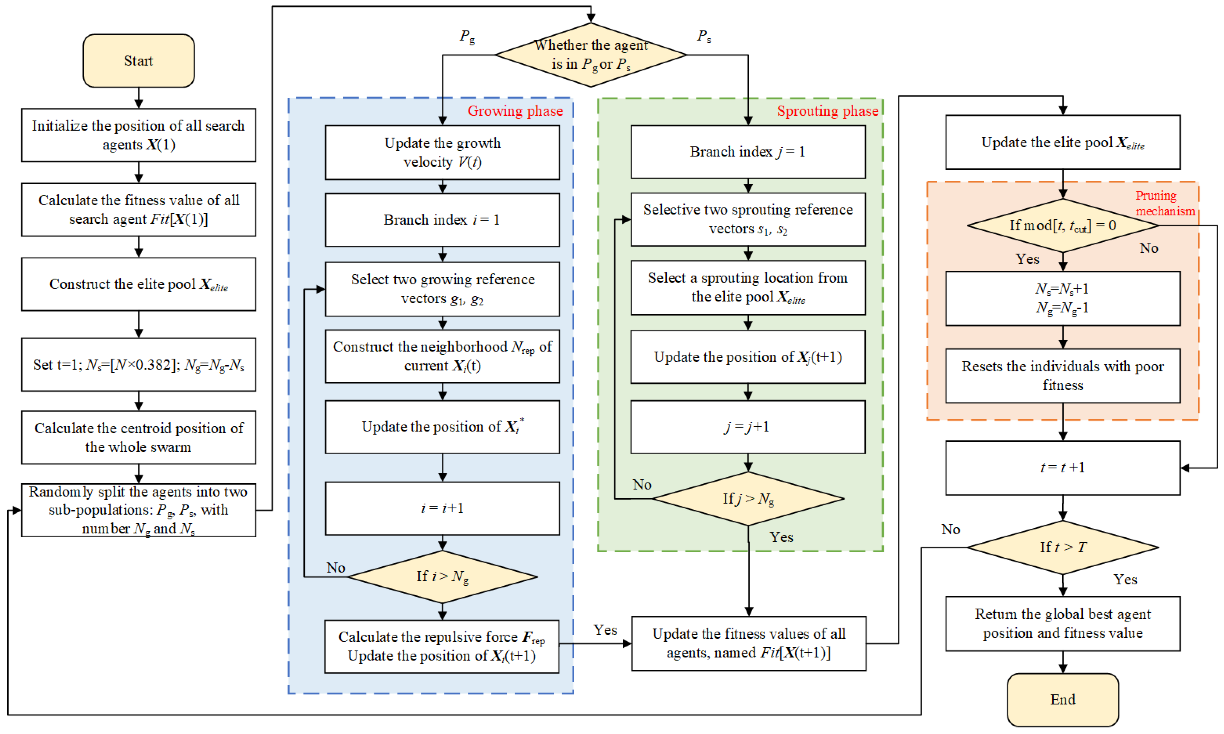
4.1.3. The Swarm Behavior of the Growing Stage and Sprouting Stage in CGO

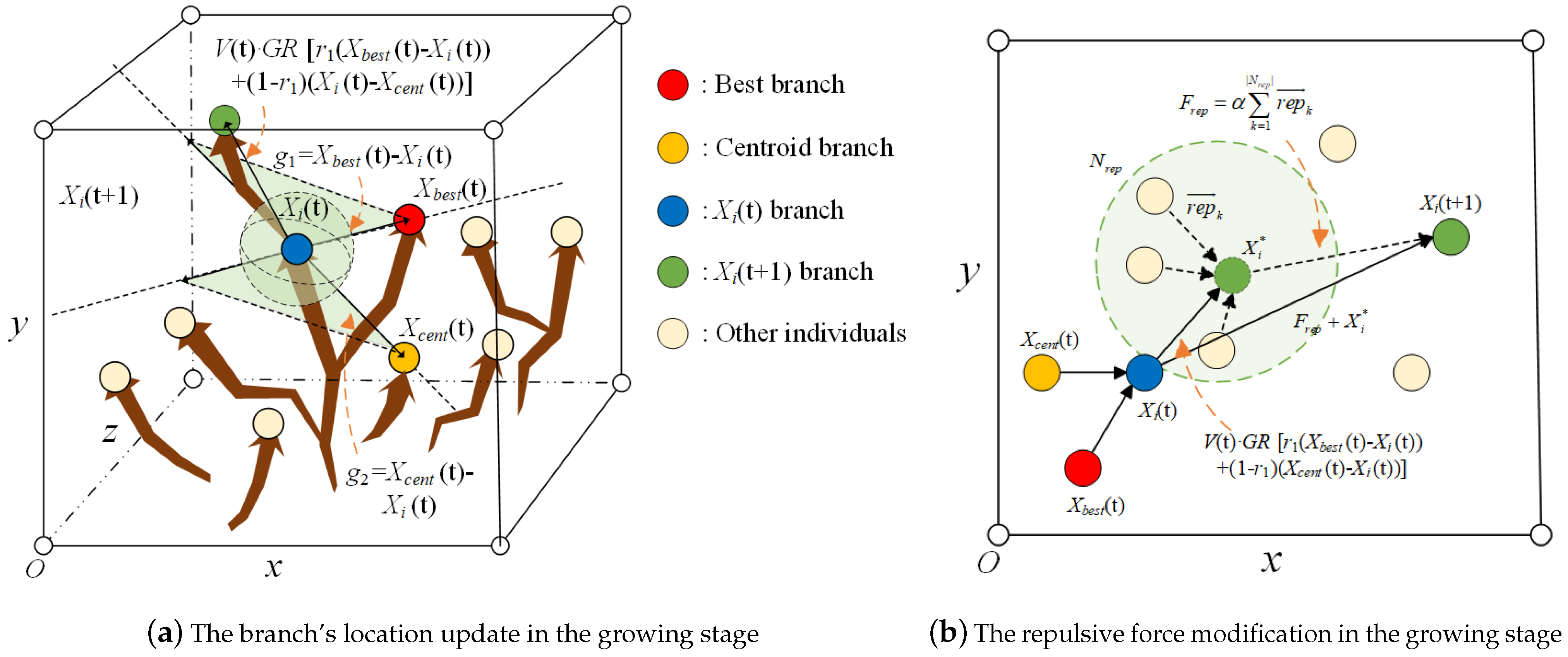
This part shows in detail how the growing stage and sprouting stage change over several iterations to better reveal how CGO works. Figure 8a shows the growth process of the clustered population (green) in three-time steps (yellow, orange, red). It can be seen that, during the exploitation stage, individuals will grow in the opposite direction of the centroid, which gives the group the possibility to explore the potential optimal solution. The swarm diversity (calculated using Equation (16)) in these four-time steps is $\{1.0318,2.2091,6.4355,15.6924\}$, respectively, indicating that the dispersion of the population is increasing. Figure 8b shows the change in population diversity when only growth occurs in 100 iterative steps. It can be seen that, in the early iteration stage, branches rapidly grow to the entire search space. The iteration is carried out. Due to the Gaussian distribution characteristic of the random number $GR(·)$ in Equation (8), the population is given the possibility of inward growth. Hence, the diversity change of the population reaches a balance.

Figure 8. The swarm behavior of growing stage.

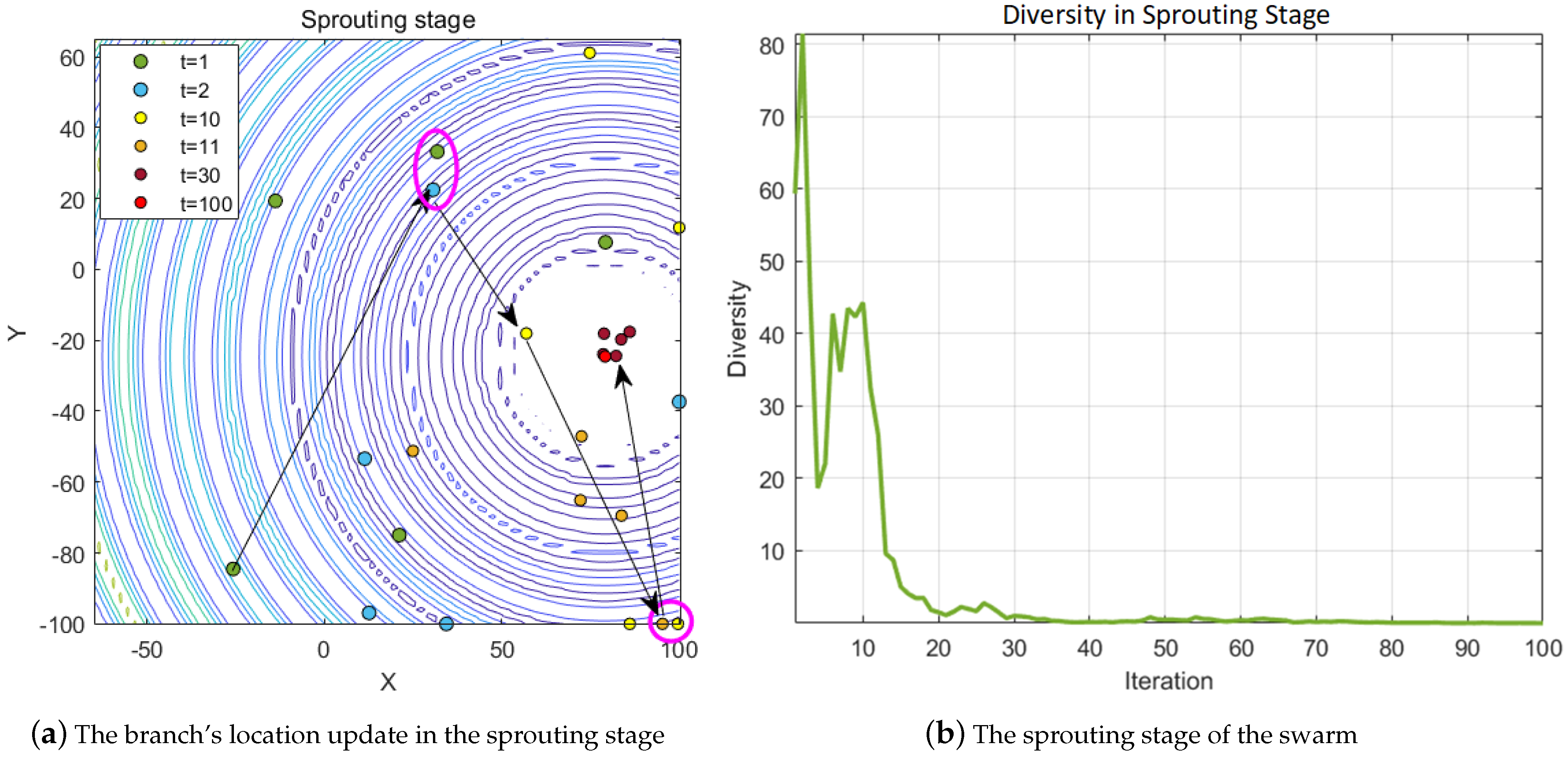
Figure 9a shows the position change of the random initial population (green) in the sprouting stage. Tracking the same particle can be seen as tracking an elite pool individual, which gives the group the ability to converge on the best individual and exploit them deeply. Figure 9b shows the change of group diversity during this process. The individual can quickly converge to an optimal location within dozens of iterations. This illustrates the exploitative power of CGO, and the exploitation process can be very rapid due to the guiding role of the elite pool.

Figure 9. The swarm behavior of sprouting stage.

4.1.4. Optimized Performance of CGO

This part computed CGO and nine other algorithms on thirty 10-dimensional, 30-dimensional, and 50-dimensional problems of CEC2017. After calculation, the solution results are shown in Table 2, Table 3 and Table 4, where the bold terms are the optimal solution results under the benchmark function in the row. We discuss the experimental results according to the class of the benchmark function.

Table 2. Results of CGO and each algorithm on CEC2017 10-dimension benchmark function.

Dim10	Metric	SMA	BKA	DBO	MVO	HHO	GWO	WOA	EWOA	AVOA	CGO
F1	mean	8266.68	4739.053	2,730,480	5526.672	260,099.9	12,115,651	159,886	1878.278	3648.82	909.6397
	std	4994.14	4575.797	12,100,971	4449.135	130,855.1	49,130,866	257,989.9	2256.088	3555.949	1312.657
F2	mean	200.0004	203.4292	4169.617	239.4137	418.6318	2083,077	6526.694	200.0001	200.0002	200
	std	0.000244	14.61524	9347.372	50.4729	612.9162	8,870,439	8233.886	6.25 $\times {10}^{-5}$	7.74 $\times {10}^{-5}$	0.000556
F3	mean	300.0005	300.0394	300.0066	300.0105	300.832	1032.75	510.9382	300	300	300
	std	0.000356	0.040747	0.029737	0.006943	0.360434	1211.673	216.0253	5.05 $\times {10}^{-14}$	2.97 $\times {10}^{-11}$	0.05145
F4	mean	418.1226	400.2291	417.4178	402.7115	404.5922	410.82	429.8399	404.5777	410.8357	402.8124
	std	27.02717	0.368128	37.60132	1.065677	2.939503	16.10206	39.54126	14.65347	19.87503	2.031058
F5	mean	514.587	523.1837	525.8744	512.3619	536.3027	509.9124	543.79	520.1479	532.3157	505.8702
	std	5.535877	10.82914	11.94835	4.332125	10.89522	4.147471	24.10335	6.914956	11.43843	3.670722
F6	mean	600.0569	613.2113	602.0653	600.3401	625.0736	600.2764	627.1772	600.191	607.7833	600
	std	0.026473	6.207428	2.852161	0.545088	8.623233	0.505634	14.27001	0.413789	6.874916	0.376712
F7	mean	721.1106	737.097	727.8944	725.8924	782.9368	724.9991	781.0224	736.7901	758.9543	717.5504
	std	3.90243	8.061024	10.25639	9.794684	20.42017	9.104373	18.51136	10.73145	18.01717	3.091354
F8	mean	814.0083	816.1218	823.0227	814.8358	829.6568	811.411	840.6548	818.4565	828.8537	808.9546
	std	6.910057	7.134712	9.804645	5.87553	5.677978	4.191306	18.43497	6.28001	9.6248	4.041537
F9	mean	900.0006	996.9719	900.715	900.0737	1291.341	901.0555	1386.16	901.786	1044.526	900
	std	0.000248	76.97673	1.178	0.222166	252.9147	1.836854	377.1481	3.667589	152.2827	0.028311
F10	mean	1634.18	1646.393	1731.504	1558.041	2084.86	1528.898	2026.746	1635.007	1774.973	1338.091
	std	217.0402	171.708	278.0634	265.2521	355.2173	236.4776	288.5847	214.847	274.8445	196.0357
F11	mean	1109.589	1119.724	1177.422	1112.028	1139.348	1115.949	1191.363	1112.144	1125.33	1110.99
	std	5.583541	14.00672	93.59059	7.123443	22.7779	10.98825	77.74997	9.057852	12.70386	9.731681
F12	mean	40,815.29	4677.256	1,198,192	184,990.1	666,948.9	345,046.9	4118,677	14,256.83	113,891	8223.305
	std	22103.3	2661.389	2,411,781	157,677.4	588,860.3	602,592.4	4,532,162	14,667.9	159,196.4	4117.475
F13	mean	9944.627	1708.386	8170.538	9950.984	15,744.89	9069.675	14,967.97	11,504.91	10,669.88	6962.14
	std	12,150.08	219.6747	8328.704	10,701.32	10,984.25	4342.81	11,770.13	7273.426	10,316.41	2133.539
F14	mean	1432.842	1461.327	1469.364	1429.206	1506.33	2804.283	1719.29	1450.349	1547.135	2542.738
	std	12.83235	28.52926	45.93435	6.383776	24.13553	1788.29	810.5586	37.8395	153.6675	1008.174
F15	mean	1535.643	1568.847	3777.796	1524.963	1874.566	3007.193	2981.174	1518.939	2655.781	2120.204
	std	40.2689	45.88032	6889.98	16.95419	285.0992	1745.55	1675.847	11.87116	1221.481	547.3905
F16	mean	1666.114	1668.652	1707.159	1734.628	1886.368	1731.093	1803.73	1683.151	1735.729	1605.374
	std	74.81463	64.8423	92.6201	124.6254	154.7654	126.6304	103.9091	85.00248	100.181	85.03682
F17	mean	1743.335	1742.301	1739.092	1776.298	1770.174	1745.333	1780.843	1741.61	1762.141	1719.197
	std	33.47695	15.22163	24.4916	59.94609	32.92266	28.44315	34.96231	37.90769	36.61525	37.18651
F18	mean	31,255.52	1940.021	16,686.22	15,806.82	15,938.03	27,407.55	22,899.76	4475.137	18,418.8	15,017.9
	std	15,015.99	91.45734	13,836.75	10,797.9	10,894.6	12,827.75	10,053.85	3535.98	13,621.85	10,590.26
F19	mean	2540.252	1946.878	5288.085	1911.594	5556.47	5072.625	22,607.98	2016.213	6279.039	2412.285
	std	2390.425	35.70505	9458.332	3.276767	5577.489	4856.778	18,445.95	155.5032	4728.916	693.1796
F20	mean	2019.561	2044.232	2036.46	2057.376	2122.354	2054.632	2151.184	2027.061	2063.023	2023.319
	std	8.705578	17.73782	31.07756	54.71106	60.23838	40.99333	65.72369	17.83318	41.52972	8.311478
F21	mean	2303.541	2207.166	2231.629	2275.52	2310.186	2305.646	2287.461	2200.699	2229.067	2266.624
	std	43.84289	24.59015	50.46098	56.74481	56.42607	25.03461	65.64223	1.305238	55.58011	57.47365
F22	mean	2302.104	2296.03	2303.841	2300.079	2310.878	2305.814	2310.654	2296.342	2303.041	2300.611
	std	0.799772	21.80677	3.080084	17.67155	15.96531	6.797469	21.82669	18.56814	17.34343	0.386774
F23	mean	2619.018	2618.165	2630.715	2615.202	2659.144	2614.549	2648.68	2625.479	2632.996	2611.601
	std	6.436286	9.354392	10.43581	9.509349	22.87696	8.735884	22.02415	10.55476	14.50273	4.589338
F24	mean	2755.21	2736.46	2707.923	2695.748	2774.438	2719.56	2765.795	2591.561	2747.128	2731.876
	std	8.751149	56.80963	103.1558	100.4832	98.02254	70.44743	65.20339	121.7098	86.04227	13.06646
F25	mean	2924.353	2926.255	2934.062	2907.575	2932.397	2937.132	2946.253	2926.572	2929.308	2921.637
	std	27.10241	32.52168	26.56042	19.14334	43.29856	14.72147	19.25461	25.88307	25.29819	23.62066
F26	mean	2954.321	2948.182	3018.523	2900.081	3378.372	2981.266	3235.984	2898.325	3068.938	2860
	std	32.03815	125.0412	73.5701	0.016775	452.4665	208.603	472.5794	36.49603	275.9875	96.60918
F27	mean	3090.32	3094.747	3102.175	3097.007	3150.962	3093.93	3131.422	3102.24	3098.998	3092.865
	std	0.938866	8.33059	15.55479	20.07032	42.94666	5.153881	35.20242	17.03681	8.860838	2.232284
F28	mean	3184.214	3278.26	3249.147	3242.572	3310.669	3355.78	3272.393	3215.868	3284.408	3322.626
	std	122.8897	180.961	148.987	180.4213	156.6027	93.39403	107.6636	134.6152	130.4064	126.0767
F29	mean	3174.896	3182.079	3207.121	3185.565	3311.76	3180.459	3323.452	3206.878	3235.547	3159.756
	std	41.2028	32.90197	59.12622	62.16986	108.2832	52.18576	93.80797	45.77878	52.87686	22.40437
F30	mean	48,147.09	293,301.7	631,677.1	408,604.1	737,280	590,766	377,696.8	274,603.5	98,507.87	193,485.8
	std	181,844.3	464,942.7	506,220.3	561,209.6	850,133.8	810,102	470,485.7	418,395.6	251,096.9	379,787.2
Friedman	ranking	3.9	4.233333	6.3	4.166667	8.5	6.066667	8.933333	3.7	6.5	2.5333

The bold terms are the best solution results under the benchmark function in the row.

Table 3. Results of CGO and each algorithm on CEC2017 30-dimension benchmark function.

Dim30	Metric	SMA	BKA	DBO	MVO	HHO	GWO	WOA	EWOA	AVOA	CGO
F1	mean	5377.25	4.36 $\times {10}^8$	3,853,111	148,587.7	12,613,239	1.01E+09	73,686,823	4803.645	5200.88	11,300
	std	6570.627	6.82 $\times {10}^8$	7,561,119	36,216.71	3,034,137	9.72 $\times {10}^8$	50,454,412	3485.719	4824.25	249,898
F2	mean	3.47 $\times {10}^9$	1.3 $\times {10}^{22}$	2.41 $\times {10}^{29}$	6.27 $\times {10}^{10}$	1.87 $\times {10}^{17}$	1.5 $\times {10}^{28}$	1.15 $\times {10}^{28}$	6.3 $\times {10}^{10}$	5.91 $\times {10}^{11}$	368,316
	std	1.43 $\times {10}^{10}$	5.81 $\times {10}^{22}$	1.08 $\times {10}^{30}$	1.74 $\times {10}^{11}$	4.41 × 1017	5.41 $\times {10}^{28}$	5.12 $\times {10}^{28}$	1.44 $\times {10}^{11}$	1.36 $\times {10}^{12}$	8.97 $\times {10}^{13}$
F3	mean	319.4433	4898.249	59,378.75	309.528	12,424.32	34,175.9	231,964.3	22,734.7	6124.844	6238.848
	std	18.60516	2764.831	21,400.9	4.355009	2451.681	9293.068	60,932.77	6121.409	3018.501	5286.609
F4	mean	492.5348	508.5619	526.8319	490.7313	526.6213	548.6142	591.6376	490.0949	497.5229	478.4643
	std	7.808333	33.57862	29.63409	7.440504	42.79235	36.22844	47.64591	17.82984	21.87513	29.7184
F5	mean	604.449	700.1549	677.9418	589.9032	737.0991	590.5285	792.6595	650.4369	705.993	581.8796
	std	27.33692	36.96952	44.57322	17.28071	27.72857	19.68565	70.1286	39.49253	45.15956	23.11887
F6	mean	601.7082	652.4253	625.5884	613.5183	660.4253	605.0337	667.7606	616.4232	641.1062	601.9366
	std	0.68367	7.042487	8.201668	8.590965	6.792604	1.738516	8.863137	8.805272	9.224886	5.243016
F7	mean	826.3549	1136.444	924.626	847.5887	1241.857	839.5995	1215.028	911.1909	1123.163	772.7977
	std	19.67014	54.90433	87.47363	23.20406	64.54117	34.53351	70.30625	45.99091	87.02117	10.72138
F8	mean	890.7417	954.7519	983.5396	897.947	958.2976	870.9667	1009.694	932.3289	958.1829	872.1521
	std	28.47621	22.19789	45.33455	24.02805	20.98769	19.38737	39.38077	32.4189	29.65787	19.30533
F9	mean	2998.866	4394.904	4815.675	2751.874	7043.877	1510.893	7922.927	3057.889	4989.181	901.1183
	std	1769.735	529.1601	2046.505	2234.605	626.1384	408.6233	3329.587	999.9277	735.8032	8.957735
F10	mean	4301.491	4707.436	5226.517	4302.91	5529.892	4345.095	6397.458	4689.725	5483.455	3394.958
	std	720.7308	490.3054	862.3125	628.635	595.7265	1146.752	606.9268	697.3967	649.8394	451.398
F11	mean	1237.795	1294.034	1462.895	1323.825	1257.058	1590.672	2463.961	1213.476	1241.468	1173.995
	std	53.72564	64.36796	125.3477	64.88334	34.03296	562.5162	946.9763	31.50631	44.10681	24.58917
F12	mean	2,778,663	5,766,594	25,790,212	8,607,554	10,984,077	36,057,553	1.18 $\times {10}^8$	176,433	2,509,225	614,565
	std	1,234,357	3,553,901	37,002,731	6,609,923	7,757,406	35,120,203	55,559,817	80,536.63	2,278,251	799,146.2
F13	mean	38,098.18	105,459.5	4,309,217	149,825.8	333,449.8	19,852,758	222,865.7	15,230.66	57,366.99	15,203.03
	std	25,643.7	85,414	9,169,298	114,524	166,746.9	77,341,414	141,262.6	15,925.65	27,808.29	12,944.46
F14	mean	62,781.13	3426.036	52,106.33	11,873.6	98,680.75	169,391.2	800,536.3	29,645.99	49,452.25	8200.661
	std	44,319.46	7756.405	64,522.26	7631.825	102,060.8	271,020.1	878,213.7	23,803.54	54,028.89	21,559.78
F15	mean	29,344.42	13,734.66	91,986.99	63,872.16	58,002.99	255,257.6	101,402.8	9565.829	28,754.01	4382.162
	std	13,411.52	6775.954	91,069.94	37,859.12	35,084.53	557,425.7	58,070.03	8020.26	15,532.17	1422.259
F16	mean	2452.354	2678.542	2829.228	2402.265	3025.788	2381.102	3746.378	2732.442	2984.377	2343.871
	std	328.0747	276.737	362.5582	272.9544	351.328	281.557	460.0131	247.8367	299.5409	298.8409
F17	mean	2130.374	2155.697	2440.673	2017.628	2558.058	1948.542	2620.225	2212.632	2346.537	1962.032
	std	213.7428	216.4221	191.0118	136.448	237.0936	122.3204	284.0307	169.861	276.5934	175.0651
F18	mean	617,766	47,971.07	1,338,814	207,722	1,210,834	864,938.1	5,645,910	226,536.3	696,127.5	101,352.9
	std	503,903.6	27,499.95	2,621,422	118,851.8	1,280,763	943,209.7	4,247,208	211,816.6	476,743.9	84,960.42
F19	mean	28,885.12	23,485.62	403,727.1	777,344.4	332,815.2	207,7561	6,557,646	8966.789	17,006.41	5016.343
	std	20,718.82	18,747.19	766,456.2	624,438.3	200,943.1	6,559,131	5,780,143	8030.889	15,618.75	1513.306
F20	mean	2470.818	2444.716	2635.959	2471.466	2670.439	2315.197	2836.165	2494.282	2645.821	2218.891
	std	215.0865	109.7244	194.7875	166.0301	227.8806	126.5749	209.7384	182.0839	203.3636	109.6985
F21	mean	2410.606	2495.258	2499.837	2388.566	2537.944	2372.215	2560.471	2417.544	2492.849	2353.343
	std	28.96407	28.68166	52.74283	18.30179	43.87005	15.75393	53.468	30.46358	54.43004	7.248308
F22	mean	5317.714	5197.949	4758.352	3573.863	5804.97	4419.696	6243.803	3210.544	5493.735	2306.643
	std	1467.211	1786.655	1913.324	1655.995	2285.188	1870.104	2333.746	1643.107	2453.88	1183.754
F23	mean	2750.156	2986.681	2879.68	2751.444	3082.055	2758.081	3032.201	2784.794	2939.198	2693.781
	std	28.63822	82.93639	44.89913	21.55668	100.8779	56.95738	93.98266	35.37427	102.1256	17.79106
F24	mean	2926.488	3111.664	3036.058	2898.594	3364.776	2918.996	3204.151	2946.532	3098.205	2861.949
	std	26.40902	91.40193	65.36192	27.61287	113.5284	54.54668	87.78498	32.83874	79.7649	9.676014
F25	mean	2887.425	2937.897	2923.9	2888.498	2916.546	2959.329	2986.076	2896.932	2907.936	2920.704
	std	1.27469	33.69789	24.45055	6.24729	17.88146	44.50676	26.19608	19.13206	20.11236	23.39826
F26	mean	4793.489	6782.387	6062.839	4411.46	6910.814	4456.224	7639.578	5262.013	6236.18	3750.938
	std	385.7911	1384.81	819.6153	413.4554	1334.103	294.7987	1054.782	904.5974	1459.199	881.4943
F27	mean	3217.702	3315.1	3254.219	3220.262	3337.356	3231.987	3379.591	3237.475	3270.777	3219.856
	std	11.63925	72.51759	18.37827	12.53776	62.72374	10.81272	67.17871	29.86115	34.92116	11.68746
F28	mean	3237.184	3275.876	3330.811	3242.101	3280.472	3364.404	3359.567	3225.669	3220.66	3206.159
	std	22.44636	42.02447	67.59715	34.80588	12.64479	59.90671	42.4757	38.67191	16.42594	17.06787
F29	mean	3811.943	4246.346	4169.491	3738.022	4395.124	3748.175	4996.02	3842.763	4213.6	3579.192
	std	147.6799	254.7624	220.7401	128.9396	345.528	190.1221	422.5032	255.025	350.5144	136.1354
F30	mean	19,731.11	673,527.9	1,128,029	2,617,755	1,793,350	7,804,491	21,177,561	9601.592	94,281.38	9421.892
	std	6175.026	552,366.1	1,516,103	1,370,942	1,038,325	6,531,364	21,178,595	3529.088	69,595.69	5107.745
Friedman	ranking	3.5	5.866667	7.166667	3.866667	7.966667	5.7	9.6	3.966667	5.733333	1.633333

The bold terms are the best solution results under the benchmark function in the row.

Table 4. Results of CGO and each algorithm on CEC2017 50-dimension benchmark function.

Dim10	Metric	SMA	BKA	DBO	MVO	HHO	GWO	WOA	EWOA	AVOA	CGO
F1	mean	60,715.58	6.19 $\times {10}^9$	1.55 $\times {10}^8$	1,423,875	76,313,354	4.71 $\times {10}^9$	6.06 $\times {10}^8$	4201.759	6876.674	440,031.7
	std	21,273.6	4.5 $\times {10}^9$	1.17 $\times {10}^8$	246,778.2	11,912,630	2.27 $\times {10}^9$	2.56 $\times {10}^8$	4783.103	6592.133	3342.474
F2	mean	7.83 $\times {10}^{24}$	4.48 $\times {10}^{43}$	2.66 $\times {10}^{59}$	6.83 $\times {10}^{23}$	2.54 $\times {10}^{44}$	2.64 $\times {10}^{50}$	5.14 $\times {10}^{65}$	1.04 $\times {10}^{30}$	2.26 $\times {10}^{27}$	2.48 $\times {10}^{18}$
	std	3.5 $\times {10}^{25}$	9.68 $\times {10}^{43}$	1.16 $\times {10}^{60}$	1.55 $\times {10}^{24}$	1.1 $\times {10}^{25}$	8.31 $\times {10}^{50}$	2.27 $\times {10}^{66}$	4.4 $\times {10}^{30}$	6.83 $\times {10}^{27}$	1.28 $\times {10}^{32}$
F3	mean	4521.647	21,979.67	228,063.7	1409.196	55289.21	88,639.31	168,728.8	104,801.7	58,462.22	60,065.37
	std	1794.405	5372.987	49,887.45	297.0551	12,257.11	11,963.71	47,580.64	23,139.97	13,891.36	23,000
F4	mean	576.9389	949.9207	805.75	563.2629	712.4008	891.8574	1030.664	515.0034	567.9258	519.6674
	std	32.05013	307.121	247.0451	42.06515	70.7315	136.898	128.4592	49.43537	52.3251	44.94962
F5	mean	709.1999	863.8638	953.4783	707.6505	884.7758	698.5931	955.3329	800.2986	847.3773	715.3925
	std	37.28214	38.88459	93.91457	34.11924	33.75688	70.29152	71.52801	70.56504	37.31424	19.22539
F6	mean	613.947	661.9436	648.0411	629.4978	673.3391	612.955	683.6265	634.0399	647.9081	609.8787
	std	7.649736	4.126708	10.12797	11.30414	5.176703	4.541637	9.16058	11.42608	7.823594	0.457
F7	mean	995.1085	1583.875	1159.888	1002.98	1785.507	1024.605	1740.582	1703.778	1514.404	839.422
	std	49.38504	69.66849	136.8953	53.22727	81.79833	58.98407	117.9619	120.5737	91.05087	75.66296
F8	mean	1019.689	1146.7	1223.757	997.9437	1181.799	1006.082	1268.272	1101.415	1151.118	1017.22
	std	47.53974	33.58786	88.23056	48.87687	25.94531	31.50603	74.84276	45.74084	62.82611	25.88947
F9	mean	11,285.98	13,715.37	16,576.95	13,981.29	23,487.35	7488.56	26,733.21	9861.731	12,909.87	1230.147
	std	2753.415	1164.746	5415.422	9078.104	3516.278	4480.532	7394.689	2935.511	1597.679	71
F10	mean	7147.145	8160.722	9364.417	6914.081	9003.113	7452.659	10,826.2	7608.95	8090.378	5389.16
	std	896.7854	831.2271	1147.531	704.9839	945.015	2031.746	1260.341	999.3778	811.2726	794.8772
F11	mean	1343.204	1662.605	2009.743	1470.06	1521.001	3361.828	2297.495	1332.374	1327.386	1262.033
	std	72.79716	265.8163	380.2538	82.58486	94.79113	1549.037	208.9122	48.87874	61.43538	105.9204
F12	mean	12,613,598	77,774,045	2.24 $\times {10}^8$	54,019,523	86,223,822	2.89 $\times {10}^8$	5.62 $\times {10}^8$	2,457,199	13,802,842	5,927,494
	std	6,324,084	1.15 $\times {10}^8$	2.63 $\times {10}^8$	29,881,484	47,319,180	2.98 $\times {10}^8$	2.87 $\times {10}^8$	1,502,630	6,891,542	1,791,801
F13	mean	42,480.47	1,388,322	9,526,966	185,928.9	2,480,812	1.33 $\times {10}^8$	7,959,201	9581.048	86,155.39	8253.086
	std	9436.686	2,989,116	11,614,064	100,051.8	1,650,954	1.2 $\times {10}^8$	8,311,562	8363.528	55,472.56	6486.681
F14	mean	299,607.9	19,124.7	982,315.2	104,037.7	763,382	947,260.2	1,808,266	106,417	287,420.3	49,935.36
	std	154,164.6	26,630.75	109,1507	93,808.35	499,233.7	998,844.4	1,504,569	81,496.26	156,134.7	56,338.87
F15	mean	24,460.28	60,828.63	720,617.2	98,359.37	458,727.8	4,521,998	825,800	7615.579	45,620.46	13,639.9
	std	10,860.6	46,892.59	2,585,498	59,608.07	183,021	15,978,067	1,648,218	6523.728	17,928.28	5248.987
F16	mean	3317.854	3624.933	4259.147	3105.153	4779.948	3143.2	5326.331	3245.916	3887.755	2775.846
	std	399.8752	454.4592	709.0213	389.9807	712.4875	546.5186	876.6649	401.7988	369.6291	400.5497
F17	mean	3166.359	3110.281	4067.17	3050.249	3689.603	2873.124	4066.177	3038.626	3528.014	2874.947
	std	338.6763	252.3009	413.9516	295.5947	321.8392	497.1003	545.2768	405.8827	386.374	320.2662
F18	mean	2,176,417	319,607.7	6,555,171	1,263,269	5,844,859	3,935,318	13,116,738	676,520.5	1,814,154	493,333.4
	std	1,116,703	221,443.8	9,386,293	877,055.7	4,162,457	3,931,363	8,841,144	563,721.4	1,594,325	1,106,656
F19	mean	16,295.18	536,067.7	254,7785	4,209,524	993,633.6	3,150,647	4,860,970	12,104.67	27,508.86	16,543.29
	std	16,280.52	676,035.1	5,107,564	2,601,440	507,672.3	3,679,501	4,553,916	11,980.4	17,573.31	7524.625
F20	mean	3105.9	3019.668	3443.12	3068.48	3537.831	2901.1	3,727	3100.009	3493.748	2631.8
	std	241.7975	216.8104	337.3048	335.3027	294.5325	299.7464	340.0154	351.5468	369.5631	265.2259
F21	mean	2525.959	2721.131	2744.463	2497.833	2850.096	2495.973	2961.023	2568.34	2722.453	2465.665
	std	46.62297	65.63287	83.30057	49.88781	90.46669	25.41674	86.71692	53.72395	70.00154	19.36694
F22	mean	9029.491	9842.286	10,611.63	8505.021	11,258.47	9089.939	12,279.66	9225.202	10,036.17	6994.803
	std	1039.094	695.9278	1343.249	862.7647	863.9258	964.6762	1551.255	991.3282	936.2804	968.9891
F23	mean	2965.571	3512.163	3283.981	2921.341	3721.473	2936.685	3684.548	3061.859	3333.714	2931.938
	std	47.53908	143.57	110.9179	38.99199	153.8934	42.68835	164.2876	82.13251	134.9634	30.98419
F24	mean	3128.738	3648.623	3373.164	3062.255	4002.264	3082.233	3699.773	3248.505	3553.721	3090.03
	std	51.5166	132.9464	86.99671	46.96662	167.5729	40.90279	163.9739	73.93475	91.98767	21.85485
F25	mean	3050.238	3458.081	3204.67	3039.676	3188.152	3442.478	3382.083	3052.538	3100.415	3077.409
	std	37.41275	161.9894	131.5427	29.03659	38.73183	167.2651	103.6927	34.174	24.67113	22.7515
F26	mean	5366.73	10,471.81	9842.868	5951.706	10,884.81	6079.835	13,043.28	6946.212	9670.933	8098.113
	std	1317.369	2811.786	1274.646	392.3547	1074.937	823.4894	1482.289	726.3159	1934.586	222
F27	mean	3394.057	3975.346	3621.03	3351.096	4140.814	3524.827	4351.426	3508.179	3737.223	3432.68
	std	71.6175	252.2562	127.594	59.3161	219.5832	72.02516	433.7488	136.1074	158.4083	63.80357
F28	mean	3318.263	3904.922	5162.091	3286.958	3489.387	3935.572	4026.631	3306.993	3350.13	3355.777
	std	27.92524	278.72	2418.651	25.4033	73.30007	236.1407	293.2987	21.61349	38.43438	22.29936
F29	mean	4315.925	5867.801	5327.154	4,565	5853.151	4405.615	7572.446	4612.183	5019.832	4103.622
	std	428.7486	569.1849	415.6254	431.6857	465.5058	235.6915	949.6659	363.3273	373.5984	219.1384
F30	mean	2,049,840	19,628,600	23,184,652	57,211,506	30,463,801	99,569,806	1.74 $\times {10}^8$	1,087,281	4,168,414	1,080,447
	std	635,292.4	6,331,935	19,630,612	18,410,263	7,700,490	28,094,962	53,107,108	322,302.3	1,272,446	169,457
Friedman	ranking	3.466667	6.333333	7.8	3.366667	7.733333	5.433333	9.533333	3.7	5.4	2.233333

The bold terms are the best solution results under the benchmark function in the row.

1. Unimodal functions (F1–F3): These three functions only have one global best solution. The gradient near the optimal value of those functions is very small relative to other spaces, which is suitable for testing the algorithm’s exploitation ability. CGO performs better than other algorithms on the 10-dimensional F1–F3 problem. This shows that CGO has enough exploitation ability near the optimal value. Because the sprouting stage of CGO is guided by the elite pool, CGO can concentrate on exploitation in such unimodal problems. Compared with other swarm algorithms, such as BKA, DBO, EWOA, etc., a part of swarms are allocated to the exploration in the middle and later iterations, so the results of the CGO algorithm are better.

2. Simple multimodal functions (F4–F10): These functions have many locally optimal solutions suitable for testing the algorithm’s exploration ability. CGO exhibits the best global exploration capabilities and gets the best results on all benchmark functions except the 30-dimensional F4 function. The highly dispersed and repulsive mechanism of the growth stage of CGO can improve the diversity of the population, so it is conducive to finding more potential optimal solutions.

3. Hybrid functions (F11–F20): This kind of function contains many unimodal and multimodal functions, which are more challenging to optimize. CGO achieved the best results in 20 out of 30 benchmark functions in 10, 30, and 50 dimensions. In addition, EWOA and BKA are also prominent in this kind of function. The pooling mechanism and priority selection strategy of EWOA improve the local and global search capability of WOA, and BKA integrates the Cauchy mutation strategy and the leader strategy to enhance the global search capability and the convergence speed of the algorithm. This also leaves room for improvements in CGO algorithms.

4. Composition functions (F21–F30): The composition benchmark functions combine all the above function combinations. CGO achieved the best results in 17 of the 30 benchmark functions in 10, 30, and 50 dimensions. This shows that CGO’s optimization performance is better than that of the existing advanced algorithms.

The main reason why CGO outperforms other algorithms in unimodal functions, multimodal functions, and composition functions is that the algorithm introduces an elite pool. It is different from other algorithms, such as DBO, WOA, BKA, etc., which only record the position of the only optimal solution. In the process of exploration, CGO can record several optimal locations, median locations, and centroid locations of the whole world without losing the statistical characteristics of the population, so that CGO has the possibility of discovering potential local optimal solutions. The sprouting stage is completely based on the guidance of the elite pool, and the synthesis of two vectors ${\overrightarrow{s}}_1$ and ${\overrightarrow{s}}_2$ is directional and random. These mechanisms can make CGO’s ability to exploit the optimal solution of the solution space significantly better than other algorithms.

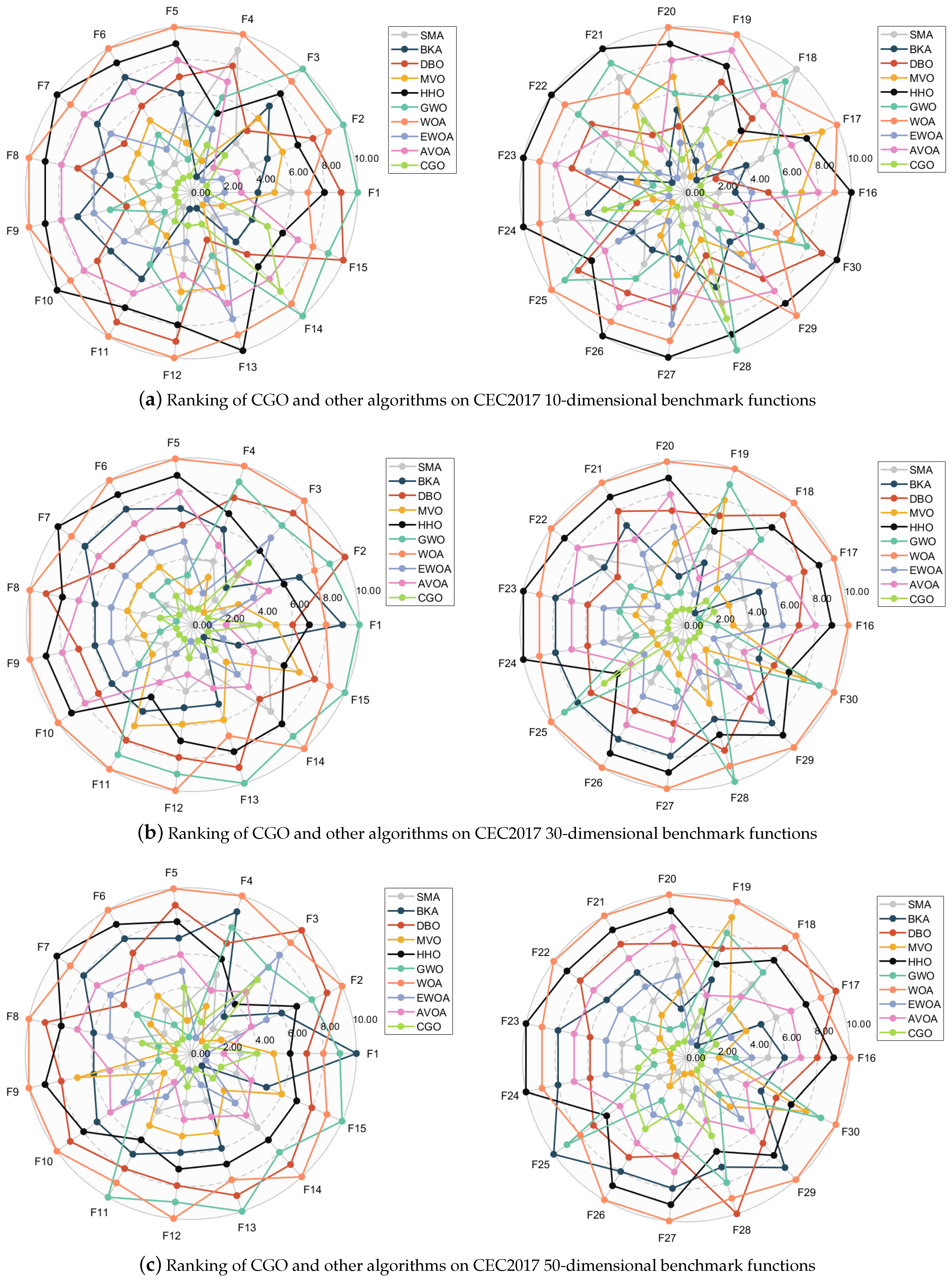
CGO and nine other algorithms’ rank on all CEC2017 benchmark functions are shown in Figure 10. The green line represents the CGO algorithm, which is distributed in the center area of the radar map, indicating that, in most problems, CGO is significantly better than other algorithms.

Figure 10. Ranking of CGO and other algorithms on CEC2017 benchmark functions.

Table 5 shows the Friedman test rankings for all the algorithms above. The proposed CGO algorithm performs very well, with a comprehensive ranking of 2.5000 on the 10-dimension functions, 2.4333 on the 30-dimension function, and 2.4000 on the 50-dimension functions. In particular, as the dimension of the solution space increases, the CGO algorithm shows better optimization performance.

Table 5. The Friedman test ranking of CGO and other algorithms on CEC2017.

Algorithm	10-Dim	30-Dim	50-Dim
SMA	3.9000	3.5000	3.4667
BKA	4.2333	5.8667	6.3333
DBO	6.3000	7.1667	7.8000
MVO	4.1667	3.8667	3.3667
HHO	8.5667	7.9667	7.7333
GWO	6.1333	5.7000	5.4333
WOA	8.9667	9.6000	9.5333
EWOA	3.7000	3.9667	3.7000
AVOA	6.5000	5.7333	5.4000
CGO	2.5333	1.6333	2.2333

Additionally, the Wilcoxon test [24] was conducted on CGO and nine other algorithms based on 10-, 30-, and 50-dimensional CEC2017 functions. As the test outcomes show in Table 6, in most cases, the attained p-values are less than 5%. Only in the case of a 10-dimensional function does the p-value of CGO vs. BKA and CGO vs. EWOA exceed 5%. This shows that CGO’s performance is close to that of BKA and EWOA in such cases. In most cases, the optimization performance of CGO is significantly better than that of other algorithms.

Table 6. The Wilcoxon test result of CGO and other algorithms on CEC2017.

Comparison	10-Dimensional Functions	30-Dimensional Functions	50-Dimensional Functions	All Functions
CGO vs. SMA	1.1748 $\times {10}^{-2}$	3.1123 $\times {10}^{-5}$	1.7988 $\times {10}^{-5}$	2.43 $\times {10}^{-11}$
CGO vs. BKA	1.5886 $\times {10}^{-1}$	8.9443 $\times {10}^{-4}$	6.1564 $\times {10}^{-4}$	2.63 $\times {10}^{-7}$
CGO vs. DBO	3.7243 $\times {10}^{-5}$	1.7344 $\times {10}^{-6}$	1.7344 $\times {10}^{-6}$	5.98 $\times {10}^{-16}$
CGO vs. MVO	2.9575 $\times {10}^{-3}$	1.7988 $\times {10}^{-5}$	2.3704 $\times {10}^{-5}$	8.48 $\times {10}^{-12}$
CGO vs. HHO	2.1266 $\times {10}^{-6}$	1.3601 $\times {10}^{-5}$	1.2381 $\times {10}^{-5}$	1.46 $\times {10}^{-14}$
CGO vs. GWO	5.7517 $\times {10}^{-6}$	1.7344 $\times {10}^{-6}$	1.7344 $\times {10}^{-6}$	2.88 $\times {10}^{-16}$
CGO vs. WOA	1.7344 $\times {10}^{-6}$	1.7344 $\times {10}^{-6}$	1.7344 $\times {10}^{-6}$	1.74 $\times {10}^{-16}$
CGO vs. EWOA	7.4438 $\times {10}^{-2}$	1.1138 $\times {10}^{-3}$	1.4936 $\times {10}^{-5}$	3.18 $\times {10}^{-9}$
CGO vs. AVOA	1.9148 $\times {10}^{-4}$	1.6394 $\times {10}^{-5}$	1.1265 $\times {10}^{-5}$	5.73 $\times {10}^{-13}$

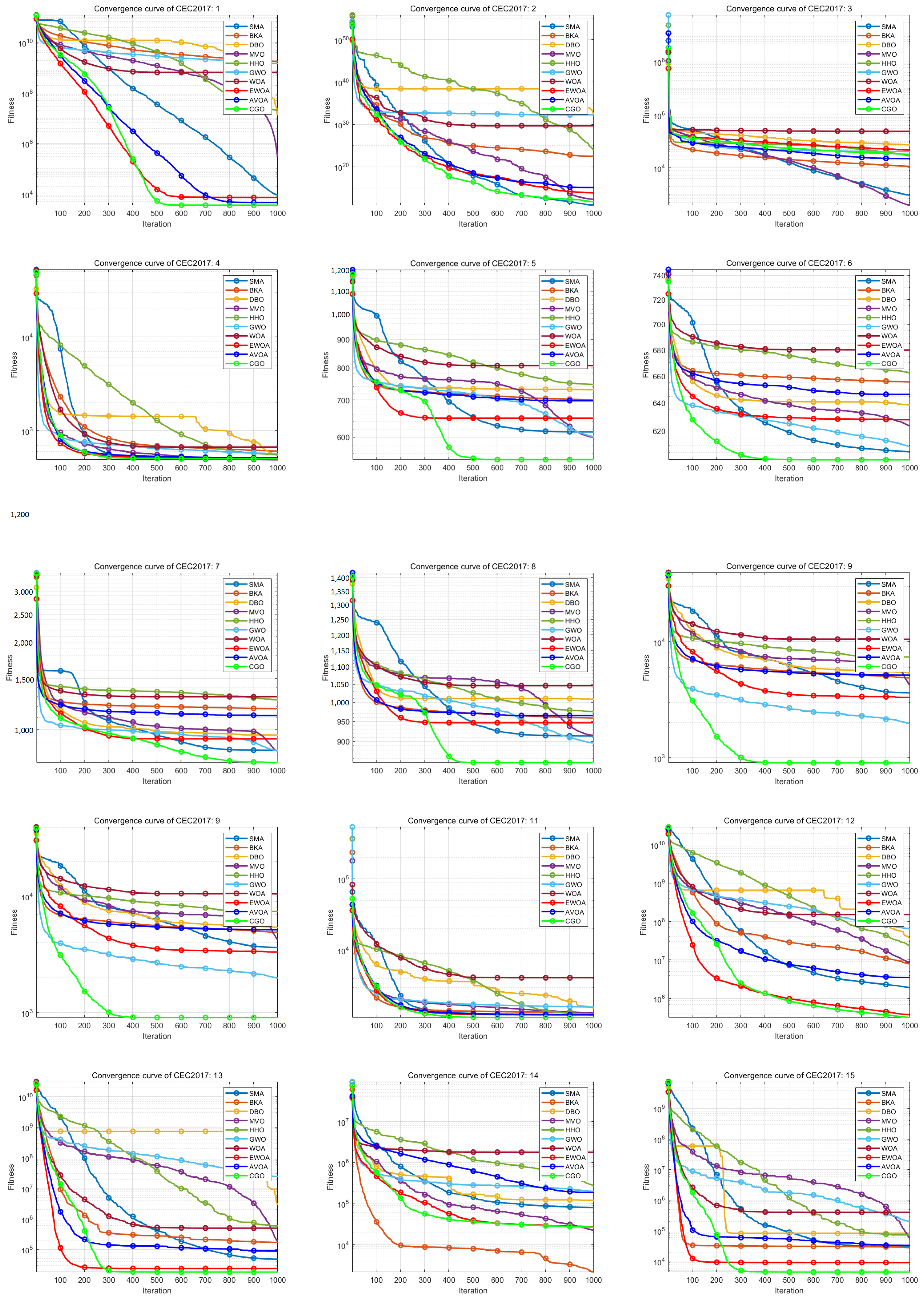
The evolution curve (Figure 11 and Figure 12) shows that CGO’s (green line) convergence speed is much faster than other algorithms, and it can quickly converge to the optimal value. CGO showed rapid evolution in the early stage of iteration, showing an excellent ability to search the global space. In contrast, in the middle and late stages of iteration, CGO maintains a persistent local exploitation ability on many functions, and its evolution curve consistently and slowly declines to avoid premature convergence.

Figure 11. Evolution curve of CGO and other algorithms on CEC2017 30-dimension reference function (F1–F15).

Figure 12. Evolution curve of CGO and other algorithms on CEC2017 30-dimension reference function (F16–F30).

4.1.5. Analysis of Pruning Mechanism in CGO

In this part, we analyzed the influence of the pruning time interval $t_{cut}$ of the pruning mechanism on the exploration and exploitation of CGO. In [25], Hussain et al. put forward an approach to measure and analyze the capability of exploitation and exploration in meta-heuristic algorithms. We used this method to measure the extent of population exploration and exploitation:

$$\begin{array}{cc}\hfill & Epl\%={\displaystyle \frac{Div}{Di{v}_{max}}}\times 100\hfill \\ \hfill & Ept\%={\displaystyle \frac{|Div-Di{v}_{max}|}{Di{v}_{max}}}\times 100\hfill \end{array}$$

(18)

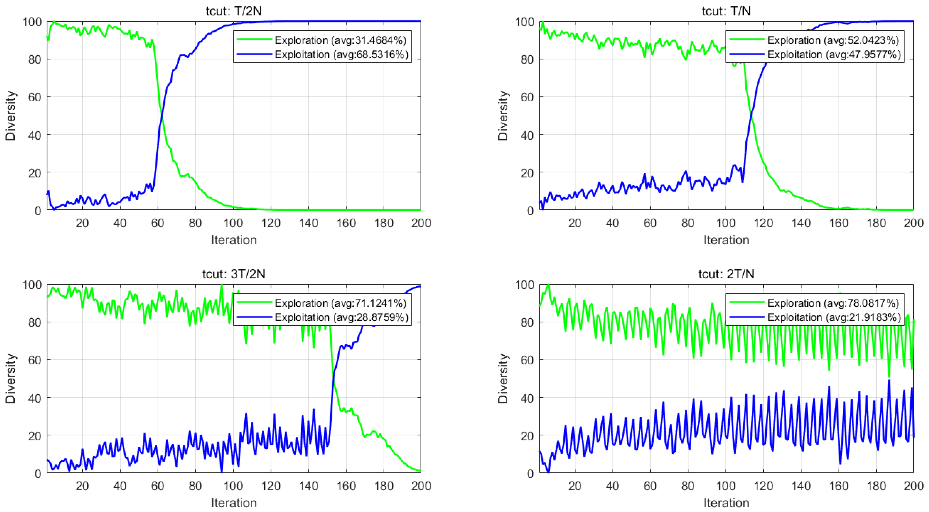
where $Di{v}_{max}$ represents the maximum diversity. $Epl\%$ and $Ept\%$ refer to the exploration percentage and exploitation percentage, respectively. Figure 13 shows the proportions of exploration (blue) and exploitation (green) capability in crown population when adjusting $t_{cut}=\{T/2N,T/N,3T/2N,2T/N\}$ on the same benchmark function CEC2017-10.

Figure 13. The influence of $t_{cut}$ on optimization.

Figure 13 shows the capability of exploitation and exploration of individuals after adjusting the pruning time interval $t_{cut}$. In Figure 13, it can be seen that there are two distinct stages of particle behavior. In the first stage, the primary behavior of the group is exploration. With the increase of $t_{cut}$, the time interval for CGO to perform pruning also increases. The duration of the exploration phase also increases, and, in this phase, particle swarms are more focused on spreading out into the search space and finding more potential locations. In each pruning period, the relative amounts of $N_g$ and $N_s$ are renewed once, and the sprouting effect gradually exceeds the growth effect. Therefore, it can be seen that the exploration capability declines with each iteration while the exploitation capability gradually increases. Until $N_g$ is reduced to 0, all individuals enter the sprouting stage, the exploration effect rapidly reduces, and the exploitation effect rapidly increases. Due to the elite guidance and randomness of the sprouting stage, Equation (12), as well as the last selection process (Section 3.5) of the pruning mechanism, the optimization does not converge immediately but continues to deepen the exploitation within the known optimal space to find a better solution.

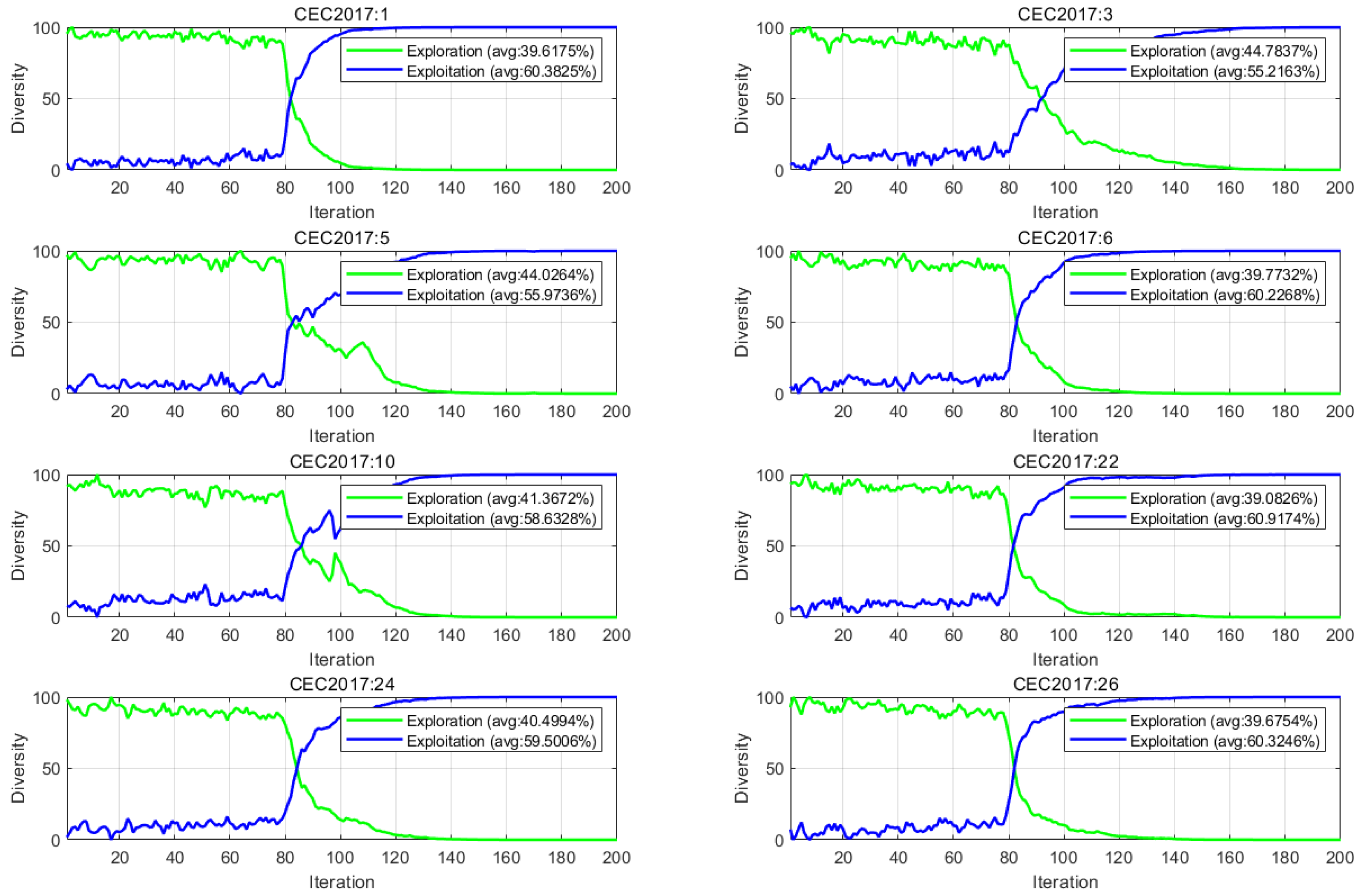
We checked the results of the diversity change of CGO at $t_{cut}=T/N$ on CEC2017 and compared the results of different $t_{cut}$ solutions. Table 7 and Figure 14 do an excellent job of explaining the ability of $t_{cut}$ to regulate exploitation and exploitation. CEC2017-1 and CEC2017-3 problems are unimodal problems, and branches do not need to explore other better solutions, so they should be more focused on exploitation. A shorter $t_{cut}$ would be more appropriate. For multimodal and hybrid problems, such as CEC2017-5, CEC2017-6, CEC2017-10, CEC2017-22, CEC2017-24, and CEC2017-26, due to the existence of a large number of locally optimal solutions, it is essential to explore the process thoroughly. Therefore, when $t_{cut}$ is more significant, the search performance is better. The more complex the problem, the more thorough the exploration phase needs to be. At the same time, when $t_{cut}=2T/N$, the CGO solution results are poor because the necessary exploitation process is lacking.

Table 7. Effects of different pruning time intervals on optimization results.

${\mathit{t}}_{\mathit{cut}}$	T/2N	T/N	3T/2N	2T/N
F1	4172.4349	5183.418	23,143	3.64 $\times {10}^8$
F3	300.09126	305.3465	761.5945	4837.87
F5	508.914549	506.915	513.1768	548.3812
F6	600.000045	600.002	600.1659	614.1876
F10	1510.25156	1404.88	1722.787	2485.58
F22	2297.31009	2291.28	2305.585	2340.852
F24	2729.52829	2727.559	2673.21	2751.753
F26	2929.77015	2937.075	2926.37	3035.957

Figure 14. Exploitation percentage and exploration percentage on CEC2017 benchmarks.

This example illustrates how the pruning mechanism can balance and utilize the two phases of exploration and exploitation, as well as provide an adaptive approach to different problem types. Usually, we set $t_{cut}=T/N$ because this is the most balanced result.

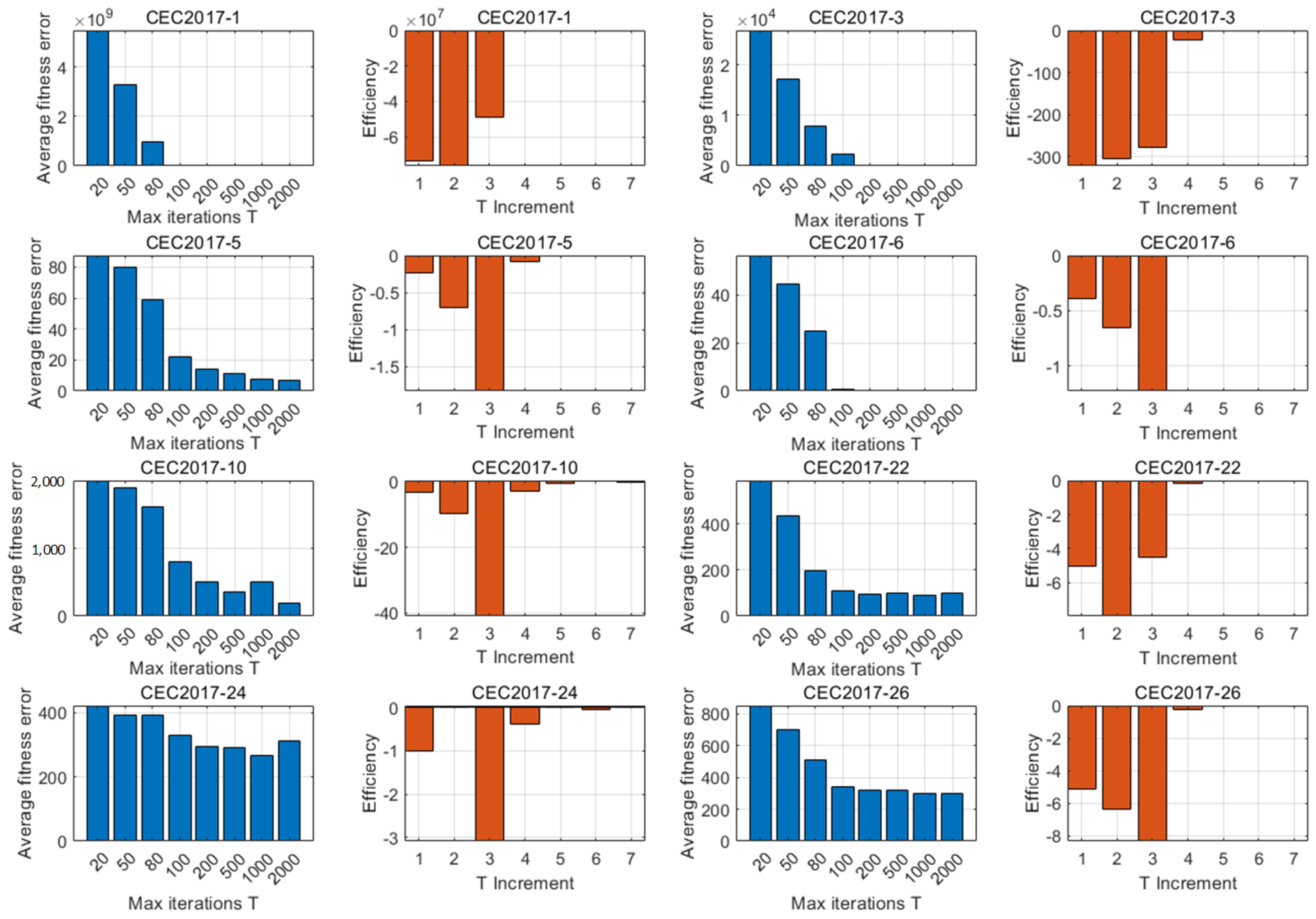
4.1.6. Influence of Population Size N and Max Iteration T on Optimization

Figure 15 and Figure 16, respectively, show the optimizing results under the number of different branches of population $N=\{10,20,50,100,150\}$ and the maximum number of iterations $T=\{20,50,80,100,200,500,1000,2000\}$. The vertical coordinate of each set of blue bars is the optimization solution error, the horizontal coordinate is the value N or T, the vertical coordinate of orange bars is the improvement efficiency, and the horizontal coordinate is the number of increases of N or T. The solution error and improvement efficiency are defined as in Equation (19).

$$\begin{array}{cc}\hfill & Error=Fi{t}^{*}\left[\mathbf{X}\left(T\right)\right]-f^{*}\hfill \\ \hfill & Efficienc{y}^N=(Erro{r}_{k+1}^N-Erro{r}_k^N)/(N_{k+1}-N_k)\hfill \\ \hfill & Efficienc{y}^T=(Erro{r}_{k+1}^T-Erro{r}_k^T)/(T_{k+1}-T_k)\hfill \end{array}$$

(19)

where $f^{*}$ is the theoretical optimal solution, $Fi{t}^{*}\left[\mathbf{X}\left(T\right)\right]$ is the optimal solution obtained by CGO, and k is the serial number of the traversal settings of N and T. When N and T are increased, CGO can get better solutions. However, with the increase of N and T, the efficiency of improving results is also limited, which also causes a waste of calculation time. By comparison, in the selected 10-dimensional problem, where N takes 100 and T takes 200, it has almost reached the maximum optimization ability. Further increases in N and T will not significantly improve CGO’s ability to exploit.

Figure 15. The influence of population size N on optimization.

Figure 16. The influence of max iteration T on optimization.

Table 8 shows the solving time of CGO and nine other algorithms on thirty 10-dimensional CEC2017s. The solution parameters are set to $N=100$ and $T=200$. Each optimizer calculates each benchmark function 20 times independently and then sums $30\times 20$ operation times to calculate the average time to solve a single problem. It can be seen that CGO is ahead of most advanced optimization algorithms in average processing time, including MVO, WOA, DBO, GWO, AVOA, BKA, SMA, etc. Among the algorithms compared, only HHO has a better computation time than CGO. This shows the high efficiency of this algorithm.

Table 8. The average solving time of CGO and nine other algorithms on thirty 10-D CEC2017 functions.

	CGO	SMA	BKA	DBO	HHO	MVO	GWO	WOA	EWOA	AVOA
time	0.11943	0.37954	0.322923	0.273771	0.025686	0.268479	0.27726	0.268479	0.436167	0.300184
rank	2	9	8	5	1	3	6	4	10	7

4.2. Testing Results on CEC2020 Real-World Constrained Problems

Unlike CEC2017, CEC2020 contains a set of engineering problems with real environmental constraints called CEC2020–RW. CEC2020–RW is highly non-convex and complex and contains several equality and inequality constraints. The penalty function method is used as the constraint processing method.

There are six types of problems in CEC2020–RW: industrial chemical processes, process synthesis and design problems, mechanical engineering problems, power system problems, and livestock feed ration optimization. Mathematical expressions for these problems can be found in paper [26]. This section used CGO and nine other algorithms to solve 20 typical problems of CEC2020–RW. The selected problem names, main parameters, and theoretical optimal values are shown in Table 9. Each algorithm was independently executed 20 times, with 1000 iterations as the termination criterion, and the number of searching agents was 100. D is the problem dimension, g is the number of equality constraints, h is the number of inequality constraints, and $f^{*}$ is the theoretical optimal value.

Table 9. Names and parameters of 20 typical problems in CEC2020-RW.

No.	Name	D	g	h	${\mathit{f}}^{*}$
Industrial Chemical Processes
RW01	Heat exchanger network design (case 2)	11	0	9	7.05 $\times {10}^3$
RW02	Blending–pooling–separation problem	28	0	32	1.86 $\times {10}^0$
RW03	Propane, isobutane, n-butane nonsharp separation	48	0	38	2.12 $\times {10}^0$
Process Synthesis and Design Problems
RW04	Process synthesis and design problem	3	1	1	2.56 $\times {10}^0$
RW05	Multi-product batch plan	10	10	0	5.36 $\times {10}^4$
Mechanical Engineering Problems
RW06	Optimal design of industrial refrigeration system	14	15	0	3.22 $\times {10}^2$
RW07	Pressure vessel design	4	4	0	5.89 $\times {10}^3$
RW08	Welded beam design	4	5	0	1.67 $\times {10}^0$
RW09	Three-bar truss design problem	2	3	0	2.64 $\times {10}^2$
RW10	Multiple-disk clutch brake design problem	5	7	0	2.35 $\times {10}^{-1}$
RW11	Step–cone pulley problem	5	8	3	1.61 $\times {10}^1$
RW12	10-bar truss design	10	3	0	5.24 $\times {10}^2$
RW13	Rolling element bearing	10	9	0	1.46 $\times {10}^4$
RW14	Topology optimization	30	30	0	2.64 $\times {10}^0$
Power System Problems
RW15	Optimal sizing of single-phase distributed generation with reactive power support for phase balancing at main transformer/grid	118	0	108	0.00 $\times {10}^0$
RW16	Wind farm layout problem	30	91	0	−6.26 $\times {10}^3$
Power Electronic Problems
RW17	SOPWM for 3-level inverters	25	24	1	3.80 $\times {10}^{-2}$
RW18	SOPWM for 5-level inverters	25	24	1	2.12 $\times {10}^{-2}$
Livestock Feed Ration Optimization
RW19	Beef cattle (case 1)	59	14	1	4.55 $\times {10}^3$
RW20	Dairy cattle (case 1)	64	0	6	6.70 $\times {10}^3$

After solving the problem, the results of CGO and nine other algorithms on CEC2020–RW are shown in Table 10. The best results are shown in bold. In addition, the Friedman ranking of each algorithm and the Wilcoxon test of each algorithm and CGO are shown in Table 10 and Table 11; CGO ranks 1.4000 out of ten algorithms and meets the significance of p-value = 5% in the Wilcoxon test with the other nine algorithms. CGO achieved the best results in all problems except RW07, RW08, and RW18 (where it ranked 2nd, 3rd, and 6th, respectively). Furthermore, Figure 17 shows the ranking of algorithms’ performances on CEC2020-RW. This shows that CGO can meet the needs of real engineering problems and has made promising advancements.

Table 10. Results of CGO and each algorithm on CEC2020-RW problems.

Problem	SMA	BKA	DBO	MVO	HHO	GWO	WOA	EWOA	AVOA	CGO
RW01	1.14 $\times {10}^{17}$	907,543.9	1.14 $\times {10}^{15}$	2.73 $\times {10}^{11}$	9.42 $\times {10}^{15}$	8.76 $\times {10}^{11}$	1.86 $\times {10}^{13}$	7049.037	1.03 $\times {10}^9$	7049.037
RW02	1.608574	3.035791	3.31111	2.630106	7.369763	2.318849	18.06165	1.442449	3.153062	1.404981
RW03	3.162278	5.184399	2.525468	1.443334	12.98728	2.830872	3.788346	1.072977	1.434225	0.97251
RW04	2.55781	2.55781	2.55781	2.55789	2.558727	2.558202	2.664756	2.55781	2.55781	2.55781
RW05	53,949.04	58,607.14	65,795.38	53,656.06	61,597.48	53676.89	95,555.33	59,143.35	58,477.03	53,639.02
RW06	0.0323	0.035375	187,240.2	187,253.9	4.015711	0.038802	0.11846	0.047139	0.032221	0.032213
RW07	5743.028	5743.019	5743.028	6358.406	6499.769	5743.048	6160.445	6015.72	5743.363	5743.019
RW08	1.670259	1.67115	1.670215	1.675181	1.70554	1.671055	1.851013	1.670215	1.685685	1.670215
RW09	266.8652	263.8523	263.8523	263.8523	263.8524	263.8524	264.1553	263.8523	263.8523	263.8523
RW10	0.235242	0.235242	0.235242	0.235243	0.235242	0.235257	0.235242	0.235242	0.235242	0.235242
RW11	16.04393	16.04503	16.04392	16.04528	16.09955	16.0456	16.8348	16.04392	16.28508	16.04392
RW12	522.4317	522.4281	528.4657	522.4911	542.3062	522.4848	584.5383	528.5917	528.8238	522.4029
RW13	14,607.81	14,607.81	14,607.81	14,618.65	14,607.81	14,622.86	14,625.27	14,607.81	14,607.81	14,607.81
RW14	2.642661	2.639346	2.639346	2.686148	2.639346	2.7068	2.639346	2.639346	2.639346	2.639346
RW15	1.766517	3.421999	3.54603	1.825936	9.142173	2.882012	9.131213	2.282077	2.911881	0.419845
RW16	−6052.85	−5748.61	−5929.02	−6081.28	−5285.89	−5942.94	−5477.81	−5656.02	−5605.64	−6165.65
RW17	0.886851	0.886715	1.28231	0.337535	0.8867	1.526031	0.886805	0.417291	0.886743	0.084488
RW18	0.277622	0.277099	0.277099	445.446	0.284584	12.43621	25,920.5	25,920.5	0.277098	0.378623
RW19	12,312.03	762,643.1	17,399.38	3764776	204,431.5	40,314.27	827,917.5	4545.974	802,838	4504.446
RW20	5973.788	7,172,194	4354.316	293,383.3	1,678,961	6170.108	5163.799	5033.417	6394.737	3981.429
Ranking	4.6667	4.5500	5.0000	6.2500	7.6667	6.3500	8.3500	4.6667	6.0000	1.4000

Table 11. The Wilcoxon test result of CGO and other algorithms on CEC2020-RW.

Comparison	Wilcoxon Test
CGO vs. SMA	0.000738
CGO vs. BKA	0.001160
CGO vs. DBO	0.000854
CGO vs. MVO	8.86 $\times {10}^{-5}$
CGO vs. HHO	0.000713
CGO vs. GWO	8.86 $\times {10}^{-5}$
CGO vs. WOA	0.000196
CGO vs. EWOA	0.000488
CGO vs. AVOA	0.000935

Figure 17. Ranking of CGO and other algorithms on CEC2020-RW problems.

4.3. Solving Robot Path Planning by CGO

4.3.1. Problem Definition

This section used the CGO algorithm to plan a robot’s path from a starting point to a goal point and avoid obstacles. We constructed a 2D configuration space $\mathcal{X}$ with a range of $10\times 10$. The starting point was ${\mathbf{p}}_s={[0,0]}^T$ and the goal point was ${\mathbf{p}}_g={[10,10]}^T$. Nine obstacles were distributed in the space, as shown in Figure 18. Table 12 lists the spherical center position and radius of each obstacle. The number of path control points ${\mathbf{p}}_i={[x_i,y_i]}^T$ for path planning is 5 (not including the starting and goal point), so the dimension of the decision variable is 10. The maximum number of iterations of the algorithm $T=200$, the number of search agents is 100, and it ran 10 times independently. Other parameters are defined as above.

Figure 18. Configuration space for robot path planning.

Table 12. Center coordinates and classes of obstacles.

Center	Radius	Center	Radius
(1.5, 4.5)	1.5	(8.0, 6.0)	0.8
(4.0, 3.0)	1.0	(5.0, 6.0)	0.8
(1.2, 1.5)	0.8	(7.0, 1.0)	0.8
(7.0, 4.0)	0.8	(6.0, 2.5)	0.5
(7.0, 8.0)	0.8

The 2D path-planning problem in this study can be expressed as the following optimization model:

$$\left\{\begin{array}{cc}\hfill \underset{{\mathbf{p}}_i}{min}J=& L\left(\mathbf{p}\right)(1+\lambda Viol)\hfill \\ \hfill L\left(\mathbf{p}\right)=& \sum _{i=1}^{M-1}\sqrt{{(X_i-X_{i+1})}^2+{(Y_i-Y_{i+1})}^2}\hfill \\ \hfill Viol=& \sum _{j=1}^O{\displaystyle \frac{{\sum }_{i=1}^{M}max[1-d_i/r_j,0]}{M}}=0\hfill \\ \hfill {\lambda }_1=& {10}^{-5}\hfill \end{array}\right.$$

(20)

In optimization, the obstacle threat is added to the objective function as a penalty function $Viol$ and $Viol=0$. The calculation method of $Viol$ is shown in Figure 19. When the path point ${\mathbf{p}}_i$ is inside the obstacle ${\mathcal{O}}_j$, the distance d to the center is less than the radius r; then, the point is threatened. If $d>r$, it is not threatened. The robot path is obtained from the control points solved by the optimizer through cubic spline interpolation. The total number of interpolation points is $M=101$.

Figure 19. Obstacle threat penalty function.

4.3.2. Optimized Performance of CGO

Figure 20b represents the spatial trend of each planned path after 10 instances of CGO repeated calculations, in which the red line represents the longest path, the green line represents the shortest path, and the path control points are marked with circular rows. All trajectories satisfy obstacle avoidance constraints.

Figure 20. Results on robot path planning.

Among those ten planned paths, the optimal path is 14.6166, and the longest is 16.2720. As can be seen from the figure, the distance between the two paths is small, which also shows that path planning in an environment is a very challenging problem. The length of the standard deviation of 10 paths is 0.6868, indicating that CGO has good stability in solving this problem.

Figure 20a shows the optimal solution path of various algorithms, Table 13 lists the length of the solution results of different algorithms, and Figure 21 shows the average evolution curves of different optimization algorithms. It can be seen from Figure 20b that most algorithms tend to pass through the middle of obstacles to reach the target point, while the paths planned by GWO and DBO pass through both sides of obstacles, and MVO finds a different path than most algorithms. From the best and mean results shown in Table 13, the CGO algorithm is better the others, and the DBO algorithm performs the worst. From the point of view of the length standard deviation of the 10-times path generated by various paths, CGO has the most minor standard deviation. This further proves that the CGO algorithm is effective and guarantees the optimality and stability of the generated path. According to the average evolution curve (Figure 21), the evolution process of the CGO algorithm is relatively rapid in the initial iteration (Iteration < 40) compared with DBO, MVO, HHO, and other algorithms. The results show that the local exploitation ability of CGO, especially the exploitation ability, is better than the existing advanced algorithms.

Table 13. The results of CGO and other algorithms in robot path planning.

Algorithms	Best	Mean	Worst	Std
SMA	14.6309	15.4750	16.2901	0.8502
BKA	14.6170	15.3656	16.9324	0.9494
DBO	16.6608	19.1732	25.2823	3.0581
MVO	15.5437	15.8915	16.3173	0.5545
HHO	15.0447	17.1192	19.5962	1.2120
GWO	16.2044	16.8192	17.3244	0.7889
WOA	14.7383	16.2085	16.9324	0.7567
EWOA	14.6228	15.7958	16.6786	0.8767
AVOA	14.6733	15.9624	17.9536	1.1483
CGO	14.6166	15.3732	16.2720	0.6868

Figure 21. Evolution curve of CGO and various algorithms in robot path planning.

In summary, the CGO proposed in this paper performs well in robot path planning. This shows that this algorithm has advantages in solving complex real problems and can be further researched and applied.

4.4. Extracting the Parameter of Photovoltaic Systems by CGO

4.4.1. Problem Definition

In the new energy field, photovoltaic (PV) systems are powerful tools for harnessing solar energy and converting it directly into electricity. Therefore, an efficient and accurate PV system model must be designed based on the parameters extracted from the measured current-voltage data.

This section used CGO and nine other algorithms to extract the core parameters of photovoltaic systems. Three classical PV models, the single-diode model (SDM), double-diode model (DDM), and PV module-diode model (PVMM), were adopted. The equivalent circuit diagram of the three models is shown in Figure 22. Five core parameters need to be extracted in SDM: the source of photocurrent ($I_{ph}$), the reverse saturation current ($I_{sd}$), the series resistance ($R_s$), the shunt resistance ($R_{sh}$), and the ideal factor of diodes (n), as depicted in Figure 22a. Based on Kirchhoff’s current law, the output current ($I_L$) in SDM can be calculated as in the following equation, Equation (21):

$$\begin{array}{cc}\hfill & \mathrm{SDM}:I_L=I_{ph}-I_{sh}-I_d\hfill \\ \hfill & =I_{ph}-{\displaystyle \frac{V_L+I_L{R}_S}{R_{sh}}}-I_{sd}·\left[exp\left({\displaystyle \frac{q(V_L+R_s{I}_L)}{nkT}}-1\right)\right]\hfill \end{array}$$

(21)

where $I_{sh}$ represents the parallel resistance current, $I_d$ denotes the diode current, $V_L$ denotes the output voltage, q is the electron charge ($1.60217646\times {10}^{-19}$), k indicates Boltzmann’s constant ($1.3806503\times {10}^{-23}J/k$), and $Temp$ is the temperature measured in Kelvin. The main purpose of this problem is to minimize the difference between the experimental data estimated by the algorithm and the real measured data as much as possible, so the root mean square error (RMSE) is adopted as the objective function as follows in Equation (22):

$$\begin{array}{c}\hfill min\mathrm{RMSE}\left(\mathbf{x}\right)=\sqrt{{\displaystyle \frac{1}{M}}\sum _{i=1}^M{f}_i{(\mathbf{x},I_L,V_L)}^2}\end{array}$$

(22)

where M is the amount of specified experimental data and $\mathbf{x}$ represents the solution vector for the five parameters ($I_{ph},I_{sd},R_s,R_{sh},n$). Similarly, the output current ($I_L$) in DDM (Figure 22b) and PVMM (Figure 22c) can be calculated as in the following Equations (23) and (24):

$$\begin{array}{cc}\hfill & \mathrm{DDM}:I_L=I_{ph}-I_{sh}-I_{d1}-I_{d2}\hfill \\ \hfill & =I_{ph}-{\displaystyle \frac{V_L+I_L{R}_S}{R_{sh}}}-I_{sd1}·\left[exp\left({\displaystyle \frac{q(V_L+R_s{I}_L)}{n_{1}kT}}-1\right)\right]\hfill \\ \\ \hfill & -I_{sd2}·\left[exp\left({\displaystyle \frac{q(V_L+R_s{I}_L)}{n_{2}kT}}-1\right)\right]\hfill \end{array}$$

(23)

$$\begin{array}{cc}\hfill & \mathrm{PVMM}:I_L=I_{ph}{N}_p-I_{sd}{N}_p·\hfill \\ \hfill & exp\left({\displaystyle \frac{q(V_L+R_s{I}_L{N}_s/N_p)}{nkT{N}_s}}-1\right)-{\displaystyle \frac{I_L{R}_s{N}_s/N_p+V_L}{N_s{R}_{sh}/N_p}}\hfill \end{array}$$

(24)

Figure 22. Equivalent circuit diagrams for photovoltaic cells.

In the DDM model, $I_{sd1}$ denotes the diffusion current, and $I_{sd2}$ indicates the saturation current. $n_1$ and $n_2$ refer to the ideality factors of diodes, $\mathbf{x}$ represents the solution vector for the seven parameters ($I_{ph},I_{sd1},I_{sd2},R_s,R_{sh},n_1,n_2$). In the PVMM model, $N_p$ denotes the number of cells connected in parallel, and $N_s$ denotes the number of cells connected in series. $\mathbf{x}$ represents the solution vector for the five parameters ($I_{ph},I_{sd},R_s,R_{sh},n$). The bounds of different parameters in three PV models are reported in Table 14.

Table 14. Bounds of different parameters in three PV models.

	SDM & DDM		PVMM
Parameter	Lb	Ub	Lb	Ub
$I_{ph}$ (A)	0	1	0	2
$I_{sd1},I_{sd2},I_{sd}$ ($\mathsf{\mu }$A)	0	1	0	50
$n_1,n_2,n$	1	2	1	50
$R_{sh}$ ($\mathrm{\Omega }$)	0	100	0	2000
$R_s$ ($\mathrm{\Omega }$)	0	0.5	0	2

4.4.2. Optimized Performance of CGO

In this experiment, the benchmark measured current-voltage data were obtained from Easwarakhanthan et al. ([27]), which used a commercial RTC France silicon solar cell with 57 mm diameter (under 1000 W/m² at 33 °C). We set $T=1000$, $N=50$, and independently ran the experiment 20 times on SDM, DDM, and PVMM with each optimizer. Table 15 shows the parameter extraction results of each algorithm on the three models. CGO achieved the best result on SDM, with RMSE = 0.001875, and the second-best result on DDM and PVMM under EWOA. This shows that CGO can solve PV parameter extraction and is ahead of most optimization algorithms. Figure 23 shows the comparison between the test results of CGO on SDM, DDM, and PVMM and the actual measured values. We can observe that the experimental data obtained by the CGO algorithm can perfectly fit the measured data.

Table 15. The results of CGO and each algorithm on PV parameter extraction.

Problems	SMA	BKA	DBO	MVO	HHO	WOA	GWO	EWOA	AVOA	CGO
SDM	0.223515	0.003210	0.011701	0.008477	0.093667	0.031947	0.017048	0.002217	0.012311	0.001875
DDM	0.203317	0.003045	0.008655	0.007241	0.077363	0.033073	0.023785	0.002273	0.00882	0.002718
PVMM	0.401356	0.019336	0.064803	0.056010	0.081265	0.080192	0.030524	0.015645	0.022904	0.016497
Ranking	10	3	5.666667	4.666667	9	8	6.333333	1.333333	5.333333	1.666667

Figure 23. Comparisons between measured data and experimental data attained by CGO for SDM, DDM, and PVMM.

5. Conclusions and Discussion

This paper proposed a novel meta-heuristic optimization algorithm, the crown growth optimizer (CGO), which provides an innovative optimization method by simulating the growing, sprouting, and pruning mechanisms during tree crown growth. CGO introduces the two core stages of tree crown growth and sprouting and combines the pruning mechanism to balance the two stages, thus improving the search efficiency and the quality of reconciliation.

Experimental results on CEC2017 and CEC2020-RW show that CGO achieves remarkable results on multidimensional optimization problems, showing global search capability and stability. Significantly, when solving complex engineering problems, CGO showed a high convergence speed and accuracy. The algorithms compared included SMA, SKA, DBO, GWO, MVO, HHO, WOA, EWOA, and AVOA. The experimental results show that CGO performs excellently in most test functions and practical applications.

In addition, this paper verified the practical application value of CGO through experiments in two specific applications: robot path planning and photovoltaic parameter extraction. In the robot path-planning problem, CGO could effectively plan the optimal path, avoid obstacles and minimize the path length. In the photovoltaic parameter extraction, CGO successfully optimized the model parameters and improved the efficiency of the photovoltaic system. These application examples further prove the vast application potential of CGO in practical engineering problems.

Although CGO has performed well in several benchmarks and real-world applications, there are still some shortcomings and room for improvement. Future research can consider the following directions:

• Adaptive parameter adjustment: introducing an adaptive parameter adjustment mechanism enables the algorithm to adjust parameters in different types of problems automatically.
• Hybrid algorithm: combined with the advantages of other optimization algorithms, further enhancing the global search and local search capabilities of CGO to improve the algorithm’s overall performance.
• Parallelization and distributed computing: through parallelization and distributed computing technology, improving the computational efficiency of CGO, especially when dealing with large-scale and high-dimensional problems.

In conclusion, the crown growth optimizer, as a new meta-heuristic optimization algorithm, not only puts forward a new optimization mechanism in theory but also shows its effectiveness and broad application prospects in practice. Future research and improvements will further enhance the performance of CGO, allowing it to play a more significant role in more complex optimization problems.

References

- Sayouti, A.B.Y. Hybrid Meta-Heuristic Algorithms for Optimal Sizing of Hybrid Renewable Energy System: A Review of the State-of-the-Art. Arch. Comput. Methods Eng. 2022, 29, 4049–4083. [Google Scholar]
- Holland, J. Adaptation in Natural and Artificial Systems: An Introductory Analysis with Applications to Biology, Control, and Artificial Intelligence; MIT Press: Cambridge, MA, USA; London, UK, 1992; pp. 89–109. [Google Scholar]
- Storn, R.; Price, K. Differential Evolution—A Simple and Efficient Heuristic for global Optimization over Continuous Spaces. J. Glob. Optim. 1997, 11, 341–359. [Google Scholar] [CrossRef]
- Rashedi, E.; Nezamabadi-pour, H.; Saryazdi, S. GSA: A Gravitational Search Algorithm. Inf. Sci. 2009, 179, 2232–2248. [Google Scholar] [CrossRef]
- Kirkpatrick, S.; Gelatt, C.D.; Vecchi, M.P. Optimization by Simulated Annealing. Science 1983, 220, 671–680. [Google Scholar] [CrossRef]
- Mirjalili, S.; Mirjalili, S.M.; Hatamlou, A. Multi-Verse Optimizer: A nature-inspired algorithm for global optimization. Neural Comput. Appl. 2016, 27, 495–513. [Google Scholar] [CrossRef]
- Mirjalili, S. SCA: A Sine Cosine Algorithm for solving optimization problems. Knowl.-Based Syst. 2016, 96, 120–133. [Google Scholar] [CrossRef]
- Abualigah, L.; Diabat, A.; Mirjalili, S.; Abd Elaziz, M.; Gandomi, A.H. The Arithmetic Optimization Algorithm. Comput. Methods Appl. Mech. Eng. 2021, 376, 113609. [Google Scholar] [CrossRef]
- Poli, R.; Kennedy, J.; Blackwell, T. Particle swarm optimization. Swarm Intell. 2007, 1, 33–57. [Google Scholar] [CrossRef]
- Karaboga, D.; Basturk, B. A powerful and efficient algorithm for numerical function optimization: Artificial bee colony (ABC) algorithm. J. Glob. Optim. 2007, 39, 459–471. [Google Scholar] [CrossRef]
- Mirjalili, S.; Mirjalili, S.M.; Lewis, A. Grey Wolf Optimizer. Adv. Eng. Softw. 2014, 69, 46–61. [Google Scholar] [CrossRef]
- Mirjalili, S.; Lewis, A. The Whale Optimization Algorithm. Adv. Eng. Softw. 2016, 95, 51–67. [Google Scholar] [CrossRef]
- Heidari, A.A.; Mirjalili, S.; Faris, H.; Aljarah, I.; Mafarja, M.; Chen, H. Harris hawks optimization: Algorithm and applications. Future Gener. Comput. Syst. 2019, 97, 849–872. [Google Scholar] [CrossRef]
- Nadimi-Shahraki, M.H.; Taghian, S.; Mirjalili, S. An improved grey wolf optimizer for solving engineering problems. Expert Syst. Appl. 2021, 166, 113917. [Google Scholar] [CrossRef]
- Luo, J.; Liang, Q.; Li, H. UAV penetration mission path planning based on improved holonic particle swarm optimization. J. Syst. Eng. Electron. 2023, 34, 197–213. [Google Scholar] [CrossRef]
- Allouani, F.; Abdelaziz, A.; Chris, H.; Xiao-Zhi, G.; Sofiane, B.; Ilyes, B.; Nadhira, K.; Hanen, S. Enhancing Individual UAV Path Planning with Parallel Multi-Swarm Treatment Coronavirus Herd Immunity Optimizer (PMST-CHIO) Algorithm. IEEE Access 2024, 12, 28395–28416. [Google Scholar]
- Wentao, W.; Chen, Y.; Jun, T. SGGTSO: A Spherical Vector-Based Optimization Algorithm for 3D UAV Path Planning. Drones 2023, 7, 452. [Google Scholar] [CrossRef]
- Wu, G.; Mallipeddi, R.; Suganthan, P. Problem Definitions and Evaluation Criteria for the CEC 2017 Competition and Special Session on Constrained Single Objective Real-Parameter Optimization. In Proceedings of the IEEE Congress on Evolutionary Computation 2017, San Sebastian, Spain, 5–8 June 2017; p. 1. [Google Scholar]
- Li, S.; Chen, H.; Wang, M.; Heidari, A.A.; Mirjalili, S. Slime mould algorithm: A new method for stochastic optimization. Future Gener. Comput. Syst. 2020, 111, 300–323. [Google Scholar] [CrossRef]
- Wang, J.; Wang, W.C.; Hu, X.X.; Qiu, L.; Zang, H.F. Black-winged kite algorithm: A nature-inspired meta-heuristic for solving benchmark functions and engineering problems. Artif. Intell. Rev. 2024, 7, 98. [Google Scholar] [CrossRef]
- Xue, J.; Shen, B. Dung beetle optimizer: A new meta-heuristic algorithm for global optimization. J. Supercomput. 2022, 79, 7305–7336. [Google Scholar] [CrossRef]
- Nadimi-Shahraki, M.H.; Zamani, H.; Mirjalili, S. Enhanced whale optimization algorithm for medical feature selection: A COVID-19 case study. Comput. Biol. Med. 2022, 148, 105858. [Google Scholar] [CrossRef]
- Abdollahzadeh, B.; Gharehchopogh, F.S.; Mirjalili, S. African vultures optimization algorithm: A new nature-inspired metaheuristic algorithm for global optimization problems. Comput. Ind. Eng. 2021, 158, 107408. [Google Scholar] [CrossRef]
- Derrac, J.; García, S.; Molina, D.; Herrera, F. A practical tutorial on the use of nonparametric statistical tests as a methodology for comparing evolutionary and swarm intelligence algorithms. Swarm Evol. Comput. 2011, 1, 3–18. [Google Scholar] [CrossRef]
- Hussain, K.; Salleh, M.N.M.; Cheng, S.; Shi, Y. On the exploration and exploitation in popular swarm-based metaheuristic algorithms. Neural Comput. Appl. 2019, 31, 7665–7683. [Google Scholar] [CrossRef]
- Ali, A.K.W.Z. A test-suite of non-convex constrained optimization problems from the real-world and some baseline results. Swarm Evol. Comput. 2020, 56, 100693. [Google Scholar]
- Easwarakhanthan, T.; Bottin, J.; Bouhouch, I.; Boutrit, C. Nonlinear Minimization Algorithm for Determining the Solar Cell Parameters with Microcomputers. Int. J. Sol. Energy 1986, 4, 1–12. [Google Scholar] [CrossRef]
Disclaimer/Publisher’s Note: The statements, opinions and data contained in all publications are solely those of the individual author(s) and contributor(s) and not of MDPI and/or the editor(s). MDPI and/or the editor(s) disclaim responsibility for any injury to people or property resulting from any ideas, methods, instructions or products referred to in the content. |
© 2024 by the authors. Licensee MDPI, Basel, Switzerland. This article is an open access article distributed under the terms and conditions of the Creative Commons Attribution (CC BY) license (https://creativecommons.org/licenses/by/4.0/).