Exponential Convergence and Computational Efficiency of BURA-SD Method for Fractional Diffusion Equations in Polygons

Abstract

In this paper, we develop a new Best Uniform Rational Approximation-Semi-Discrete (BURA-SD) method taking into account the singularities of the solution of fractional diffusion problems in polygonal domains. The complementary capabilities of the exponential convergence rate of BURA-SD and the $hp$ FEM are explored with the aim of maximizing the overall performance. A challenge here is the emerging singularly perturbed diffusion–reaction equations. The main contributions of this paper include asymptotically accurate error estimates, ending with sufficient conditions to balance errors of different origins, thereby guaranteeing the high computational efficiency of the method.

1. Introduction

We analyze a new method for numerically solving a spectral fractional diffusion equation in a curvilinear polygonal domain $\Omega \subset {\mathbb{R}}^2$. There are no additional constraints on the geometry of $\Omega$. The equation can be written in the form ${\mathcal{A}}^{\alpha }u\left(x\right)=f\left(x\right)$, where $\mathcal{A}$ is a positive definite self-adjoint second-order elliptic operator in $\Omega$ with homogeneous Dirichlet data. In recent years, several groups of methods have been proposed to approximate the inverse of ${\mathcal{A}}^{\alpha }$ in the case of sub diffusion, i.e., for $\alpha \in (0,1)$. Despite the different approaches in obtaining them, they can all be written as a rational approximation. In the original BURA (Best Uniform Rational Approximation) method, we used the approximation of $z^{\alpha }$, $z\in [0,1]$. In the following years, this approach was applied to more general equations that involve ${\mathcal{A}}^{\alpha }$. By definition, when applicable, BURA methods have the best accuracy. The same applies to their computational complexity as well. Let us consider the second-order elliptic equation with homogeneous Dirichlet data

$$\begin{array}{cccc}\hfill -\nabla ·\left(a\right(x)\nabla v(x\left)\right)& =& g\left(x\right),\hfill & \mathrm{for}x\in \Omega ,\hfill \\ \hfill v\left(x\right)& =& 0,\hfill & \mathrm{for}x\in \partial \Omega .\hfill \end{array}$$

(1)

Here, $\Omega$ is a bounded curvilinear polygonal domain in ${\mathbb{R}}^2$, and we assume that $0<a_0\le a\left(x\right)$ for $x\in \Omega$. The fractional powers of the elliptic operator associated with the problem (1) are defined in terms of the weak form of the differential equation, namely, $v\left(x\right)$ is the unique function in $V=H_0^1(\Omega )=\{w\left(x\right)\in H^1(\Omega ):w\left(x\right)=0\mathrm{for}x\in \partial \Omega \}$ satisfying

$$\mathfrak{A}(v,w)=(g,w),\forall w\in V,$$

(2)

where

$$\mathfrak{A}(v,w):={\int }_{\Omega }a\left(x\right)\nabla v\left(x\right)·\nabla w\left(x\right)dx\mathrm{and}(v,w):={\int }_{\Omega }v\left(x\right)w\left(x\right)dx.$$

For $g\in X:=L^2(\Omega )$, (2) defines a solution operator $\mathrm{Y}g:=v$. Following (1), we introduce the unbounded operator $\mathcal{A}$ with domain

$$D\left(\mathcal{A}\right)=\{\mathrm{Y}g:g\in X\}$$

such that $\mathcal{A}v=g$ for $u\in D\left(\mathcal{A}\right)$ where $g\in X$ with $\mathrm{Y}g=u$. $\mathcal{A}$ is well defined as $\mathrm{Y}$ is injective.

Now, we consider the spectral fractional diffusion problem

$${\mathcal{A}}^{\alpha }u=f,\mathrm{with}a\mathrm{solution}u={\mathcal{A}}^{-\alpha }f,\alpha \in (0,1),$$

(3)

where

$${\mathcal{A}}^{\alpha }u=\sum _{j=1}^{\infty }{\lambda }_j^{\alpha }(u,{\varphi }_j){\varphi }_j,\mathrm{and}\mathrm{therefore}u=\sum _{j=1}^{\infty }{\lambda }_j^{-\alpha }(f,{\varphi }_j){\varphi }_j.$$

(4)

Here, $\alpha$ is the fractional power of the diffusion operator, ${\left\{{\varphi }_j\right\}}_{j=1}^{\infty }$ are the normalized eigenfunctions of $\mathcal{A}$, satisfying the equalities $(\mathcal{A}{\varphi }_i,{\varphi }_j)=({\varphi }_i,{\varphi }_j)={\delta }_{i,j}$, also assuming that the positive eigenvalues ${\left\{{\lambda }_j\right\}}_{j=1}^{\infty }$ are in monotonically increasing ordering, i.e., $0<{\lambda }_i\le {\lambda }_j$ if $i<j$.

We apply the finite element method (FEM) to the numerical solution of (3), thus obtaining the linear system

$${\mathbb{A}}^{\alpha }{\mathbf{u}}_h={\mathbf{f}}_h.$$

(5)

Here, $\mathbb{A}\in {\mathbb{R}}^{N\times N}$ is a sparse symmetric positive definite (SPD) matrix,

$${\mathbb{A}}^{\alpha }={\mathbb{W}}^t{\mathbb{D}}^{\alpha }\mathbb{W},\mathrm{and}\mathrm{consequently}{\mathbb{A}}^{-\alpha }={\mathbb{W}}^t{\mathbb{D}}^{-\alpha }\mathbb{W},$$

(6)

where $\mathbb{D}$ is the diagonal matrix of the positive eigenvalues ${\left\{{\lambda }_{i,h}\right\}}_{i=1}^N$ of $\mathbb{A}$, and $\mathbb{W}$ is the matrix of the corresponding eigenvectors ${\left\{{\varphi }_{i,h}\right\}}_{i=1}^N$. Analogous to the continuous case, here we assume that the eigenvectors of $\mathbb{A}$ are normalized to satisfy the equalities $(\mathbb{A}{\varphi }_{i,h},{\varphi }_{j,h})=({\varphi }_{i,h},{\varphi }_{j.h})={\delta }_{i,j}$, and $0<{\lambda }_{i,h}\le {\lambda }_{j,h}$ if $i<j$.

In the case of FEM discretization, the matrix $\mathbb{A}$ is symmetric with respect to the energy scalar product associated with the mass matrix. The details are discussed in Section 2.

The Formulas (4) and (6) are clear and simple to interpret. But, are they applicable in computational practice? In this regard, the first question is if the spectrum of $\mathcal{A}$ or $\mathbb{A}$ is known, or if it is easily computable. In the general case (regarding the geometry of $\Omega$ in particular), this is not the case. And, in the event that the spectrum is available, the problem of implementation remains. In the discrete case, this concerns the computational complexity to perform matrix-vector multiplications with $\mathbb{W}$ and ${\mathbb{W}}^t$, which, excluding some very special cases, is of order $O\left(N^2\right)$. Therefore, the relations (4) and (6) can be mainly used in theoretical analyses.

There are different definitions of fractional Laplacian operators, and more generally of fractional diffusion operators. They correspond to nonequivalent boundary value problems. Fractional diffusion operators are non-local. As a result, the matrices emerging after their finite element discretization are dense. One of the reasons for the growing interest in spectral fractional diffusion is the recognized opportunities for development of efficient numerical methods for multidimensional problems. Advances on this topic have been strongly influenced by the work of Caffarelli and Silvestre [1] (see also [2]) on an extension problem associated with the fractional Laplacian. Almost ten years later, this result has been used to develop a numerical method [3] where the non-locality is avoided at the cost of the increased dimensions of the computational domain.

Transformations of the boundary value problem with fractional Laplacian in $\Omega \subset {\mathbb{R}}^d$ to $(d+1)$-dimensional local (of non-fractional order) equations have been used in a number of approaches proposed over the past decade. From this view point, and without pretending for completeness, we will cite the following classification used, for example, in [4]:

AP1.

Methods based on the elliptic extension in $\Omega \times (0,\infty )$, see, e.g., [3,5,6];

AP2.

Methods based on the pseudo-parabolic extension in $\Omega \times (0,1)$, see, e.g., [7,8,9];

AP3.

Methods based on the Dunford–Taylor integral representation of the solution, see, e.g., [10,11];

AP4.

Methods based on the best uniform rational approximation (BURA), see, e.g., [12,13].

Despite the substantial difference of the approaches AP1–AP4, the implementation of all of them can be interpreted as some rational approximation of ${\mathbb{A}}^{-\alpha }$. This common property was first systematically discussed in [14]; see also the survey paper [15]. Over the next few years, the work on the further development of efficient numerical methods for space-fractional differential equations is actively continuing [4,16,17,18,19,20,21,22,23,24,25,26,27,28].

In the recent work [20], the convergence of $hp$ FEM for spectral fractional diffusion in polygons is studied. The developed method is based on the elliptic extension in $\Omega \times (0,\infty )$, i.e., on the approach AP1. Following the spectral decomposition proposed in [5], the extended elliptic operator is diagonalized with respect to the auxiliary variable in $(0,\infty )$. Then, $hp$ FEM is applied to the obtained series of auxiliary singularly perturbed diffusion–reaction problems in $\Omega$. Using the error analysis published in [29], exponential convergence is proven.

Our research is motivated by [20]. However, the construction of the proposed method is significantly different. The goal is to improve the computational complexity as well as reduce some numerical stability limitations associated with the operator diagonalization used in [20]. While ref. [20] exploits the elliptic extension of Caffarelli and Silvestre [1], this new method is based on best uniform rational approximation of the solution. The similarities/differences and advantages/disadvantages of these two approaches to numerically solving fractional diffusion problems are discussed in detail in the survey paper [12]. The main contributions of this paper are as follows. The developed and analyzed semi-discrete BURA method is substantially new. The abbreviation BURA-SD is used to distinguish the new method from the previously known fully discrete BURA method. The semi-discrete scheme allows for the better adaptation of the construction and analysis of the rational approximation to the regularity of the solution in the case of a polygonal domain. To maximize the quality of the overall computational complexity, we integrate the optimal exponential convergence rate of BURA-SD and the exponential convergence rate of $hp$ FEM.

The rest of the paper is organized as follows. Basic results about $hp$ FEM discretization in curvilinear polygonal domains are presented in Section 2. Section 3 discusses how to combine BURA-SD and $hp$ FEM discretization. The next two sections contain the main results of the paper. Exponential error estimates of the semi-discrete and fully discrete BURA-SD methods are obtained in Section 4. The computational complexity is then analyzed by balancing the different types of errors in the next section. At the end, brief concluding remarks and challenging topics for future research are given.

2. $\mathit{hp}$ FEM Discretization

The finite element approximation is defined in terms of a conforming finite dimensional space $V_{h,p}\subset V$ of piece-wise polynomial functions over a triangulation ${\mathcal{T}}_h$ of the polygonal domain $\Omega$. Here, we consider isoparametric Lagrangian finite elements (FE) of degree $p\ge 1$. Following the assumptions of [20], we allow both triangular and quadrilateral elements $K\in {\mathcal{T}}_h$, which in the general case for $p>1$ can be curvilinear. In principle, shape regularity of the triangulation is not required. In fact, as we shall discuss later, anisotropic mesh refinement towards $\partial \Omega$ is natural to be applied to resolve singularities of the boundary layers or around corner points of the boundary. Such singularities are generically present in solutions of fractional diffusion problems in space.

The discrete operator ${\mathcal{A}}_h$ is defined as the inverse of ${\mathrm{Y}}_h:V_{h,p}\to V_{h,p}$ with ${\mathrm{Y}}_h{g}_h:=v_h$, where $v_h\in V_{h,p}$ is the unique solution to

$$\mathfrak{A}(v_h,w_h)=(g_h,w_h),\mathrm{for}\mathrm{all}{w}_h\in V_{h,p}.$$

(7)

Then, the finite element numerical solution of (3), i.e., the approximation $u_h\in V_{h,p}$ of u, is defined by the equation

$${\mathcal{A}}_h^{\alpha }{u}_h={\pi }_{h}f,\mathrm{or}\mathrm{equivalently}{u}_h={\mathcal{A}}_h^{-\alpha }{\pi }_{h}f:={\mathcal{A}}_h^{-\alpha }{f}_h.$$

(8)

Here, ${\pi }_h$ stands for the $L^2(\Omega )$ projection onto $V_{h,p}$. In this case, N denotes the dimension of the FEM space $V_{h,p}$ and equals the number of (interior with respect to $\Omega$) degrees of freedom. The operator ${\mathcal{A}}_h$ in the finite element case is a map of $V_{h,p}$ into $V_{h,p}$ so that ${\mathcal{A}}_h{v}_h:=g_h$, where $g_h\in V_{h,p}$ is the unique solution to

$$(g_h,w_h)=\mathfrak{A}(v_h,w_h),\mathrm{for}\mathrm{all}{w}_h\in V_{h,p}.$$

(9)

Let us denote by ${\left\{{\varphi }_j\right\}}_{j=1}^N$ the standard nodal basis of $V_{h,p}$. With respect to this basis, the operator ${\mathcal{A}}_h$ is represented by the matrix

$$\mathbb{A}={\mathbb{M}}^{-1}\mathbb{S},\mathrm{where}{\mathbb{S}}_{i,j}=\mathfrak{A}({\varphi }_i,{\varphi }_j),{\mathbb{M}}_{i,j}=({\varphi }_i,{\varphi }_j).$$

(10)

In accordance with the terminology adopted in the finite element method, $\mathbb{M}$ and $\mathbb{S}$ are the mass and stiffness matrices, respectively. They are both symmetric and positive definite (SPD).

Obviously, if $w={\mathcal{A}}_{h}z$ and $\mathbf{w},\mathbf{z}\in {\mathbb{R}}^N$ are the coefficient vectors corresponding to $w,z\in V_{h,p}$, then $\mathbf{w}=\mathbb{A}\mathbf{z}$. Now, for the coefficient vector ${\mathbf{f}}_h$ corresponding to $f_h={\pi }_{h}f$, we obtain ${\mathbf{f}}_h={\mathbb{M}}^{-1}{\mathbf{F}}_h$, where ${\mathbf{F}}_h$ is the vector with entries

$${\mathbf{F}}_{h,j}=(f,{\varphi }_j),\mathrm{for}j=1,2,\dots ,N.$$

Thus, using vector notation so that ${\mathbf{u}}_h$ is the coefficient vector representing the solution $u_h$ through the nodal basis, we can write the finite element approximation of (3) in the form of a system

$${\mathbb{A}}^{\alpha }{\mathbf{u}}_h={\mathbf{f}}_h={\mathbb{M}}^{-1}{\mathbf{F}}_h,\mathrm{which}\mathrm{implies}\mathbb{S}{\mathbf{u}}_h={\mathbf{F}}_h.$$

(11)

Therefore, for the finite element approximation of the subdiffusion problem (7) we obtain the equation

$$\mathbb{M}{\mathbb{A}}^{\alpha }{\mathbf{u}}_h={\mathbf{F}}_h,\mathrm{or}\mathrm{equivalently}{\mathbf{u}}_h={\mathbb{A}}^{-\alpha }{\mathbb{M}}^{-1}{\mathbf{F}}_h.$$

We note that the matrix $\mathbb{A}\in {\mathbb{R}}^{N\times N}$ is SPD with respect to the Euclidean space defined by the energy inner product associated with the mass matrix, that is

$${(\mathbf{v},\mathbf{w})}_{\mathbb{M}}=(\mathbb{M}\mathbf{v},\mathbf{w}).$$

This follows directly from the definition (10), which implies the equality

$${(\mathbb{A}\mathbf{v},\mathbf{w})}_{\mathbb{M}}=(\mathbb{S}\mathbf{v},\mathbf{w}).$$

(12)

In the context of our study, the FEM problem (8) is by default large-scale, i.e., $N>>1$. When analyzing the new BURA-SD algorithm, we will assume that systems of the type $(\mathbb{S}+d\mathbb{M}){\mathbf{v}}_h={\mathbf{g}}_h$, $d\ge 0$ and ${\mathbf{v}}_h,{\mathbf{g}}_h\in {\mathbb{R}}^N$ can be solved numerically in an efficient way by a method that requires $O\left(N\right)$ arithmetic operations, with a constant possibly depending on p. This can be achieved by using fast iterative solvers for the aforementioned auxiliary sparse linear systems, based for example on multigrid, multilevel or domain decomposition preconditioners, see, e.g., [30]. In the present paper, our goal is to construct a solution method for (3) whose total computational complexity is as close to $O\left(N\right)$ as possible.

In the case of quasi-uniform partition ${\mathcal{T}}_h$ and h FEM approximation, the condition number of the stiffness matrix $\mathbb{S}$ increases as $h^{-2}$ when $h\to 0$, i.e., $\kappa \left(\mathbb{S}\right)=O\left(h^{-2}\right)$. Here, the focus is on the $hp$ FEM. It is known that in this case, shape functions based on interpolating Lagrange polynomials at Gauss–Lobato points play an important role. Now, let us denote by ${\mathbb{S}}^{GL}$ the standard nodal basis stiffness matrix and by ${\mathbb{S}}^{SP}$ the stiffens matrix obtained if the corresponding spectral basis functions are used in the interior of the finite elements $K\in {\mathcal{T}}_{hp}$. If the mesh ${\mathcal{T}}_{hp}$ is quasi-uniform, then the following estimates hold (see [29]):

$$\kappa \left({\mathbb{S}}^{GL}\right)=O(p^{4}logp{h}^{-2})\mathrm{and}\kappa \left({\mathbb{S}}^{SP}\right)=O\left(p^3{h}^{-2}\right).$$

(13)

As mentioned above, it is natural to apply local mesh refinement towards $\partial \Omega$ to resolve singularities of the boundary layers or around corner points of the boundary. The case of an L-shaped domain with a mesh refined towards the re-entrant corner is discussed in [31], see also [32]. From the presented numerical test, one can see in particular the exponential growth of $\kappa \left({\mathbb{S}}^{GL}\right)$ when the number of layers increases. The behavior of ${\mathbb{S}}^{SP}$ is significantly better. Under rather more general conditions, it was shown in [29] that, for meshes that are refined geometrically toward singularities, $\kappa \left({\mathbb{S}}^{SP}\right)$ is independent of the number of refinement levels.

The condition number of the mass matrix is also of interest when the BURA_CD solver is implemented. In the case of quasi-uniform partition ${\mathcal{T}}_h$ and h FEM approximation, $\kappa \left(\mathbb{M}\right)=O\left(1\right)$. Now, unlike (13), if ${\mathcal{T}}_{hp}$ is quasi-uniform and the $hp$ FEM is applied,

$$\kappa \left({\mathbb{M}}^{GL}\right)=O(p^{4}logp)\mathrm{and}\kappa \left({\mathbb{M}}^{SP}\right)=O\left(p^3\right).$$

(14)

These estimates do not depend on h, which is a general property of the condition number of the mass matrix. Since the element mass matrix is positive definite, estimates of this type are proved element-wise. And again, under conditions similar to those in [29], for meshes that are geometrically refined in the singularity region, $\kappa \left({\mathbb{M}}^{SP}\right)$ does not depend on the number of levels of refinement.

Estimates (13) and (14) are important for a better understanding of the computational complexity analysis in Section 5.

Finally, although the improved BURA method presented in [12] is robust with respect to the condition number of the discrete elliptic operator, the estimate of $\kappa \left(\mathbb{A}\right)=\kappa \left({\mathbb{M}}^{-1}\mathbb{S}\right)$ is of practical importance in computing the best uniform rational approximation. So, for example, in the numerical tests, we use the BRASIL [33] software to calculate BURA, where an upper bound of $\kappa \left(\mathbb{A}\right)$ is needed as an input parameter.

3. BURA-SD

Let us denote by $r_{\alpha ,k}\left(z\right)$ the best uniform rational approximation (BURA) of degree k of $z^{\alpha }$ in $[0,1]$, belonging to the diagonal of the Walsh table. This means that we consider the rational functions $r_k\left(z\right)=P_k\left(z\right)/Q_k\left(z\right)$, where $P_k$ and $Q_k$ are polynomials of equal degree k. By definition, $r_{\alpha ,k}\left(z\right)$ is the error minimizer for which

$$E_{\alpha ,k}:=\underset{r_k\left(z\right)\in \mathcal{R}(k,k)}{min}\underset{z\in [0,1]}{max}|z^{\alpha }-r_k\left(z\right)|.$$

(15)

The following additive and multiplicative representations of $r_{\alpha ,k}\left(z\right)$ can be used in the implementation of the BURA methods and algorithms:

$$r_{\alpha ,k}\left(z\right)=c_0+\sum _{i=1}^k{\displaystyle \frac{c_i}{z-d_i}}=c_0\prod _{i=1}^k{\displaystyle \frac{z-{\xi }_i}{z-d_i}},\mathrm{where}{c}_i>0.$$

(16)

As was shown in [13], all k zeros ${\xi }_1,\dots ,{\xi }_k$ and poles $d_1,\dots ,d_k$ are real and negative. Even more precisely, they are interlacing, that is, with appropriate numbering

$$0>{\xi }_1>d_1>{\xi }_2>d_2>\dots >{\xi }_k>d_k>-\infty .$$

The following asymptotically sharp exponential estimate of $E_{\alpha ,k}$ (see for more details [13] and references there in) holds:

$$E_{\alpha ,k}\le 4^{\alpha +1}sin\left(\alpha \pi \right)e^{-2\pi \sqrt{\alpha k}}.$$

(17)

In accordance with the introduced notations, the BURA approximation of ${\mathbb{A}}^{-\alpha }$ for $\alpha \in (0,1)$ is defined as

$${\mathbb{A}}^{-\alpha }\approx {\lambda }_{1,h}^{-\alpha }{r}_{\alpha ,k}\left({\lambda }_{1,h}{\mathbb{A}}^{-1}\right),$$

where ${\lambda }_{1,h}$ is the smallest eigenvalue of $\mathbb{A}$. In the particular case of FEM approximation, see (10), ${\lambda }_{1,h}$ is the smallest positive eigenvalue of the generalized eigenvalue problem

$$\mathbb{S}\mathbf{v}=\lambda \mathbb{M}\mathbf{v}.$$

Here, we will use the variant of the BURA method as proposed and studied in [12], see also the survey paper [15]. Let us denote by ${\mathbf{w}}_h$ the BURA approximation of the solution ${\mathbf{u}}_h$ of $hp$ FEM system (11) defined as follows

$${\mathbf{u}}_h:={\lambda }_{1,h}^{-\alpha }{r}_{\alpha ,k}\left({\lambda }_{1,h}{\mathbb{A}}^{-1}\right){\mathbf{f}}_h.$$

(18)

Following (16), we distinguish additive and multiplicative variants of the BURA method. So far, the first one is more often used and analyzed. In this paper, we will look at both. The additive variant relies on the partial fraction decomposition of $r_{\alpha ,k}(1/z)$, while the multiplicative one deals with the factorization of $r_{\alpha .k}(1/z)$. Thus, transforming the expressions (16), we obtain the equalities

$${\tilde{r}}_{\alpha ,k}\left(z\right):=r_{\alpha ,k}(1/z)={\tilde{c}}_0+\sum _{i=1}^k{\displaystyle \frac{{\tilde{c}}_i}{z-{\tilde{d}}_i}}={\tilde{c}}_0\prod _{i=1}^k{\displaystyle \frac{z-{\tilde{\xi }}_i}{z-{\tilde{d}}_i}}.$$

(19)

Here, ${\tilde{c}}_i>0$ and ${\tilde{d}}_i,{\tilde{\xi }}_i<0$. In this way, the variants of BURA method based on (19) read as

$$\begin{array}{ccc}{\mathbf{u}}_h\hfill & =\hfill & {\lambda }_{1,h}^{-\alpha }\left[{\displaystyle {\tilde{c}}_0\mathbb{I}+\sum _{i=1}^k{\lambda }_{1,h}{\tilde{c}}_i{(\mathbb{A}-{\lambda }_{1,h}{\tilde{d}}_i\mathbb{I})}^{-1}}\right]{\mathbf{f}}_h,\hfill \\ \hfill & \hfill & \\ {\mathbf{u}}_h\hfill & =\hfill & {\displaystyle {\lambda }_{1,h}^{-\alpha }{\tilde{c}}_0\prod _{i=1}^k\left[(\mathbb{A}-{\lambda }_{1,h}{\tilde{\xi }}_i\mathbb{I}){(\mathbb{A}-{\lambda }_{1,h}{\tilde{d}}_i\mathbb{I})}^{-1}\right]{\mathbf{f}}_h.}\hfill \end{array}$$

(20)

Thus, the additive and multiplicative variants of the BURA method for numerical solution of (3) require solving k auxiliary linear systems with SPD matrices, which are positive diagonal shifts of $\mathbb{A}$. We should note here that the matrix $\mathbb{A}={\mathbb{M}}^{-1}\mathbb{S}$ is dense and we do not want to compute it explicitly and then solve the systems that appear in (20). To overcome this problem we rewrite the additive and multiplicative representations (20) in the form

$$\begin{array}{ccc}{\mathbf{u}}_h\hfill & =\hfill & {\lambda }_{1,h}^{-\alpha }\left[{\tilde{c}}_0{\mathbb{M}}^{-1}+\sum _{i=1}^k{\lambda }_{1,h}{\tilde{c}}_i{(\mathbb{S}-{\lambda }_{1,h}{\tilde{d}}_i\mathbb{M})}^{-1}\right]{\mathbb{F}}_h,\hfill \\ \hfill & \hfill & \\ {\mathbf{u}}_h\hfill & =\hfill & {\lambda }_{1,h}^{-\alpha }{\tilde{c}}_0{\mathbb{M}}^{-1}\prod _{i=1}^k\left[(\mathbb{S}-{\lambda }_{1,h}{\tilde{\xi }}_i\mathbb{M}){(\mathbb{S}-{\lambda }_{1,h}{\tilde{d}}_i\mathbb{M})}^{-1}\right]{\mathbb{F}}_h.\hfill \end{array}$$

(21)

Thus, the determining part of the computational complexity the BURA method is due to solving k linear systems with sparse SPD matrices, which are positive shifts of the stiffness matrix $\mathbb{S}$ with the mass matrix $\mathbb{M}$.

The discussed BURA method can be directly applied to the $hp$ FEM discretization of (3) as follows:

• BURA method

(1)

Consider the fractional diffusion problem (3), ${\mathcal{A}}^{\alpha }u=f$, $\alpha \in (0,1)$.

(2)

Choose the $hp$ FEM space $V_{h,p}\subset V$ and compute the stiffness matrix $\mathbb{S}$ corresponding to the elliptic operator $\mathcal{A}$ and the mass matrix $\mathbb{M}$.

(3)

Choose the degree of rational approximation k and find the best uniform rational approximation $r_{\alpha ,k}\left(z\right)$ of $z^{\alpha }$, $z\in [0,1]$.

(4)

Applying (18), compute the BURA approximation of the solution ${\mathbf{u}}_h$ of the system (11), ${\mathbb{A}}^{\alpha }{\mathbf{u}}_h={\mathbf{f}}_h$.

(5)

Find the BURA approximation of $u\in V$ as the $hp$ FEM function $u_h\in V_h$ represented by the nodal basis vector ${\mathbf{u}}_h$.

We now introduce the BURA-SD method. In the new method, the best uniform rational approximation is applied to the continuous fractional diffusion equation. As we will see, the semi-discrete BURA approximation leads to a composite method whose implementation and analysis better suits the problem at hand.

• BURA-SD method

(1)

Consider the fractional diffusion problem (3), ${\mathcal{A}}^{\alpha }u=f$, $\alpha \in (0,1)$.

(2)

Choose the degree of rational approximation k and find the best uniform rational approximation $r_{\alpha ,k}\left(z\right)$ of $z^{\alpha }$, $z\in [0,1]$.

(3)

Find the semi-discrete BURA approximation $\widehat{u}$ of u by the formula

$$\widehat{u}:={\lambda }_1^{-\alpha }{r}_{\alpha ,k}\left({\lambda }_1{\mathcal{A}}^{-1}\right)f.$$

(22)

(4)

Choose the $hp$ FEM space $V_{h,p}\subset V$ and compute the stiffness matrix $\mathbb{S}$ corresponding to the elliptic operator $\mathcal{A}$ and the mass matrix $\mathbb{M}$. Apply the $hp$ FEM to (22) and obtain the approximation ${\widehat{\mathbf{u}}}_h$ of $\widehat{u}$, which satisfies the equality

$${\widehat{\mathbf{u}}}_h:={\lambda }_1^{-\alpha }{r}_{\alpha ,k}\left({\lambda }_1{\mathbb{A}}^{-1}\right){\mathbf{f}}_h,$$

(23)

(5)

Find the BURA approximation of $\widehat{u}\in V$ as the $hp$ FEM function ${\widehat{u}}_h\in V_h$ represented by the nodal basis vector ${\widehat{\mathbf{u}}}_h$.

Remark 1.

The BURA and BURA-SD methods are not equivalent, but the respective approximations asymptotically coincide. More precisely, it is easy to see that

$$\underset{{\lambda }_{1,h}\to {\lambda }_1}{lim}{\mathbf{u}}_h={\widehat{\mathbf{u}}}_h,andconsequently\underset{{\lambda }_{1,h}\to {\lambda }_1}{lim}{u}_h={\widehat{u}}_h.$$

(24)

Let us recall that the first eigenvalue of the operator $\mathcal{A}$ associated with the elliptic boundary value problem (1) is uniformly separated from 0. Thus, ${\lambda }_1=O\left(1\right)$ and accordingly, for a sufficiently fine $hp$ FEM discretization, ${\lambda }_{1,h}=O\left(1\right)$. We will also note that in the implementation of both methods, BURA and BURA-SD, some approximation from below of the first eigenvalue is used.

In numerically solving spectral fractional diffusion problems, it is generally assumed that the power k required to obtain a given accuracy of $E_{\alpha ,k}$ is a measure of computational efficiency. This principle will also be applied in the analysis in Section 5. However, it is worth noting that some recent publications raise questions and suggest ideas for further improvements in this direction as well. Thus, for example, it was shown in [27] that for larger k, the so-called additive reduced sum BURA-AR method and the multiplicative reduced product BURA-MR method can be applied to improve the computational complexity. Although the approach is different, the results based on the reduced conjugate gradient method proposed in [34] lead to quite similar conclusions.

4. Error Analysis

In this section, we estimate the accuracy of the numerical solution ${\widehat{u}}_h$ obtained by BURA-SD method. The analysis follows the representation $E=u-{\widehat{u}}_h=(u-\widehat{u})+(\widehat{u}-{\widehat{u}}_h)$, which corresponds to the successive steps of the method.

4.1. Error of the Semi-Discrete BURA-SD Approximation

We begin by estimating the error of the semi-discrete BURA-SD approximation $E_1=u-\widehat{u}$. The orthonormal basis of eigenfunctions of $\mathcal{A}$ is used to expand the right-hand side f, thus obtaining the following estimate of $E_1$ in the energy norm induced by $\mathcal{A}$

$$\begin{array}{ccc}\hfill \left|\right|E_1{\left|\right|}_{\mathcal{A}}^2& =& {\displaystyle \left(\sum _{j=1}^{\infty }{\lambda }_j^{-\alpha }(f,{\varphi }_j){\varphi }_j-{\lambda }_1^{-\alpha }{r}_{\alpha ,k}\left({\lambda }_1{\mathcal{A}}^{-1}\right)\sum _{j=1}^{\infty }{\lambda }_j(f,{\varphi }_j){\varphi }_j,\right.}\hfill \\ & & \\ & & {\left.{\displaystyle \sum _{j=1}^{\infty }{\lambda }_j^{-\alpha }(f,{\varphi }_j){\varphi }_j-{\lambda }_1^{-\alpha }{r}_{\alpha ,k}\left({\lambda }_1{\mathcal{A}}^{-1}\right)\sum _{j=1}^{\infty }{\lambda }_j(f,{\varphi }_j){\varphi }_j}\right)}_{\mathcal{A}}\hfill \\ & & \\ & =& {\displaystyle {\lambda }_1^{-2\alpha }\sum _{j=1}^{\infty }{\lambda }_j{\left[{\left(\frac{{\lambda }_j}{{\lambda }_1}\right)}^{-\alpha }-r_{\alpha ,k}\left(\frac{{\lambda }_1}{{\lambda }_j}\right)\right]}^2(f,{\varphi }_j).}\hfill \end{array}$$

Then

$$\begin{array}{ccc}\hfill \left|\right|E_1{\left|\right|}_{\mathcal{A}}^2& =& {\displaystyle {\lambda }_{1,h}^{-2\alpha }\sum _{j=1}^{\infty }{\lambda }_j{\left[{\theta }_j^{\alpha }-r_{\alpha ,k}\left({\theta }_j\right)\right]}^2(f,{\varphi }_j)}\hfill \end{array}$$

where ${\theta }_j:={\lambda }_1/{\lambda }_j\in (0,1]\subset [0,1]$. Now, we apply (15) to obtain

$$\left|\right|E_1{\left|\right|}_{\mathcal{A}}^2\le {\lambda }_1^{-2\alpha }{E}_{\alpha ,k}^2\sum _{j=1}^{\infty }{\lambda }_j(f,{\varphi }_j)={\lambda }_1^{-2\alpha }{E}_{\alpha ,k}^2{\left|\right|f\left|\right|}_{\mathcal{A}}^2.$$

(25)

The following lemma is an immediate consequence of this estimate.

Lemma 1.

For each $\alpha \in (0,1)$ the error of the semi-discrete BURA-SD approximation $E_1=u-\widehat{u}$ decreases exponentially as the degree of the best uniform rational approximation k increases, satisfying the estimate

$$\left|\right|E_1{\left|\right|}_{H_1}\le c_1{\lambda }_1^{-\alpha }{4}^{\alpha +1}sin\left(\alpha \pi \right)e^{-2\pi \sqrt{\alpha k}}{\left|\right|f\left|\right|}_{H_1}.$$

(26)

Here, the constant $c_1>0$ is independent of α and k.

Proof. 

The upper bound in the inequality (26) follows from the equivalence of the norms ${\left|\right|.\left|\right|}_{H_1}$ and ${\left|\right|.\left|\right|}_{\mathcal{A}}$, and from (25), where (17) is applied to estimate $E_{\alpha ,k}$. □

4.2. $hp$ FEM Approximation of Singularly Perturbed Diffusion-Reaction Equations

Without limiting the general applicability of the results, from now on, for convenience, we will analyze the additive representation of the BURA-SD method. So, let us consider the semi-discrete approximation in the form

$$\widehat{u}={\lambda }_1^{-\alpha }\left[{\tilde{c}}_0\mathcal{I}+\sum _{i=1}^k{\lambda }_1{\tilde{c}}_i{(\mathcal{A}-{\lambda }_1{\tilde{d}}_i\mathcal{I})}^{-1}\right]f,$$

(27)

where $\mathcal{I}$ is the identity operator, ${\tilde{c}}_i>0$ and ${\tilde{d}}_i<0$ are real constants. The above formula follows from (19) as a semi-discrete analogue of the first equality from (20). It is important for the analysis that the coefficients $-{\tilde{d}}_i$ have an exponential growth when i tends to 1. This is explained by the exponential clustering toward 0 of the poles of $r_{\alpha ,k}$.

In this context, we will refer to [26], where the behavior of $-{\tilde{d}}_i$ is discussed, with extreme growth illustrated by numerical results. For example, there we see that for $k=45$ the first nine coefficients $-{\tilde{d}}_i$ for $\alpha =1/4$ are greater than ${10}^{20}$. For $k=70$ the results are similar: for $\alpha =1/4$ and $\alpha =1/2$, for the first 21 and the first 8, respectively, $-{\tilde{d}}_i>{10}^{20}$.

Now, we rewrite (27) in the form

$$\widehat{u}={\lambda }_1^{-\alpha }\left[{\tilde{c}}_0\mathcal{I}+\sum _{i=1}^k(-{\tilde{c}}_i/{\tilde{d}}_i){({\epsilon }_i^2\mathcal{A}+\mathcal{I})}^{-1}\right]f,$$

(28)

where ${\epsilon }_i^2=-1/\left({\lambda }_1{\tilde{d}}_i\right)$. Therefore, we will have to solve diffusion-reaction problems with small positive parameters ${\epsilon }_i$.

Thus, to ensure exponential convergence of the semi-discrete BURA-SD approximation, a crucial role is played by obtaining a robust error estimate when applying the $hp$ FEM to singularly perturbed diffusion-reaction problems of the form

$$\begin{array}{cccc}\hfill -{\epsilon }^2\nabla ·(a\left(x^{\prime }\right)\nabla u^{\epsilon }\left(x^{\prime }\right))+u^{\epsilon }\left(x^{\prime }\right)& =& f\left(x^{\prime }\right),\hfill & \mathrm{for}{x}^{\prime }\in \Omega ,\hfill \\ \hfill u^{\epsilon }\left(x^{\prime }\right)& =& 0,\hfill & \mathrm{for}{x}^{\prime }\in \partial \Omega ,\hfill \end{array}$$

(29)

where $\epsilon >0$ is a small parameter. It is known (see, e.g., [35]) that $u^{\epsilon }$ exhibits boundary layers near $\partial \Omega$ with additional singularities induced by the corner points. A similar behavior is also typical for the solution of the fractional diffusion problem (3).

In the present study, we will use the same finite element space $V_{hp}$ for the numerical solution of all diffusion-reaction subproblems that appear in the sum in (27) and in (28), respectively. In constructing $V_{hp}$, it is natural to apply both the geometric refinement of the boundary layer mesh and the geometric refinement of the corner mesh.

Here, we will use the meshes ${\mathcal{T}}_{hp}={\mathcal{T}}_{geo,\sigma }^{L,n}$ defined in [20]. They are generated by geometric refinement of a small number of so-called reference patches associated with the regular initial macro-triangulation ${\mathcal{T}}_H$ of (possibly curvilinear) quadrilaterals. For non-trivial patches with integers $L\le n$, we denote the number of layers of refinements towards an edge and towards a vertex, respectively. Omitting some details of the strict definitions and simplifying the notations, for a given parameter $\sigma \in (0,1)$ the construction of ${\mathcal{T}}_{geo,\sigma }^{L,n}$ is based on the following assumptions:

(A1)

Trivial patches are not further refined.

(A2)

Patches with L layers of geometric refinement towards an edge are characterized by a reference macroelement ${[0,1]}^2$ containing L rectangles that are determined by the nodes $(0,0)$, $(0,1)$, and $(0,{\sigma }^i)$, $(1,{\sigma }^i)$, $i=0,1,\cdots L$.

(A3)

Patches with n layers of geometric refinement towards a corner are characterized by a reference macroelement ${[0,1]}^2$ containing triangles that are determined by the nodes $(0,0)$, and $(0,{\sigma }^i)$, $({\sigma }^i,0)$, $({\sigma }^i,{\sigma }^i)$, $i=0,1,\cdots ,n$.

(A4)

Patches with L layers of geometric refinement towards an edge and n layers of geometric refinement towards a corner that is vertex of the same edge are characterized by a reference macroelement ${[0,1]}^2$ with a tensor product of refinements of the types described in assumptions (A2) and (A3), respectively.

(A5)

Patches with L layers of geometric refinement towards two adjacent edges and n layers of geometric refinement towards a corner that is a common vertex of these edges are characterized by a reference macroelement ${[0,1]}^2$ with a tensor product of two refinements described in assumption (A2) and a refinement described in assumption (A3), respectively.

Three examples of patches characterized by the corresponding reference macroelements in ${[0,1]}^2$ are shown in Figure 1. The assumptions (A1–A5) actually define a catalogue of possible refinements. Additional figures illustrating such patches can be found in [20].

Figure 1. Patches with: (left) $L=4$ layers of geometric refinement towards an edge (A2); (centre) $n=4$ layers of geometric refinement towards a corner (A3); (right) $L=4$ layers of geometric refinement towards an edge and $n=4$ layers of geometric refinement towards a corner that is vertex of the same edge (A4).

The following lemma will be used in the upcoming analysis.

Lemma 2.

Let $\Omega \subset {\mathbb{R}}^2$ be a curvilinear polygon with J vertices and let the mesh ${\mathcal{T}}_{geo,\sigma }^{L,n}$ satisfies the assumptions (A1–A5). Then, there exist constants C, $\gamma >0$, $\beta \in [0,1)$ (depending only on the data $a\left(x^{\prime }\right)$, f, and on the macro-triangulation ${\mathcal{T}}_H$), so if $\epsilon \in (0,1]$ and L satisfies the scale resolution condition

$${\sigma }^L\le \epsilon ,$$

(30)

then

$$\left|\right|u^{\epsilon }-u_h^{\epsilon }{\left|\right|}_{H_1}\le C{\epsilon }^{-2}{p}^9\left({\sigma }^{(1-\beta )n}+e^{-\gamma p}\right).$$

(31)

Here, $u_h^{\epsilon }\in V_{h,p}\subset H^1(\Omega )$ is the $hp$ FEM numerical solution of (27), where the finite element space $V_{h,p}$ is defined on ${\mathcal{T}}_{geo,\sigma }^{L,n}$. In addition, the dimension of $V_{h,p}$ is bounded as follows

$$N:=dim\left(V_{h,p}\right)\le C_{N}J{p}^2\left(L^2+n\right)$$

(32)

where the constant $C_N>0$ can depend only on $a\left(x^{\prime }\right)$, f and ${\mathcal{T}}_H$.

Proof. 

The error estimate (31) and the inequality (32) follow from Proposition 2 of [20]. To this end, the analysis must be reproduced in terms of the definitions and notations introduced above. This result can also be derived directly from the earlier paper [35]. □

4.3. Exponential Convergence of the Fully-Discrete Approximation

Let us write the error of the fully discrete approximation as a sum of the following two component errors

$$E=u-{\widehat{u}}_h=(u-\widehat{u})+(\widehat{u}-{\widehat{u}}_h)$$

or

$$E=E_1+E_2,\mathrm{where}{E}_1=u-\widehat{u}\mathrm{and}{E}_2=\widehat{u}-{\widehat{u}}_h.$$

The $E_1$ component was estimated in Lemma 1. For the second term, we apply (28) to obtain the representation

$$E_2=\widehat{u}-{\widehat{u}}_h=\sum _{i=1}^k(-{\tilde{c}}_i/{\tilde{d}}_i)\left({\widehat{u}}^{{\epsilon }_i}-{\widehat{u}}_h^{{\epsilon }_i}\right),$$

(33)

where

$${\widehat{u}}^{{\epsilon }_i}={\left({\epsilon }_i^2\mathcal{A}+{\tilde{b}}_i\mathcal{I}\right)}^{-1}f$$

and

$${\epsilon }_i^2=-{\displaystyle \frac{1}{{\lambda }_1{\tilde{d}}_i}}.$$

In (33), ${\widehat{u}}_h^{{\epsilon }_i}\in V_{h,p}$ is the $hp$ FEM approximation of ${\widehat{u}}^{{\epsilon }_i}$ obtained using the mesh ${\mathcal{T}}_{geo,\sigma }^{L,n}$. Now, under the assumptions of Lemma 2 we obtain the estimate

$$\left|\right|E_2{\left|\right|}_{H_1}\le C\sum _{i=1}^k(-{\tilde{c}}_i/{\tilde{d}}_i){\epsilon }_i^{-2}{p}^9\left({\sigma }^{(1-\beta )n}+e^{\gamma p}\right)=C\sum _{i=1}^k{\tilde{c}}_i{\lambda }_1{p}^9\left({\sigma }^{(1-\beta )n}+e^{\gamma p}\right).$$

(34)

Lemma 3.

Let $\Omega \subset {\mathbb{R}}^2$ be a curvilinear polygon with J vertices and let the mesh ${\mathcal{T}}_{geo,\sigma }^{L,n}$ be constructed in accordance with assumptions (A1–A5). Also, let L be large enough so that the scale resolution condition

$${\sigma }^L\le \sqrt{-1/({\lambda }_1{\tilde{d}}_1})$$

(35)

is satisfied. Then, there exist constants $C_2$, $\gamma >0$, $\beta \in [0,1)$ (depending only on the data $a\left(x\right)$, $f\left(x\right)$, and on the macro-triangulation ${\mathcal{T}}_H$) such that

$$\left|\right|E_2{\left|\right|}_{H_1}\le C_2{\tilde{c}}_{1}k{p}^9\left({\sigma }^{(1-\beta )n}+e^{-\gamma p}\right).$$

(36)

Proof. 

Analogous to ${\left\{{\xi }_i\right\}}_{i=1}^k$, ${\left\{d_i\right\}}_{i=i}^k$, the coefficients ${\left\{{\tilde{c}}_i\right\}}_{i=1}^k$, ${\left\{{\tilde{d}}_i\right\}}_{i=1}^k$ satisfy the inequalities

$$\infty >{\tilde{c}}_1>{\tilde{c}}_2>\cdots >{\tilde{c}}_k>0$$

and

$$-\infty <{\tilde{d}}_1<{\tilde{d}}_2<\cdots <{\tilde{d}}_k<0.$$

Now, we use the equality

$${\epsilon }_i^2=-d_i/{\lambda }_i=-1/\left({\lambda }_i{\tilde{d}}_i\right),$$

and taking into account that ${\left\{{\tilde{d}}_i\right\}}_{i=1}^k$ increases monotonically, we obtain from (35) that

$${\left({\sigma }^L\right)}^2<-1/\left({\lambda }_1{\tilde{d}}_1\right)<-1/\left({\lambda }_1{\tilde{d}}_i\right).$$

Therefore, the scale resolution condition (30) is satisfied for each ${\epsilon }_i$, $i=1,\cdots ,k$. Finally, the estimate (35) follows from (34), noting that ${\lambda }_1=O\left(1\right)$ and that ${\left\{{\tilde{c}}_i\right\}}_{i=1}^k$ increases monotonically. □

The following theorem completes our error analysis.

Theorem 1.

Let $\Omega \subset {\mathbb{R}}^2$ be a curvilinear polygon with mesh ${\mathcal{T}}_{geo,\sigma }^{L,n}$ constructed according to assumptions (A1–A5). Also, let L be large enough so that the scale resolution condition

$${\sigma }^L\le \sqrt{-1/({\lambda }_1{\tilde{d}}_1})$$

(37)

is satisfied. Then, there exist constants $C_2$, $\gamma >0$, $\beta \in [0,1)$ (depending only on the data $a\left(x\right)$, $f\left(x\right)$, and on the macro-triangulation ${\mathcal{T}}_H$) such that

$$\left|\right|u-{\widehat{u}}_h{\left|\right|}_{H_1}\le C_1{e}^{-2\pi \sqrt{\alpha k}}+C_2{\tilde{c}}_{1}k{p}^9\left({\sigma }^{(1-\beta )n}+e^{-\gamma p}\right).$$

(38)

Proof. 

The estimate (38) is a direct consequence of Lemmas 2 and 3. □

5. Computational Complexity

In this section, we investigate sufficient conditions for balancing the terms on the right-hand side of the error estimate in Theorem 1. This is the condition for ensuring the high performance of the proposed method. In (38), the square root of k exponential convergence of the BURA-SD interacts with the $hp$ FEM exponential accuracy with respect to the mesh parameters $(n,p)$, which are in turn controlled by the scale resolution condition.

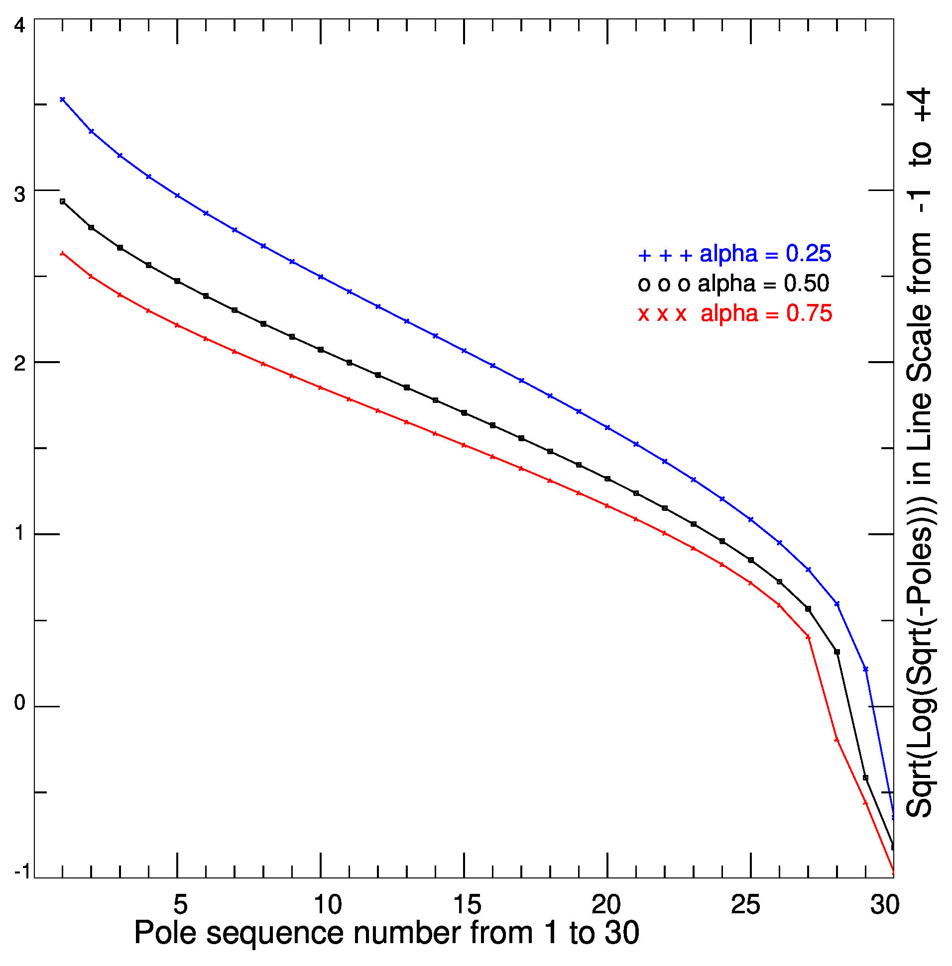
An inherent property of the BURA methods is the exponential clustering of the poles and roots of the corresponding best uniform rational approximation [36], see also [13,37]. Here, we will use the inequality

$${\displaystyle \sqrt{-\frac{1}{{\tilde{d}}_1}}\ge c_d{e}^{-c_{de}k}}$$

(39)

with positive constants $c_d$ and $c_{de}$ that can only depend on the fractional power $\alpha$.

The exponential decrease of $-1/{\tilde{d}}_i$ with increasing i for $k=30$ is shown in Figure 2, where the influence of $\alpha$ is also illustrated. In a local neighborhood of k, we note a zone of faster decrease. However, this feature is not essential for the estimation of $-1/{\tilde{d}}_1$, taking into account the global monotonicity of ${\tilde{d}}_i$. The BRASIL software [33] is used to calculate ${\tilde{d}}_i$, see also [38].

Figure 2. Behavior of $ln\sqrt{-{\displaystyle \frac{1}{{\tilde{d}}_i}}}$ for $1i\in \{1,2,\dots ,30\}$ and $\alpha \in \{0.25,0.50,0.75\}$.

Lemma 4.

Let

$${\displaystyle L\ge \frac{1}{ln(1/\sigma )}\left[ln\frac{1}{{\lambda }_1{c}_d}+c_{de}k\right].}$$

(40)

Then, the scale resolution condition (37) is satisfied.

Proof. 

We write (40) in the form

$$ln{\displaystyle \frac{1}{{\lambda }_1{c}_d}}+c_{de}k\le Lln(1/\sigma ).$$

Then

$${\displaystyle \frac{1}{{\lambda }_1{c}_d}{e}^{c_{de}k}\le {(1/\sigma )}^L}$$

and therefore

$${\sigma }^L\le {\lambda }_1{c}_d{e}^{-c_{de}k}.$$

(41)

Thus, from (41) and (39) we obtain that (37) is satisfied. □

Corollary 1.

The scale resolution condition requires that the number of levels L in the geometrically refined mesh ${\mathcal{T}}_{geo,\sigma }^{L,n}$ be large enough to provide the necessary $hp$ FEM accuracy to the ${\epsilon }_i^2$-perturbed reaction-diffusion problems that arise in the BURA-SD method. It follows from Lemma 4 that there exists a constant $c_k>$ that can only depend on α, so the scale resolution condition is satisfied if

$$L=\lceil c_k\rceil k.$$

(42)

We will now derive a sufficient condition for the degree k of BURA-SD to guarantee balancing of the terms on the right-hand side of the error estimate (38). First, the BURA-SD and h FEM errors are balanced if

$$e^{-2\pi \sqrt{\alpha k}}\sim k{p}^9{\sigma }^{(1+\beta )n}.$$

Therefore,

$$\sqrt{k}\sim lnkp+n,$$

and consequently

$$k\sim {(lnkp+n)}^2.$$

(43)

Analogously, the sufficient condition for balancing the BURA-SD and p FEM errors has the form

$$e^{-2\pi \sqrt{\alpha k}}\sim k{p}^9{e}^{-\gamma p}.$$

Then,

$$\sqrt{k}\sim lnkp+p,$$

and consequently

$$k\sim {(lnkp+p)}^2.$$

(44)

Using (43) and (44) we obtain the following lemma.

Lemma 5.

Let the scale resolution condition (37) be satisfied and let

$$k=n^2+p^2.$$

Then,

$$\left|\right|u-{\widehat{u}}_h{\left|\right|}_{H_1}\le C_e(n^2+p^2)p^9\left({\sigma }^{(1-\beta )n}+e^{-\gamma p}\right).$$

Similar to Lemma 3, the constants $C_e,\gamma >0,\beta \in [0,1)$ depend only on the data $a\left(x\right), f\left(x\right)$ and on the macrotriangulation ${\mathcal{T}}_H$.

We conclude our analysis with the following theorem.

Theorem 2.

Let $\Omega \subset {\mathbb{R}}^2$ be a curvilinear polygon with mesh ${\mathcal{T}}_{geo,\sigma }^{L,n}$ constructed according to assumptions (A1–A5). Then, there exist a mesh refinement parameter $\sigma \in (0,1)$, BURA-SD degree k, and constants $C_e$, $C_c$, $\gamma >0$, $\beta \in [0,1)$ (depending only on the data $a\left(x\right)$, $f\left(x\right)$, and on the macro-triangulation ${\mathcal{T}}_H$), such that the following error estimate holds

$$\left|\right|u-{\widehat{u}}_h{\left|\right|}_{H_1}\le C_e(n^2+p^2)p^9\left({\sigma }^{(1-\beta )n}+e^{-\gamma p}\right)$$

(45)

and the computational complexity is bounded by

$${\mathcal{N}}_{\mathit{BURA}}\le C_c{p}^{4}L(L^2+n).$$

(46)

Proof. 

The error estimate (45) follows directly from Lemma 5. Now, to prove the computational complexity estimate (46) we analyze the implementation of the BURA-SD method. It involves solving k linear systems with the sparse SPD matrices $\mathbb{S}-{\lambda }_{1,h}{\tilde{d}}_i\mathbb{M}\in {\mathbb{R}}^{N\times N}$, $i=1,2,\cdots ,k$. We will assume that a suitable fast preconditioned iterative solver is used for this purpose. For example, such a multigrid preconditioner for the p-hierarchical basis finite element method is proposed in [30]. The number of multigrid iterations $n_{it}^{\mathit{MG}}=O\left(1\right)$ is uniformly bounded regardless of p. Then, the following estimate of the computational complexity ${\mathcal{N}}_{\mathit{BURA}}$ of the BURA-SD method holds

$${\mathcal{N}}_{\mathit{BURA}}=O\left(k{p}^{2}N\right),$$

where $p^2$ represents the number of nonzero off-diagonal elements of the matrices. Thus, from (32) we obtain

$${\mathcal{N}}_{\mathit{BURA}}=O\left(k{p}^4(L^2+n)\right),$$

and finally applying (42) we obtain

$${\mathcal{N}}_{\mathit{BURA}}=O\left(p^{4}L(L^2+n)\right).$$

□

6. Concluding Remarks

In this paper, we have developed a new method for the numerical solution of sub-diffusion problems in curvilinear polygons $\Omega \subset {\mathbb{R}}^2$. This means that there are practically no restrictions on the geometry of the bounded computational domain. The spectral definition of the elliptic operator ${\mathcal{A}}^{\alpha }$, $\alpha \in (0,1]$, is used. The proposed methodology allows the construction of a method that fully utilizes the strengths of the $hp$ FEM and new BURA-SD methods. Only less than ten years ago, we did not have the theoretical basis for creating computationally efficient methods and algorithms for large-scale problems of this type.

The error estimate (45) fully reproduces the exponential convergence rate $O({\sigma }^{(1-\beta )n}+e^{-\gamma p})$ of the $hp$ FEM, see (31), which characterizes the case of a standard (local) elliptic boundary value problem. In addition, the developed algorithm providing this accuracy is computationally highly efficient. In this context, we note that taking into account (32), we can write (46) in the compact form ${\mathcal{N}}_{\mathit{BURA}}=O\left(p^{2}LN\right)$. We recall that in constructing the $hp$ FEM patches, we denote by L the number of geometric refinement layers to an edge where n is the number of geometric refinement layers to a corner that is a vertex of the same edge.

Our research is influenced and motivated by the recently published results in [20]. In short, the following steps apply there. The auxiliary elliptic extension equation in $\Omega \times (0,\infty )$ that was originally proposed in [1] is considered. It is first truncated and diagonalized in the expanded variable. The fractional diffusion problem thus reduces to $\mathcal{M}$ decoupled singularly perturbed diffusion-reaction equations in $\Omega$. The $hp$ FEM discretization and error analysis from [35] are then utilized. By the arguments of [14], we can interpret the method of [20] as a rational approximation of ${\mathcal{A}}^{-\alpha }$. In the context of the present paper, the integer $\mathcal{M}$ corresponds to the BURA-SD degree k.

In this work, we elaborated a novel approach to the BURA (here called BURA-SD) approximation of ${\mathcal{A}}^{-\alpha }$ that is adapted to the specifics in the analysis of the $hp$ FEM used. One may wonder whether some other rational approximation can be integrated into this framework instead of BURA-SD. The answer is yes. Alternatively, both pseudo-parabolic extension (AP2 approach) and quadrature integral representation formulas (AP3 approach) can be applied. It is also worth noting that in each of the AP2-AP3 cases, the problem of computational instability that appears at the disorganization step of A1 approach for larger $\mathcal{M}$ is overcome. Compared to all others, the essential advantage of the BURA-based method is that it provides, by definition, the best uniform rational approximation. When applicable, this leads directly to a better computational complexity as well.

The application of a newly developed numerical method for a class of elliptic problems to the corresponding parabolic equations is usually expected to be a direct consequence. Although this is true for standard (local) partial differential equations, this does not hold in the case of space fractional diffusion problems. The reason for this is that multiplying a vector by the matrix ${\mathbb{A}}^{\alpha }$ turns out to be more complicated than solving a system with the same matrix. A systematic analysis of BURA and BURA-based approximations of the fractional powers of sparse SPD matrices was recently presented in [4]. It follows from the results in [4] that the application of the BURA-SD method proposed here for the case of the $hp$ FEM space discretization to parabolic equations will require a thorough analysis of the computational complexity, which will also include the influence of the condition number $\kappa \left(\mathbb{A}\right)$.

The degree of rational approximation k determines the number of auxiliary sparse linear systems to solve in the implementation of the numerical methods for fractional diffusion equations, which we classified here into four groups according to approaches AP1–AP4. This is the argument for using k as a universal measure when estimating computational complexity via $O\left(k\right)$. More recently, a reduced conjugate gradient basis method for fractional diffusion was proposed in [34]. It is shown there that a smaller number of linear systems can be used without the loss of accuracy of the rational approximation. This is also the aim of the earlier work [26], where the so-called reduced multiplicative (BURA-MR) and additive (BURA-AR) methods were presented. Further theoretical analysis is needed to better understand the possible similarities of the apparently quite different approaches explored in [26,34]. In any case, such kinds of results can be used to improve the algorithm and thus to refine the estimate of the computational complexity (46).

The results in [20], and now in the present paper, raise a wide range of questions for future research. Here, we also note the recent work [39], where an a posteriori error estimator for the spectral fractional power of the Laplacian is developed. In this context, we will note such challenging examples as the generalization of currently available results to fractional diffusion problems in three-dimensional polygons, as well as to equations with heterogeneous and anisotropic coefficients. The development of a BURA-based multilevel adaptive scheme is another attractive topic for future research.

In conclusion, the discussions in this paper have been focused on mesh methods and in particular on the $hp$ FEM discretization case. In perspective, however, we are analyzing alternative possibilities to further develop our research in the spirit of meshless methods.