A New Algorithm for Variational Inequality Problems in CAT(0) Spaces

Abstract

Numerous strong and weak convergence results on variational inequality problems are known in the literature. We here study a variational inequality problem by using the viscosity approximation method in the nonlinear CAT(0) space, where some novel theorems are established for strong and $\Delta$-convergent sequences.

1. Introduction

Variational inequalities originate in the pioneering work of the Italian mathematicians Kinderlehrer and Stampacchia [1], who in their early-1960s pioneering work studied free boundary problems arising in elasticity theory and mechanics by using the variational inequality as an analytic tool. Between 1960 and 1975, many foundational articles appeared in the literature, highlighting the connection between complementarity problems and variational inequalities. For a history of the earliest developments on variational inequalities, readers are referred to [2,3,4,5,6].

Since 1995, numerous publications were devoted to the reformulation of the nonlinear complementarity problem in terms of the algorithms generated through a globally convergent Newton method. Afterwards, many approximation methods and iterative schemes were established for finding the solutions of variational inequalities and related optimization problems (see [7,8,9] and references therein).

One of the numerical methods for solving variational inequality problems (VIPs) is known as the viscosity approximation method (which generates sequences that strongly converge to particular fixed points [10]), which is further expanded in other areas (see, e.g., [11,12] and the references therein).

In [13,14], the authors presented the strong convergence theorems of the Moudafi’s viscosity approximation methods for an asymptotically nonexpansive nonself mapping in CAT(0) spaces. In [15], the authors performed a convergence analysis of a new type of variational inequality problem (VIP) involving nonself multivalued mappings in CAT(0) spaces via a proximal multivalued Picard-S iteration.

Recent advancements in the field have catalyzed new perspectives, exemplified by pseudomonotone mapping in variational inequality problems [16]. These findings underscore the evolving landscape of variational inequality research.

A metric space $(\Omega ,\delta )$ is called a CAT(0) space (the notion rose to prominence through Gromov; see, e.g., [17], p. 159) if it is geodesically connected. For a systematic study regarding these spaces and their essential role in numerous branches of mathematics, readers are referred to Bridson and Haefliger [18]. Given a metric space $(\Omega ,\delta )$, a mapping $\aleph :[0,\delta (u,v\left)\right]\to \Omega$ is called geodesic if it connects $u\in \Omega$ to $v\in \Omega$ in a way such that $\aleph \left(0\right)=u,$$\aleph \left(\delta \right(u,v\left)\right)=v,$ and $\delta (\aleph \left({ı}_1\right),\aleph \left({ı}_2\right))=|{ı}_1-{ı}_2|$ for any ${ı}_1,{ı}_2\in [0,\delta (u,v)].$

Taking any two distinct points $u,v\in (\Omega ,\delta )$, a geodesic segment from u to v is an isometry $\aleph :[0,\delta (u,v\left)\right]\to \Omega$ with $\aleph \left(0\right)=u$ and $\aleph \left(\delta \right(u,v\left)\right)=v$.

A metric space $(\Omega ,\delta )$ is called a geodesic metric space if any two points in $\Omega$ are connected by a geodesic segment. If there is only one geodesic segment from u to v for all $u,v\in \Omega$, then the metric space $(\Omega ,\delta )$ is uniquely geodesic, and this geodesic segment is indicated by $[u,v]$.

Consider the geodesic metric space $(\Omega ,\delta )$. A geodesic triangle has three points $p_1,p_2,p_3\in \Omega$ and three geodesics $[p_1,p_2],[p_2,p_3],[p_3,p_1]$ denoted by

$▵([p_1,p_2],[p_2,p_3],[p_3,p_1])$. For such a triangle, there is a comparison triangle

 

$\overline{▵}(\overline{p_1},\overline{p_2},\overline{p_3})\subset {\mathbb{R}}^2$ such that:

 

• $\delta (p_1,p_2)=\delta (\overline{p_1},\overline{p_2})$
• $\delta (p_2,p_3)=\delta (\overline{p_2},\overline{p_3})$
• $\delta (p_3,p_1)=\delta (\overline{p_3},\overline{p_1})$.

A CAT($\kappa$) space is a metric space $\Omega$ that is geodesically connected and has every geodesic triangle that is at least as ‘thin’ as its comparison triangle in ${\mathbb{R}}^2$. Consider that $(\Omega ,\delta )$ is a geodesic space. It is a CAT(0) space if for any geodesic triangle $▵\subset \Omega$ and $o_1,o_2\in ▵$ we have $\delta (o_1,o_2)\le \delta (\overline{o_1},\overline{o_2})$, where $\overline{o_1},\overline{o_2}\in \overline{▵}$.

Consider a CAT(0) space. Take three points $l,l_1$, and $l_2$ enclosed by it. If $l_0$ is the center of the segment $[l_1,l_2]$, which is indicated as $\frac{l_1\oplus l_2}{2}$, then the CAT(0) inequality implies

$${\delta }^2\left(l,\frac{l_1\oplus l_2}{2}\right)={\delta }^2(l,l_o)\le \frac{1}{2}{\delta }^2(l,l_1)+\frac{1}{2}{\delta }^2(l,l_2)-\frac{1}{4}{\delta }^2(l_1,l_2).$$

This is referred to as the (CN) inequality of Bruhat and Tits [19].

The idea of quasilinearization for a CAT(0) space $\Omega$ was introduced by Berg and Nikolaev [20]. They called it a vector after denoting a pair $(l,m)\in \Omega \times \Omega$ by $\overrightarrow{lm}$. The quasilinearization map $\langle .,.\rangle :(\Omega \times \Omega )\times (\Omega \times \Omega )\to \mathbb{R}$ is defined by

$$\langle \overrightarrow{cd},\overrightarrow{ef}\rangle =\frac{1}{2}({\delta }^2(c,f)+{\delta }^2(d,e)-{\delta }^2(c,e)-{\delta }^2(d,f)),\mathrm{for}\mathrm{all}c,d,e,f\in \Omega .$$

It can be easily verified that

$$\begin{array}{c}\hfill \langle \overrightarrow{cd},\overrightarrow{ef}\rangle =\langle \overrightarrow{ef},\overrightarrow{cd}\rangle ,\langle \overrightarrow{cd},\overrightarrow{ef}\rangle =-\langle \overrightarrow{dc},\overrightarrow{ef}\rangle ;\end{array}$$

and

$$\begin{array}{ccc}\hfill \langle \overrightarrow{cd},\overrightarrow{cd}\rangle & =& {\delta }^2(c,d),\hfill \end{array}$$

(1)

$$\begin{array}{ccc}\hfill \langle \overrightarrow{cd},\overrightarrow{ef}\rangle & =& \langle \overrightarrow{cw},\overrightarrow{ef}\rangle +\langle \overrightarrow{wd},\overrightarrow{ef}\rangle ,\hfill \end{array}$$

(2)

for all $c,d,e,f,w\in \Omega$.

Complete CAT(0) spaces are often called Hadamard spaces (see [21]). It is well-known that a normed linear space satisfies the (CN) inequality if and only if it satisfies the parallelogram identity, i.e., it is a pre-Hilbert space. Hence, it is not so unusual to have an inner product-like notion in Hadamard spaces.

Remark 1. 

A geodesically connected metric space is a CAT(0) space if and only if it satisfies the Cauchy–Schwarz inequality.

In 2010, by using the concept of quasilinearization and by initiating the concept of pseudometric space, Kakavandi and Amini [22] developed dual space for CAT(0) spaces and studied its relation with the subdifferential.

2. Materials and Methods

We now present some key facts about CAT(0) spaces. Throughout this paper, $\mathcal{H}$ denotes a subset of a CAT(0) space $\Omega$, while $\mathcal{A}$ and $\mathcal{B}$ are operators.

To prove the main results, we first need the following useful lemmas.

Lemma 1 

([21]). Consider a CAT(0) space Ω, $p_1,p_2,z\in \Omega$ and $s\in [0,1]$. Then

(i) 

$\delta (s{p}_1\oplus (1-s)p_2,z)\le s\delta (p_1,z)+(1-s)\delta (p_2,z);$

(ii) 

${\delta }^2(s{p}_1\oplus (1-s)p_2,z)\le s{\delta }^2(p_1,z)+(1-s){\delta }^2(p_2,z)-s(1-s){\delta }^2(p_1,p_2)$.

Lemma 2 

([23]). Consider a CAT(0) space Ω, $p_1,p_2,z\in \Omega$ and $s\in [0,1]$. Then

(i) 

$\delta (s{p}_1\oplus (1-s)p_2,\gamma p_1\oplus (1-\gamma )p_2)=|s-\gamma |\delta (p_1,p_2);$

(ii) 

$\delta (s{p}_1\oplus (1-s)p_2,s{p}_1\oplus (1-s)z)\le (1-s)\delta (p_2,z)$.

Lemma 3 

([24]). Every bounded sequence in a complete CAT(0) space Ω always has a Δ-convergent subsequence.

Lemma 4 

([11]). Assume a CAT(0) space Ω. For any $l\in (0,1)$ and $\varsigma ,\zeta \in \Omega$, let

$${\varsigma }_l=l\varsigma \oplus (1-l)\zeta .$$

Then for all $u,v\in X$,

(i) 

$\langle \overrightarrow{{\varsigma }_{l}u},\overrightarrow{{\varsigma }_{l}v}\rangle \le l\langle \overrightarrow{\varsigma u},\overrightarrow{{\varsigma }_{l}v}\rangle +(1-l)\langle \overrightarrow{\zeta u},\overrightarrow{{\varsigma }_{l}v}\rangle$;

(ii) 

$\langle \overrightarrow{{\varsigma }_{l}u},\overrightarrow{\varsigma v}\rangle \le l\langle \overrightarrow{\varsigma u},\overrightarrow{\varsigma v}\rangle +(1-l)\langle \overrightarrow{\zeta u},\overrightarrow{\varsigma v}\rangle \mathit{and}$

$\langle \overrightarrow{{\varsigma }_{l}u},\overrightarrow{\zeta v}\rangle \le l\langle \overrightarrow{\varsigma u},\overrightarrow{\zeta v}\rangle +(1-l)\langle \overrightarrow{\zeta u},\overrightarrow{\zeta v}\rangle .$

Lemma 5 

([11]). Assume that Ω is a CAT(0) space. Consider a closed convex subset $\varnothing \ne \mathcal{H}\subset \Omega .$ Let $\mathcal{T}:\mathcal{H}\to \Omega$ be an asymptotically nonexpansive mapping. If ${\xi }_{\wp }\rightharpoonup \xi$ and $\delta ({\xi }_{\wp },\mathcal{T}{\xi }_{\wp })\to 0$, then $\xi =\mathcal{T}\xi$.

3. $\mathbf{\Pi }$-Duality Mapping and Some Crucial Lemmas

In this section, we define $\Pi$-duality mapping and present some lemmas used for proving our main results. According to [12], we define the following concepts in the setting of CAT(0) space.

Assume a CAT(0) space $\Omega$ and $\Pi :{\Omega }^{*}\to \mathcal{H}$.

• A mapping $\mathcal{P}:\Omega \to \mathcal{H}$ having the following property is known as sunny if

  $$\mathcal{P}(s\varsigma \oplus (1-s\left)\mathcal{P}\varsigma \right)=\mathcal{P}\varsigma ,\varsigma \in \Omega ,s\ge 0,$$

  whenever $s\varsigma \oplus (1-s)\mathcal{P}\varsigma \in \Omega$.

Example 1. 

Consider the mapping $\mathcal{P}:R\to R$ defined by $\mathcal{P}\left(\xi \right)=\xi$ where $\xi \in R$. For any $\xi \in R$ and $s\ge 0$

$$\mathcal{P}[s\xi +(1-s\left)\right(\xi \left)\right]=s\xi +(1-s)\xi =\xi =\mathcal{P}\left(\xi \right)$$

• A mapping $j:\Omega \to {\Omega }^{*}$ is called the duality mapping with regard to $\Pi$ if for any $s,v\in \Omega$

  $$\langle \overrightarrow{sv},\overrightarrow{\Pi j\left(t\right)\Pi j\left(z\right)}\rangle =\delta (s,v)\delta (\Pi j\left(t\right),\Pi j\left(z\right)).$$

Example 2. 

Consider $\Omega =R$ with the usual Euclidean distance $\delta (\xi ,\eta )=|\xi -\eta |$. We need to find a mapping $j:R\to R$ such that $\langle \overrightarrow{sv},\overrightarrow{\Pi j\left(t\right)\Pi j\left(z\right)}\rangle =\delta (s,v)\delta (\Pi j\left(t\right),\Pi j\left(z\right))$. First, let us consider the mapping $j\left(\xi \right)=-\xi$ with $\Pi j\left(\xi \right)=-\xi$. By quasilinearization, one obtains

$$\begin{array}{ccc}\hfill \langle \overrightarrow{sv},\overrightarrow{(-t)(-z)}\rangle & =& \frac{1}{2}[{\delta }^2(s,-z)+{\delta }^2(v,-t)-{\delta }^2(s,-t)-{\delta }^2(v,-z)]\hfill \\ & =& \frac{1}{2}[{(s+z)}^2+{(v+t)}^2-{(s+t)}^2-{(v+z)}^2]\hfill \\ & =& \frac{1}{2}[2sz+2vt-2st-2vz]\hfill \\ & =& sz+vt-st-vz\hfill \\ & =& |s-v|.|t-z|\hfill \\ & =& \delta (s,v)\delta (t,z)\hfill \\ & =& \delta (s,v)\delta (\Pi j(t),\Pi j(z\left)\right)\hfill \end{array}$$

• A mapping $j:\Omega \to {\Omega }^{*}$ is called the normalized duality mapping (abbreviated as ND-map) with respect to $\Pi$ if

  $$\langle \overrightarrow{sv},\overrightarrow{\Pi j\left(s\right)\Pi j\left(v\right)}\rangle ={\delta }^2(s,v)={\delta }^2(\Pi j\left(s\right),\Pi j\left(v\right)).$$

• An operator $\mathcal{A}:\mathcal{H}\to \Omega$ is called accretive if

  $$\langle \overrightarrow{\mathcal{A}\varsigma \mathcal{A}\zeta },\overrightarrow{\Pi j\left(\varsigma \right)\Pi j\left(\zeta \right)}\rangle \ge 0\mathrm{for}\mathrm{all}\varsigma ,\zeta \in \mathcal{H}.$$

  where $\Pi j$ is the ND-map on $\Omega$.

• For $\alpha >0$, an operator $\mathcal{A}:\mathcal{H}\to \Omega$ is called $\alpha$-inverse strongly accretive (abbreviated as $\alpha$-ISA) if

  $$\langle \overrightarrow{\mathcal{A}\varsigma \mathcal{A}\zeta },\overrightarrow{\Pi j\left(\varsigma \right)\Pi j\left(\zeta \right)}\rangle \ge \alpha {\delta }^2\left(\mathcal{A}\varsigma ,\mathcal{A}\zeta \right)\mathrm{for}\mathrm{all}\varsigma ,\zeta \in \mathcal{H}.$$

Example 3. 

Let $\Omega =R$ and $\mathcal{H}=\{\xi \in R:0<\xi <1\}$. Define the functions $\Pi j\left(\xi \right)=\frac{cos\left(\xi \right)}{2}$ and $\mathcal{A}\left(\xi \right)=\frac{1}{2}log(1+{\xi }^2)$. Let $\varsigma =0.1$ and $\zeta =0.3$. Then $\Pi j\left(0.1\right)=0.49999923845$ and $\Pi j\left(0.3\right)=0.499993146$. Furthermore, $\mathcal{A}\left(0.1\right)=0.0021606$ and $\mathcal{A}\left(0.3\right)=0.01871324$. This implies

$$\begin{array}{ccc}& & \langle \overrightarrow{\mathcal{A}\varsigma \mathcal{A}\zeta },\overrightarrow{\Pi j\left(\varsigma \right)\Pi j\left(\zeta \right)}\rangle \hfill \\ & & =\frac{1}{2}({\delta }^2(\mathcal{A}\varsigma ,\Pi j\left(\zeta \right))+{\delta }^2(\mathcal{A}\zeta ,\Pi j\left(\varsigma \right))-{\delta }^2(\mathcal{A}\varsigma ,\Pi j\left(\varsigma \right))-{\delta }^2(\mathcal{A}\zeta ,\Pi j\left(\zeta \right)))\hfill \\ & & =0.0026\ge 0.\hfill \end{array}$$

That implies that $\mathcal{A}$ is accretive. By taking $\alpha =0.1$, we obtain that $\mathcal{A}$ is an α-ISA operator.

Let $\mathcal{C}$ be a subset of a Banach space $\mathcal{S}$. The usual VIP in a Banach space $\mathcal{S}$ is to find $i\in \mathcal{C}\subset \mathcal{S}$ if there exists $J:\mathcal{S}\to 2^{{\mathcal{S}}^{*}}$ an ND-map on $\mathcal{S}$ and $j(\xi -i)\in J(\xi -i)$ such that

$$\langle \mathcal{A}i,j(\xi -i)\rangle \ge 0,\forall \xi \in \mathcal{C}.$$

In 2010, a structure was proposed by Yao et al. [25] to find $(\varsigma ,\zeta )\in \mathcal{C}\times \mathcal{C}$ such that

$$\begin{array}{c}\hfill \left\{\begin{array}{c}\langle \mathcal{A}\zeta +\varsigma -\zeta ,j(\xi -\varsigma )\rangle \ge 0,\forall \xi \in \mathcal{C},\hfill \\ \langle \mathcal{B}\varsigma +\zeta -\varsigma ,j(\xi -\zeta )\rangle \ge 0,\forall \xi \in \mathcal{C},\hfill \end{array}\right.\end{array}$$

which is known as the generalized variational inequality system (abbreviated as GVIS) in Banach spaces. Wang and Pan et al. [12] formulated the theorem regarding the strong convergence of the subsequent iterative scheme:

$$\begin{array}{c}\hfill \left\{\begin{array}{c}{w}_n={\mathcal{P}}_{\mathcal{H}}(I-\mu \mathcal{B}){\xi }_n,\hfill \\ z_n={\mathcal{P}}_{\mathcal{H}}(I-\lambda \mathcal{A})(t{\xi }_n+(1-t)w_n),\hfill \\ u_n={\varpi }_n{\xi }_n+(1-{\varpi }_n)z_n,\hfill \\ {\xi }_{n+1}={\aleph }_{n}f\left({\xi }_n\right)+{\Re }_n{\xi }_n+{\gamma }_n{\mathcal{T}}^n{u}_n,\hfill \end{array}\right.\end{array}$$

for the following problem about the GVIS:

$$\begin{array}{c}\hfill \left\{\begin{array}{c}\langle (I-\lambda \mathcal{A})(t{\xi }^{†}+(1-t){\iota }^{†})-{\xi }^{†},j(\xi -{\xi }^{†})\rangle \le 0,\forall \xi \in \mathcal{C},\hfill \\ \langle (I-\mu \mathcal{B}){\xi }^{†}-{\iota }^{†},j(\xi -{\iota }^{†})\rangle \le 0,\forall \xi \in \mathcal{C}.\hfill \end{array}\right.\end{array}$$

The motivation for this work is driven by the natural progression from linear to nonlinear settings, the broad applicability and theoretical richness of CAT(0) spaces, and the practical need for efficient algorithms in complex, real-world scenarios. This research aims to fill the gap by providing a robust algorithm that can tackle variational inequality problems within the flexible and encompassing framework of CAT(0) spaces. While significant progress has been made in solving variational inequality problems in linear and Euclidean spaces, many real-world problems inherently exhibit nonlinear characteristics. CAT(0) spaces, which generalize Euclidean spaces to a broader class of geodesic metric spaces, provide a rich and flexible framework for addressing such nonlinear problems. Extending the theory of VIPs to CAT(0) spaces can lead to new insights and theoretical advancements in the study of variational inequalities.

Inspired and convinced by researchers’ findings, we implemented the subsequent iterative approach within a CAT(0) space to demonstrate strong convergence:

$$\left\{\begin{array}{c}{w}_n={\mathcal{P}}_{\mathcal{H}}[(1-\mu )I\oplus \mu \mathcal{B}]{\xi }_n,\hfill \\ z_n={\mathcal{P}}_{\mathcal{H}}[(1-\lambda )I\oplus \lambda \mathcal{A}][t{\xi }_n\oplus (1-t)w_n],\hfill \\ u_n={\varpi }_n{\xi }_n\oplus (1-{\varpi }_n)z_n,\hfill \\ {\xi }_{n+1}={\aleph }_{n}f\left({\xi }_n\right)\oplus (1-{\aleph }_n)[\frac{{\Re }_n}{1-{\aleph }_n}{\xi }_n\oplus (1-\frac{{\Re }_n}{1-{\aleph }_n}){\mathcal{T}}^n{u}_n],\hfill \end{array}\right.$$

(3)

where $\left\{{\aleph }_n\right\},\left\{{\Re }_n\right\},\left\{{\gamma }_n\right\},\left\{{\varpi }_n\right\}\subset (0,1)$. The sequence $\left\{{\xi }_n\right\}$ defined by (3) satisfies the conditions ${\aleph }_n+{\Re }_n+{\gamma }_n=1$, ${lim}_{n\to \infty }{\aleph }_n=0$, $k_n-1=ϵ{\aleph }_n$, and $0<ϵ<1-\rho$. Also, the conditions ${lim}_{n\to \infty }{\Re }_n=0$, ${lim}_{n\to \infty }{\aleph }_{n+1}=0$, ${lim}_{n\to \infty }{\Re }_{n+1}=0$, as well as $0<{lim\; inf}_{n\to \infty }{\Re }_n\le {lim\; sup}_{n\to \infty }{\Re }_n<1$, ${lim}_{n\to \infty }|{\varpi }_{n+1}-2{\varpi }_{n+1}{\varpi }_n+{\varpi }_n|=0$ for the following GVIS in CAT(0) spaces:

$$\begin{array}{c}\hfill \left\{\begin{array}{cc}& \langle (\overrightarrow{[(1-\lambda )I\oplus \lambda \mathcal{A}][\tau {\xi }^{†}\oplus (1-\tau ){\eta }^{†}]){\xi }^{†}},\overrightarrow{\Pi j\left(\xi \right)\Pi j\left({\xi }^{†}\right)}\rangle \le 0,\hfill \\ & \langle \overrightarrow{[(1-\mu )I\oplus \mu \mathcal{B}]{\xi }^{†}},\overrightarrow{\Pi j\left(\xi \right)\Pi j\left({\eta }^{†}\right)}\rangle \le 0.\hfill \end{array}\right.\end{array}$$

The lemmas below also are used for proving our main result.

Lemma 6. 

Assume j is the ND-map on a CAT(0) space Ω. Let $\mathcal{P}:\Omega \to \mathcal{H}$ be a retract and assume a point $z\in \mathcal{H}$ that satisfies $\delta (z,\xi )=inf\left\{\delta \right(\eta ,\xi );\eta \in \mathcal{H}\}$ and $\langle \overrightarrow{\eta z},\overrightarrow{\Pi j\left(z\right)\Pi j\left(\xi \right)}\rangle \ge 0$ for all $\eta \in \mathcal{H}$. Then next declarations are identical:

(a) 

${\delta }^2(\mathcal{P}\xi ,\mathcal{P}\eta )\le \langle \overrightarrow{\xi \eta },\overrightarrow{\Pi j\left(\mathcal{P}\xi \right)\Pi j\left(\mathcal{P}\eta \right)}\rangle$;

(b) 

$\langle \overrightarrow{\xi \mathcal{P}\xi },\overrightarrow{\Pi j\left(\eta \right)\Pi j\left(\mathcal{P}\xi \right)}\rangle \le 0$;

(c) 

$\mathcal{P}$ is sunny and nonexpansive.

Proof. 

$\left(a\right)\Rightarrow \left(b\right)$. Suppose that ${\delta }^2(\mathcal{P}\xi ,\mathcal{P}\eta )\le \langle \overrightarrow{\xi \eta },\overrightarrow{\Pi j\left(\mathcal{P}\xi \right)\Pi j\left(\mathcal{P}\eta \right)}\rangle$ holds. Let $\xi \in \Omega$. Replacing $\eta$ by $\eta =\mathcal{P}\eta$ in (a), we have

$$\begin{array}{ccc}\hfill {\delta }^2(\mathcal{P}\xi ,{\mathcal{P}}^2\eta )& \le & \langle \overrightarrow{\xi \mathcal{P}\eta },\overrightarrow{\Pi j\left(\mathcal{P}\xi \right)\Pi j\left({\mathcal{P}}^2\eta \right)}\rangle \hfill \\ \hfill {\delta }^2(\mathcal{P}\xi ,\eta )& \le & \langle \overrightarrow{\xi \mathcal{P}\eta },\overrightarrow{\Pi j\left(\mathcal{P}\xi \right)\Pi j\left(\eta \right)}\rangle .\hfill \end{array}$$

By Equation (2)

$$\begin{array}{ccc}\hfill \langle \overrightarrow{\xi \mathcal{P}\xi },\overrightarrow{\Pi j\left(\mathcal{P}\xi \right)\Pi j\left(\eta \right)}\rangle & =& \langle \overrightarrow{\xi \mathcal{P}\left(\eta \right)},\overrightarrow{\Pi j\left(\mathcal{P}\xi \right)\Pi j\left(\eta \right)}\rangle -\langle \overrightarrow{\mathcal{P}\left(\xi \right)\eta },\overrightarrow{\Pi j\left(\mathcal{P}\xi \right)\Pi j\left(\eta \right)}\rangle \hfill \\ & \ge & {\delta }^2(\mathcal{P}\left(\xi \right),\eta )-{\delta }^2(\mathcal{P}\left(\xi \right),\eta )\hfill \\ & \ge & 0.\hfill \end{array}$$

By the property of quasilinearization, we obtain

$$\begin{array}{ccc}\hfill \langle \overrightarrow{\xi \mathcal{P}\xi },\overrightarrow{\Pi j\left(\eta \right)\Pi j\left(\mathcal{P}\xi \right)}\rangle & \le & 0.\hfill \end{array}$$

$\left(b\right)\Rightarrow \left(a\right)$. Let $\xi ,\eta \in \Omega$. Then $\mathcal{P}\xi ,\mathcal{P}\eta \in \mathcal{H}$, we have

$$\begin{array}{c}\hfill \langle \overrightarrow{\xi \mathcal{P}\xi },\overrightarrow{\Pi j\left(\mathcal{P}\eta \right)\Pi j\left(\mathcal{P}\xi \right)}\rangle \le 0\mathrm{and}\langle \overrightarrow{\eta \mathcal{P}\eta },\overrightarrow{\Pi j\left(\mathcal{P}\xi \right)\Pi j\left(\mathcal{P}\eta \right)}\rangle \le 0.\end{array}$$

$$\begin{array}{ccc}\hfill {\delta }^2(\mathcal{P}\xi ,\mathcal{P}\eta )& =& \langle \overrightarrow{\mathcal{P}\xi \mathcal{P}\eta },\overrightarrow{\Pi j\left(\mathcal{P}\xi \right)\Pi j\left(\mathcal{P}\eta \right)}\rangle \hfill \\ & =& \langle \overrightarrow{\mathcal{P}\xi \xi },\overrightarrow{\Pi j\left(\mathcal{P}\xi \right)\Pi j\left(\mathcal{P}\eta \right)}\rangle +\langle \overrightarrow{\xi \mathcal{P}\eta },\overrightarrow{\Pi j\left(\mathcal{P}\xi \right)\Pi j\left(\mathcal{P}\eta \right)}\rangle \hfill \\ & \le & \langle \overrightarrow{\xi \mathcal{P}\eta },\overrightarrow{\Pi j\left(\mathcal{P}\xi \right)\Pi j\left(\mathcal{P}\eta \right)}\rangle \hfill \\ & =& \langle \overrightarrow{\xi \eta },\overrightarrow{\Pi j\left(\mathcal{P}\xi \right)\Pi j\left(\mathcal{P}\eta \right)}\rangle +\langle \overrightarrow{\eta \mathcal{P}\eta },\overrightarrow{\Pi j\left(\mathcal{P}\xi \right)\Pi j\left(\mathcal{P}\eta \right)}\rangle \hfill \\ & \le & \langle \overrightarrow{\xi \eta },\overrightarrow{\Pi j\left(\mathcal{P}\xi \right)\Pi j\left(\mathcal{P}\eta \right)}\rangle .\hfill \end{array}$$

$\left(b\right)\Rightarrow \left(c\right)$. Suppose $\mathcal{P}$ is a retraction such that $\langle \overrightarrow{\xi \mathcal{P}\xi },\overrightarrow{\Pi j\left(\eta \right)\Pi j\left(\mathcal{P}\xi \right)}\rangle \le 0$; we have to show that $\mathcal{P}$ is sunny and nonexpansive.

Claim I. For $\xi ,\gamma \in \Omega$, from $\left(b\right)$, we obtain

$$\begin{array}{c}\hfill \langle \overrightarrow{\xi \mathcal{P}\xi },\overrightarrow{\Pi j\left(\mathcal{P}\xi \right)\Pi j\left(\mathcal{P}\gamma \right)}\rangle \ge 0\mathrm{and}\langle \overrightarrow{\gamma \mathcal{P}\gamma },\overrightarrow{\Pi j\left(\mathcal{P}\gamma \right)\Pi j\left(\mathcal{P}\xi \right)}\rangle \ge 0.\end{array}$$

Hence,

$$\begin{array}{ccc}\hfill {\delta }^2(\mathcal{P}\xi ,\mathcal{P}\gamma )& =& \langle \overrightarrow{\mathcal{P}\xi \mathcal{P}\gamma },\overrightarrow{\Pi j\left(\mathcal{P}\xi \right)\Pi j\left(\mathcal{P}\gamma \right)}\rangle \hfill \\ & =& \langle \overrightarrow{\mathcal{P}\xi \xi },\overrightarrow{\Pi j\left(\mathcal{P}\xi \right)\Pi j\left(\mathcal{P}\gamma \right)}\rangle +\langle \overrightarrow{\xi \gamma },\overrightarrow{\Pi j\left(\mathcal{P}\xi \right)\Pi j\left(\mathcal{P}\gamma \right)}\rangle \hfill \\ & & +\langle \overrightarrow{\gamma \mathcal{P}\gamma },\overrightarrow{\Pi j\left(\mathcal{P}\xi \right)\Pi j\left(\mathcal{P}\gamma \right)}\rangle \hfill \\ & \le & \langle \overrightarrow{\xi \gamma },\overrightarrow{\Pi j\left(\mathcal{P}\xi \right)\Pi j\left(\mathcal{P}\gamma \right)}\rangle .\hfill \end{array}$$

So, $\mathcal{P}$ is nonexpansive.

Claim II. For $\xi \in \Omega$, set ${\xi }_t=t\xi \oplus (1-t)\mathcal{P}\xi$ for all $t>0$. Because $\Omega$ is convex, it follows that ${\xi }_t\in \Omega$ for all $t\in [0,1]$. Hence

$$\begin{array}{c}\hfill \langle \overrightarrow{\xi \mathcal{P}\xi },\overrightarrow{\Pi j\left(\mathcal{P}\xi \right)\Pi j\left(\mathcal{P}{\xi }_t\right)}\rangle \ge 0\mathrm{and}\langle \overrightarrow{{\xi }_t\mathcal{P}{\xi }_t},\overrightarrow{\Pi j\left(\mathcal{P}{\xi }_t\right)\Pi j\left(\mathcal{P}\xi \right)}\rangle \ge 0.\end{array}$$

Because

$$\begin{array}{ccc}\hfill \langle \overrightarrow{{\xi }_t\mathcal{P}\xi },\overrightarrow{\Pi j\left(\mathcal{P}\xi \right)\Pi j\left(\mathcal{P}{\xi }_t\right)}\rangle & =& \delta ({\xi }_t,\mathcal{P}\xi )\delta (\Pi j\left(\mathcal{P}\xi \right),\Pi j\left(\mathcal{P}{\xi }_t\right))\hfill \\ & =& \delta (t\xi \oplus (1-t)\mathcal{P}\xi ,\mathcal{P}\xi )\delta (\Pi j\left(\mathcal{P}\xi \right),\Pi j\left(\mathcal{P}{\xi }_t\right))\hfill \\ & \le & [t\delta (\xi ,\mathcal{P}\xi )+(1-t)\delta (\mathcal{P}\xi ,\mathcal{P}\xi )]\delta (\Pi j\left(\mathcal{P}\xi \right),\Pi j\left(\mathcal{P}{\xi }_t\right))\hfill \\ & =& t\delta (\xi ,\mathcal{P}\xi )\delta (\Pi j\left(\mathcal{P}\xi \right),\Pi j\left(\mathcal{P}{\xi }_t\right))\hfill \\ & =& t\langle \overrightarrow{\xi \mathcal{P}\xi },\overrightarrow{\Pi j\left(\mathcal{P}\xi \right)\Pi j\left(\mathcal{P}{\xi }_t\right)}\rangle \ge 0,\hfill \end{array}$$

so we have

$$\langle \overrightarrow{{\xi }_t\mathcal{P}\xi },\overrightarrow{\Pi j\left(\mathcal{P}\xi \right)\Pi j\left(\mathcal{P}{\xi }_t\right)}\rangle \ge 0.$$

Now,

$$\begin{array}{ccc}\hfill {\delta }^2(\mathcal{P}\xi ,\mathcal{P}{\xi }_t)& =& \langle \overrightarrow{\mathcal{P}\xi \mathcal{P}{\xi }_t},\overrightarrow{\Pi j\left(\mathcal{P}\xi \right)\Pi j\left(\mathcal{P}{\xi }_t\right)}\rangle \hfill \\ & =& \langle \overrightarrow{\mathcal{P}\xi {\xi }_t},\overrightarrow{\Pi j\left(\mathcal{P}\xi \right)\Pi j\left(\mathcal{P}{\xi }_t\right)}\rangle +\langle \overrightarrow{{\xi }_t\mathcal{P}{\xi }_t},\overrightarrow{\Pi j\left(\mathcal{P}\xi \right)\Pi j\left(\mathcal{P}{\xi }_t\right)}\rangle \hfill \\ & =& -\langle \overrightarrow{{\xi }_t\mathcal{P}\xi },\overrightarrow{\Pi j\left(\mathcal{P}\xi \right)\Pi j\left(\mathcal{P}{\xi }_t\right)}\rangle +\langle \overrightarrow{{\xi }_t\mathcal{P}{\xi }_t},\overrightarrow{\Pi j\left(\mathcal{P}\xi \right)\Pi j\left(\mathcal{P}{\xi }_t\right)}\rangle \hfill \\ & \le & 0.\hfill \end{array}$$

Thus, $\mathcal{P}\xi =\mathcal{P}{\xi }_t$. Therefore, $\mathcal{P}$ is sunny.

$\left(c\right)\Rightarrow \left(b\right)$. Suppose the retraction $\mathcal{P}$ is both sunny and nonexpansive. Let $\xi \in \Omega$ and $\mathcal{P}\xi \in \mathcal{H}$ and put $\mathcal{P}\xi =z$. $M=\{t\xi \oplus (1-t)z:t\ge 0\}$ is convex. If $v\in M$, then

$$\delta (y,z)=\delta (\mathcal{P}y,\mathcal{P}v)\le \delta (y,v).$$

By our assumption, we obtain

$$\langle \overrightarrow{\xi \mathcal{P}\xi },\overrightarrow{\Pi j\left(\eta \right)\Pi j\left(\mathcal{P}\xi \right)}\rangle \le 0,$$

which ends the proof. □

Lemma 7. 

Assume Ω is a CAT(0) space. Consider any two bounded sequences $\left\{y_{\wp }\right\}$ and $\left\{x_{\wp }\right\}$ in Ω and let $\left\{{\beta }_{\wp }\right\}\in [0,1]$ be a sequence with $0<{lim\; inf}_{\wp \to \infty }{\upsilon }_{\wp }\le {lim\; sup}_{\wp \to \infty }{\beta }_{\wp }<1$. Let

$$\underset{\wp \to \infty }{lim\; inf}|\delta ({\varpi }_{\wp +ȷ},{\varrho }_{\wp })-(1+{\upsilon }_{\wp }+{\upsilon }_{\wp +1}+\dots +{\upsilon }_{\wp +ȷ-1})q|=0,$$

(4)

hold for all $ȷ\in N$. If $x_{\wp +1}=(1-{\beta }_{\wp })x_{\wp }\oplus {\beta }_{\wp }{p}_{\wp }$ for all $\wp \ge 0$ and ${lim\; sup}_{\wp \to \infty }(\delta (p_{\wp +1},p_{\wp })-\delta (x_{\wp +1},x_{\wp }))\le 0$, then ${lim}_{\wp \to \infty }\delta (p_{\wp },x_{\wp })=0.$

Proof. 

We put $g={lim\; inf}_{\wp }{\upsilon }_{\wp }>0$, $M=2sup\{\delta ({\varrho }_{\wp },x_{\wp }),\wp \in N\}<\infty$, and $q={lim\; sup}_{\wp }\delta ({\sigma }_{\wp },{\varrho }_{\wp })<\infty$. We assume $q>0$. Then fix $k\in N$ with $(1+ka)q>M$. By Equation (4), we have

$$\underset{\wp \to \infty }{lim\; inf}|\delta ({\varpi }_{\wp +ȷ},{\varrho }_{\wp })-(1+{\upsilon }_{\wp }+{\upsilon }_{\wp +1}+\dots +{\upsilon }_{\wp +ȷ+1})q|=0.$$

Thus, there exists a subsequence $\left\{{\wp }_{\ell }\right\}$ of a sequence $\{\wp \}$ in N such that

$$\underset{\ell \to \infty }{lim\; inf}|\delta ({\varpi }_{{\wp }_{\ell }+ȷ},{\varrho }_{{\wp }_{\ell }})-(1+{\upsilon }_{{\wp }_{\ell }}+{\upsilon }_{{\wp }_{\ell }+1}+\dots +{\upsilon }_{{\wp }_{\ell }+ȷ+1})q|=0.$$

The limit $\delta ({\varpi }_{{\wp }_{\ell }+ȷ},{\varrho }_{{\wp }_{\ell }})$ exists, and the limits of $\left\{{\upsilon }_{\wp +ı}\right\}$ exist for all $ı\in \{0,1,\dots ,ȷ-1\}$. Put ${\beta }_{ı}={lim}_{\ell }{\upsilon }_{{\wp }_{\ell }+ı}$ for $ı\in \{0,1,\dots ,ȷ-1\}$. It is obvious that ${\beta }_{ı}\ge g$ for all $ı\in \{0,1,\dots ,ȷ-1\}$. We have

$$\begin{array}{ccc}\hfill M& <& (1+kg)q\hfill \\ & =& (1+{\beta }_0+{\beta }_1+\dots +{\beta }_{\wp -1})d\hfill \\ & =& \underset{\ell \to \infty }{lim}(1+{\upsilon }_{{\wp }_{\ell }}+{\upsilon }_{{\wp }_{\ell }+1}+\dots +{\upsilon }_{{\wp }_{\ell }+ȷ-1})q\hfill \\ & =& \underset{\ell \to \infty }{lim}\delta ({\varpi }_{{\wp }_{\ell }+ȷ},{\varrho }_{{\wp }_{\ell }})\hfill \\ & \le & \underset{\wp \to \infty }{lim\; sup}\delta ({\varpi }_{\wp +ȷ},{\varrho }_{\wp })\hfill \\ & \le & M.\hfill \end{array}$$

This is a contradiction. Therefore, $q=0$. □

Lemma 8. 

Assume Ω is a CAT(0) space. Consider a closed convex subset $\varnothing \ne \mathcal{H}\subset \Omega$. If the operator $\mathcal{A}:\mathcal{H}\to \Omega$ is α-ISA, then we have

$$\begin{array}{ccc}\hfill {\delta }^2([(1-\lambda )I\oplus \lambda \mathcal{A}]\xi ,[(1-\lambda )I\oplus \lambda \mathcal{A}]\eta )& \le & {\delta }^2(\xi ,\eta )-2{\lambda }^2\langle \overrightarrow{\mathcal{A}\xi \xi },\overrightarrow{\mathcal{A}\eta \eta }\rangle \hfill \\ & & +{\lambda }^2[{\delta }^2(\mathcal{A}\eta ,\eta )+{\delta }^2(\mathcal{A}\xi ,\xi )],\hfill \end{array}$$

where $\lambda >0$. If $2\langle \overrightarrow{\mathcal{A}\xi \xi },\overrightarrow{\mathcal{A}\eta \eta }\rangle \ge {\delta }^2(\mathcal{A}\eta ,\eta )+{\delta }^2(\mathcal{A}\xi ,\xi )$, then $(1-\lambda )I\oplus \lambda \mathcal{A}$ is nonexpansive.

Proof. 

Let

$$\begin{array}{ccc}\hfill {\delta }^2(u\left(\xi \right),u\left(\eta \right))& =& {\delta }^2([(1-\lambda )I\oplus \lambda \mathcal{A}]\xi ,[(1-\lambda )I\oplus \lambda \mathcal{A}]\eta )\hfill \\ & =& {\delta }^2([(1-\lambda )I\oplus \lambda \mathcal{A}]\xi ,u\left(\eta \right))\hfill \\ & \le & \lambda {\delta }^2(\mathcal{A}\xi ,u\left(\eta \right))+(1-\lambda ){\delta }^2(\xi ,,u\left(\eta \right))-\lambda (1-\lambda ){\delta }^2(\mathcal{A}\xi ,\xi )\hfill \\ & =& \lambda {\delta }^2(u\left(\eta \right),\mathcal{A}\xi )+(1-\lambda ){\delta }^2(u\left(\eta \right),\xi )-\lambda (1-\lambda ){\delta }^2(\mathcal{A}\xi ,\xi ).\hfill \end{array}$$

Now,

$$\begin{array}{ccc}\hfill {\delta }^2(u\left(\eta \right),\mathcal{A}\xi )& =& {\delta }^2([(1-\lambda )I\oplus \lambda \mathcal{A}]\eta ,\mathcal{A}\xi )\hfill \\ & \le & \lambda {\delta }^2(\mathcal{A}\eta ,\mathcal{A}\xi )+(1-\lambda ){\delta }^2(\eta ,\mathcal{A}\xi )-\lambda (1-\lambda ){\delta }^2(\mathcal{A}\eta ,\eta ).\hfill \end{array}$$

Furthermore, we have

$$\begin{array}{ccc}\hfill {\delta }^2(u\left(\eta \right),\xi )& =& {\delta }^2([(1-\lambda )I\oplus \lambda \mathcal{A}]\eta ,\xi )\hfill \\ & \le & \lambda {\delta }^2(\mathcal{A}\eta ,\xi )+(1-\lambda ){\delta }^2(\eta ,\xi )-\lambda (1-\lambda ){\delta }^2(\mathcal{A}\eta ,\eta ),\hfill \end{array}$$

so,

$$\begin{array}{ccc}\hfill {\delta }^2(u\left(\xi \right),u\left(\eta \right))& \le & \lambda [\lambda {\delta }^2(\mathcal{A}\eta ,\mathcal{A}\xi )+(1-\lambda ){\delta }^2(\eta ,\mathcal{A}\xi )-\lambda (1-\lambda ){\delta }^2(\mathcal{A}\eta ,\eta )]\hfill \\ & & +(1-\lambda )[\lambda {\delta }^2(\mathcal{A}\eta ,\xi )+(1-\lambda ){\delta }^2(\eta ,\xi )-\lambda (1-\lambda ){\delta }^2(\mathcal{A}\eta ,\eta )]\hfill \\ & & -\lambda (1-\lambda ){\delta }^2(\mathcal{A}\xi ,\xi )\hfill \\ & \le & {\delta }^2(\eta ,\xi )+{\lambda }^2[{\delta }^2(\mathcal{A}\eta ,\mathcal{A}\xi )-{\delta }^2(\eta ,\mathcal{A}\xi )+{\delta }^2(\mathcal{A}\eta ,\eta )\hfill \\ & & +{\delta }^2(\eta ,\xi )-{\delta }^2(\mathcal{A}\eta ,\xi )+{\delta }^2(\mathcal{A}\xi ,\xi )]+\lambda [{\delta }^2(\eta ,\mathcal{A}\xi )\hfill \\ & & -{\delta }^2(\mathcal{A}\eta ,\eta )-2{\delta }^2(\eta ,\xi )+{\delta }^2(\mathcal{A}\eta ,\xi )-{\delta }^2(\mathcal{A}\xi ,\xi )]\hfill \\ & \le & {\delta }^2(\eta ,\xi )+\lambda [{\delta }^2(\eta ,\xi )+{\delta }^2(\mathcal{A}\xi ,\xi )-{\delta }^2(\mathcal{A}\eta ,\eta )\hfill \\ & & +{\delta }^2(\mathcal{A}\eta ,\xi )-2{\delta }^2(\eta ,\xi )-{\delta }^2(\mathcal{A}\xi ,\xi )]\hfill \\ & & +{\lambda }^2[-2\langle \overrightarrow{\mathcal{A}\xi \xi },\overrightarrow{\mathcal{A}\eta \eta }\rangle +{\delta }^2(\mathcal{A}\eta ,\eta )+{\delta }^2(\mathcal{A}\xi ,\xi )]\hfill \\ & \le & {\delta }^2(\eta ,\xi )-2{\lambda }^2\langle \overrightarrow{\mathcal{A}\xi \xi },\overrightarrow{\mathcal{A}\eta \eta }\rangle +{\lambda }^2[{\delta }^2(\mathcal{A}\eta ,\eta )+{\delta }^2(\mathcal{A}\xi ,\xi )].\hfill \end{array}$$

The proof is complete. □

Lemma 9. 

Assume Ω is a real CAT(0) space. Consider a closed convex subset $\varnothing \ne \mathcal{H}\subset \Omega$. Assume $F\left(\mathcal{T}\right)\ne \varnothing$ with $\mathcal{T}:\mathcal{H}\to \mathcal{H}$ is a nonexpansive mapping. Let $f:\mathcal{H}\to \mathcal{H}$ be a contractive mapping. Define a sequence ${\xi }_s$ as follows: ${\xi }_s=sf\left({\xi }_s\right)\oplus (1-s)\mathcal{T}{\xi }_s,s\in (0,1)$. Then ${\xi }_s$ converges strongly to a point in $F\left(\mathcal{T}\right)$. Assume

$$LIM\delta (f\left(i\right),\xi )\delta (\Pi j\left({\xi }_n\right),\Pi j\left(p\right))\le 0,$$

and

$$\langle ((1-\lambda )I\oplus \lambda f){\xi }_s,\overrightarrow{\Pi j\left(\mathcal{P}\right(f\left)\right)\Pi j\left(p\right)}\rangle \le 0,\forall p\in F\left(\mathcal{T}\right).$$

Suppose $\mathcal{S}:{\prod }_c\to F\left(\mathcal{T}\right)$ is defined as $\mathcal{S}\left(f\right)={lim}_{s\to 0}{\xi }_s,f\in {\prod }_c$, then $\mathcal{P}\left(f\right)$ clarifies the following inequality:

$$\langle ((1-\lambda )I\oplus \lambda f)\mathcal{S}\left(f\right),\overrightarrow{\Pi j\left(\mathcal{P}\right(f)\Pi j(p)}\rangle \le 0,\forall p\in F\left(\mathcal{T}\right).$$

Proof. 

We first show that $\left\{{\xi }_s\right\}$ is bounded.

$$\begin{array}{ccc}\hfill \delta ({\xi }_s,\iota )& =& \delta (sf\left({\xi }_s\right)\oplus (1-s)\mathcal{T}{\xi }_s,\iota )\hfill \\ & \le & s\delta (f\left({\xi }_s\right),\iota )+(1-s)\delta (\mathcal{T}{\xi }_s,\iota )\hfill \\ & \le & \delta (f\left({\xi }_s\right),\iota )\hfill \\ & \le & \delta (f\left({\xi }_s\right),f\left(\iota \right))+\delta (f\left(\iota \right),\iota )\hfill \\ & \le & \alpha \delta ({\xi }_s,\iota )+\delta (f\left(\iota \right),\iota )\hfill \\ & \le & \frac{1}{1-\alpha }\delta (f\left(\iota \right),\iota ).\hfill \end{array}$$

Next, assume $s\to 0$. Set ${\xi }_n={\xi }_{s_n}$ and define $\tau :C\to \mathbb{R}$ as

$$\tau \left(\xi \right)=LIM{\delta }^2({\xi }_n,\xi ),\xi \in C,$$

where LIM is a Banach limit. Take

$$\mathcal{W}=\{\xi \in C:\tau \left(\xi \right)=\underset{\xi \in C}{min}LIM{\delta }^2({\xi }_n,\xi )\}$$

$$\tau \left(\mathcal{T}\xi \right)=LIM{\delta }^2({\xi }_n,\mathcal{T}\xi )\le LIM{\delta }^2({\xi }_n,\mathcal{T}\xi )=\tau \left(\xi \right).$$

Since a CAT(0) space has a fixed-point property for nonexpansive mapping $\mathcal{T}$, we consider a point i. Since i is a minimizer of $\tau$ over C, it follows that for $s\in (0,1)$ and $\xi \in C$,

$$\begin{array}{ccc}\hfill 0& \le & \frac{\tau (s\xi \oplus (1-s\left)i\right)-\tau \left(i\right)}{s}\hfill \\ & =& LIM\frac{{\delta }^2({\xi }_n,s\xi \oplus (1-s)i)-{\delta }^2({\xi }_n,i)}{s}.\hfill \end{array}$$

Let $s\to 0$, then we obtain

$$\begin{array}{ccc}\hfill LIM\langle s\xi \oplus (1-s)i,\overrightarrow{\Pi j\left({\xi }_n\right)\Pi j\left(p\right)}\rangle & \le & 0\hfill \\ \hfill LIM\langle \overrightarrow{\xi i},\overrightarrow{\Pi j\left({\xi }_n\right)\Pi j\left(p\right)}\rangle & \le & 0.\hfill \end{array}$$

Since

$$\begin{array}{ccc}\hfill {\delta }^2({\xi }_s,i)& =& {\delta }^2(sf\left({\xi }_s\right)\oplus (1-s)\mathcal{T}{\xi }_s,i)\hfill \\ & =& \delta (sf\left({\xi }_s\right)\oplus (1-s)\mathcal{T}{\xi }_s,i)\delta (\Pi j\left({\xi }_s\right),\Pi j\left(i\right))\hfill \\ & \le & \{s\delta (f\left({\xi }_s\right),i)+(1-s)\delta (\mathcal{T}{\xi }_s,i)\}\delta (\Pi j\left({\xi }_s\right),\Pi j\left(i\right))\hfill \\ & =& \langle \overrightarrow{f\left({\xi }_s\right)i},\overrightarrow{\Pi j\left({\xi }_s\right)\Pi j\left(i\right))}\rangle +(1-s){\delta }^2({\xi }_s,i)\hfill \\ & \le & \langle \overrightarrow{f\left({\xi }_s\right)i},\overrightarrow{\Pi j\left({\xi }_s\right)\Pi j\left(i\right))}\rangle \hfill \\ & =& \langle \overrightarrow{f\left({\xi }_s\right)\xi },\overrightarrow{\Pi j\left({\xi }_s\right)\Pi j\left(i\right))}\rangle +\langle \overrightarrow{\xi i},\overrightarrow{\Pi j\left({\xi }_s\right)\Pi j\left(i\right))}\rangle .\hfill \end{array}$$

We obtain

$$\begin{array}{ccc}\hfill LIM{\delta }^2({\xi }_s,i)& \le & LIM\langle \overrightarrow{f\left({\xi }_s\right)\xi },\overrightarrow{\Pi j\left({\xi }_s\right)\Pi j\left(i\right))}\rangle \hfill \\ & & +LIM\langle \overrightarrow{\xi i},\overrightarrow{\Pi j\left({\xi }_s\right)\Pi j\left(i\right))}\rangle \hfill \\ & \le & LIM\langle \overrightarrow{f\left({\xi }_n\right)\xi },\overrightarrow{\Pi j\left({\xi }_n\right)\Pi j\left(p\right))}\rangle \hfill \\ & =& LIM\delta (f({\xi }_n,\xi )\delta (\Pi j\left({\xi }_n\right),\Pi j\left(p\right)).\hfill \end{array}$$

Specially,

$$\begin{array}{ccc}\hfill LIM{\delta }^2({\xi }_s,i)& \le & \{LIM\delta (f({\xi }_n,f\left(i\right))+LIM\delta (f\left(i\right),\xi )\}\delta (\Pi j\left({\xi }_n\right),\Pi j\left(p\right))\hfill \\ & \le & \alpha LIM{\delta }^2({\xi }_s,i).\hfill \end{array}$$

Hence

$$LIM{\delta }^2({\xi }_s,i)=0.$$

Define $\mathcal{S}\left(f\right)={lim}_{s\to 0}{\xi }_s,f\in {\prod }_c$. Since

$$\langle ((1-\lambda )I\oplus \lambda f){\xi }_s,\overrightarrow{\Pi j\left(\mathcal{P}\right(f)\Pi j(p)}\rangle \le 0,\forall p\in F\left(\mathcal{T}\right).$$

Letting $s\to 0$, we have

$$\langle ((1-\lambda )I\oplus \lambda f)\mathcal{S}\left(f\right),\overrightarrow{\Pi j\left(\mathcal{P}\right(f)\Pi j(p)}\rangle \le 0,\forall p\in F\left(\mathcal{T}\right).$$

□

Lemma 10. 

Assume Ω is a CAT(0) space. Consider closed convex subset $\varnothing \ne \mathcal{H}\subset \Omega$. Suppose two nonlinear mappings $\mathcal{A},\mathcal{B}:\mathcal{H}\to \Omega$. Presume a sunny nonexpansive retraction ${\mathcal{P}}_{\mathcal{H}}$. Then for all $\lambda ,\mu ,t\in [0,1]$, the subsequent statements are equivalent:

(a) 

$({\xi }^{†},{\eta }^{†})\in \mathcal{H}\times \mathcal{H}$ is a solution of problem

$$\begin{array}{c}\hfill \left\{\begin{array}{cc}& \langle (\overrightarrow{[(1-\lambda )I\oplus \lambda \mathcal{A}][t{\xi }^{†}\oplus (1-t){\eta }^{†}]){\xi }^{†}},\overrightarrow{\Pi j\xi \Pi j{\xi }^{†}}\rangle \le 0,\hfill \\ & \langle \overrightarrow{[(1-\mu )I\oplus \mu \mathcal{B}]{\xi }^{†}},\overrightarrow{\Pi j\xi \Pi j{\eta }^{†}}\rangle \le 0.\hfill \end{array}\right.\end{array}$$

(b) 

Assume a mapping $\psi :\mathcal{H}\to \mathcal{H}$ defined as

$$\psi \left(\xi \right)={\mathcal{P}}_{\mathcal{H}}[(1-\lambda )I\oplus \lambda \mathcal{A}][t\xi \oplus (1-t){\mathcal{P}}_{\mathcal{H}}[(1-\mu )I\oplus \mu \mathcal{B}]\xi ].$$

then assume the fixed point of ψ is ${\xi }^{†}$, that is, ${\xi }^{†}=\psi {\xi }^{†}$, where ${\xi }^{†}={\mathcal{P}}_{\mathcal{H}}[(1-\lambda )I\oplus \lambda \mathcal{A}][t{\xi }^{†}\oplus (1-t){\eta }^{†}],{\eta }^{†}={\mathcal{P}}_{\mathcal{H}}[(1-\mu )I\oplus \mu \mathcal{B}]{\xi }^{†}$. Assume that $\mathcal{A},\mathcal{B}:\mathcal{H}\to \Omega$ are α-ISA and β-ISA operators, respectively. Then ψ is nonexpansive if $0<\lambda <\frac{2\alpha }{c},0<\mu <\frac{2\beta }{c}$.

Proof. 

Utilizing Lemma (6), we have that the above problem is equivalent to

$$\begin{array}{c}\hfill \left\{\begin{array}{cc}& {\xi }^{†}={\mathcal{P}}_{\mathcal{H}}[(1-\lambda )I\oplus \lambda \mathcal{A}][t{\xi }^{†}\oplus (1-t){\eta }^{†}],\hfill \\ & {\eta }^{†}={\mathcal{P}}_{\mathcal{H}}[(1-\mu )I\oplus \mu \mathcal{B}]{\xi }^{†}.\hfill \end{array}\right.\end{array}$$

which represents the solution to the problem. Hence, $\psi \left({\xi }^{†}\right)={\xi }^{†}$. For any $\xi ,\eta \in \mathcal{H}$, we find

$$\begin{array}{ccc}\hfill \delta \left(\psi \right(\xi ),\psi (\eta \left)\right)& =& \delta ({\mathcal{P}}_{\mathcal{H}}[(1-\lambda )I\oplus \lambda \mathcal{B}][t\xi \oplus (1-t){\mathcal{P}}_{\mathcal{H}}[(1-\mu )I\oplus \mu \mathcal{B}]\xi ],\hfill \\ & & {\mathcal{P}}_{\mathcal{H}}[(1-\lambda )I\oplus \lambda \mathcal{A}][t\xi \oplus (1-t){\mathcal{P}}_{\mathcal{H}}[(1-\mu )I\oplus \mu \mathcal{B}]\xi ])\hfill \\ & \le & \delta ([(1-\lambda )I\oplus \lambda \mathcal{A}][t\xi \oplus (1-t){\mathcal{P}}_{\mathcal{H}}[(1-\mu )I\oplus \mu \mathcal{B}]\xi ],\hfill \\ & & [(1-\lambda )I\oplus \lambda \mathcal{A}][t\eta \oplus (1-t){\mathcal{P}}_{\mathcal{H}}[(1-\mu )I\oplus \mu \mathcal{B}]\eta ])\hfill \\ & \le & \delta ([t\xi \oplus (1-t){\mathcal{P}}_{\mathcal{H}}[(1-\mu )I\oplus \mu \mathcal{B}]\xi ]\hfill \\ & & ,[t\eta \oplus (1-t){\mathcal{P}}_{\mathcal{H}}[(1-\mu )I\oplus \mu \mathcal{B}]\eta ])\hfill \\ & \le & t\delta (\xi ,t\eta \oplus (1-t){\mathcal{P}}_{\mathcal{H}}[(1-\mu )I\oplus \mu \mathcal{B}]\eta )+(1-t)\hfill \\ & & \delta ({\mathcal{P}}_{\mathcal{H}}[(1-\mu )I\oplus \mu \mathcal{B}]\xi ,t\eta \oplus (1-t){\mathcal{P}}_{\mathcal{H}}[(1-\mu )I\oplus \mu \mathcal{B}]\eta )\hfill \\ & \le & t\left[t\delta \right(\xi ,\eta )+(1-t\left)\delta \right(\xi ,\eta \left)\right]+(1-t)\left[t\delta \right(\xi ,\eta )+(1-t\left)\delta \right(\xi ,\eta \left)\right]\hfill \\ & \le & \delta (\xi ,\eta ).\hfill \end{array}$$

□

4. Main Results

Theorem 1. 

Assume Ω is a CAT(0) space. Let $\varnothing \ne \mathcal{H}\subset \Omega$ be a closed convex subset. Suppose a retraction ${\mathcal{P}}_{\mathcal{H}}:\Omega \to \mathcal{H}$ is both sunny and nonexpansive and take $\mathcal{T}:\mathcal{H}\to \mathcal{H}$ as an asymptotically nonexpansive mapping. Furthermore, $\mathcal{A},\mathcal{B}:\mathcal{H}\to \Omega$ are α-ISA and β-ISA operators, respectively. Let $f:\mathcal{H}\to \mathcal{H}$ be a contraction with a coefficient $\rho \in (0,1)$. Define ψ in the following manner:

$$\psi \left(\xi \right)={\mathcal{P}}_{\mathcal{H}}[(1-\lambda )I\oplus \lambda \mathcal{A}][t\xi \oplus (1-t){\mathcal{P}}_{\mathcal{H}}[(1-\mu )I\oplus \mu \mathcal{B}]\xi ].$$

Assume that $\Phi =F\left(\mathcal{T}\right)\bigcap F\left(\psi \right)\ne \varnothing$.

(i) 

Assume there exists a strictly increasing, convex, and continuous function $g:[0,2\pi ]\to \mathbb{R}$; then,

$$\langle \overrightarrow{\varsigma \zeta },\overrightarrow{\Pi j\left(\rho \right)\Pi j\left(\gamma \right)}\rangle \le \frac{1}{2}[{\delta }^2(\varsigma ,\zeta )+{\delta }^2(\rho ,\gamma )-g(\delta (\varsigma ,\zeta )+\delta (\rho ,\gamma ))]$$

or,

$$\langle \overrightarrow{\varsigma \zeta },\overrightarrow{\Pi j\left(\rho \right)\Pi j\left(\gamma \right)}\rangle \le \frac{1}{2}[{\delta }^2(\varsigma ,\zeta )+{\delta }^2(\rho ,\gamma )-g(\delta (\varsigma ,\rho )+\delta (\zeta ,\gamma ))].$$

(ii) 

$0\le t<1$, $2\langle \overrightarrow{\mathcal{A}\xi \xi },\overrightarrow{\mathcal{A}\eta \eta }\rangle \ge {\delta }^2(\mathcal{A}\eta ,\eta )+{\delta }^2(\mathcal{A}\xi ,\xi )$.

Then sequence $\left\{{\xi }_n\right\}$ converges strongly to ${\xi }^{†}\in \Phi$, which is also the solution of the variational inequality problem

$$\langle ((1-\lambda )I\oplus \lambda f){\xi }^{†},\overrightarrow{\Pi j\left({\xi }^{†}\right)\Pi j\left(p\right)}\rangle \le 0\mathit{for}\mathit{all}p\in \Phi .$$

Proof. 

Let ${\xi }^{†}\in \Phi$. By Lemma 10, we obtain ${\xi }^{†}={\mathcal{P}}_{\mathcal{H}}((1-\lambda )I\oplus \lambda \mathcal{A})[t{\xi }^{†}\oplus (1-t){\eta }^{†}]$, ${\eta }^{†}={\mathcal{P}}_{\mathcal{H}}((1-\mu \mathcal{B})I\oplus \mu \mathcal{B}){\xi }^{†}$. It follows from Equation (3) that

$$\begin{array}{ccc}\hfill \delta (u_n,{\xi }^{†})& =& \delta ({\varpi }_n{\xi }_n\oplus (1-{\varpi }_n)z_n,{\xi }^{†})\hfill \\ & \le & {\varpi }_n\delta ({\xi }_n,{\xi }^{†})+(1-{\varpi }_n)\delta (z_n,{\xi }^{†})\hfill \\ & =& {\varpi }_n\delta ({\xi }_n,{\xi }^{†})+(1-{\varpi }_n)\delta \left({\mathcal{P}}_{\mathcal{H}}((1-\lambda )I\oplus \lambda \mathcal{A})\right)(t{\xi }_n\oplus (1-t)w_n),{\xi }^{†})\hfill \\ & =& {\varpi }_n\delta ({\xi }_n,{\xi }^{†})+(1-{\varpi }_n)\delta (\psi \left({\xi }_n\right),{\xi }^{†})\hfill \\ & =& {\varpi }_n\delta ({\xi }_n,{\xi }^{†})+(1-{\varpi }_n)\delta ({\xi }_n,{\xi }^{†})\hfill \\ & =& [{\varpi }_n+(1-{\varpi }_n)]\delta ({\xi }_n,{\xi }^{†})\hfill \\ & =& \delta ({\xi }_n,{\xi }^{†}).\hfill \end{array}$$

Then we compute:

$$\begin{array}{ccc}\hfill \delta ({\xi }_{n+1},{\xi }^{†})& =& \delta ({\aleph }_{n}f\left({\xi }_n\right)\oplus (1-{\aleph }_n)(\frac{{\Re }_n}{1-{\aleph }_n}\oplus (1-\frac{{\Re }_n}{1-{\aleph }_n}){\mathcal{T}}^n{u}_n,{\xi }^{†})\hfill \\ & \le & {\aleph }_n\delta (f\left({\xi }_n\right),{\xi }^{†})+(1-{\aleph }_n)\delta (\frac{{\Re }_n}{1-{\aleph }_n}{\xi }_n\oplus (1-\frac{{\Re }_n}{1-{\aleph }_n}){\mathcal{T}}^n{u}_n,{\xi }^{†})\hfill \\ & \le & {\aleph }_n\delta (f\left({\xi }_n\right),{\xi }^{†})+(1-{\aleph }_n)\frac{{\Re }_n}{1-{\aleph }_n}\delta ({\xi }_n,{\xi }^{†})\hfill \\ & & +(1-{\aleph }_n)(1-\frac{{\Re }_n}{1-{\aleph }_n})\delta ({\mathcal{T}}^n{u}_n,{\xi }^{†})\hfill \\ & \le & {\aleph }_n\delta (f\left({\xi }_n\right),{\xi }^{†})+{\Re }_n\delta ({\xi }_n,{\xi }^{†})+(1-{\aleph }_n-{\Re }_n)k_n\delta (u_n,{\xi }^{†})\hfill \\ & \le & {\aleph }_n\delta (f\left({\xi }_n\right),{\xi }^{†})+{\Re }_n\delta ({\xi }_n,{\xi }^{†})+{\gamma }_n{k}_n\delta ({\xi }_n,{\xi }^{†})\hfill \\ & \le & {\aleph }_n[\delta (f\left({\xi }_n\right),f\left({\xi }^{†}\right))+\delta (f\left({\xi }^{†}\right),{\xi }^{†})]+{\Re }_n\delta ({\xi }_n,{\xi }^{†})+{\gamma }_n{k}_n\delta ({\xi }_n,{\xi }^{†})\hfill \\ & \le & {\aleph }_n\rho \delta ({\xi }_n,{\xi }^{†})+{\aleph }_n\delta (f\left({\xi }^{†}\right),{\xi }^{†})+{\Re }_n\delta ({\xi }_n,{\xi }^{†})+{\gamma }_n{k}_n\delta ({\xi }_n,{\xi }^{†})\hfill \\ & =& [{\aleph }_n\rho +{\Re }_n+{\gamma }_n{k}_n]\delta ({\xi }_n,{\xi }^{†})+{\aleph }_n\delta (f\left({\xi }^{†}\right),{\xi }^{†})\hfill \\ & \le & [1-(1-\rho -ϵ){\aleph }_n]\delta ({\xi }_n,{\xi }^{†})+{\aleph }_n\delta (f\left({\xi }^{†}\right),{\xi }^{†})\hfill \\ & \le & max\{\delta ({\xi }_n,{\xi }^{†}),\frac{1}{1-\rho -ϵ}\delta (f\left({\xi }^{†}\right),{\xi }^{†})\},\hfill \end{array}$$

which ensures the boundedness of the sequence ${\xi }_n$ and, in continuation, of the sequences $z_n,u_n,f\left({\xi }_n\right)$, and ${\mathcal{T}}^n{u}_n$.

From (3) and Lemma (10), it is apparent that

$$\begin{array}{ccc}\hfill \delta (z_{n+1},z_n)& =& \delta ({\mathcal{P}}_{\mathcal{H}}[(1-\lambda )I\oplus \lambda \mathcal{A}](t{\xi }_{n+1}\oplus (1-t)w_{n+1}),\hfill \\ & & {\mathcal{P}}_{\mathcal{H}}[(1-\lambda )I\oplus \lambda \mathcal{A}](t{\xi }_n\oplus (1-t)w_n))\hfill \\ & =& \delta ({\mathcal{P}}_{\mathcal{H}}[(1-\lambda )I\oplus \lambda \mathcal{A}](t{\xi }_{n+1}\oplus {\mathcal{P}}_{\mathcal{H}}[(1-\mu )I\oplus \mu \mathcal{B}]{\xi }_{n+1},\hfill \\ & & {\mathcal{P}}_{\mathcal{H}}[(1-\lambda )I\oplus \lambda \mathcal{A}](t{\xi }_n\oplus (1-t){\mathcal{P}}_{\mathcal{H}}[(1-\mu )I\oplus \mu \mathcal{B}]{\xi }_n)\hfill \\ & =& \delta (\psi \left({\xi }_{n+1}\right),\psi \left({\xi }_n\right))\hfill \\ & \le & \delta ({\xi }_{n+1},{\xi }_n),\hfill \end{array}$$

then

$$\begin{array}{ccc}\hfill \delta (u_{n+1},u_n)& =& \delta ({\varpi }_{n+1}{\xi }_{n+1}\oplus (1-{\varpi }_{n+1})z_{n+1},{\varpi }_n{\xi }_n\oplus (1-{\varpi }_n)z_n)\hfill \\ & \le & {\varpi }_{n+1}\delta ({\xi }_{n+1},{\varpi }_n{\xi }_n\oplus (1-{\varpi }_n)z_n)\hfill \\ & & +(1-{\varpi }_{n+1})\delta (z_{n+1},{\varpi }_n{\xi }_n\oplus (1-{\varpi }_n)z_n)\hfill \\ & \le & {\varpi }_{n+1}[{\varpi }_n\delta ({\xi }_{n+1},{\xi }_n)+(1-{\varpi }_n)\delta ({\xi }_{n+1},z_n)]\hfill \\ & & +(1-{\varpi }_{n+1})[{\varpi }_n\delta (z_{n+1},{\xi }_n)+(1-{\varpi }_n)\delta (z_{n+1},z_n)]\hfill \\ & \le & {\varpi }_{n+1}[{\varpi }_n\delta ({\xi }_{n+1},{\xi }_n)+(1-{\varpi }_n)\delta ({\xi }_{n+1},{\xi }_n)+(1-{\varpi }_n)\delta ({\xi }_n,z_n)]\hfill \\ & & +(1-{\varpi }_{n+1})[{\varpi }_n\delta (z_{n+1},z_n)+{\varpi }_n\delta (z_n,{\xi }_n)+(1-{\varpi }_n)\delta ({\xi }_{n+1},{\xi }_n)]\hfill \\ & \le & \delta ({\xi }_{n+1},{\xi }_n)+[{\varpi }_{n+1}-2{\varpi }_n{\varpi }_{n+1}+{\varpi }_n]\delta ({\xi }_n,z_n).\hfill \end{array}$$

Set

$${\xi }_{n+1}={\Re }_n{\xi }_n\oplus (1-{\Re }_n)p_n\mathrm{for}\mathrm{all}n\ge 0.$$

Now,

$$\begin{array}{ccc}\hfill \delta ({\xi }_{n+1},{\xi }_{n+2})& =& \delta ({\Re }_n{\xi }_n\oplus (1-{\Re }_n)p_n,{\Re }_{n+1}{\xi }_{n+1}\oplus (1-{\Re }_{n+1})p_{n+1})\hfill \\ & \le & {\Re }_n\delta ({\xi }_n,{\Re }_{n+1}{\xi }_{n+1}\oplus (1-{\Re }_{n+1})p_{n+1})\hfill \\ & & +(1-{\Re }_n)\delta (p_n,{\Re }_{n+1}{\xi }_{n+1}\oplus (1-{\Re }_{n+1})p_{n+1}),\hfill \end{array}$$

which implies

$$\begin{array}{ccc}\hfill \delta ({\xi }_{n+1},{\xi }_{n+2})& \le & {\Re }_n{\Re }_{n+1}\delta ({\xi }_n,{\xi }_{n+1})+{\Re }_n(1-{\Re }_{n+1})\delta ({\xi }_n,p_{n+1})\hfill \\ & & +{\Re }_{n+1}(1-{\Re }_n)\delta (p_n,{\xi }_{n+1})\hfill \\ & & +(1-{\Re }_n)(1-{\Re }_{n+1})\delta (p_n,p_{n+1}).\hfill \end{array}$$

(5)

Furthermore,

$$\begin{array}{ccc}\hfill \delta ({\xi }_{n+1},{\xi }_{n+2})& =& \delta ({\aleph }_{n}f\left({\xi }_n\right)\oplus (1-{\aleph }_n)[\frac{{\Re }_n}{1-{\aleph }_n}{\xi }_n\oplus (1-\frac{{\Re }_n}{1-{\aleph }_n}){\mathcal{T}}^n{u}_n],\hfill \\ & & {\aleph }_{n+1}f\left({\xi }_{n+1}\right)\oplus (1-{\aleph }_{n+1})[\frac{{\Re }_{n+1}}{1-{\aleph }_{n+1}}{\xi }_{n+1}\hfill \\ & & \oplus (1-\frac{{\Re }_{n+1}}{1-{\aleph }_{n+1}}){\mathcal{T}}^{n+1}{u}_{n+1}\left]\right)\hfill \\ & \le & {\aleph }_n{\aleph }_{n+1}\rho \delta ({\xi }_n,{\xi }_{n+1})+{\aleph }_n{\Re }_{n+1}\delta (f\left({\xi }_n\right),{\xi }_{n+1})\hfill \\ & & +{\aleph }_n{\gamma }_{n+1}\delta (f\left({\xi }_n\right),{\mathcal{T}}^{n+1}{u}_{n+1})+{\Re }_n{\aleph }_{n+1}\delta ({\xi }_n,f\left({\xi }_{n+1}\right))\hfill \\ & & +{\Re }_n{\Re }_{n+1}\delta ({\xi }_n,{\xi }_{n+1})+{\Re }_n{\gamma }_{n+1}\delta ({\xi }_n,{\mathcal{T}}^{n+1}{u}_{n+1})\hfill \\ & & +{\gamma }_n{\aleph }_{n+1}\delta ({\mathcal{T}}^n{u}_n,f\left({\xi }_{n+1}\right))+{\gamma }_n{\Re }_{n+1}\delta ({\mathcal{T}}^n{u}_n,{\xi }_{n+1})\hfill \\ & & +{\gamma }_n{\gamma }_{n+1}{k}_{n+1}\delta ({\xi }_{n+1},{\xi }_n)\hfill \\ & & +{\gamma }_n{\gamma }_{n+1}{k}_{n+1}[{\varpi }_{n+1}-2{\varpi }_n{\varpi }_{n+1}+{\varpi }_n]\delta ({\xi }_n,z_n).\hfill \end{array}$$

(6)

From (5) and (6) we have

$$\begin{array}{ccc}\hfill 0& \le & {\aleph }_n{\aleph }_{n+1}\rho \delta ({\xi }_n,{\xi }_{n+1})+{\aleph }_n{\Re }_{n+1}\delta (f\left({\xi }_n\right),{\xi }_{n+1})\hfill \\ & & +{\aleph }_n{\gamma }_{n+1}\delta (f\left({\xi }_n\right),{\mathcal{T}}^{n+1}{u}_{n+1})+{\Re }_n{\aleph }_{n+1}\delta ({\xi }_n,f\left({\xi }_{n+1}\right))\hfill \\ & & +{\Re }_n{\Re }_{n+1}\delta ({\xi }_n,{\xi }_{n+1})+{\Re }_n{\gamma }_{n+1}\delta ({\xi }_n,{\mathcal{T}}^{n+1}{u}_{n+1})\hfill \\ & & +{\gamma }_n{\aleph }_{n+1}\delta ({\mathcal{T}}^n{u}_n,f\left({\xi }_{n+1}\right))+{\gamma }_n{\Re }_{n+1}\delta ({\mathcal{T}}^n{u}_n,{\xi }_{n+1})\hfill \\ & & +{\gamma }_n{\gamma }_{n+1}{k}_{n+1}\delta ({\xi }_{n+1},{\xi }_n)+{\gamma }_n{\gamma }_{n+1}{k}_{n+1}[{\varpi }_{n+1}-2{\varpi }_n{\varpi }_{n+1}+{\varpi }_n]\delta ({\xi }_n,z_n)\hfill \\ & & -{\Re }_n{\Re }_{n+1}\delta ({\xi }_n,{\xi }_{n+1})-{\Re }_n(1-{\Re }_{n+1})\delta ({\xi }_n,p_{n+1})\hfill \\ & & -{\Re }_{n+1}(1-{\Re }_n)\delta (p_n,{\xi }_{n+1})-(1-{\Re }_n)(1-{\Re }_{n+1})\delta (p_n,p_{n+1}),\hfill \end{array}$$

which implies

$$\begin{array}{ccc}\hfill (1-{\Re }_n)(1-{\Re }_{n+1})\delta (p_n,p_{n+1})& \le & {\aleph }_n{\aleph }_{n+1}\rho \delta ({\xi }_n,{\xi }_{n+1})+{\aleph }_n{\Re }_{n+1}M+{\aleph }_n{\gamma }_{n+1}M\hfill \\ & & +{\Re }_n{\aleph }_{n+1}M+{\Re }_n{\gamma }_{n+1}M+{\gamma }_n{\aleph }_{n+1}M\hfill \\ & & +{\gamma }_n{\Re }_{n+1}M+{\gamma }_n{\gamma }_{n+1}{k}_{n+1}\delta ({\xi }_n,{\xi }_{n+1})\hfill \\ & & +{\gamma }_n{\gamma }_{n+1}{k}_{n+1}[{\varpi }_{n+1}-2{\varpi }_n{\varpi }_{n+1}+{\varpi }_n]M.\hfill \end{array}$$

We obtain

$$\begin{array}{ccc}\hfill \delta (p_n,p_{n+1})& \le & \left[\frac{{\aleph }_n{\aleph }_{n+1}\rho +{\gamma }_n{\gamma }_{n+1}{k}_{n+1}}{(1-{\Re }_n)(1-{\Re }_{n+1})}\right]\delta ({\xi }_n,{\xi }_{n+1})+\frac{{\aleph }_n{\Re }_{n+1}}{(1-{\Re }_n)(1-{\Re }_{n+1})}M\hfill \\ & & +\frac{{\aleph }_n{\gamma }_{n+1}}{(1-{\Re }_n)(1-{\Re }_{n+1})}M+\frac{{\Re }_n{\aleph }_{n+1}}{(1-{\Re }_n)(1-{\Re }_{n+1})}M\hfill \\ & & +\frac{{\Re }_n{\gamma }_{n+1}}{(1-{\Re }_n)(1-{\Re }_{n+1})}M+\frac{{\gamma }_n{\aleph }_{n+1}}{(1-{\Re }_n)(1-{\Re }_{n+1})}M\hfill \\ & & +\frac{{\gamma }_n{\Re }_{n+1}}{(1-{\Re }_n)(1-{\Re }_{n+1})}M\hfill \\ & & +\frac{{\gamma }_n{\gamma }_{n+1}{k}_{n+1}[{\varpi }_{n+1}-2{\varpi }_n{\varpi }_{n+1}+{\varpi }_n]}{(1-{\Re }_n)(1-{\Re }_{n+1})}M\hfill \\ & =& \left[\frac{(1-{\Re }_n-{\gamma }_n){\aleph }_{n+1}\rho +{\gamma }_n{\gamma }_{n+1}{k}_{n+1}}{(1-{\Re }_n)(1-{\Re }_{n+1})}\right]\delta ({\xi }_n,{\xi }_{n+1})\hfill \\ & & +\frac{{\aleph }_n{\Re }_{n+1}}{(1-{\Re }_n)(1-{\Re }_{n+1})}M+\frac{{\aleph }_n{\gamma }_{n+1}}{(1-{\Re }_n)(1-{\Re }_{n+1})}M\hfill \\ & & +\frac{{\Re }_n{\aleph }_{n+1}}{(1-{\Re }_n)(1-{\Re }_{n+1})}M+\frac{{\Re }_n{\gamma }_{n+1}}{(1-{\Re }_n)(1-{\Re }_{n+1})}M\hfill \\ & & +\frac{{\gamma }_n{\aleph }_{n+1}}{(1-{\Re }_n)(1-{\Re }_{n+1})}M+\frac{{\gamma }_n{\Re }_{n+1}}{(1-{\Re }_n)(1-{\Re }_{n+1})}M\hfill \\ & & +\frac{{\gamma }_n{\gamma }_{n+1}{k}_{n+1}[{\varpi }_{n+1}-2{\varpi }_n{\varpi }_{n+1}+{\varpi }_n]}{(1-{\Re }_n)(1-{\Re }_{n+1})}M,\hfill \end{array}$$

where $M>0$ is a constant. By $\left(i\right),\left(ii\right)$, we can find

$$\underset{n\to \infty }{lim\; sup}(\delta (p_n,p_{n+1})-\delta ({\xi }_n,{\xi }_{n+1}))\le 0.$$

Applying Lemma (7), we have

$$\underset{n\to \infty }{lim\; sup}\delta (p_n,{\xi }_n)=0.$$

We know that

$$\delta (p_n,{\xi }_n)=\frac{1}{1-{\Re }_n}\delta ({\xi }_{n+1},{\xi }_n),$$

and we obtain

$$\underset{n\to \infty }{lim}\delta ({\xi }_{n+1},{\xi }_n)=0.$$

(7)

Next, we show that ${lim}_{n\to \infty }\delta ({\xi }_n,\psi \left({\xi }_n\right))=0$ and ${lim}_{n\to \infty }\delta ({\xi }_n,\mathcal{T}\left({\xi }_n\right))=0$.

Applying Lemma 6 and by (3) to find

$$\begin{array}{ccc}\hfill {\delta }^2(w_n,{\eta }^{†})& =& {\delta }^2({\mathcal{P}}_{\mathcal{H}}[(1-\mu )I\oplus \mu \mathcal{B}]{\xi }_n,{\mathcal{P}}_{\mathcal{H}}[(1-\mu )I\oplus \mu \mathcal{B}]{\xi }^{†})\hfill \\ & \le & \langle \overrightarrow{[(1-\mu )I\oplus \mu \mathcal{B}]{\xi }_n[(1-\mu )I\oplus \mu \mathcal{B}]{\xi }^{†}},\overrightarrow{\Pi j\left(w_n\right)\Pi j({\eta }^{†}}\rangle \hfill \\ & =& \delta ([(1-\mu )I\oplus \mu \mathcal{B}]{\xi }_n,[(1-\mu )I\oplus \mu \mathcal{B}]{\xi }^{†})\delta (\Pi j\left(w_n\right),\Pi j\left({\eta }^{†}\right))\hfill \\ & \le & \delta ({\xi }_n,{\xi }^{†})\delta (\Pi j\left(w_n\right),\Pi j\left({\eta }^{†}\right)\hfill \\ & =& \langle \overrightarrow{{\xi }_n{\xi }^{†}},\overrightarrow{\Pi j\left(w_n\right)\Pi j\left({\eta }^{†}\right)}\rangle \hfill \\ & \le & \frac{1}{2}[{\delta }^2({\xi }_n,{\xi }^{†})+{\delta }^2(w_n,{\eta }^{†})-g(\delta ({\xi }_n,{\xi }^{†})+\delta (w_n,{\eta }^{†}))].\hfill \end{array}$$

Hence, we have

$${\delta }^2(w_n,{\eta }^{†})\le {\delta }^2({\xi }_n,{\xi }^{†})-g(\delta ({\xi }_n,{\xi }^{†})+\delta (w_n,{\eta }^{†})).$$

Further, we estimate

$$\begin{array}{ccc}\hfill {\delta }^2(z_n,{\xi }^{†})& =& {\delta }^2({\mathcal{P}}_{\mathcal{H}}((1-\lambda )I\oplus \lambda \mathcal{A})(t{\xi }_n\oplus (1-t)w_n)\hfill \\ & & ,{\mathcal{P}}_{\mathcal{H}}((1-\lambda )I\oplus \lambda \mathcal{A})(t{\xi }^{†}\oplus (1-t){\eta }^{†}))\hfill \\ & \le & \langle \overrightarrow{[(1-\lambda )I\oplus \lambda \mathcal{A}][t{\xi }_n\oplus (1-t)w_n][(1-\lambda )I\oplus \lambda \mathcal{A}][(t{\xi }^{†}\oplus (1-t){\eta }^{†}]}\hfill \\ & & ,\overrightarrow{\Pi j\left(z_n\right)\Pi j\left({\xi }^{†}\right)}\rangle \hfill \\ & =& \delta ([(1-\lambda )I\oplus \lambda \mathcal{A}][t{\xi }_n\oplus (1-t)w_n]\hfill \\ & & ,[(1-\lambda )I\oplus \lambda \mathcal{A}][t{\xi }^{†}\oplus (1-t){\eta }^{†}])\delta (\Pi j\left(z_n\right),\Pi j\left({\xi }^{†}\right))\hfill \\ & \le & \delta (t{\xi }_n\oplus (1-t)w_n,t{\xi }^{†}\oplus (1-t){\eta }^{†})\delta (\Pi j\left(z_n\right),\Pi j\left({\xi }^{†}\right))\hfill \\ & \le & \{t\left[\delta ({\xi }_n,t{\xi }^{†}\oplus (1-t){\eta }^{†})\right]+(1-t)\left[\delta (w_n,t{\xi }^{†}\oplus (1-t){\eta }^{†})\right]\}\hfill \\ & & \delta (\Pi j\left(z_n\right),\Pi j\left({\xi }^{†}\right))\hfill \\ & \le & \{t[t\delta ({\xi }_n,{\xi }^{†})+(1-t)\delta ({\xi }_n,{\eta }^{†})]\hfill \\ & & +(1-t)[t\delta (w_n,{\xi }^{†})+(1-t)\delta (w_n,{\eta }^{†})]\}\delta (\Pi j\left(z_n\right),\Pi j\left({\xi }^{†}\right))\hfill \end{array}$$

$$\begin{array}{ccc}\hfill {\delta }^2(z_n,{\xi }^{†})& \le & \{t[t\delta ({\xi }_n,{\xi }^{†})+(1-t)\delta ({\xi }_n,{\xi }^{†})+(1-t)\delta ({\xi }^{†},{\eta }^{†})]\hfill \\ & & +(1-t)[t\delta (w_n,{\eta }^{†})+t\delta ({\eta }^{†},{\xi }^{†})\hfill \\ & & +(1-t)\delta (w_n,{\eta }^{†})\left]\right\}\delta (\Pi j\left(z_n\right),\Pi j\left({\xi }^{†}\right))\hfill \\ & =& \{t\delta ({\xi }_n,{\xi }^{†})+2t(1-t)\delta ({\xi }^{†},{\eta }^{†})\hfill \\ & & +(1-t)\delta (w_n,{\eta }^{†})\}\delta (\Pi j\left(z_n\right),\Pi j\left({\xi }^{†}\right))\hfill \\ & =& t\delta ({\xi }_n,{\xi }^{†})\delta (\Pi j\left(z_n\right),\Pi j\left({\xi }^{†}\right))\hfill \\ & & +2t(1-t)\delta ({\xi }^{†},{\eta }^{†})\delta (\Pi j\left(z_n\right),\Pi j\left({\xi }^{†}\right))\hfill \\ & & +(1-t)\delta (w_n,{\eta }^{†})\delta (\Pi j\left(z_n\right),\Pi j\left({\xi }^{†}\right))\hfill \\ & =& t\langle \overrightarrow{{\xi }_n{\xi }^{†}},\overrightarrow{\Pi j\left(z_n\right)\Pi j\left({\xi }^{†}\right)}\rangle \hfill \\ & & +2t(1-t)\langle \overrightarrow{{\xi }^{†}{\eta }^{†}},\overrightarrow{\Pi j\left(z_n\right)\Pi j\left({\xi }^{†}\right)}\rangle \hfill \\ & & +(1-t)t\langle \overrightarrow{w_n{\eta }^{†}},\overrightarrow{\Pi j\left(z_n\right)\Pi j\left({\xi }^{†}\right)}\rangle \hfill \\ & \le & \frac{t}{2}[{\delta }^2({\xi }_n,{\xi }^{†})+{\delta }^2(z_n,{\xi }^{†})-g\left(\delta ({\xi }_n,z_n)\right]\hfill \\ & & +\frac{2t(1-t)}{2}[{\delta }^2({\xi }^{†},{\eta }^{†})+{\delta }^2(z_n,{\xi }^{†})-g(\delta ({\xi }^{†},{\eta }^{†})+\delta (z_n,{\xi }^{†}))]\hfill \\ & & +\frac{1-t}{2}[{\delta }^2(w_n,{\eta }^{†})+{\delta }^2(z_n,{\xi }^{†})-g(\delta (w_n,{\eta }^{†})+\delta (z_n,w_n))]\hfill \\ & \le & \frac{t}{2}[{\delta }^2({\xi }_n,{\xi }^{†})+{\delta }^2(z_n,{\xi }^{†})-g\left(\delta ({\xi }_n,z_n)\right]\hfill \\ & & +\frac{2t(1-t)}{2}[{\delta }^2({\xi }^{†},{\eta }^{†})+{\delta }^2(z_n,{\xi }^{†})-g(\delta ({\xi }^{†},{\eta }^{†})+\delta (z_n,{\eta }^{†}))]\hfill \\ & & +\frac{1-t}{2}[{\delta }^2({\xi }_n,{\eta }^{†})-g(\delta ({\xi }_n,{\xi }^{†})+\delta (w_n,{\eta }^{†}))\hfill \\ & & +{\delta }^2(z_n,{\xi }^{†})-g(\delta (w_n,{\eta }^{†})+\delta (z_n,w_n))],\hfill \end{array}$$

which implies

$$\begin{array}{ccc}\hfill {\delta }^2(z_n,{\xi }^{†})& \le & \frac{1}{2}{\delta }^2({\xi }_n,{\xi }^{†})+t(1-t){\delta }^2(z_n,{\xi }^{†})-\frac{t}{2}g(\delta ({\xi }_n,z_n)\hfill \\ & & +t(1-t){\delta }^2({\xi }^{†},{\eta }^{†})-t(1-t)g(\delta ({\xi }^{†},{\eta }^{†})+\delta (z_n,{\xi }^{†}))\hfill \\ & & -\frac{1-t}{2}g(\delta ({\xi }_n,{\xi }^{†})+\delta (w_n,{\eta }^{†}))\hfill \\ & & -\frac{1-t}{2}g(\delta (w_n,{\eta }^{†})+\delta (z_n,w_n)),\hfill \end{array}$$

noting that $0\le t<1$, so

$$\begin{array}{ccc}\hfill {\delta }^2(z_n,{\xi }^{†})& \le & \frac{1}{2}{\delta }^2({\xi }_n,{\xi }^{†})-t(1-t)g(\delta ({\xi }^{†},{\eta }^{†})+\delta (z_n,{\xi }^{†}))\hfill \\ & & -\frac{1-t}{2}g(\delta ({\xi }_n,{\xi }^{†})+\delta (w_n,{\eta }^{†}))\hfill \\ & & -\frac{1-t}{2}g(\delta (w_n,{\eta }^{†})+\delta (z_n,w_n)),\hfill \end{array}$$

then

$$\begin{array}{ccc}\hfill {\delta }^2(u_n,{\xi }^{†})& =& {\delta }^2({\varpi }_n{\xi }_n\oplus (1-{\varpi }_n)z_n,{\xi }^{†})\hfill \\ & \le & {\varpi }_n{\delta }^2({\xi }_n,{\xi }^{†})+(1-{\varpi }_n)[\frac{1}{2}{\delta }^2({\xi }_n,{\xi }^{†})-t(1-t)g(\delta ({\xi }^{†},{\eta }^{†})+\delta (z_n,{\xi }^{†}))\hfill \\ & & -\frac{1-t}{2}g(\delta ({\xi }_n,{\xi }^{†})+\delta (w_n,{\eta }^{†}))-\frac{1-t}{2}g(\delta (w_n,{\eta }^{†})+\delta (z_n,w_n))]\hfill \\ & \le & \frac{1}{2}(1+{\varpi }_n){\delta }^2({\xi }_n,{\xi }^{†})-t(1-t)(1-{\varpi }_n)g(\delta ({\xi }^{†},{\eta }^{†})+\delta (z_n,{\xi }^{†}))\hfill \\ & & -(1-{\varpi }_n)\frac{1-t}{2}g(\delta ({\xi }_n,{\xi }^{†})+\delta (w_n,{\eta }^{†}))\hfill \\ & & -(1-{\varpi }_n)\frac{1-t}{2}g(\delta (w_n,{\eta }^{†})+\delta (z_n,w_n))\hfill \\ & & -{\varpi }_n(1-{\varpi }_n){\delta }^2(z_n,{\xi }_n).\hfill \end{array}$$

We know that

$$\begin{array}{ccc}\hfill {\delta }^2({\xi }_{n+1},{\xi }^{†})& =& {\delta }^2({\aleph }_{n}f\left({\xi }_n\right)\oplus (1-{\aleph }_n)[\frac{{\Re }_n}{1-{\aleph }_n}{\xi }_n\oplus (1-\frac{{\Re }_n}{1-{\aleph }_n}){\mathcal{T}}^n{u}_n],{\xi }^{†})\hfill \\ & \le & {\aleph }_n{\delta }^2(f\left({\xi }_n\right),{\xi }^{†})+(1-{\aleph }_n){\delta }^2(\frac{{\Re }_n}{1-{\aleph }_n}{\xi }_n\oplus (1-\frac{{\Re }_n}{1-{\aleph }_n}){\mathcal{T}}^n{u}_n,{\xi }^{†})\hfill \\ & & -{\aleph }_n(1-{\aleph }_n){\delta }^2(f\left({\xi }_n\right),\frac{{\Re }_n}{1-{\aleph }_n}{\xi }_n\oplus (1-\frac{{\Re }_n}{1-{\aleph }_n}){\mathcal{T}}^n{u}_n)\hfill \\ & \le & {\aleph }_n{\delta }^2(f\left({\xi }_n\right),{\xi }^{†})+{\Re }_n{\delta }^2({\xi }_n,{\xi }^{†})+{\gamma }_n{\delta }^2({\mathcal{T}}^n{u}_n,{\xi }^{†})\hfill \\ & & -\frac{{\Re }_n{\gamma }_n}{1-{\aleph }_n}{\delta }^2({\mathcal{T}}^n{u}_n,{\xi }^{†})\hfill \\ & & -{\aleph }_n(1-{\aleph }_n){\delta }^2(f\left({\xi }_n\right),\frac{{\Re }_n}{1-{\aleph }_n}{\xi }_n\oplus (1-\frac{{\Re }_n}{1-{\aleph }_n}){\mathcal{T}}^n{u}_n)\hfill \\ & \le & {\aleph }_n{\delta }^2(f\left({\xi }_n\right),{\xi }^{†})+{\Re }_n{\delta }^2({\xi }_n,{\xi }^{†})+{\gamma }_n{k}_n^2{\delta }^2(u_n,{\xi }^{†})\hfill \\ & & -\frac{{\Re }_n{\gamma }_n}{1-{\aleph }_n}{\delta }^2({\mathcal{T}}^n{u}_n,{\xi }_n)\hfill \\ & & -{\aleph }_n(1-{\aleph }_n){\delta }^2(f\left({\xi }_n\right),\frac{{\Re }_n}{1-{\aleph }_n}{\xi }_n\oplus (1-\frac{{\Re }_n}{1-{\aleph }_n}){\mathcal{T}}^n{u}_n)\hfill \\ & \le & {\aleph }_n{\delta }^2(f\left({\xi }_n\right),{\xi }^{†})+{\Re }_n{\delta }^2({\xi }_n,{\xi }^{†})+{\gamma }_n{k}_n^2[\frac{1}{2}(1+{\varpi }_n){\delta }^2({\xi }_n,{\xi }^{†})\hfill \\ & & -t(1-t)(1-{\varpi }_n)g(\delta ({\xi }^{†},{\eta }^{†})+\delta (z_n,{\xi }^{†}))\hfill \\ & & -(1-{\varpi }_n)\frac{1-t}{2}g(\delta ({\xi }_n,{\xi }^{†})+\delta (w_n,{\eta }^{†}))\hfill \\ & & -(1-{\varpi }_n)\frac{1-t}{2}g(\delta (w_n,{\eta }^{†})+\delta (z_n,w_n))\hfill \\ & & -{\varpi }_n(1-{\varpi }_n){\delta }^2(z_n,{\xi }_n)]-\frac{{\Re }_n{\gamma }_n}{1-{\aleph }_n}{\delta }^2({\mathcal{T}}^n{u}_n,{\xi }_n)\hfill \\ & & -{\aleph }_n(1-{\aleph }_n){\delta }^2(f\left({\xi }_n\right),\frac{{\Re }_n}{1-{\aleph }_n}{\xi }_n\oplus (1-\frac{{\Re }_n}{1-{\aleph }_n}){\mathcal{T}}^n{u}_n),\hfill \end{array}$$

which implies that

$$\begin{array}{cc}\hfill & {\gamma }_n{k}_n^{2}t(1-t)(1-{\varpi }_n)g(\delta ({\xi }^{†},{\eta }^{†})+\delta (z_n,{\xi }^{†}))\hfill \\ \hfill & +{\gamma }_n{k}_n^2(1-{\varpi }_n)\frac{1-t}{2}g(\delta ({\xi }_n,{\xi }^{†})+\delta (w_n,{\eta }^{†}))\hfill \\ \hfill & +{\gamma }_n{k}_n^2(1-{\varpi }_n)\frac{1-t}{2}g(\delta (w_n,{\eta }^{†})+\delta (z_n,w_n))\hfill \\ \hfill & \le {\aleph }_n{\delta }^2(f\left({\xi }_n\right),{\xi }^{†})+{\Re }_n{\delta }^2({\xi }_n,{\xi }^{†})+{\gamma }_n{k}_n^2\frac{1}{2}(1+{\varpi }_n){\delta }^2({\xi }_n,{\xi }^{†})\hfill \\ \hfill & -\frac{{\Re }_n{\gamma }_n}{1-{\aleph }_n}{\delta }^2({\mathcal{T}}^n{u}_n,{\xi }_n){\aleph }_n(1-{\aleph }_n){\delta }^2(f\left({\xi }_n\right),\frac{{\Re }_n}{1-{\aleph }_n}{\xi }_n\oplus (1-\frac{{\Re }_n}{1-{\aleph }_n}){\mathcal{T}}^n{u}_n).\hfill \end{array}$$

It follows from (7) and conditions (3),

$$\begin{array}{ccc}\hfill \underset{n\to \infty }{lim}(\delta ({\xi }^{†},{\eta }^{†})+\delta (z_n,{\xi }^{†}))& =& 0;\hfill \\ \hfill \underset{n\to \infty }{lim}(\delta ({\xi }_n,{\xi }^{†})+\delta (w_n,{\eta }^{†}))& =& 0;\hfill \\ \hfill \underset{n\to \infty }{lim}(\delta (w_n,{\eta }^{†})+\delta (z_n,w_n))& =& 0.\hfill \end{array}$$

So,

$$\begin{array}{ccc}\hfill \delta ({\xi }_n,z_n)& \le & \delta ({\xi }_n,{\xi }^{†})+\delta ({\xi }^{†},{\eta }^{†})+\delta (w_n,{\eta }^{†})+\delta (z_n,w_n))\hfill \\ & & \to 0.\hfill \end{array}$$

We can obtain

$$\delta ({\xi }_n,z_n)=\delta ({\xi }_n,\psi \left({\xi }_n\right))\to 0,n\to \infty .$$

(8)

Moreover, we have

$$\begin{array}{ccc}\hfill \delta ({\xi }_{n+1},{\mathcal{T}}^n{u}_n)& =& \delta ({\aleph }_{n}f\left({\xi }_n\right)\oplus (1-{\aleph }_n)[\frac{{\Re }_n}{1-{\aleph }_n}{\xi }_n\oplus (1-\frac{{\Re }_n}{1-{\aleph }_n}){\mathcal{T}}^n{u}_n],{\mathcal{T}}^n{u}_n)\hfill \\ & \le & {\aleph }_n\delta (f\left({\xi }_n\right),{\mathcal{T}}^n{u}_n)+{\Re }_n\delta ({\xi }_n,{\mathcal{T}}^n{u}_n)+{\gamma }_n\delta ({\mathcal{T}}^n{u}_n,{\mathcal{T}}^n{u}_n)\hfill \\ & \le & {\aleph }_n\delta (f\left({\xi }_n\right),{\mathcal{T}}^n{u}_n)+{\Re }_n\delta ({\xi }_n,{\xi }_{n+1})+{\Re }_n\delta ({\xi }_{n+1},{\mathcal{T}}^n{u}_n),\hfill \end{array}$$

which implies that

$$(1-{\Re }_n)\delta ({\xi }_{n+1},{\mathcal{T}}^n{u}_n)\le {\Re }_n\delta ({\xi }_n,{\xi }_{n+1})+{\aleph }_n\delta (f\left({\xi }_n\right),{\mathcal{T}}^n{u}_n).$$

Therefore

$$\delta ({\xi }_{n+1},{\mathcal{T}}^n{u}_n)\le \frac{{\Re }_n}{(1-{\Re }_n)}\delta ({\xi }_n,{\xi }_{n+1})+\frac{{\aleph }_n}{(1-{\Re }_n)}\delta (f\left({\xi }_n\right),{\mathcal{T}}^n{u}_n).$$

From conditions $\left(i\right),\left(ii\right)$, and (7), we find

$$\delta ({\xi }_{n+1},{\mathcal{T}}^n{u}_n)\to 0,(n\to \infty ).$$

(9)

We obtain

$$\begin{array}{ccc}\hfill \delta ({\xi }_n,{\mathcal{T}}^n{\xi }_n)& \le & \delta ({\xi }_n,{\xi }_{n+1})+\delta ({\xi }_{n+1},{\mathcal{T}}^n{u}_n)+\delta ({\mathcal{T}}^n{u}_n,{\mathcal{T}}^n{\xi }_n)\hfill \\ & \le & \delta ({\xi }_n,{\xi }_{n+1})+\delta ({\xi }_{n+1},{\mathcal{T}}^n{u}_n)+k_n\delta (u_n,{\xi }_n)\hfill \\ & \le & \delta ({\xi }_n,{\xi }_{n+1})+\delta ({\xi }_{n+1},{\mathcal{T}}^n{u}_n)+k_n(1-{\varpi }_n)\delta (z_n,{\xi }_n).\hfill \end{array}$$

By (7)–(9), we have

$$\delta ({\xi }_n,{\mathcal{T}}^n{\xi }_n)\to 0,(n\to \infty ).$$

(10)

Since $\mathcal{T}$ is an asymptotically nonexpansive mapping, we have

$$\begin{array}{ccc}\hfill \delta ({\xi }_n,\mathcal{T}{\xi }_n)& \le & \delta ({\xi }_n,{\xi }_{n+1})+\delta ({\xi }_{n+1},{\mathcal{T}}^{n+1}{\xi }_{n+1})+\delta ({\mathcal{T}}^{n+1}{\xi }_{n+1},{\mathcal{T}}^{n+1}{\xi }_n)\hfill \\ & & +\delta ({\mathcal{T}}^{n+1}{\xi }_n,\mathcal{T}{\xi }_n)\hfill \\ & \le & \delta ({\xi }_n,{\xi }_{n+1})+\delta ({\xi }_{n+1},{\mathcal{T}}^{n+1}{\xi }_{n+1})+k_{n+1}\delta ({\xi }_{n+1},{\xi }_n)+k_1\delta ({\mathcal{T}}^n{\xi }_n,{\xi }_n)\hfill \\ & \le & (1+k_{n+1})\delta ({\xi }_n,{\xi }_{n+1})+\delta ({\xi }_{n+1},{\mathcal{T}}^{n+1}{\xi }_{n+1})+k_1\delta ({\mathcal{T}}^n{\xi }_n,{\xi }_n).\hfill \end{array}$$

By (7) and (9), we have

$$\delta ({\xi }_n,\mathcal{T}{\xi }_n)\to 0,n\to \infty .$$

(11)

As $\left\{{\xi }_n\right\}$ is bounded, we can therefore find a subsequence $\left\{{\xi }_{n_i}\right\}$ of $\left\{{\xi }_n\right\}$ which ▵-converges to ${\rm Y}$. By the virtue of Lemma (10), $\psi$ is nonexpansive. Now, ${\rm Y}\in F\left(\psi \right)$ from (8) and Lemma (5), which further infers ${\rm Y}\in F\left(\mathcal{T}\right)$ by using (11) and Lemma (5). Consequently, ${\rm Y}\in \Omega$. Now Lemma (9) concludes the next statement:

$$\langle ((1-\lambda )I\oplus \lambda f){\xi }^{†},\overrightarrow{\Pi j\left({\xi }^{†}\right)\Pi j\left(p\right)}\rangle .$$

Finally, we observe

$$\begin{array}{ccc}\hfill {\delta }^2({\xi }_{n+1},{\xi }^{†})& =& \langle \overrightarrow{{\xi }_{n+1}{\xi }^{†}},\overrightarrow{\Pi j\left({\xi }_{n+1}\right)\Pi j\left({\xi }^{†}\right)}\rangle \hfill \\ & =& \delta ({\xi }_{n+1},{\xi }^{†})\delta (\Pi j\left({\xi }_{n+1}\right),\Pi j\left({\xi }^{†}\right))\hfill \\ & =& \left\{\delta ({\aleph }_{n}f\left({\xi }_n\right)\oplus (1-{\aleph }_n)(\frac{{\Re }_n}{1-{\aleph }_n}{\xi }_n\oplus (1-\frac{{\Re }_n}{1-{\aleph }_n}){\mathcal{T}}^n{u}_n),{\xi }^{†})\right\}\hfill \\ & & \delta (\Pi j\left({\xi }_{n+1}\right),\Pi j\left({\xi }^{†}\right))\hfill \\ & \le & \{{\aleph }_n\delta (f\left({\xi }_n\right),{\xi }^{†})+(1-{\aleph }_n)\delta (\frac{{\Re }_n}{1-{\aleph }_n}{\xi }_n\oplus (1-\frac{{\Re }_n}{1-{\aleph }_n}){\mathcal{T}}^n{u}_n,{\xi }^{†})\}\hfill \\ & & \delta (\Pi j\left({\xi }_{n+1}\right),\Pi j\left({\xi }^{†}\right))\hfill \\ & \le & \{{\aleph }_n\delta (f\left({\xi }_n\right),{\xi }^{†})+{\Re }_n\delta ({\xi }_n,{\xi }^{†})+{\gamma }_n\delta ({\mathcal{T}}^n{u}_n,{\xi }^{†})\}\hfill \\ & & \delta (\Pi j\left({\xi }_{n+1}\right),\Pi j\left({\xi }^{†}\right))\hfill \\ & \le & \{{\aleph }_n\delta (f\left({\xi }_n\right),{\xi }^{†})+{\Re }_n\delta ({\xi }_n,{\xi }^{†})+{\gamma }_n\delta ({\mathcal{T}}^n{u}_n,{\xi }^{†})\}\hfill \\ & & \delta (\Pi j\left({\xi }_{n+1}\right),\Pi j\left({\xi }^{†}\right))\hfill \\ & \le & \{{\aleph }_n\delta (f\left({\xi }_n\right),f\left({\xi }^{†}\right))+{\aleph }_n\delta (f\left({\xi }^{†}\right),{\xi }^{†})+{\Re }_n\delta ({\xi }_n,{\xi }^{†})+{\gamma }_n{k}_n\delta (u_n,{\xi }^{†})\}\hfill \\ & & \delta (\Pi j\left({\xi }_{n+1}\right),\Pi j\left({\xi }^{†}\right))\hfill \\ & \le & \{{\aleph }_n\delta (f\left({\xi }_n\right),f\left({\xi }^{†}\right))+{\aleph }_n\delta (f\left({\xi }^{†}\right),{\xi }^{†})+{\Re }_n\delta ({\xi }_n,{\xi }^{†})+{\gamma }_n{k}_n\delta ({\xi }_n,{\xi }^{†})\}\hfill \\ & & \delta (\Pi j\left({\xi }_{n+1}\right),\Pi j\left({\xi }^{†}\right))\hfill \\ & =& \{[{\aleph }_n\rho +{\Re }_n+{\gamma }_n{k}_n]\delta ({\xi }_n,{\xi }^{†})+{\aleph }_n\delta (f\left({\xi }^{†}\right),{\xi }^{†})\}\delta (\Pi j\left({\xi }_{n+1}\right),\Pi j\left({\xi }^{†}\right))\hfill \\ & =& [{\aleph }_n\rho +{\Re }_n+{\gamma }_n{k}_n]\delta ({\xi }_n,{\xi }^{†})\delta (\Pi j\left({\xi }_{n+1}\right),\Pi j\left({\xi }^{†}\right))\hfill \\ & & +{\aleph }_n\delta (f\left({\xi }^{†}\right),{\xi }^{†})\delta (\Pi j\left({\xi }_{n+1}\right),\Pi j\left({\xi }^{†}\right))\hfill \\ & \le & \frac{1}{2}[{\aleph }_n\rho +{\Re }_n+{\gamma }_n{k}_n][{\delta }^2({\xi }_n,{\xi }^{†})+{\delta }^2(\Pi j\left({\xi }_{n+1}\right),\Pi j\left({\xi }^{†}\right))]\hfill \\ & & +{\aleph }_n\langle \overrightarrow{f\left({\xi }^{†}\right){\xi }^{†}},\overrightarrow{\Pi j\left({\xi }_{n+1}\right)\Pi j\left({\xi }^{†}\right)}\rangle \hfill \\ & =& \frac{{\aleph }_n\rho +{\Re }_n+{\gamma }_n{k}_n}{2}[{\delta }^2({\xi }_n,{\xi }^{†})+{\delta }^2({\xi }_{n+1},{\xi }^{†})]\hfill \\ & & +{\aleph }_n\langle \overrightarrow{f\left({\xi }^{†}\right){\xi }^{†}},\overrightarrow{\Pi j\left({\xi }_{n+1}\right)\Pi j\left({\xi }^{†}\right)}\rangle ,\hfill \end{array}$$

which implies

$$\begin{array}{ccc}\hfill {\delta }^2({\xi }_{n+1},{\xi }^{†})& \le & \frac{2{\aleph }_n}{2-{\aleph }_n\rho -{\Re }_n-{\gamma }_n{k}_n}\langle \overrightarrow{f\left({\xi }^{†}\right){\xi }^{†}},\overrightarrow{\Pi j\left({\xi }_{n+1}\right)\Pi j\left({\xi }^{†}\right)}\rangle \hfill \\ & & +\frac{{\aleph }_n\rho +{\Re }_n+{\gamma }_n{k}_n}{2-{\aleph }_n\rho -{\Re }_n-{\gamma }_n{k}_n}{\delta }^2({\xi }_n,{\xi }^{†})\hfill \\ & =& \frac{2{\aleph }_n}{2-{\aleph }_n\rho -{\Re }_n-{\gamma }_n{k}_n}\langle \overrightarrow{f\left({\xi }^{†}\right){\xi }^{†}},\overrightarrow{\Pi j\left({\xi }_{n+1}\right)\Pi j\left({\xi }^{†}\right)}\rangle \hfill \\ & & +[1-\frac{2(1-{\aleph }_n\rho -{\Re }_n-{\gamma }_n{k}_n)}{2-{\aleph }_n\rho -{\Re }_n-{\gamma }_n{k}_n}]{\delta }^2({\xi }_n,{\xi }^{†})\hfill \\ & \le & \frac{2{\aleph }_n}{2-{\aleph }_n\rho -{\Re }_n-{\gamma }_n{k}_n}\langle \overrightarrow{f\left({\xi }^{†}\right){\xi }^{†}},\overrightarrow{\Pi j\left({\xi }_{n+1}\right)\Pi \delta \left({\xi }^{†}\right)}\rangle \hfill \\ & & +[1-\frac{2{\aleph }_n(1-\rho -ϵ)}{2-{\aleph }_n\rho -{\Re }_n-{\gamma }_n{k}_n}]{\delta }^2({\xi }_n,{\xi }^{†}).\hfill \end{array}$$

We have $b_n=\frac{2{\aleph }_n(1-\rho -ϵ)}{2-{\aleph }_n\rho -{\Re }_n-{\gamma }_n{k}_n}$ and ${\sigma }_n=\frac{\langle \overrightarrow{f\left({\xi }^{†}\right){\xi }^{†}},\overrightarrow{\Pi j\left({\xi }_{n+1}\right)\Pi j\left({\xi }^{†}\right)}\rangle }{1-\rho -ϵ}$, then by condition (i), we have

$$\begin{array}{ccc}\hfill \sum _{n=0}^{\infty }{b}_n& =& \sum _{n=0}^{\infty }\frac{2{\aleph }_n(1-\rho -ϵ)}{2-{\aleph }_n\rho -{\Re }_n-{\gamma }_n{k}_n}\ge \sum _{n=0}^{\infty }{\aleph }_n(1-\rho -ϵ)=+\infty .\hfill \\ \hfill \underset{n\to \infty }{lim}sup{\sigma }_n& =& \underset{n\to \infty }{lim}sup\frac{\langle \overrightarrow{f\left({\xi }^{†}\right){\xi }^{†}},\overrightarrow{\Pi j\left({\xi }_{n+1}\right)\Pi j\left({\xi }^{†}\right)}\rangle }{1-\rho -ϵ}\le 0.\hfill \end{array}$$

Thus, we have ${lim}_{n\to \infty }\delta ({\xi }_n,{\xi }^{†})=0$. The proof is now complete. □

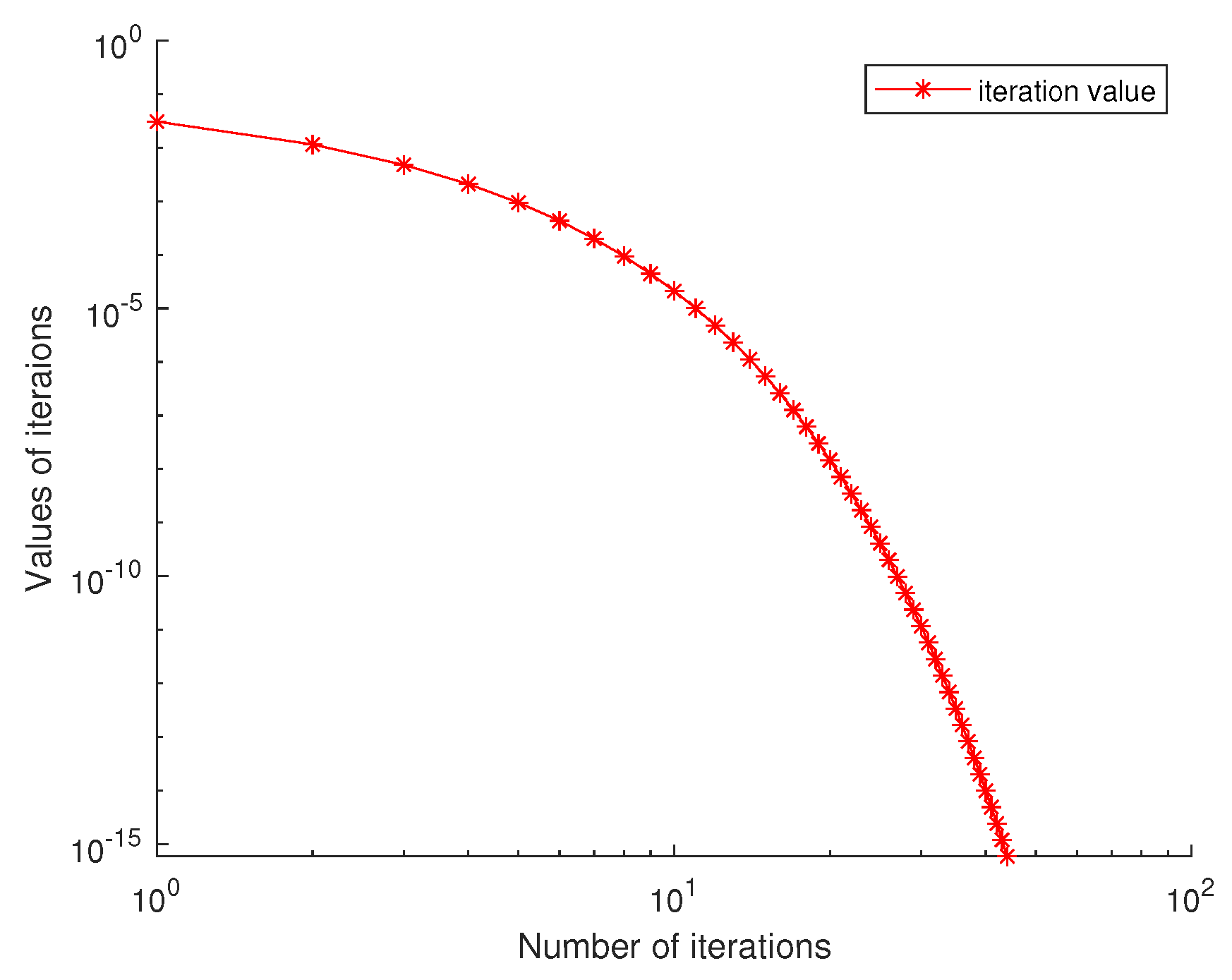
5. Numerical Simulations

In this segment, we furnish a numerical illustration to substantiate the credibility and practicality of our suggested algorithm.

Example 4. 

In ${\mathbb{R}}^2$, we define the functions

$$\begin{array}{cc}\hfill \mathcal{A}(\xi ,\eta )& =\left(\frac{1}{2}\eta log(1+{\xi }^2),-\frac{1}{2}\xi log(1-{\eta }^2)\right)\hfill \\ \hfill \mathcal{B}(\xi ,\eta )& =\left(\frac{1}{2}\eta sin(\xi +\eta ),-\frac{1}{2}\xi sin(\xi +\eta )\right),\hfill \end{array}$$

where $\xi \in \mathbb{R}$. Let $k_n=1+\frac{1}{12n}$, ${\aleph }_n=\frac{1}{3n}$, ${\Re }_n=\frac{1}{2}-\frac{1}{3n}$, and ${\gamma }_n=1-\frac{1}{3n}$ for all $n\in N$. Then we take $t=0.25$, $\mu =3$, $\lambda =2$ and $\mathcal{T}$ and f be defined by $\mathcal{T}(\xi ,\eta )=({\xi }^2,0)$, $f(\xi ,\eta )=(0.25\xi ,0)$. Then, starting with ${\xi }_1=(0.1,0.2)$ in (3), we obtain the following numerical results, as shown in Figure 1 and Figure 2.

6. Conclusions

We first introduced duality mapping and some concepts related to it in a CAT(0) space. We proved some lemmas in a CAT(0) space which are essential for our main result. We considered the problem of the convergence of an iterative algorithm for a system of general variational inequalities and a nonexpansive mapping. Strong convergence theorems are established in the framework of CAT(0) spaces.

References

1. Kinderlehrer, D.; Stampacchia, G. An Introduction to Variational Inequalities and Their Applications; Academic Press: New York, NY, USA, 1980. [Google Scholar]
2. Hartman, P.; Stampacchia, G. On some non-linear elliptic differential-functional equations. Acta Math. 1969, 115, 153–188. [Google Scholar] [CrossRef]
3. Lions, J.L.; Stampacchia, G. Variational inequalities. Commun. Pure Appl. Math. 1967, 20, 493–519. [Google Scholar] [CrossRef]
4. Mancino, O.G.; Stampacchia, G. Convex programming and variational inequalities. J. Optim. Theory Appl. 1972, 9, 3–23. [Google Scholar] [CrossRef]
5. Stampacchia, G. Forms bilineares coercives sur les ensembles convexes. Comptes Rendus Acad. Sci. 1964, 258, 4413–4416. [Google Scholar]
6. Stampacchia, G. Variational inequalities. In theory and applications of monotone operators. In Proceedings of the NATO Advanced Study Institute, Venice, Italy, 1968; Edizioni “Oderisi”; NATO Advanced Study Institute: Gubbio, Italy, 1969; pp. 101–192. [Google Scholar]
7. Facchinei, F.; Pang, J.S. Finite-Dimensional Variational Inequalities and Complimentary Problems; Springer Series in Operations Research; Springer: New York, NY, USA, 2003; Volumes I and II. [Google Scholar]
8. Konnov, I.V. Combined realtion methods for finding equilbrum points and solving related problems. Russ. Math. 1993, 37, 44–51. [Google Scholar]
9. Konnov, I.V. Combined Relaxation Methods for Variatioanl Inequalities; Springer: Berlin/Heidelberg, Germany, 2001. [Google Scholar]
10. Moudafi, A. Viscosity approximation methods for fixed-points problems. J. Math. Anal. Appl. 2000, 241, 46–55. [Google Scholar] [CrossRef]
11. Wangkeeree, R.; Boonkong, U.; Preechasilp, P. Viscosity approximation methods for asymptotically nonexpansive mapping in CAT (0) spaces. Fixed Point Theory Appl. 2015, 2015, 23. [Google Scholar] [CrossRef]
12. Wang, Y.; Pan, C. Viscosity approximation methods for a general variational inequality system and fixed point problems in Banach spaces. Symmetry 2020, 12, 36. [Google Scholar] [CrossRef]
13. Xu, H.K. Viscosity approximation methods for nonexpansive mappings. J. Math. Anal. Appl. 2004, 298, 279–291. [Google Scholar] [CrossRef]
14. Kim, K.S. Convergence theorems of variational inequality for asymptotically nonexpansive nonself mapping in CAT (0) spaces. Mathematics 2019, 7, 1234. [Google Scholar] [CrossRef]
15. Gürsoy, F.; Hacioglu, E.; Karakaya, V.; Milovanović, G.V.; Uddin, I. Variational inequality problem involving multivalued nonexpansive mapping in CAT (0) spaces. Results Math. 2022, 77, 131. [Google Scholar] [CrossRef]
16. Tassaddiq, A.; Kalsoom, A.; Batool, A.; Almutairi, D.K.; Afsheen, S. An Algorithm for Solving Pseudomonotone Variational Inequality Problems in CAT (0) Spaces. Contemp. Math. 2024, 5, 590–601. [Google Scholar] [CrossRef]
17. Gromov, M. Hyperbolic groups. In Essays in Group Theory; Springer: New York, NY, USA, 1987; pp. 75–263. [Google Scholar]
18. Bridson, M.R.; Haefliger, A. Metric Spaces of Non-Positive Curvature; Springer Science and Business Media: Berlin/Heidelberg, Germany, 2013; Volume 319. [Google Scholar]
19. Bruhat, F.; Tits, J. Groupes reductifs sur un corps local. Publ. Math. Inst. Hautes Etudes Sci. 1972, 41, 5–251. [Google Scholar] [CrossRef]
20. Berg, I.D.; Nikolaev, I.G. Quasilinearization and curvature of Aleksandrov spaces. Geom. Dedicata 2008, 133, 195–218. [Google Scholar] [CrossRef]
21. Dhompongsa, S.; Panyanak, B. On -convergence theorems in CAT (0) spaces. Comput. Math. Appl. 2008, 56, 2572–2579. [Google Scholar] [CrossRef]
22. Kakavandi, B.A.; Amini, M. Duality and subdifferential for convex functions on complete CAT (0) metric spaces. Nonlinear Anal. Theory Methods Appl. 2010, 73, 3450–3455. [Google Scholar] [CrossRef]
23. Chaoha, P.; Phon-On, A. A note on fixed point sets in CAT (0) spaces. J. Math. Anal. Appl. 2006, 320, 983–987. [Google Scholar] [CrossRef]
24. Kirk, W.A.; Panyanak, B. A concept of convergence in geodesic spacesmappings. Nonlinear Anal. Theory Methods Appl. 2008, 60, 1345–1355. [Google Scholar]
25. Yao, Y.; Noor, M.A.; Noor, K.I.; Liou, Y.C.; Yaqoob, H. Modified extragradient methods for a system of variational inequalities in Banach spaces. Acta Appl. Math. 2010, 110, 1211–1224. [Google Scholar] [CrossRef]
Figure 1. Real coordinate iteration.
Mathematics 12 02193 g001
Figure 2. Exponential coordinate iteration.
Mathematics 12 02193 g002
Disclaimer/Publisher’s Note: The statements, opinions and data contained in all publications are solely those of the individual author(s) and contributor(s) and not of MDPI and/or the editor(s). MDPI and/or the editor(s) disclaim responsibility for any injury to people or property resulting from any ideas, methods, instructions or products referred to in the content.