An Improved Method for Calculating Wave Velocity Fields in Fractured Rock Based on Wave Propagation Probability

Abstract

Ultrasonic velocity field imaging offers a robust tool for characterizing and analyzing damage and its evolution within fractured rock masses. The combined application of ultrasonic first arrival waves and coda waves can significantly enhance the accuracy and range of velocity field imaging. This manuscript introduces an improved imaging method that integrates the propagation probability distribution of the first arrival and coda waves to calculate the velocity field. The proposed method was applied to the velocity field imaging of a medium with multiple scatterers and varying degrees of fracturing. The overall error and calculation unit error of the proposed method were analyzed, and its improvement in calculation accuracy and applicable scope was verified. Additionally, this method was employed to image the velocity field during the damage process of fractured rock masses. The imaging results were compared against digital speckle patterns to confirm the method’s suitability. Finally, we discussed the impact of measurement errors and sensor missing on the accuracy of the computational outcomes presented in this method. These two situations will affect the calculation results, and the influence of reducing the number of sensors is smaller than that of measuring time shifts with error.

1. Introduction

Fractured rock masses widely exist in underground engineering, and determining their damage distribution and evolution is the key to preventing engineering disasters [1,2]. Wave velocity field imaging based on waveform propagation information in the medium can detect the distribution and evolution of damage inside the medium and is widely used [3,4,5,6]. According to the acoustic wave source [7,8], the wave velocity field imaging algorithm can be divided into two methods: active acoustic wave test imaging and elastic wave information imaging generated by the internal rupture of a rock mass [9,10]. The active acoustic wave test can flexibly adjust the transmitted waveform’s parameter information, transmission time, and frequency [11,12].

At present, studies on the damage detection of rocks [13,14], concrete [15,16], and other materials [17,18] based on wave velocity field imaging have been conducted. Qiangqiang Zheng et al. [19] used a time-varying velocity tomography method based on the Kalman filter system to invert rocks’ wave velocity evolution process under different stresses, considering rock heterogeneity. This new method is used to analyze rock damage evolution and distribution patterns. Bin Liu et al. [20] established a mapping relationship between wave velocity and surrounding rock through wave velocity imaging, providing a new method for advanced geological exploration under complex geological conditions. Jinyoung Yoon [21] et al. used ultrasonic pulses to image the wave velocity field of different layers of concrete and verified it with high-resolution computed tomography. The results showed that the detection results using UPV can be used to determine the flow range of concrete slurry.

Research has demonstrated that ultrasonic coda wave interference (CWI) is exquisitely sensitive to minor alterations within a medium [22,23]. Zotz-Wilson et al. [24] employed the coda wave decorrelation (CWD) method for wave velocity field imaging of the active acoustic wave to scrutinize the damage progression in saturated mudstone. The results showed that the wave velocity of surface coda wave decorrelation in field imaging methods has advantages in initial micro-damage and precision methods. In another study, Chuan Zhang et al. [25] used the coda wave correlation (CWI) method for wave velocity field imaging to closely monitor and assess the interface debonding damage in concrete-rock composites with varying interface roughness. Furthermore, Shilin Qu et al. [26] introduced a novel imaging technique predicated on non-coherent wave interference (NCWI) and incoherent wave interference (INCWI) to visualize cracks that emerge during the three-point bending of concrete beams. The validity and sensitivity of this novel approach were substantiated by comparing the results obtained from microscope observations.

Xiangbo Xu et al. [27] summarized the advantages of ultrasound computed tomography (UCT), emphasizing its high resolution, stability, and low radiation compared with other technologies. Kiran Pandey et al. [28] used the results of direct P wave and coda wave velocity changes to study the evolution of microcracks in different types of granite samples with increasing stress and pressure. The results showed that the CWI method is more sensitive to micro-damage, while the direct P wave interference method is more sensitive to damage along a specific propagation path. Sun Xiangtao et al. [3] pointed out the same problem in monitoring steel bars’ pitting corrosion. Coda waves showed significant sensitivity to subtle pitting corrosion events of steel bars but could not identify severe pitting corrosion. Direct waves show relatively low sensitivity to incipient pitting but vary greatly under severe pitting conditions. They proposed a feature-level data fusion strategy combining coda and direct waves to better identify pitting defects at different stages. Bibo Zhong and Jinying Zhu [29] used ultrasonic coda wave interferometry (CWI). They selected different ultrasonic signal time windows to study the velocity changes of first arrival waves (P), direct shear waves (S), and coda waves in concrete. Their study showed that ultrasonic coda waves have good sensitivity to uniform changes in the velocity of concrete hydration and temperature changes in air entrainment.

The above studies show that ultrasonic coda waves have higher sensitivity when identifying more minor damages [30,31], while ultrasonic direct waves have higher relative accuracy when the damage is more significant [32,33]. Combining ultrasonic coda waves with direct waves for the wave velocity field imaging of rocks will improve detection sensitivity and detection range. Based on the random propagation theory of ultrasound in multi-scatterer media, we propose a wave velocity field imaging method that integrates ultrasonic first-arrival waves and coda waves. This improved approach unites the analysis of ultrasonic direct and coda waves, examining their correlation and the probability distribution of their propagation. It aims to image the wave velocity field of media in a medium containing fractured and multiply scattering bodies, which is subsequently validated within fractured rock masses.

2. Method

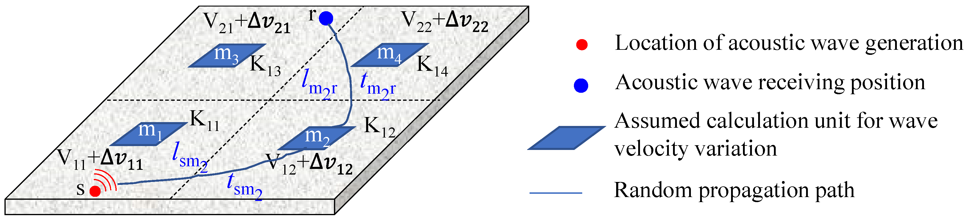
2.1. Probability Calculation of Acoustic Wave Path Propagation Based on Diffusion Theory

Research indicates that within the commonly used MHz frequency range for ultrasonic non-destructive testing, multiple scattering phenomena occur in cementitious materials containing coarse particles [34]. Consequently, the multiple scattering theory can be employed for inversion analysis of medium properties related to coarse particles and defects based on high-frequency acoustic wave testing [35]. In a medium with multiple scattering, we can assume that the energy propagation process of acoustic waves follows a stochastic diffusion process. The diffusion equation describes the average intensity of acoustic wave diffusion in such a multi-scattering medium.

$$\frac{\partial u}{\partial t}=D{\nabla }^{2}u$$

(1)

where u(r, t) is the average intensity, D is the diffusion coefficient, and ${\nabla }^2$ is the two-dimensional Laplace operator.

According to the theory of random diffusion, the average strength at r in an infinite two-dimensional medium can be approximated by the solution of the diffusion equation as follows [36]:

$$P(\mathit{r},t)=\frac{A}{4\pi Dt}\exp \left[\frac{-r^2}{4Dt}\right]$$

(2)

where A is the coefficient.

The solution of the diffusion coefficient can be obtained by fitting the waveforms received by sensors at different positions or by fitting the average intensity of wave propagation with the solution of the diffusion equation [37].

When the acoustic wave propagates in an unbounded media, the propagation path from the acoustic wave emission location to the signal reception location is associated with a corresponding probability. This probability is contingent upon the intensity of wave propagation within the medium. As shown in Figure 1, the schematic diagram below illustrates an unbounded medium, where s represents the acoustic wave generation position, r corresponds to the acoustic wave reception position, and m denotes a region along the path from s to r. Specifically, the distance from s to m is denoted as l_sm, with a corresponding propagation time of t_sm. Similarly, the distance from m to r is l_mr, with a propagation time of t_mr. The total distance from s to r is denoted as l.

Within time t, the probability that a randomly diffused acoustic wave is generated from s and reaches r along a random path through m₂ can be expressed as $P\times dV$. The total energy in this area can be obtained by integrating, as shown below:

$$W(V,t)={\displaystyle {\int }_{v}p(r,t)dV(r)}$$

(3)

The value of W(V,t) equals the probability of a particle arriving at time t during a random propagation. Then, the propagation probability from s to r after taking t time and passing through the m₂ area can be expressed as follows:

$$P(\overrightarrow{s},\overrightarrow{r},t)={\displaystyle {\int }_{v}P(\overrightarrow{s},\overrightarrow{r},{\overrightarrow{m}}_2,t_{s{m}_2},t_{s{m}_2}+t_{m_{2}r})}dv(\overrightarrow{m_2})$$

(4)

Divide the propagating probability from s to r after time t into two parts, and then Equation (2) can be transformed into Equation (3).

$$P(\overrightarrow{s},\overrightarrow{r},t_{sm}+t_{mr})={\displaystyle {\int }_{v}P(\overrightarrow{s},\overrightarrow{m},t_{sm})P(\overrightarrow{m},\overrightarrow{r},t_{mr})}dv(\overrightarrow{m})$$

(5)

By integrating in the time domain, the relationship between the propagation time t and the probability of diffusion intensity can be obtained as follows:

$$t=\frac{1}{P(\overrightarrow{s},\overrightarrow{r},t_{sm}+t_{mr})}{\displaystyle {\int }_v{\displaystyle {\int }_0^{t}P(\overrightarrow{s},\overrightarrow{m},t_{sm})}P(\overrightarrow{m},\overrightarrow{r},t_{mr})}d{t}_{mr}dv(\overrightarrow{m})$$

(6)

Pacheco and Snieder et al. [38] noted that the probability of propagation from s, passing through m within time t, relative to the total probability of propagation from s to r, is defined as the sensitivity kernel K. By substituting into the solution of the stochastic diffusion equation, the sensitivity kernel for two-dimensional space can be expressed as follows:

$$K_{2D}(\mathit{r},t)=\frac{1}{2\pi D}\exp [\frac{-r^2}{2Dt}]K_0[\frac{r^2}{2Dt}]$$

(7)

where K₀ is the zero-order modified Bessel function of the second kind.

The probability distribution of acoustic wave propagation in the medium can be obtained. The distribution of the medium’s wave velocity field can be determined by establishing the relationship between the propagation probability, time shift, and wave velocity.

2.2. Time Shift Solution

According to diffusion theory, the propagation of acoustic waves in a multi-scattering medium can be regarded as the sum of all possible propagation paths. The wave field before and after the medium changes can be represented as follows:

$$\left\{\begin{array}{c}{U}_{ini}(t)={\displaystyle \sum _m}{A}_{m}S\left(t_m\right)\\ U_{dis}(t)={\displaystyle \sum _m}{A}_{m}S(t_m+t_s)\end{array}\right.$$

(8)

where U_ini(t) is the wave field of the media in the initial state; U_dis(t) is the wave field after the medium changes; A_m is the amplitude of the wave propagating along path m; S(t_m) is the corresponding wave train; t_s is the time shift.

As shown in Figure 2, the received waveforms at different detection moments are divided into time windows. Snieder [39] pointed out that the coda wave is the waveform after the wave is scattered three times in the medium. The improved method uses full waveform correlation to calculate the time shift without strictly distinguishing different waveforms. We divide the waveform into a sequence of time intervals by determining the time window length. The time window length is defined as twice the waveform period based on the existing papers [37,39]. At the same time, to avoid the period jump of the time window, the time length of the waveform period is selected as the overlapping part of adjacent time windows. The window cross-correlation method is used to calculate the time shift of each time window. By assessing the waveform correlation across different time windows, the time shift data corresponding to the variation in the wave velocity field can be determined [40].

$$R^{(t_{w1},t_{w2})}(t_s)=\frac{{\displaystyle {\int }_{t_{w1}}^{t_{w2}}{\displaystyle \sum _T{A}_T(t^{\prime })}{\displaystyle \sum _T{A}_T(t^{\prime }-{\tau }_T+t_s)}d{t}^{\prime }}}{\sqrt{{\displaystyle {\int }_{t_{w1}}^{t_{w2}}{\displaystyle \sum _T{A}_T^2(t^{\prime })}d{t}^{\prime }}}\sqrt{{\displaystyle {\int }_{t_{w1}}^{t_{w2}}{\displaystyle \sum _T{A}_T^2(t^{\prime }-{\tau }_T+t_s)}d{t}^{\prime }}}}$$

(9)

where R^(tw1,tw2)(t_s) is the correlation coefficient; (t_w1, t_w2) is the time window; T is a combination of random paths; A_T(t) is the corresponding waveform.

2.3. Wave Velocity Field Calculation

In a multi-scatterer medium, the wave velocity changes as the propagation time changes when the medium changes. The relationship between time shift and wave propagation intensity probability can be expressed as follows:

$$t+\Delta t=\frac{1}{P(\overrightarrow{s},\overrightarrow{r},t_{sm}+t_{mr})}{\displaystyle {\int }_v{\displaystyle {\int }_0^t\frac{V+\Delta V}{V}P(\overrightarrow{s},\overrightarrow{m},t_{sm})}P(\overrightarrow{m},\overrightarrow{r},t_{mr})}d{t}_{mr}dv(\overrightarrow{m})$$

(10)

After the deconvolution of the probability distribution of wave propagation into Equation (10), the following relationship can be obtained:

$$\Delta \overline{t}=\frac{1}{2\pi D}{\displaystyle {\int }_v\exp [\frac{-r^2}{2Dt}]K_0[\frac{r^2}{2Dt}]\frac{\Delta l}{L}}(\mathit{m})dV(\mathit{m})$$

(11)

Taking Figure 1 as an example, the relationship between time shift and wave velocity change can be expressed as follows:

$$\left[\begin{array}{l}{t}_1\\ t_2\\ \cdots \\ t_m\end{array}\right]=\left[\begin{array}{cccc}\Delta s{K}_{11}& \Delta s{K}_{12}& \cdots & \Delta s{K}_{1n}\\ \Delta s{K}_{21}& \Delta s{K}_{22}& \cdots & \Delta s{K}_{2n}\\ \cdots & \cdots & \cdots & \cdots \\ \Delta s{K}_{m1}& \Delta s{K}_{m2}& \cdots & \Delta s{K}_{mn}\end{array}\right]\left[\begin{array}{c}{V}_1\\ V_2\\ \cdots \\ V_n\end{array}\right]$$

(12)

where t_i (i = [1, m]) is the time shift of the waveform received by the deployed sensors; m is the number of time windows; K is the sensitivity kernel; V_n is the wave velocity variation to be solved; and n is the number of wave velocity elements to be solved.

G is the mapping between time shift and wave velocity variation. Its calculation formula is as follows:

$$G=K\Delta s=\left[\begin{array}{cccc}\Delta s{K}_{11}& \Delta s{K}_{12}& \cdots & \Delta s{K}_{1n}\\ \Delta s{K}_{21}& \Delta s{K}_{22}& \cdots & \Delta s{K}_{2n}\\ \cdots & \cdots & \cdots & \cdots \\ \Delta s{K}_{m1}& \Delta s{K}_{m2}& \cdots & \Delta s{K}_{mn}\end{array}\right]$$

(13)

C_t is the diagonal covariance matrix of the measured data. This matrix’s elements are the standard deviation of the time shift change calculated based on the correlation of the full waveform. Its calculation formula is as follows:

$$C_{tii}=\frac{\sqrt{1-R_i^2}}{2R_i}\sqrt{\frac{6\sqrt{\frac{\pi }{2}}T}{{\omega }_c^2(t_2^3-t_1^3)}}$$

(14)

where R_i is the correlation coefficient of the corresponding time window; T is the main period of the waveform; ${\omega }_c=2\pi f_c$; t₁ and t₂ are the start and end times of the time window, respectively.

C_v represents the deviation between the actual model and the prior information. Its function is to reduce the uncertainty of the equation to be solved. It is a diagonal covariance matrix, and the expression is as follows:

$$C_{vii}=\left(st{d}_m\frac{L_0}{L_c}\right)\exp (-\frac{\left|X_i-X_j\right|}{L_c})$$

(15)

where std_m is the standard deviation of the velocity field matrix V to be solved; L₀ is the distance between sensitive nuclei; $\left|X_i-X_j\right|$ is the distance between two grid elements i and j; L_c is obtained by regularization fitting V and T using the L-curve method. The calculation process is shown in Figure 3.

3. Numerical and Experimental Verification

3.1. Numerical Verification

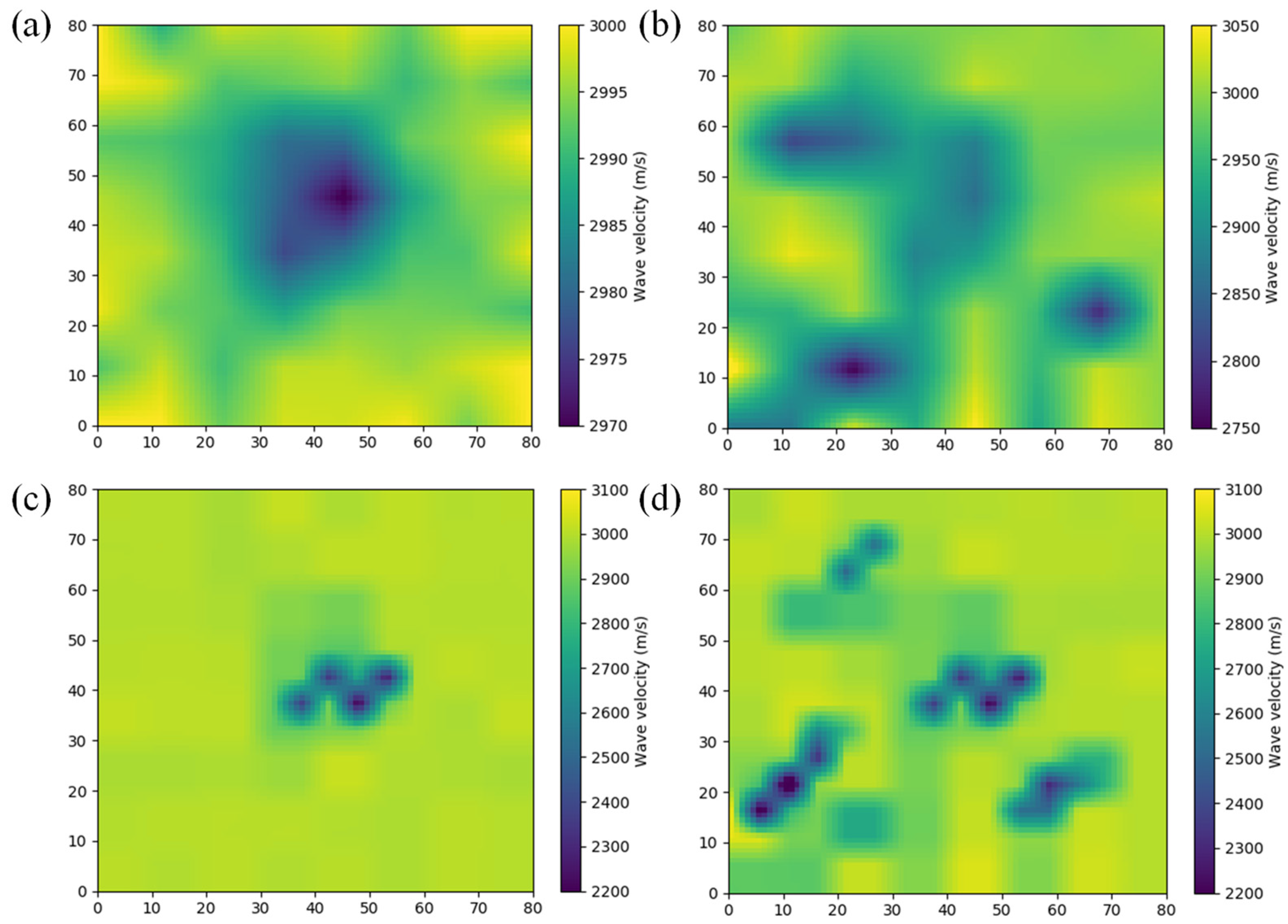
3.1.1. Numerical Model

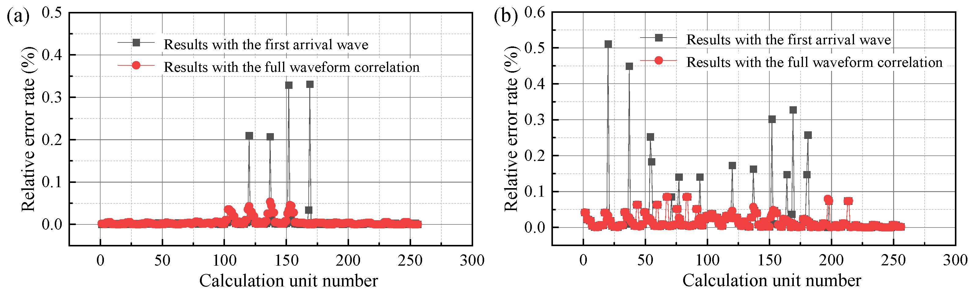
This manuscript validates the proposed algorithm’s accuracy and applicability through numerical simulations and indoor experiments. As depicted in Figure 4, the numerical simulation model utilizes finite element analysis to generate a multi-scattering medium with dimensions of 100 m × 100 m × 1 m as the initial medium model. The model is based on a linear elastic framework, with boundary conditions representing a free boundary with reflective waves. The model parameters are chosen based on the typical material properties of rock. Specifically, for sandstone, the bulk density ranges from 2000 kg/m³ to 2600 kg/m³, Young’s modulus spans from 9.8 GPa to 98 GPa, and the Poisson’s ratio varies between 0.2 and 0.3. The numerical model incorporates these relevant parameters, and the relationship between these parameters and the medium’s wave velocity is defined according to Equations (1) through (6). The elastic modulus of the model is set to 25 GPa, and the Poisson’s ratio is fixed at 0.3.

Different wave velocities of the medium can be obtained by varying the density. The initial medium is divided into 10,000 cells, with each cell’s initial wave velocity randomly set to 3200 ± 20 m/s. Generate two and six cracks on the initial medium, with each crack’s wave velocity set to 300 m/s per cell. The center position coordinates, inclination angle, and length of the cracks are shown in

Table 1. Crack parameters.

Crack’s Number	Coordinate of the Crack Center Point		Crack Length (m)	Crack Inclination Angle (°)
	X	Y
1	40	40	10	30
2	50	40	11	53
3	10	20	13	60
4	25	65	8	34
5	18	30	7	63
6	57	20	8	78

. The actual wave velocity of the medium is determined by averaging the wave velocities of all cells within the detection area of the model. The resulting initial medium has a wave velocity of 3186 m/s. The overall actual wave velocities of the medium corresponding to Figure 4b and Figure 4c are 3121 m/s and 3046 m/s, respectively. Around the monitoring area, 12 sensors capable of emitting and receiving acoustic waves are placed. These sensors take turns emitting vibrational waves, and the remaining sensors receive the acoustic waves. The coordinates of the monitoring sensors are shown in

Table 2. Coordinates of the sensors.

	Sensors’ Number
	1	2	3	4	5	6	7	8	9	10	11	12
X	10	40	60	80	80	80	70	40	20	0	0	0
Y	0	0	0	10	40	60	80	80	80	70	40	20

.

For media with different numbers of cracks, ensure that the position and waveform of the transmitted waveform remain unchanged, and calculate the change in the wave velocity field of the medium based on the received waveform information. Twelve sensors take turns emitting acoustic waves, and the remaining sensors receive the acoustic waves. The emitted acoustic wave is a 150 kHz sine wave. When the acoustic wave is emitted from sensor 2 and propagates to sensor 8, the distribution of the wave velocity field in the medium is shown in Figure 4d–f.

3.1.2. Results

When sensor 1 is the acoustic source, the remaining 11 sensors receive the acoustic signals. Nine valid rays are left after excluding the ineffective rays on the same side as sensor 1. Similarly, we removed same-sided and duplicate rays for other monitoring points, resulting in the corresponding number of effective rays, as shown in

Table 3. Effective ray number corresponding to different sensors.

Sensor number	1	2	3	4	5	6	7	8	9	10	11	12
Effective ray number	9	9	9	6	6	6	3	3	3	0	0	0

.

For any medium model, 132 waveform data are used to invert and calculate the wave velocity field.

The wave velocity field of the fractured medium was calculated using the proposed method, and the results are shown in Figure 5. Figure 5a,b are the wave velocity field results calculated using only the first arrival wave information. Figure 5c,d are the wave velocity field results calculated by the proposed method. When the number of cracks in the model is two, the error percentage of the improved method is 0.55%, and the error percentage of the calculation using the first arrival wave is 0.65%. When the number of cracks in the model is four, the error percentage of the improved method is 1.62%, and the error percentage of the calculation using the first arrival wave is 2.71%. The calculation results of the proposed method are highly accurate.

The calculation unit errors of different crack models are shown in Figure 6. Figure 6a shows the error rate of the calculation unit with two cracks, and Figure 6b shows the error rate of the calculation unit with four cracks. Since the wave velocity at the crack is much lower than the surrounding wave velocity, the calculation unit error at the crack is relatively high. This is especially true when only the first arrival wave travel time is used.

3.2. Experimental Verification

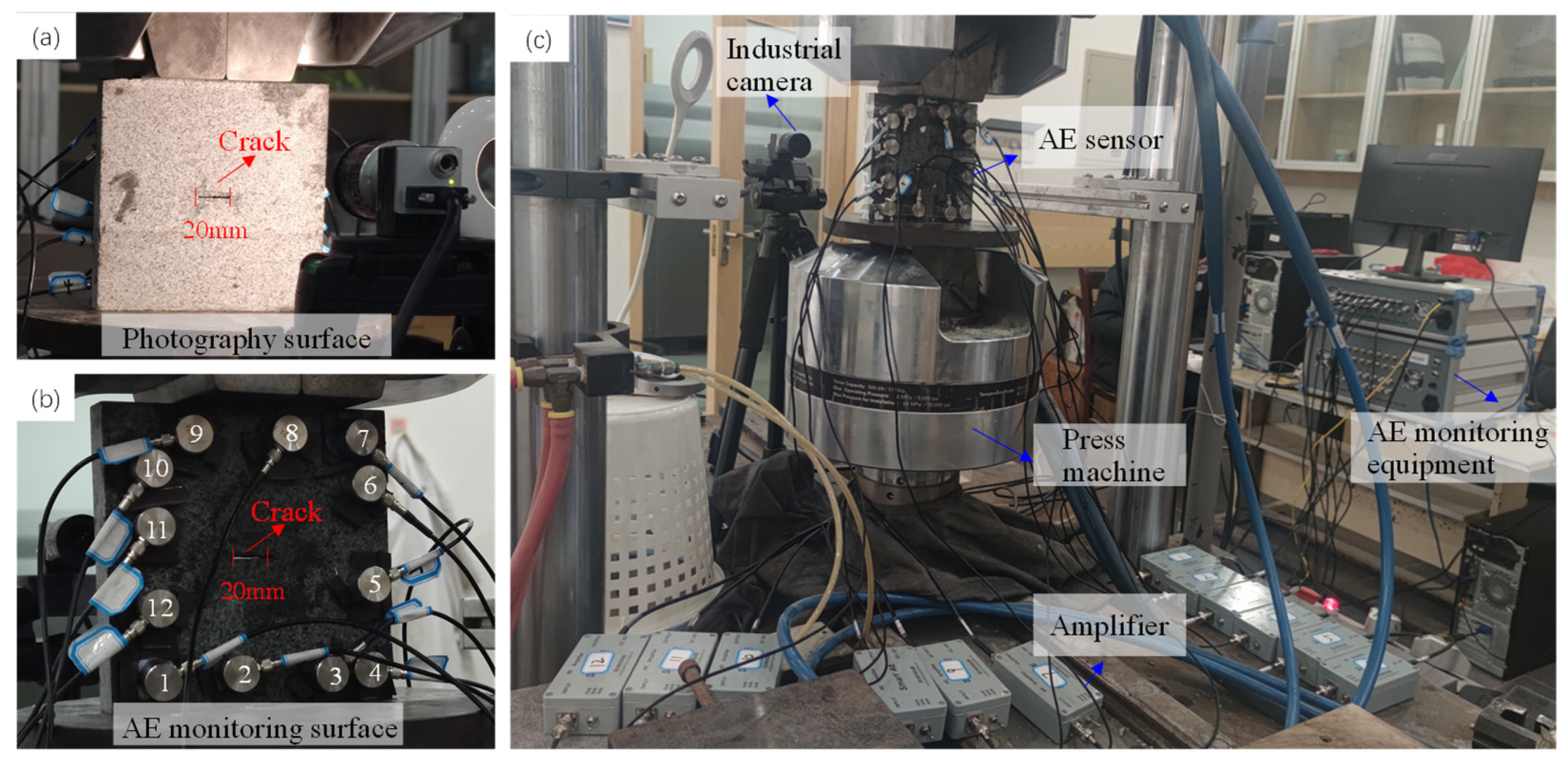
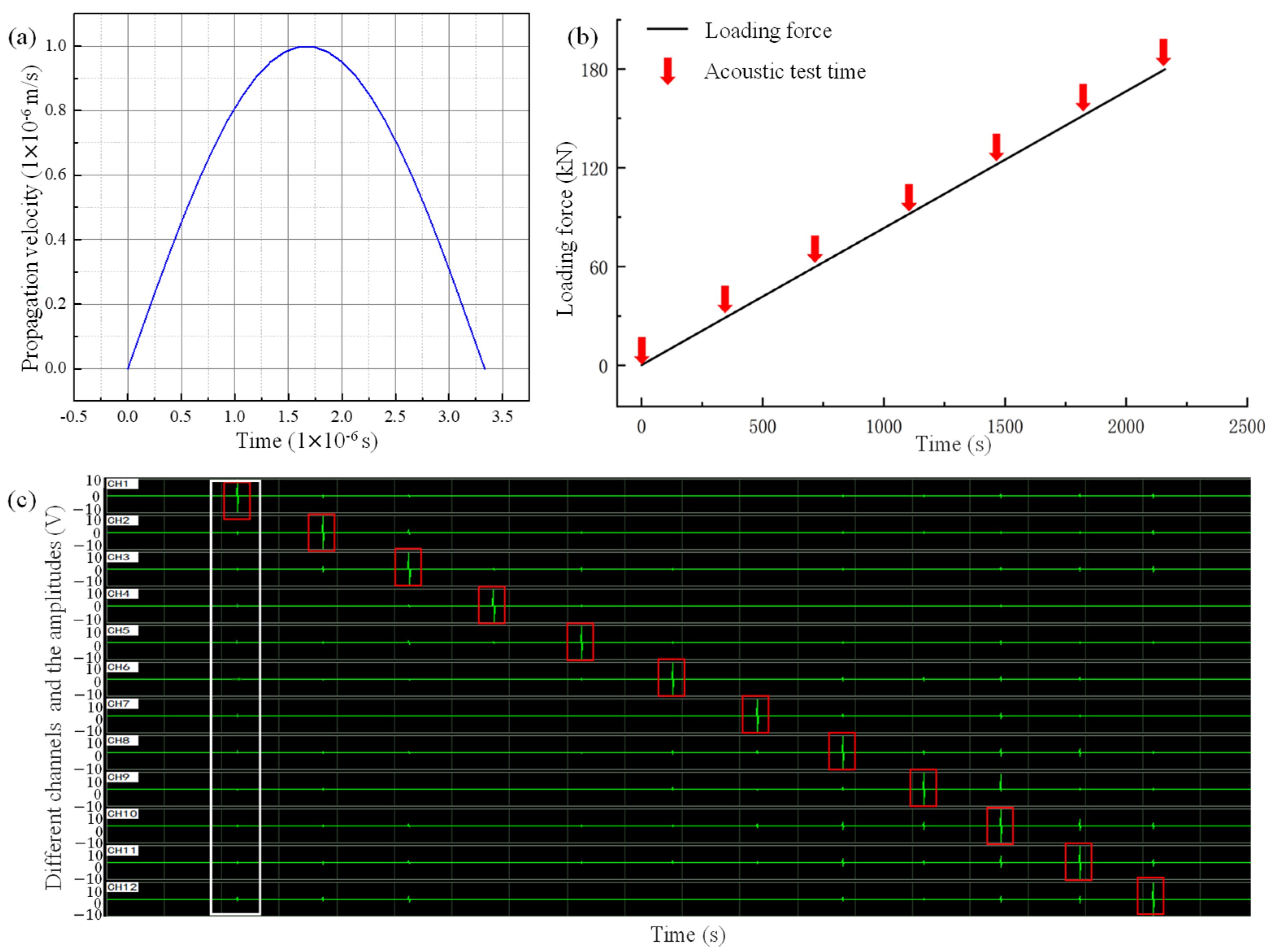
3.2.1. Experiment Process

The material employed in the experimental verification is a granite slab specimen with dimensions of 200 mm × 200 mm. Centrally located within the specimen is a 20 mm × 1 mm crack, as shown in Figure 7a. Figure 7b is the AE monitoring surface of the granite slab specimen. Axial pressure was applied to the specimen via a press to induce damage, with the utilized press apparatus illustrated in Figure 7c.

An industrial camera took pictures on one side of the specimen, and digital speckle technology evaluated the damage during loading. On the opposite side, 12 acoustic emission sensors emitted acoustic waves during loading. The emitted acoustic waveform is shown in Figure 8a, and the variation process of the loading force of the specimen with time is shown in Figure 8b. An acoustic test was carried out before the start of the experiment, followed by additional tests every 30 kN of load applied. The last acoustic wave test was carried out after the obvious crack appeared, and seven acoustic wave tests were carried out. The arrows in Figure 8b show each acoustic test moment. Figure 8c shows a thumbnail of the 12 sensors taking turns emitting acoustic waves and receiving waveforms. The red squares in the figure represent the sensors that emit acoustic waves. The white squares represent a thumbnail of an acoustic test’s transmitted and received waveforms.

In the experimental process, the diffusion coefficient is obtained by fitting the average intensity of wave propagation with the solution of the diffusion equation, as shown in Figure 9.

3.2.2. Results

The proposed method calculates the wave velocity field imaging at different times and compares it with the digital speckle results. The calculation is shown in Figure 10. Figure 10a shows the results obtained by digital speckle. Figure 9b is the wave velocity calculated by the improved method. The improved method combines the advantages of first wave arrival and coda wave, can sense the initial damage of the sample, and improves the sensitivity of wave speed change perception.

4. Discussion

4.1. The Influence of the AE Sensor Missing on the Calculation Results

This section selects the multi-scattering medium model with two cracks used in Section 3 to analyze the influencing factors.

Since the acoustic emission sensor fell off due to the damage and deformation of the monitoring sample, the impact of the reduction in the number of sensors on the calculation results was analyzed. Additionally, since there were errors in the measurement process, the effect of different levels of measurement errors on the calculation results was analyzed. The relative error rate, average error rate, and correlation coefficient of the calculation unit were used to evaluate the accuracy of the calculation results.

The relative error rate and average error rate were calculated as follows:

$$\left\{\begin{array}{c}{\delta }_i=\frac{v_i-v_i^0}{v_i^0}\\ \overline{\delta }=\frac{1}{n}{\displaystyle \sum _{i=1}^n\left|{\delta }_i\right|}\end{array}\right.$$

(16)

where v_i is the wave velocity of the ith calculation unit, $v_i^0$ is the actual wave velocity, n is the number of calculation units, and ${\delta }_i$ is the calculation error of the ith calculation unit.

The correlation coefficient of the calculation unit was calculated as follows:

$$R=\frac{{\displaystyle \sum _{j=1}^n(v_j-\overline{v})(v_0-{\overline{v}}_0)}}{\sqrt{{\displaystyle \sum _{j=1}^n{(v_j-\overline{v})}^2}}\sqrt{{\displaystyle \sum _{j=1}^n{(v_0-{\overline{v}}_0)}^2}}}$$

(17)

where v_j is the wave velocity of the ith calculation unit, $\overline{v}$ is the average value of velocity, $v_0$ is the tactualwave velocity, and ${\overline{v}}_0$ is the average of the actual wave velocity.

The deformation during the damage process of the specimen caused the sensor to fall off, affecting the wave velocity field imaging results. The wave velocity field imaging errors of the two crack models in Section 3.1 were calculated when the number of missing sensors was two, four, six, and eight. The missing sensor numbers were 1, 2, 4, 5, 7, 8, 10, and 11.

Figure 11 shows the error calculation results. Figure 11a shows the effect of sensor loss on the overall error rate of the calculation results. The average error rate and the correlation coefficient with the accurate result were used for evaluation. Figure 11b shows the error rate of each calculation unit. When the number of missing sensors is less than four, the error rate is relatively small, and the correlation coefficient is relatively high. When the number of disappeared paths exceeds six, the overall error rate and the calculation unit error at the crack are both significant.

4.2. The Influence of the Wave Path Measurement Error on Calculation Results

The error rates of 1%, 2%, 3%, and 4% were added to the propagation path time-shift measurement error. The velocity field inversion results under different error rates were calculated respectively. The influence of the propagation path time-shift measurement error on the accuracy of the calculation results was analyzed based on the overall average error rate and the calculation unit error rate.

Figure 12 illustrates the impact of the arrival time error on the calculation results. Figure 12a shows the average error rate and correlation coefficient with the actual result at different measurement error rate levels. Figure 12b shows the calculation unit error rate at different measurement error rate levels. The results show that the measurement error rate dramatically influences the calculation result. When the error rate is greater than 1%, the correlation coefficient with the actual result is less than 0.5, and the average error rate is greater than 2%. At the same time, the calculation unit error rate of the defect position is significant.

Compared with the path error, the impact of the missing sensor is smaller than the case where the path has an error. By comparing Figure 6, Figure 11 and Figure 12, it can be observed that the measurement errors and missing sensors will increase the calculation error at the defect. Therefore, the impact of the error should be minimized as much as possible in the application.

5. Conclusions

This manuscript proposed an imaging method for the wave velocity field of fractured rock masses based on the probability distribution of wave propagation. The method integrates the advantages of ultrasonic direct waves and coda waves in damage detection. The time shift in the time window is calculated using waveform correlation. The relationship between the time shift at different time windows and the wave velocity field variation is established based on the probability distribution of wave propagation in a multi-scattering medium. The accurate wave velocity field is obtained by correcting the initial wave velocity field. The method has been verified in multi-scattering media with different fractures and applied to imaging the wave velocity field during the damage evolution process of fractured rocks. The influencing factors of the proposed method have been discussed. The main conclusions are as follows:

(1)

Based on the stochastic theory of wave propagation in a multi-scattering medium, an imaging method for the wave velocity field based on the probability distribution of wave propagation is proposed. This method combines the advantages of the time shift of the first arrival wave and the coda wave, which not only allows for the determination of the wave velocity field distribution in the medium with existing damage but also enhances the sensitivity of wave velocity field evolution perception in the medium.

(2)

Numerical models of fractures with different characteristics were established, and the wave velocity field of models with different fractures was inverted using the proposed method. The relative error rate between the computational units solved by the proposed method and the first arrival wave was analyzed, and the results showed that the computational accuracy of the proposed method has been relatively improved.

(3)

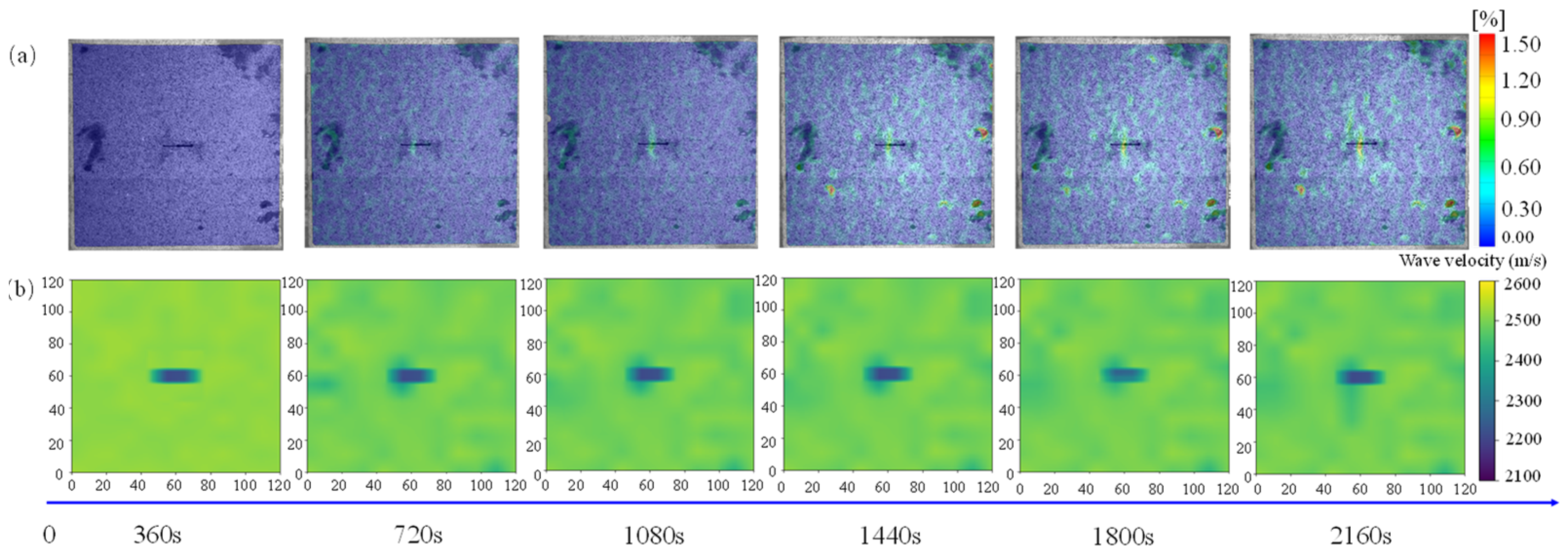
An experiment with a rock slab containing fractures was conducted, and the evolution of the wave velocity field during the loading process was calculated using the proposed method. The results were compared and analyzed with digital speckle results, indicating that the proposed method can accurately obtain the distribution of the wave velocity field during the damage evolution process of rocks.

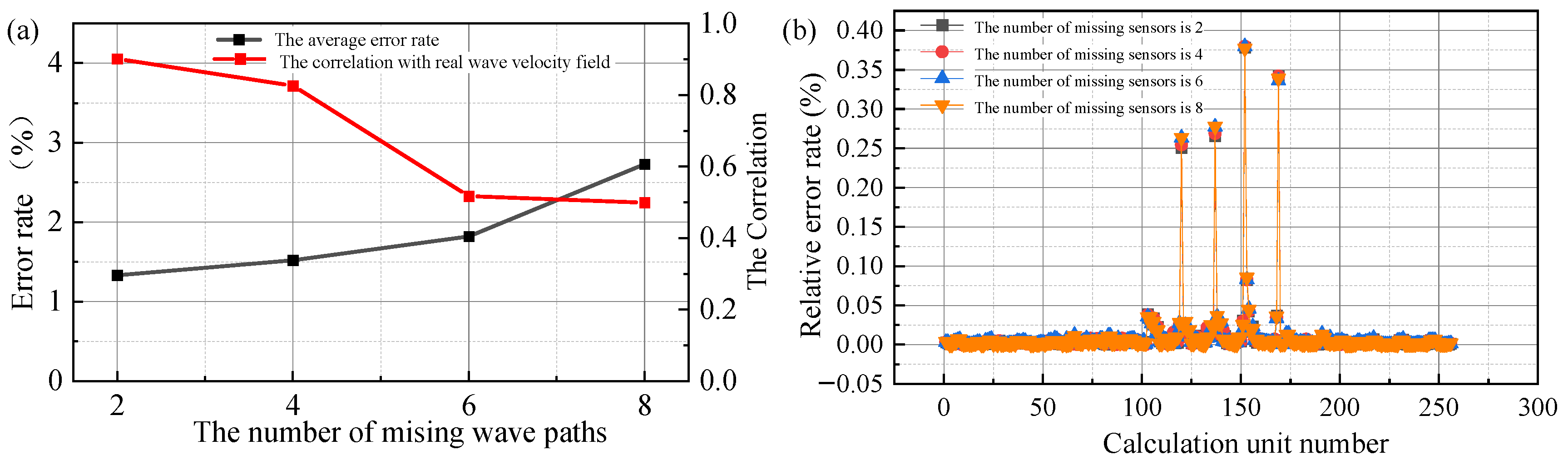
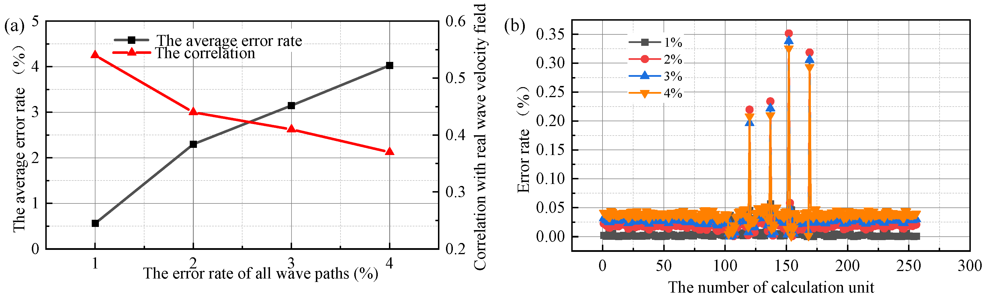
(4)

Considering the loss of sensors and the error of measured time shift data caused by medium deformation damage, the influence of reducing the number of sensors by two, four, six, and eight and the error level of propagation path measured time shift by 1%, 2%, 3% and 4% on the calculation results are analyzed respectively. The results show that these two situations will affect the calculation results, and the influence of reducing the number of sensors is smaller than that of measuring time shifts with error.

References

1. Lu, J.; Zhou, Z.; Chen, X.; Wang, P.; Rui, Y.; Cai, X. Experimental investigation on mode I fracture characteristics of rock-concrete interface at different ages. Constr. Build. Mater. 2022, 349, 128735. [Google Scholar] [CrossRef]
2. Tan, L.; Zhou, Z.; Cai, X.; Rui, Y. Analysis of mechanical behaviour and fracture interaction of multi-hole rock mass with DIC measurement. Measurement 2022, 191, 110794. [Google Scholar] [CrossRef]
3. Sun, X.; Zhang, M.; Gao, W.; Guo, C.; Kong, Q. A novel method for steel bar all-stage pitting corrosion monitoring using the feature-level fusion of ultrasonic direct waves and coda waves. Struct. Health Monit. 2023, 22, 714–729. [Google Scholar] [CrossRef]
4. Zhou, J.; Liu, L.; Zhao, Y.; Zhu, M.; Wang, R.; Zhuang, D. An Improved Rock Damage Characterization Method Based on the Shortest Travel Time Optimization with Active Acoustic Testing. Mathematics 2024, 12, 161. [Google Scholar] [CrossRef]
5. Shokouhi, P.; Rivière, J.; Lake, C.R.; Le Bas, P.-Y.; Ulrich, T.J. Dynamic acousto-elastic testing of concrete with a coda-wave probe: Comparison with standard linear and nonlinear ultrasonic techniques. Ultrasonics 2017, 81, 59–65. [Google Scholar] [CrossRef] [PubMed]
6. Babaei, M.; Kiarasi, F.; Marashi, S.M.H.; Ebadati, M.; Masoumi, F.; Asemi, K. Stress wave propagation and natural frequency analysis of functionally graded graphene platelet-reinforced porous joined conical–cylindrical–conical shell. Waves Random Complex Media 2021, 1–33. [Google Scholar] [CrossRef]
7. Dong, L.; Cao, H.; Hu, Q.; Zhang, S.; Zhang, X. Error distribution and influencing factors of acoustic emission source location for sensor rectangular network. Measurement 2024, 225, 113983. [Google Scholar] [CrossRef]
8. Dong, L.; Chen, Y.; Sun, D.; Zhang, Y.; Deng, S. Implications for identification of principal stress directions from acoustic emission characteristics of granite under biaxial compression experiments. J. Rock Mech. Geotech. Eng. 2023, 15, 852–863. [Google Scholar] [CrossRef]
9. Zhang, G.; Wu, S.; Zhang, S.; Guo, P. P-wave velocity tomography and acoustic emission characteristics of sandstone under uniaxial compression. Rock Soil. Mech. 2023, 44, 9. [Google Scholar] [CrossRef]
10. Lan, M.; Tang, Y.; Ma, J.; Liu, Z. Cooperative acoustic emission locating with velocity tomography in true triaxial experiment. Eng. Fract. Mech. 2023, 292, 109633. [Google Scholar] [CrossRef]
11. Liu, D.; Cao, K.; Tang, Y.; Zhong, A.; Jian, Y.; Gong, C.; Meng, X. Ultrasonic and X-CT measurement methods for concrete deterioration of segmental lining under wetting-drying cycles and sulfate attack. Measurement 2022, 204, 111983. [Google Scholar] [CrossRef]
12. Wojtczak, E.; Rucka, M.; Skarżyński, Ł. Monitoring the fracture process of concrete during splitting using integrated ultrasonic coda wave interferometry, digital image correlation and X-ray micro-computed tomography. NDT E Int. 2022, 126, 102591. [Google Scholar] [CrossRef]
13. Zhang, Y.; Yao, X.; Liang, P.; Wang, K.; Sun, L.; Tian, B.; Liu, X.; Wang, S. Fracture evolution and localization effect of damage in rock based on wave velocity imaging technology. J. Cent. South Univ. 2021, 28, 2752–2769. [Google Scholar] [CrossRef]
14. Zhang, W.; Sun, Q.; Zhang, Y.; Xue, L.; Kong, F. Porosity and wave velocity evolution of granite after high-temperature treatment: A review. Environ. Earth Sci. 2018, 77, 350. [Google Scholar] [CrossRef]
15. Varamashvili, N.D.; Asanidze, B.Z.; Jakhutashvili, M.N. Ultrasonic Tomography and Pulse Velocity for Nondestructive Testing of Concrete Structures. J. Georgian Geophys. Soc. 2020, 23, 14–20. [Google Scholar] [CrossRef]
16. Krauß, M.; Hariri, K. Determination of initial degree of hydration for improvement of early-age properties of concrete using ultrasonic wave propagation. Cem. Concr. Compos. 2006, 28, 299–306. [Google Scholar] [CrossRef]
17. Farin, M.; Moulin, E.; Chehami, L.; Benmeddour, F.; Nicard, C.; Campistron, P.; Bréhault, O.; Dupont, L. Monitoring saltwater corrosion of steel using ultrasonic coda wave interferometry with temperature control. Ultrasonics 2022, 124, 106753. [Google Scholar] [CrossRef] [PubMed]
18. Liu, Y.; Ding, W.; Dong, P.; Okude, N.; Asaue, H.; Shiotani, T. Identification of hydration stages: An innovative study of ultrasonic coda waves using integrated sensing element (ISE). Constr. Build. Mater. 2023, 401, 132764. [Google Scholar] [CrossRef]
19. Zheng, Q.; Qian, J.; Zhang, H.; Chen, Y.; Zhang, S. Velocity tomography of cross-sectional damage evolution along rock longitudinal direction under uniaxial loading. Tunn. Undergr. Space Technol. 2024, 143, 105503. [Google Scholar] [CrossRef]
20. Liu, B.; Wang, J.; Yang, S.; Xu, X.; Ren, Y. Forward prediction for tunnel geology and classification of surrounding rock based on seismic wave velocity layered tomography. J. Rock Mech. Geotech. Eng. 2023, 15, 179–190. [Google Scholar] [CrossRef]
21. Yoon, J.; Kim, H.; Shin, S.W.; Sim, S.-H. Rheology-based determination of injectable grout fluidity for preplaced aggregate concrete using ultrasonic tomography. Constr. Build. Mater. 2020, 260, 120447. [Google Scholar] [CrossRef]
22. Shan, S.; Liu, Z.; Cheng, L.; Pan, Y. Metamaterial-enhanced coda wave interferometry with customized artificial frequency-space boundaries for the detection of weak structural damage. Mech. Syst. Signal Process. 2022, 174, 109131. [Google Scholar] [CrossRef]
23. Cheng, W.; Fan, Z.; Tan, K.H. Characterisation of corrosion-induced crack in concrete using ultrasonic diffuse coda wave. Ultrasonics 2023, 128, 106883. [Google Scholar] [CrossRef] [PubMed]
24. Zotz-Wilson, R.; Douma, L.A.N.R.; Sarout, J.; Dautriat, J.; Dewhurst, D.; Barnhoorn, A. Ultrasonic Imaging of the Onset and Growth of Fractures Within Partially Saturated Whitby Mudstone Using Coda Wave Decorrelation Inversion. J. Geophys. Res. Solid Earth 2020, 125, e2020JB020042. [Google Scholar] [CrossRef]
25. Zhang, C.; Yan, Q.; Zhang, Y.; Liao, X.; Zhong, H. Intelligent monitoring of concrete-rock interface debonding via ultrasonic measurement integrated with convolutional neural network. Constr. Build. Mater. 2023, 400, 131865. [Google Scholar] [CrossRef]
26. Qu, S.; Hilloulin, B.; Saliba, J.; Sbartaï, M.; Abraham, O.; Tournat, V. Imaging concrete cracks using Nonlinear Coda Wave Interferometry (INCWI). Constr. Build. Mater. 2023, 391, 131772. [Google Scholar] [CrossRef]
27. Xu, X.; Ran, B.; Jiang, N.; Xu, L.; Huan, P.; Zhang, X.; Li, Z. A systematic review of ultrasonic techniques for defects detection in construction and building materials. Measurement 2024, 226, 114181. [Google Scholar] [CrossRef]
28. Pandey, K.; Taira, T.; Dresen, G.; Goebel, T.H. Inferring damage state and evolution with increasing stress using direct and coda wave velocity measurements in faulted and intact granite samples. Geophys. J. Int. 2023, 235, 2846–2861. [Google Scholar] [CrossRef]
29. Zhong, B.; Zhu, J. Applications of Stretching Technique and Time Window Effects on Ultrasonic Velocity Monitoring in Concrete. Appl. Sci. 2022, 12, 7130. [Google Scholar] [CrossRef]
30. Planès, T.; Larose, E. A review of ultrasonic Coda Wave Interferometry in concrete. Cem. Concr. Res. 2013, 53, 248–255. [Google Scholar] [CrossRef]
31. Hilloulin, B.; Zhang, Y.; Abraham, O.; Loukili, A.; Grondin, F.; Durand, O.; Tournat, V. Small crack detection in cementitious materials using nonlinear coda wave modulation. NDT E Int. 2014, 68, 98–104. [Google Scholar] [CrossRef]
32. Marcantonio, V.; Monarca, D.; Colantoni, A.; Cecchini, M. Ultrasonic waves for materials evaluation in fatigue, thermal and corrosion damage: A review. Mech. Syst. Signal Process. 2019, 120, 32–42. [Google Scholar] [CrossRef]
33. Liu, Z.; Yao, Q.; Kong, B.; Yin, J. Macro-micro mechanical properties of building sandstone under different thermal damage conditions and thermal stability evaluation using acoustic emission technology. Constr. Build. Mater. 2020, 246, 118485. [Google Scholar] [CrossRef]
34. Tourin, A.; Derode, A.; Peyre, A.; Fink, M. Transport parameters for an ultrasonic pulsed wave propagating in a multiple scattering medium. J. Acoust. Soc. Am. 2000, 108, 503–512. [Google Scholar] [CrossRef] [PubMed]
35. Biwa, S.; Yamamoto, S.; Kobayashi, F.; Ohno, N. Computational multiple scattering analysis for shear wave propagation in unidirectional composites. Int. J. Solids Struct. 2004, 41, 435–457. [Google Scholar] [CrossRef]
36. Margerin, L.; Planès, T.; Mayor, J.; Calvet, M. Sensitivity kernels for coda-wave interferometry and scattering tomography: Theory and numerical evaluation in two-dimensional anisotropically scattering media. Geophys. J. Int. 2016, 204, 650–666. [Google Scholar] [CrossRef]
37. Xie, F.; Ren, Y.; Zhou, Y.; Larose, E.; Baillet, L. Monitoring Local Changes in Granite Rock Under Biaxial Test: A Spatiotemporal Imaging Application With Diffuse Waves. J. Geophys. Res. Solid Earth 2018, 123, 2214–2227. [Google Scholar] [CrossRef]
38. Pacheco, C.; Snieder, R. Time-lapse travel time change of multiply scattered acoustic waves. J. Acoust. Soc. Am. 2005, 118, 1300–1310. [Google Scholar] [CrossRef]
39. Snieder, R. Coda Wave Interferometry for Estimating Nonlinear Behavior in Seismic Velocity. Science 2002, 295, 2253–2255. [Google Scholar] [CrossRef]
40. Zhou, J.; Zhou, Z.; Zhao, Y.; Cai, X. Global Wave Velocity Change Measurement of Rock Material by Full-Waveform Correlation. Sensors 2021, 21, 7429. [Google Scholar] [CrossRef]
Figure 1. Acoustic wave propagation model.
Mathematics 12 02177 g001
Figure 2. The arrival wave and time window. (a) is the first arrival wave, coda wave, and noise wave. (b) is the enlarged image of the first arrival wave. (c) is the time window.
Mathematics 12 02177 g002
Figure 3. The calculation process of the improved method.
Mathematics 12 02177 g003
Figure 4. (ac) are the multi-scatterer medium model with cracks. (df) are the wave field intensity diagram of acoustic waves propagating to the sensor.
Mathematics 12 02177 g004
Figure 5. Results with different methods. (a,b) are the results calculated with the first arrival wave. (c,d) are the results calculated using the improved method.
Mathematics 12 02177 g005
Figure 6. The error rate of the calculation unit. (a,b) are the relative error rates of the calculation unit when there are two and four cracks in the multi-scatterer model, respectively.
Mathematics 12 02177 g006
Figure 7. Experimental materials and equipment. (a,b) are the photographic surface and acoustic emission monitoring surface of the granite slab specimen, respectively. 1–12 in the (b) are the number of AE sensors. (c) is the experimental system diagram.
Mathematics 12 02177 g007
Figure 8. Transmit waveform, transmit time, and receive waveform. (a) is the emitted acoustic waveform. (b) is the variation process of the loading force of the specimen with time. (c) is the waveform of each channel.
Mathematics 12 02177 g008
Figure 9. The diffusion coefficient solution process. (a) is the waveform and waveform envelope. (b) is the curve fitting of the waveform.
Mathematics 12 02177 g009
Figure 10. Digital speckle results and wave velocity field imaging results. (a) is the results obtained by digital speckle. (b) is the wave velocity field calculated by the improved method.
Mathematics 12 02177 g010
Figure 11. The influence of the AE sensor missing on the calculation results. (a) is the error rate and correlation coefficient for different numbers of missing sensors. (b) is the calculation unit error rate for different numbers of missing sensors.
Mathematics 12 02177 g011
Figure 12. The impact of the number of error paths on the calculation results. (a) is the average error rate and correlation coefficient with the actual result at different measurement error rate levels. (b) is the calculation unit error rate at different measurement error rate levels.
Mathematics 12 02177 g012