Analyzing Convergence in Sequences of Uncountable Iterated Function Systems—Fractals and Associated Fractal Measures ^†

Abstract

In this paper, we examine a sequence of uncountable iterated function systems (U.I.F.S.), where each term in the sequence is constructed from an uncountable collection of contraction mappings along with a linear and continuous operator. Each U.I.F.S. within the sequence is associated with an attractor, which represents a set towards which the system evolves over time, a Markov-type operator that governs the probabilistic behavior of the system, and a fractal measure that describes the geometric and measure-theoretic properties of the attractor. Our study is centered on analyzing the convergence properties of these systems. Specifically, we investigate how the attractors and fractal measures of successive U.I.F.S. in the sequence approach their respective limits. By understanding the convergence behavior, we aim to provide insights into the stability and long-term behavior of such complex systems. This study contributes to the broader field of dynamical systems and fractal geometry by offering new perspectives on how uncountable iterated function systems evolve and stabilize. In this paper, we undertake a comprehensive examination of a sequence of uncountable iterated function systems (U.I.F.S.), each constructed from an uncountable collection of contraction mappings in conjunction with a linear and continuous operator. These systems are integral to our study as they encapsulate complex dynamical behaviors through their association with attractors, which represent sets towards which the system evolves over time. Each U.I.F.S. within the sequence is governed by a Markov-type operator that dictates its probabilistic behavior and is described by a fractal measure that captures the geometric and measure-theoretic properties of the attractor. The core contributions of our work are presented in the form of several theorems. These theorems tackle key problems and provide novel insights into the study of measures and their properties in Hilbert spaces. The results contribute to advancing the understanding of convergence behaviors, the interaction of Dirac measures, and the applications of Monge–Kantorovich norms. These theorems hold significant potential applications across various domains of functional analysis and measure theory. By establishing new results and proving critical properties, our work extends existing frameworks and opens new avenues for future research. This paper contributes to the broader field of mathematical analysis by offering new perspectives on how uncountable iterated function systems evolve and stabilize. Our findings provide a foundational understanding that can be applied to a wide range of mathematical and real-world problems. By highlighting the interplay between measure theory and functional analysis, our work paves the way for further exploration and discovery in these areas, thereby enriching the theoretical landscape and practical applications of these mathematical concepts.

1. Introduction

Initially, we concentrate on the Markov operator applied to Borel normalized measures, which leads us to derive the Hutchinson measure, also known as the fractal measure. This scalar measure is crucial in characterizing the distribution of points within the system. We show that the support of this fractal measure coincides with the attractor of the U.I.F.S., meaning that the attractor is essentially the set where the measure is concentrated.

In the next step, we turn our attention to fractal vector measures. To address this, we construct a Markov-type operator that combines a family of contraction mappings with an uncountable collection of linear and continuous operators. This method allows us to extend the concept of scalar measures to vector measures, thereby providing a more comprehensive framework for analyzing the structure and behavior of the U.I.F.S. Through this process, we gain deeper insights into the complex interactions and dependencies within the system, ultimately enhancing our understanding of its dynamic properties.

Next, we consider a new operator that adds a fixed measure ${\mu }^{\circ }$ to the Markov operator. The fixed point of this new operator is termed the fractal vector measure. By carefully choosing ${\mu }^{\circ }$, we ensure that the support of the fractal vector measure also corresponds to the attractor of the U.I.F.S.

In the third step, we examine a sequence of U.I.F.S., constructed using a sequence ${\left(T_n\right)}_n$ of linear and continuous operators and an uncountable family of contractions ${\left({\omega }_{\alpha }\right)}_{\alpha }$. This results in a sequence of U.I.F.S. denoted as ${\left[{(T_n\circ {\omega }_{\alpha })}_{\alpha }\right]}_n$. We assume that $T_n\stackrel{\parallel ·\parallel }{\to }T$, T, $T_n$ converges to T in the norm topology, where T is also a linear and continuous operator. We denote $K_n$ and ${\mu }_n^{*}$ as the attractor and the fractal vector measure associated with ${(T_n\circ {\omega }_{\alpha })}_{\alpha }$, and K, respectively, and denote ${\mu }^{*}$ as the attractor and the fractal vector measure associated with ${(T\circ {\omega }_{\alpha })}_{\alpha }$.

The primary problem we address is whether $K_n\to K$ and ${\mu }_n^{*}\to \mu$ in some appropriate metrics. In the next section, we consider the case of the convergence of the sequence ${\left(T_n\right)}_n$ in the topology of weak convergence of operators.

Finally, we provide several examples to illustrate these theoretical concepts, offering concrete applications and insights into the abstract results discussed. These examples help to clarify and validate the theoretical framework developed in this study, thereby making the complex ideas more accessible and demonstrating their practical relevance.

2. Foundational Concepts

In this section, we revisit several definitions and results that will be essential throughout this paper. Many of these concepts were originally introduced or proven in [1,2,3,4]. For those seeking a deeper understanding of topics in functional analysis and iterated function systems, we recommend consulting [5,6,7,8,9,10]. Additionally, for related subjects and further reading, references such as [11,12,13,14,15] can be highly informative. These sources collectively provide a comprehensive background and detailed insights into the theoretical foundations and applications relevant to our study.

Let $(T,d)$ be a compact metric space, $a,b\in \mathbb{R},a<b$. For each $\alpha \in [a,b]$, let ${\omega }_{\alpha }:T\to T$ be a contraction of ratio $r_{\alpha }\in [0,1)$, such that $r=\underset{\alpha }{sup}{r}_{\alpha }<1$.

Definition 1. 

The set ${\left({\omega }_{\alpha }\right)}_{\alpha \in [a,b]}$ is called an uncountable iterated function system (U.I.F.S.).

Theorem 1. 

We consider the set $\mathcal{K}=\{K\in \mathcal{P}(T\left)\right|K\mathit{is}\mathit{compact}\mathit{and}\mathit{nonempty}\}$ and the function $\delta :\mathcal{K}\times \mathcal{K}\to [0,\infty )$, $\delta (K_1,K_2)\stackrel{def}{=}\underset{r>0}{inf}\{K_1\subset B(K_2,r),K_2\subset B(K_1,r)\}$. Then,

(i) 

δ is a metric on $\mathcal{K}$;

(ii) 

$(\mathcal{K},\delta )$ is a compact metric space;

(iii) 

The function $S:\mathcal{K}\to \mathcal{K},S\left(B\right)=\overline{{\displaystyle \bigcup _{\alpha \in [a,b]}}{\omega }_{\alpha }\left(B\right)}$ is a contraction on $\mathcal{K}$.

Consequence. 

$\exists !A\in \mathcal{K}$ such that $S\left(A\right)=A$ (the set A is called the attractor associated to the U.I.F.S.).

Definition 2. 

Let $\mathcal{B}$ be the family of Borel subsets of T. The measure $\mu :\mathcal{B}\to [0,1]$ is called normalized if $\mu \left(T\right)=1$.

We denote

$$\tilde{\mathcal{B}}=\{\mu :\mathcal{B}\to [0,1]|\mu \mathrm{is}\mathrm{normalized}\mathrm{measure}\},$$

$${\mathcal{L}}_1=\{f:T\to \mathbb{R}|f\mathrm{is}\mathrm{a}\mathrm{Lipschitz}\mathrm{function}\mathrm{with}\mathrm{its}\mathrm{Lipschitz}\mathrm{constant}\mathrm{less}\mathrm{or}\mathrm{equal}\mathrm{to}1\}.$$

For $\mu ,\nu \in \tilde{\mathcal{B}}$, we define

$$d_H(\mu ,\nu )=sup\left\{\left|\int fd\mu -\int fd\nu \right||f\in {\mathcal{L}}_1\right\}.$$

Theorem 2. 

(a) $d_H$ is a metric on $\tilde{\mathcal{B}}$ (called the Hutchinson metric);

(b) 

$\left(\tilde{\mathcal{B}},d_H\right)$ is compact (hence, complete).

Let $p:[a,b]\to [0,1]$ be a Lebesgue integrable function, such that

$$\underset{[a,b]}{\int }p\left(x\right)d\lambda \left(x\right)=1$$

($\lambda$ being the Lebesgue measure). For each $\mu \in \tilde{\mathcal{B}}$, we define:

$$M\left(\mu \right)\left(C\right)=\underset{[a,b]}{\int }p\left(x\right)\mu \left({\omega }_x^{-1}\left(C\right)\right)d\lambda \left(x\right),$$

provided that the integral exists. For this, we will suppose that the function $x\mapsto p\left(x\right)$ and $x\mapsto \mu \left({\omega }_x^{-1}\left(C\right)\right)$ are continuous, $\forall C\in \mathcal{B}$.

Theorem 3. 

(a) $\forall \mu \in \tilde{\mathcal{B}},M\left(\mu \right)\in \tilde{\mathcal{B}}$;

(b) 

M is a contraction on $\tilde{\mathcal{B}}$;

(c) 

$\exists !{\mu }^{*}\in \tilde{\mathcal{B}}$ such that $M\left({\mu }^{*}\right)={\mu }^{*}$ (${\mu }^{*}$ is called the Hutchinson measure or the fractal measure associated to the U.I.F.S. and to the function p).

(d) 

$supp\left({\mu }^{*}\right)=A$.

Proof. 

The points (a), (b), and (c) were proven in [16].

Here, we will prove point (d).

Let $B\in \mathcal{B}$. We have the following:

$${\mu }^{*}\left(B\right)=M\left({\mu }^{*}\right)\left(B\right)=\underset{[a,b]}{\int }p\left(\alpha \right)\underset{M\left({\mu }^{*}\right)\left({\omega }_{\alpha }^{-1}\left(B\right)\right)}{\underbrace{{\mu }^{*}\left({\omega }_{\alpha }^{-1}\left(B\right)\right)}}d\lambda \left(\alpha \right)=$$

$$=\underset{[a,b]}{\int }p\left(\alpha \right)\left[\underset{[a,b]}{\int }p\left(\beta \right){\mu }^{*}\left({\omega }_{\beta }^{-1}\left({\omega }_{\alpha }^{-1}\left(B\right)\right)\right)d\lambda \left(\beta \right)\right]d\lambda \left(\alpha \right)=\dots =$$

$$=\underset{[a,b]}{\int }p\left({\alpha }_1\right)\underset{[a,b]}{\int }p\left({\alpha }_2\right)\dots \underset{[a,b]}{\int }p\left({\alpha }_n\right){\mu }^{*}\left({\omega }_{{\alpha }_n}^{-1}\left({\omega }_{{\alpha }_{n-1}}^{-1}\dots \left({\omega }_{{\alpha }_1}^{-1}\left(B\right)\right)\right)\right)d\lambda \left({\alpha }_n\right)\dots d\lambda \left({\alpha }_1\right)$$

(1)

We consider $(i_1,i_2,\dots ,i_n)\in {[a,b]}^n$ such that $p\left(i_1\right)p\left(i_2\right)\dots p\left(i_n\right)>0$ and let us take $B={\omega }_{i_1}\circ {\omega }_{i_2}\circ \dots \circ {\omega }_{i_n}\left(A\right)$. We will use the fact that ${\mu }^{*}\left(A\right)=1$ (see also [16]). We denote

$$f({\alpha }_1,\dots ,{\alpha }_n)=p\left({\alpha }_1\right)p\left({\alpha }_2\right)\dots p\left({\alpha }_n\right){\mu }^{*}\left({\omega }_{{\alpha }_n}^{-1}\left(\dots {\omega }_{{\alpha }_1}^{-1}\left({\omega }_{i_1}\circ {\omega }_{i_2}\circ \dots \circ {\omega }_{i_n}\left(A\right)\right)\dots \right)\right).$$

Then, $f(i_1,\dots ,i_n)>0$ and, f being continuous, we find a neighborhood V of $(i_1,\dots ,i_n)$ such that $V\subset {[a,b]}^n$ and $f({\alpha }_1,\dots ,{\alpha }_n)>0$ on V. Hence,

$${\mu }^{*}\left(B\right)=\underset{{[a,b]}^n}{\int }f({\alpha }_1,\dots ,{\alpha }_n)d\lambda \left({\alpha }_n\right)\dots d\lambda \left({\alpha }_1\right)>\underset{V}{\int }f({\alpha }_1,\dots ,{\alpha }_n)d\lambda \left({\alpha }_n\right)\dots d\lambda \left({\alpha }_1\right)>0.$$

(2)

Now, let $a\in A$ and $W\subset T$ be an open set such that $a\in W$. We know that $diam\left[({\omega }_{i_1}\circ \dots \circ {\omega }_{i_n}\right)$$\left(A\right)]\le r^{n}diam\left(A\right)\to 0(n\to \infty )$. We deduce that ${\displaystyle \bigcap _{n=1}^{\infty }}{\omega }_{i_1}\circ \dots \circ {\omega }_{i_n}\left(A\right)$ has a unique element. On the other hand, $A=\overline{{\displaystyle \bigcup _{\alpha \in [a,b]}}{\omega }_{\alpha }\left(A\right)}$, so $\forall a\in A,(\exists ){\left(i_n\right)}_{n\ge 1}$ such that $a={\displaystyle \bigcap _{n=1}^{\infty }}{\omega }_{i_1}\left({\omega }_{i_2}\dots \left({\omega }_{i_n}\left(A\right)\right)\right)$. Hence, for sufficiently large n, we have ${\omega }_{i_1}\left({\omega }_{i_2}\dots \left({\omega }_{i_n}\left(A\right)\right)\dots \right)\subset W⟹{\mu }^{*}\left(W\right)>0$ (using (2)) $⟹a\in supp\left({\mu }^{*}\right)⟹A\subset supp\left({\mu }^{*}\right)$.

Conversely, let $a\in supp\left({\mu }^{*}\right)$. Suppose $a\notin A⟹a\in T\setminus A\stackrel{not}{=}V$. But, ${\mu }^{*}\left(V\right)=$$={\mu }^{*}\left(T\right)-{\mu }^{*}\left(A\right)=0$. This fact contradicts the one that $a\in supp\left({\mu }^{*}\right)$. We conclude that $A=supp\left({\mu }^{*}\right)$.    □

Now, let $(X,⟨·,·⟩)$ be a real Hilbert space. We denote

$$cabv\left(X\right)=\left\{\mu :\mathcal{B}\to X|\mu \mathrm{is}\sigma -\mathrm{additive}\mathrm{with}\mathrm{bounded}\mathrm{variation}\right\}$$

and

$$\mathcal{E}=\left\{f:T\to X,f=\sum _{i=1}^n{\phi }_{A_i}{x}_i,\mathrm{where}{\left(A_i\right)}_{1\le i\le n}\subset \mathcal{B},x_i\in X\right\}$$

($\mathcal{E}$ is the set of simple functions).

Definition 3 

(see [3]). For $f={\displaystyle \sum _{i=1}^n}{\phi }_{A_i}{x}_i\in \mathcal{E}$ and $\mu \in cabv\left(X\right)$, we define the following:

$$\int fd\mu =\sum _{i=1}^n⟨\mu \left(A_i\right),x_i⟩.$$

We consider the following space:

$$TM\left(X\right)=\left\{f:T\to X|\exists {\left(f_n\right)}_n\subset \mathcal{E},\mathrm{such}\mathrm{that}{f}_n\stackrel{\mathrm{u}}{⟶}f\right\}$$

(the space of totally measurable functions).

For $f\in TM\left(X\right)$, we define $\int fd\mu =\underset{n\to \infty }{lim}\int f_{n}d\mu ,\forall {\left(f_n\right)}_n\subset \mathcal{E}$ such that $f_n\stackrel{u}{\to }f$.

If $f:T\to X$ is a Lipschitz function, having its Lipschitz constant equal to L, let us denote ${\parallel f\parallel }_{BL}={\parallel f\parallel }_L+{\parallel f\parallel }_{\infty }$ (it can be proved that ${\parallel ·\parallel }_{BL}$ is a norm on the set of Lipschitz functions $f:T\to X$).

We denote $B{L}_1\left(X\right)=\left\{f:T\to {X|f\mathrm{is}\mathrm{a}\mathrm{Lipschitz}\mathrm{function}\mathrm{and}\parallel f\parallel }_{\mathrm{BL}}\le 1\right\}$.

Theorem 4 

(see [4]). For each $\mu \in cabv\left(X\right)$, let us define

$${\parallel \mu \parallel }_{MK}=sup\left\{\left|\int fd\mu \right||f\in B{L}_1\left(X\right)\right\}.$$

Then, the application $\mu \mapsto {\parallel \mu \parallel }_{MK}$ is a norm on $cabv\left(X\right)$ called the Monge–Kantorovich-type norm.

3. Integration of Vector Functions with Lebesgue Measure and Markov-Type Operator: Introducing the Fractal Vector Measure

Let ${\left(A_i\right)}_{1\le i\le m}$ be a partition of the interval $[a,b]$ with Borel sets and let $f={\displaystyle \sum _{i=1}^m}{\phi }_{A_i}{x}_i(x_i\in X)$ be a simple function, where $\lambda$ is the Lebesgue measure on $[a,b]$. We define $\underset{[a,b]}{\int }fd\lambda ={\displaystyle \sum _{i=1}^m}\lambda \left(A_i\right)x_i$.

Definition 4. 

If $f_n:[a,b]\to \mathbb{R}$ are simple functions and $f_n\stackrel{u}{\to }f$, then we define

$$\underset{[a,b]}{\int }fd\lambda =\underset{n\to \infty }{lim}\underset{[a,b]}{\int }{f}_{n}d\lambda .$$

For each $\alpha \in [a,b]$, let ${\omega }_{\alpha }:T\to T$ be a contraction of ratio $r_{\alpha }\in [0,1)$ with $r=\underset{\alpha }{sup}{r}_{\alpha }<1$ and $R_{\alpha }:X\to X$ be a linear and continuous operator. We consider $\mu \in cabv\left(X\right)$ and define the following:

$$H\left(\mu \right)=\underset{[a,b]}{\int }\left(R_{\alpha }\circ \mu \circ {\omega }_{\alpha }^{-1}\right)d\lambda (\mathit{the}\mathit{Markov}-\mathit{type}\mathit{operator}).$$

Theorem 5. 

Let us consider the normed space $(cabv\left(X\right),\parallel ·{\parallel }_{MK})$. Then,

(1) 

$\forall \mu \in cabv\left(X\right),H\left(\mu \right)\in cabv\left(X\right)$;

(2) 

${\parallel H\parallel }_{\circ }\le \underset{[a,b]}{\int }{\parallel R_{\alpha }\parallel }_{\circ }(1+r_{\alpha })d\lambda$;

Let $c>0$. We denote

$$B_c\left({\mathbb{R}}^n\right)=\left\{\mu \in cabv\left({\mathbb{R}}^n\right)|\left|\mu \right|\left(T\right)\le c,\mathrm{where}\left|\mu \right|\mathrm{is}\mathrm{the}\mathrm{variation}\mathrm{of}\mu \right\}.$$

Theorem 6. 

Let $X={\mathbb{R}}^n$. Suppose that $\underset{[a,b]}{\int }{\parallel R_{\alpha }\parallel }_{\circ }(1+r_{\alpha })d\lambda <1$. Let ${\mu }^{\circ }\in cabv\left({\mathbb{R}}^n\right)$ (arbitrarily) and $P:cabv\left({\mathbb{R}}^n\right)\to cabv\left({\mathbb{R}}^n\right),P\left(\mu \right)=H\left(\mu \right)+{\mu }^{\circ }$. We consider $\overline{B}\subset B_c\left({\mathbb{R}}^n\right)$, close in the weak–∗ topology, such that $P\left(\overline{B}\right)\subset \overline{B}$. Then,

(i) 

$\exists !{\mu }^{*}\in \overline{B}$ such that $P\left({\mu }^{*}\right)={\mu }^{*}$;

(ii) 

${\mu }^{\circ }$ can be chosen such that $supp\left({\mu }^{*}\right)=A$ (where for a vector measure $\mu ,supp\left(\mu \right)\stackrel{def}{=}supp\left(\right|\mu \left|\right)$).

Proof. 

(i) The set $\overline{B}$, being weak–∗-close in $B_c\left({\mathbb{R}}^n\right)$ is compact, and hence complete, in this topology. But, the weak–∗ topology is the same as the one given by ${\parallel ·\parallel }_{MK}$ on $B_c\left({\mathbb{R}}^n\right)$ (see [4]). So, $\overline{B}$ is complete in the topology given by ${\parallel ·\parallel }_{MK}$. Let ${\mu }_1,{\mu }_2\in \overline{B}$. We have the following:

$$\parallel P\left({\mu }_1\right)-P\left({\mu }_2\right)\parallel =\parallel H\left({\mu }_1\right)-H\left({\mu }_2\right){\parallel \le \parallel H\parallel }_{\circ }\parallel {\mu }_1-{\mu }_2\parallel .$$

But, from Theorem 5, ${\parallel H\parallel }_{\circ }\le \underset{[a,b]}{\int }{\parallel R_{\alpha }\parallel }_{\circ }(1+r_{\alpha })d\lambda <1$. So, the restriction of P on $\overline{B}$ is a contraction of a ratio less or equal to $\underset{[a,b]}{\int }{\parallel R_{\alpha }\parallel }_{\circ }(1+r_{\alpha })d\lambda$. Using the contraction principle, $\exists !{\mu }^{*}\in \overline{B}$ with $P\left({\mu }^{*}\right)={\mu }^{*}$.

(ii)

Let $p:[a,b]\to [0,1]$ be such that $\underset{[a,b]}{\int }p\left(\alpha \right)d\lambda \left(\alpha \right)=1$ (as before) and $\mu$ be the fractal measure associated to the U.I.F.S. ${\left({\omega }_{\alpha }\right)}_{\alpha \in [a,b]}$ and to the function p. We know that $supp\left(\mu \right)=A$ (the attractor associated to the U.I.F.S.). For $x\in {\mathbb{R}}^n,x\ne 0$, fixed, we define $\tilde{\mu }=\mu ·x$. We will prove that $\tilde{\mu }\in cabv\left({\mathbb{R}}^n\right)$ and $|\tilde{\mu }|\left(T\right)=\parallel x\parallel$. Let ${\left(A_j\right)}_{1\le j\le m}$ be a partition of T with Borel sets. We have the following:

$${\displaystyle \sum _{j=1}^m}\parallel \tilde{\mu }\left(A_j\right)\parallel ={\displaystyle \sum _{j=1}^m}\parallel \mu \left(A_j\right)·x\parallel =$$

$$=\parallel x\parallel {\displaystyle \sum _{j=1}^m}\mu \left(A_j\right)=\parallel x\parallel \mu \left({\displaystyle \bigcup _{j=1}^m}{A}_j\right)=\parallel x\parallel \mu \left(T\right)=\parallel x\parallel .$$

We deduce that $|\tilde{\mu }|\left(T\right)=\parallel x\parallel$; hence, $\tilde{\mu }\in cabv\left({\mathbb{R}}^n\right)$.

We define ${\mu }^{\circ }=(I-H)\left(\tilde{\mu }\right)$ (I, the identity operator). Then, from $P\left({\mu }^{*}\right)={\mu }^{*}$, we have $H\left({\mu }^{*}\right)+{\mu }^{\circ }={\mu }^{*}$ (or ${\mu }^{\circ }=(I-H)\left({\mu }^{*}\right)$) which means the following: $(I-H)\left(\tilde{\mu }\right)=(I-H)\left({\mu }^{*}\right)$. But, ${\parallel H\parallel }_{\circ }<1$. So, $I-H$ has the continuous inverse ${(I-H)}^{-1}$. Thus, we obtain the following: ${\mu }^{*}=\tilde{\mu }$ and $supp\left({\mu }^{*}\right)=supp\left(\tilde{\mu }\right)=A$.

   □

Remark 1. 

The condition "$P\left(\overline{B}\right)\subset \overline{B}$" imposed in the enounce of the theorem is fulfilled, for example, if $c\ge \frac{1+{\parallel H\parallel }_{\circ }}{1-{\parallel H\parallel }_{\circ }}·\parallel \tilde{\mu }\parallel$. To see this, we denote $\parallel \mu \parallel :=\left|\mu \right|\left(T\right)$ (the variational norm of the measure μ). It is known (see [4]) that ${\parallel \mu \parallel }_{MK}\le \parallel \mu \parallel$. We can write the following (for $\mu \in B_c\left({\mathbb{R}}^n\right)$):

$${\parallel P\left(\mu \right)\parallel }_{MK}\le {\parallel H\left(\mu \right)\parallel }_{MK}+{∥{\mu }^{\circ }∥}_{MK}\le {\parallel H\left(\mu \right)\parallel }_{MK}+∥{\mu }^{\circ }∥\le$$

$$\le {\parallel H\parallel }_{\circ }\parallel \mu \parallel +\parallel (I-H)\left(\tilde{\mu }\right){\parallel =\parallel H\parallel }_{\circ }\parallel \mu \parallel +\left({\parallel I\parallel }_{\circ }+{\parallel H\parallel }_{\circ }\right)\parallel \tilde{\mu }\parallel =$$

$$=\parallel \tilde{\mu }{\parallel +\parallel H\parallel }_{\circ }\left(\parallel \mu \parallel +\parallel \tilde{\mu }\parallel \right)\le \parallel \tilde{\mu }\parallel \left(1+{\parallel H\parallel }_{\circ }\right)+{c\parallel H\parallel }_{\circ }\le c\left(1-{\parallel H\parallel }_{\circ }\right)+c{\parallel H\parallel }_{\circ }=c.$$

So, in this case, we can take $\overline{B}=B_c\left({\mathbb{R}}^n\right)$.

Remark 2. 

If $\parallel {\mu }^{\circ }\parallel +c\underset{[a,b]}{\int }\parallel R_{\alpha }\parallel (1+r_{\alpha })d\lambda \left(\alpha \right)\le c$, then we can take $\overline{B}=B_c\left({\mathbb{R}}^n\right)$. Indeed, we have the following: $\parallel P\left(\mu \right)\parallel \le \parallel {\mu }^{\circ }\parallel +\parallel H\left(\mu \right)\parallel \le \parallel {\mu }^{\circ }\parallel +\parallel H\parallel ·\parallel \mu \parallel \le \parallel {\mu }^{\circ }\parallel +c\underset{[a,b]}{\int }\parallel R_{\alpha }\parallel (1+$

$+r_{\alpha })d\lambda \left(\alpha \right)\le c⟹P\left(\mu \right)\in B_c\left({\mathbb{R}}^n\right)$.

4. Analyzing Convergence Properties of Sequences of Uncountable Iterated Function Systems (U.I.F.S.)

Let $X,Y$ be Banach spaces, $\omega :Y\to X$ be a contraction of ratio $r\in (0,1)$, and ${\left(T_n\right)}_{n\ge 1}\subset \mathcal{L}(X,Y)$ such that $\alpha \stackrel{not}{=}\underset{n}{sup}\parallel T_n\parallel <\frac{1}{r}$. For each $n\ge 1$, we define $U_n:Y\to Y,U_n=T_n\circ \omega$.

Lemma 1 

(see [8]). $U_n$ is a contraction of ratio less or equal to $\alpha r$.

Lemma 2 

(see [8]). Suppose that there exists $T\in \mathcal{L}(X,Y)$ such that $T_n\stackrel{{\parallel ·\parallel }_{\circ }}{⟶}T$. We denote

$$\mathcal{K}\left(Y\right)=\left\{K\subset Y|K\mathit{is}\mathit{compact}\mathit{and}\mathit{nonempty}\right\}.$$

Then, $U_n\left(K\right)\stackrel{\delta }{⟶}U\left(K\right)$ (where $T=T\circ \omega ),\forall K\in \mathcal{K}$.

Now, let $\overline{Y}$ be a Banach space, $Y\in \mathcal{K}\left(\overline{Y}\right),{\omega }_{\alpha }:Y\to X$ be a contraction, for each $\alpha \in [a,b]$ and $r\stackrel{not}{=}\underset{\alpha }{sup}{r}_{\alpha }<1$. We consider the operators $T_n,T\in \mathcal{L}(X,\overline{Y})$ such that $\beta \stackrel{not}{=}\underset{n}{sup}\parallel T_n\parallel <\frac{1}{r}$ and $T_n\stackrel{{\parallel ·\parallel }_{\circ }}{⟶}T$. We also suppose that $T_n\left({\omega }_{\alpha }\left(Y\right)\right)\subset Y,\forall n\ge 1,\forall \alpha \in [a,b]$. Let $U_{\alpha }^n=T_n\circ {\omega }_{\alpha }:Y\to Y$ and $U_{\alpha }=T\circ {\omega }_{\alpha }:Y\to Y$. Hence, ${\left(U_{\alpha }^n\right)}_{\alpha }$ and ${\left(U_{\alpha }\right)}_{\alpha }$ are U.I.F.S. and we denote their attractors with $K_n$ and K, respectively.

Theorem 7. 

$\underset{n\to \infty }{lim}\delta (K_n,K)=0$.

Proof. 

$$\delta (K_n,K)=\delta \left(\overline{\bigcup _{\alpha \in [a,b]}{U}_{\alpha }^n\left(K_n\right)},\overline{\bigcup _{\alpha \in [a,b]}{U}_{\alpha }\left(K\right)}\right)\le$$

$$\le \underset{I}{\underbrace{\delta \left(\overline{\bigcup _{\alpha \in [a,b]}{U}_{\alpha }\left(K\right)},\overline{\bigcup _{\alpha \in [a,b]}{U}_{\alpha }^n\left(K\right)}\right)}}+\underset{II}{\underbrace{\delta \left(\overline{\bigcup _{\alpha \in [a,b]}{U}_{\alpha }^n\left(K\right)},\overline{\bigcup _{\alpha \in [a,b]}{U}_{\alpha }^n\left(K_n\right)}\right)}}.$$

Let $\epsilon >0$ (arbitrarily, fixed). We have the following:

• $I\le \underset{\alpha \in [a,b]}{sup}\delta \left(U_{\alpha }\left(K\right),U_{\alpha }^n\left(K\right)\right)\le \epsilon$, for sufficiently large n (using Lemma 2);
• $II\le \underset{\alpha \in [a,b]}{sup}\delta \left(U_{\alpha }^n\left(K\right),U_{\alpha }^n\left(K_n\right)\right)\le r\beta \delta (K_n,K)$ (using Lemma 1).

We obtain $(1-r\beta )\delta (K_n,K)\le \epsilon$, for sufficiently large n. So, $K_n\stackrel{\delta }{⟶}K$.    □

For $N\in {\mathbb{N}}^{*},\alpha \in [a,b]$, let $R_{\alpha }\in \mathcal{L}\left({\mathbb{R}}^N\right)$, $H^n\left(\mu \right)=\underset{[a,b]}{\int }\left(R_{\alpha }\circ \mu \circ {\left(U_{\alpha }^n\right)}^{-1}\right)d\lambda ;$$H\left(\mu \right)=\underset{[a,b]}{\int }\left(R_{\alpha }\circ \mu \circ {\left(U_{\alpha }\right)}^{-1}\right)d\lambda ,\forall \mu \in cabv\left({\mathbb{R}}^N\right),\forall n\ge 1$. Suppose that $\underset{[a,b]}{\int }{\parallel R_{\alpha }\parallel }_{\circ }(1+\beta r)d\lambda <1$. Let us define $P^n,P:cabv\left({\mathbb{R}}^N\right)\to cabv\left({\mathbb{R}}^N\right),$$P^n\left(\mu \right)=H^n\left(\mu \right)+{\mu }^{\circ },P\left(\mu \right)=H\left(\mu \right)+{\mu }^{\circ }$, (where ${\mu }^{\circ }\in cabv\left({\mathbb{R}}^N\right)$ (arbitrarily, fixed)). Let ${\mu }_n^{*},{\mu }^{*}$ be the fractal measures associated to $P^n$ and P, according to Theorem 6.

Theorem 8. 

If $T_n\stackrel{{\parallel ·\parallel }_{\circ }}{⟶}T$, then ${\mu }_n^{*}\stackrel{{\parallel ·\parallel }_{MK}}{⟶}{\mu }^{*}$.

Proof. 

Let $\epsilon >0$ (arbitrarily, fixed). We will denote the ratios of the contractions $P^n$ and $U_{\alpha }^n$ with $q_n$ and $q_{n_{\alpha }}$, respectively. We have

$${∥{\mu }^{*}-\mu ∥}_{MK}={∥P^n\left({\mu }_n^{*}\right)-P\left({\mu }^{*}\right)∥}_{MK}\le {∥P^n\left({\mu }_n^{*}\right)-P^n\left({\mu }^{*}\right)∥}_{MK}+$$

$$+{∥P^n\left({\mu }^{*}\right)-P\left({\mu }^{*}\right)∥}_{MK}\le q_n{\parallel {\mu }_n^{*}-{\mu }^{*}\parallel }_{MK}+{∥P^n\left({\mu }^{*}\right)-P\left({\mu }^{*}\right)∥}_{MK}$$

(3)

Denote $q=\underset{n}{sup}{q}_n$. Using the conditions given above the enounce, we have

$$q_n\le \underset{[a,b]}{\int }\parallel R_{\alpha }{\parallel }_{\circ }\left(1+{∥U_{\alpha }^n∥}_{\circ }\right)d\lambda \le \underset{[a,b]}{\int }{\parallel R_{\alpha }\parallel }_{\circ }(1+\beta r)d\lambda <1.$$

So, $q<1$. Hence, from (3), we deduce

$${∥{\mu }_n^{*}-{\mu }^{*}∥}_{MK}\le q{∥{\mu }_n^{*}-{\mu }^{*}∥}_{MK}+{∥P^n\left({\mu }^{*}\right)-P\left({\mu }^{*}\right)∥}_{MK}⟹$$

$$⟹(1-q){∥{\mu }_n^{*}-{\mu }^{*}∥}_{MK}\le {∥P^n\left({\mu }^{*}\right)-P\left({\mu }^{*}\right)∥}_{MK}={∥H^n\left({\mu }^{*}\right)-H\left({\mu }^{*}\right)∥}_{MK}.$$

But, it can be proven that (see [17]) if $H\left(\mu \right)=R\circ \mu \circ {\omega }^{-1}(\mu \in cabv\left({\mathbb{R}}^N\right),R\in \mathcal{L}\left({\mathbb{R}}^N\right),\omega :Y\to Y$ contraction), then $\int fdH\left(\mu \right)=\int gd\mu$, where $g=R^{*}\circ f\circ \omega$, and $R^{*}$ is the adjoint of R. We can write

$$\mathrm{for}\mathrm{any}f\in B{L}_1\left({\mathbb{R}}^N\right),\left|\int fd{H}^n\left({\mu }^{*}\right)-\int fdH\left({\mu }^{*}\right)\right|=$$

$$=\left|\underset{[a,b]}{\int }\left(\int R_{\alpha }^{*}\circ f\circ U_{\alpha }^{n}d{\mu }^{*}-\int R_{\alpha }^{*}\circ f\circ U_{\alpha }d{\mu }^{*}\right)d\lambda \right|=$$

$$=\left|\underset{[a,b]}{\int }\left(\int R_{\alpha }^{*}\circ \left(f\circ U_{\alpha }^n-f\circ U_{\alpha }\right)d{\mu }^{*}\right)d\lambda \right|\le$$

$$=\underset{[a,b]}{\int }\left(\int {∥R_{\alpha }^{*}∥}_{\circ }∥f\circ U_{\alpha }^n-f\circ U_{\alpha }∥d\left|{\mu }^{*}\right|\right)d\lambda \le$$

$$\le \underset{[a,b]}{\int }{∥R_{\alpha }^{*}∥}_{\circ }\left(\int \underset{\alpha }{sup}\underset{x\in Y}{sup}∥U_{\alpha }^n\left(x\right)-U_{\alpha }\left(x\right)∥d\left|{\mu }^{*}\right|\right)d\lambda \le$$

$$\le \underset{<1}{\underbrace{\left(\underset{[a,b]}{\int }{∥R_{\alpha }∥}_{\circ }d\lambda \right)}}·\underset{\alpha }{sup}\underset{x\in Y}{sup}∥U_{\alpha }^n\left(x\right)-U_{\alpha }\left(x\right)∥\left|{\mu }^{*}\right|\left(Y\right)\le \epsilon ,\mathrm{for}\mathrm{sufficiently}\mathrm{large}n.$$

Hence, we deduce that $\underset{f\in B{L}_1\left({\mathbb{R}}^N\right)}{sup}\left|\int fd{H}^n\left({\mu }^{*}\right)-\int fdH\left({\mu }^{*}\right)\right|\le \epsilon$.

Consequently, ${∥H^n\left({\mu }^{*}\right)-H\left({\mu }^{*}\right)∥}_{MK}\le \epsilon$ and thus $(1-q){∥{\mu }_n^{*}-{\mu }^{*}∥}_{MK}\le$$\le \epsilon$, for sufficiently large n. This results in the following: ${\mu }_n^{*}\stackrel{{\parallel ·\parallel }_{MK}}{⟶}{\mu }^{*}$.    □

5. The Case of Weak Convergence

Here, we will use the same notations as in Section 4. We will suppose that the sequence ${\left(T_n\right)}_{n\ge 1}$ converges to T in the topology of weak convergences of the operators, that is, for any $y^{\prime }\in Y^{*}$ and for any $x\in X,y^{\prime }\left(T_n\left(x\right)\right)\to y^{\prime }\left(T\left(x\right)\right)$ (we denote the conjugate of Y with $Y^{*}$: $Y^{*}=\{y^{\prime }:Y\to \mathbb{R}|y^{\prime }\mathrm{is}\mathrm{linear}\mathrm{and}\mathrm{continuous}\}$).

Lemma 3. 

Let $\omega :Y\to X$ be a contraction, $U_n=T_n\circ \omega ,U=T\circ \omega$, as before. We suppose that there exists $Y_0\subset Y$ (compact) such that $U_n\left(Y_0\right)\subset Y_0,U\left(Y_0\right)\subset Y_0$ (see example Section 6.2). Then, for any $x\in Y_0$, we can find a subsequence ${\left(U_{n_j}\left(x\right)\right)}_j\subset {\left(U_n\left(x\right)\right)}_n$ such that $\underset{j\to \infty }{lim}\parallel U_{n_j}\left(x\right)-U\left(x\right)\parallel =0$.

Proof. 

From the hypothesis, the sequence ${\left((U_n-U)\left(x\right)\right)}_{n\ge 1}$ is included in $Y_0-Y_0$, which is compact. Hence, we can find $n_1<n_2<\dots <n_j<\dots$ and $z\in Y_0-Y_0$ such that $U_{n_j}\left(x\right)-U_j\left(x\right)\stackrel{\parallel ·\parallel }{\to }z$. Let $y^{\prime }\in Y^{*}$ (arbitrarily). We have $\underset{n\to \infty }{lim}{y}^{\prime }\left(T_{n_j}\left(\omega \left(x\right)\right)\right)=y^{\prime }\left(T\left(\omega \left(x\right)\right)\right)$; hence, $0=\underset{n\to \infty }{lim}{y}^{\prime }(T_{n_j}\left(\omega \left(x\right)\right)-T\left(\omega \left(x\right)\right))=y^{\prime }\left(z\right)$. Using a consequence of the Hahn–Banach theorem, we will find $y^{\prime }\in Y^{*}$ such that $y^{\prime }\left(z\right)=\parallel z\parallel$ and $\parallel y^{\prime }\parallel =1$. Consequently, $0=y^{\prime }\left(z\right)=\parallel z\parallel ⟹z=0⟹\underset{n\to \infty }{lim}\parallel U_{n_j}\left(x\right)-U\left(x\right)\parallel =0$.    □

Now, we return to the framework that we used before Theorem 7, with the only difference being that $T_n\to T$ in the topology of weak convergence of operators. Using similar strategies as in [8], one can prove the following result:

Theorem 9. 

Let $K_n$ and K be the attractors associated to the U.I.F.S. ${\left(U_{\alpha }^n\right)}_{\alpha }$ and ${\left(U_{\alpha }\right)}_{\alpha }$, respectively. Then, there exists a subsequence ${\left(K_{n_j}\right)}_j\subset {\left(K_n\right)}_n$ such that $\underset{j\to \infty }{lim}\delta (K_{n_j},K)=0$.

We now consider the operators $H^n,P^n$ ($H,P$, respectively) in the same way as they were introduced before Theorem 8 and let ${\mu }_n^{*}$ and ${\mu }^{*}$ be the fractal measures associated to $P^n$ and P, respectively. We have the following result:

Theorem 10. 

If ${\left(T_n\right)}_{n\ge 1}$ converges to T in the topology of weak convergence of the operators, then there exists a subsequence ${\left({\mu }_{n_j}^{*}\right)}_{j\ge 1}\subset {\left({\mu }_n^{*}\right)}_{n\ge 1}$ such that

$$\underset{j\to \infty }{lim}{d}_H({\mu }_{n_j}^{*},{\mu }^{*})=0.$$

The proof is similar to the corresponding one from [8].

6. Examples

6.1. Continuity of Measures under Uncountable Iterated Function Systems

Let $T=[0,1],[a,b]=[1,3]$. For $\alpha \in [1,3],x\in [0,1]$, we define $p\left(\alpha \right)=\frac{\alpha +1}{6},$${\omega }_{\alpha }\left(x\right)=1+\frac{x-1}{3^{\alpha }}$.

(i)

${\int }_1^{3}p\left(\alpha \right)d\lambda \left(\alpha \right)=1$;

(ii)

$r_{\alpha }=\frac{1}{3^{\alpha }}<1,\underset{\alpha \in [1,3]}{sup}{r}_{\alpha }=\frac{1}{3}<1,Im{\omega }_{\alpha }=\left[\frac{3^{\alpha }-1}{3^{\alpha }},1\right]\stackrel{not}{=}{A}_{\alpha }$. If we consider $C\subset T$ a Borel set, we have ${\omega }_{\alpha }^{-1}\left(C\right)={\omega }_{\alpha }^{-1}(C\cap A_{\alpha })=1+3^{\alpha }(C\cap A_{\alpha }-1)=\left\{1+3^{\alpha }(C-1)\right\}\cap [0,1]$. Let us consider $\alpha \in [1,3]$ (arbitrarily, fixed) and a sequence ${\left({\alpha }_n\right)}_{n\ge 1}\subset [1,3]$ such that $\underset{n\to \infty }{lim}{\alpha }_n=\alpha$. We will denote $A_n=1+3^{{\alpha }_n}(C-1)$ and $A=1+3^{\alpha }(C-1)$. We fix $\epsilon >0$ (arbitrarily). Let $y\in A,y=1+3^{\alpha }(x-1),x\in C$. We denote $y_n=1+3^{{\alpha }_n}(x-1);|y_n-y|=|x-1|·\left|3^{{\alpha }_n}-3^{\alpha }\right|\le \left|3^{{\alpha }_n}-3^{\alpha }\right|<\epsilon$ if n is sufficiently large. We deduce that $d(y,A_n)<\epsilon$; hence, $A\subset B(A_n,\epsilon )$. Similarly, $A_n\subset B(A,\epsilon )$; consequently, $\delta (A_n,A)<\epsilon$. If $\mu :\mathcal{B}\to [0,1]$ is a normalized measure, we will have the following: $\mu \left(A_n\right)\to \mu \left(A\right)$. Hence, the application $\alpha \mapsto \mu \left({\omega }_{\alpha }^{-1}\left(C\right)\right)$ is continuous.

6.2. Illustration of the Invariant Set Condition for Theorem 7

We give an example to illustrate the condition “$U_n^{\alpha }\left(Y\right)\subset Y$” (which means $T_n\left({\omega }_{\alpha }\left(Y\right)\right)\subset Y$), that we imposed in the framework that we used for Theorem 7. We suppose that $\overline{Y}$ is finite-dimensional and $\underset{\alpha }{sup}\parallel {\omega }_{\alpha }\left(0\right)\parallel <\infty$. We denote $\gamma =\underset{\alpha }{sup}\parallel {\omega }_{\alpha }\left(0\right)\parallel$. We will have the following:

$\parallel T_n\left({\omega }_{\alpha }\left(x\right)\right)\parallel \le \parallel T_n\parallel \parallel {\omega }_{\alpha }\left(x\right)-{\omega }_{\alpha }\left(0\right)\parallel +\parallel T_n\parallel \parallel {\omega }_{\alpha }\left(0\right)\parallel \le \alpha (r\parallel x\parallel +\gamma )$; let $R>0$ such that $R\ge \frac{\alpha \gamma }{1-\alpha r}$. This condition implies $\alpha (Rr+\gamma )\le R$. Taking $Y=B[0,R]$, we can write $\parallel T_n\left({\omega }_{\alpha }\left(x\right)\right)\parallel \le \alpha (rR+\gamma )\le R$ for any $x\in Y$. Hence, $U_n\left(Y\right)\subset Y$.

To graphically illustrate the condition $U_n^{\alpha }\left(Y\right)\subset Y$, we can visualize the relationship between the sets Y and $T_n\left({\omega }_{\alpha }\left(Y\right)\right)$. Given that $\overline{Y}$ is finite-dimensional, we can represent this in 2D or 3D for simplicity.

Example Visualization

We will use a 2D plot where Y is represented as a ball (a circle) of radius R, and we will show how the transformations $T_n$ and ${\omega }_{\alpha }$ map this ball into itself. The key idea is to illustrate that the image of Y under the mapping $T_n\left({\omega }_{\alpha }\left(Y\right)\right)$ remains within the ball Y.

Step-by-Step Visualization Plan:

(1) Define the ball Y: This is a ball centered at the origin with radius R.

(2) Apply the transformation ${\omega }_{\alpha }$: Show how ${\omega }_{\alpha }\left(x\right)$ maps points within Y to other points.

(3) Apply the linear transformation $T_n$: Show how the transformation $T_n$ maps the image of ${\omega }_{\alpha }$ back into the ball Y.

Plot 1: The Ball Y and Mapping ${\omega }_{\alpha }$ (Figure 1).

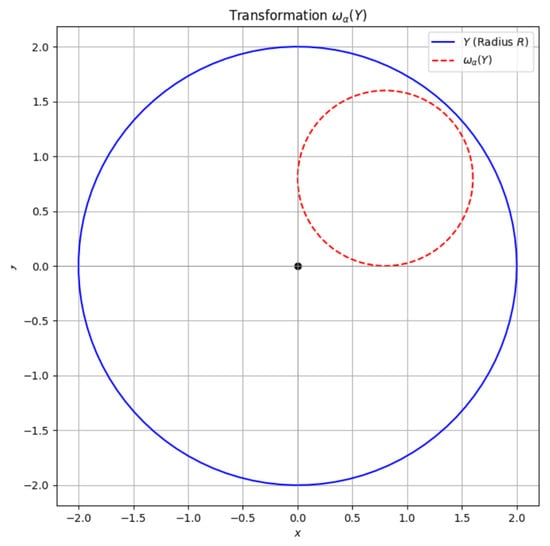
Figure 1. Plot 1.

Explanation: Visualization of the ball Y (blue) with radius R and its image under the mapping ${\omega }_{\alpha }\left(Y\right)$ (red, dashed). The mapping ${\omega }_{\alpha }$ transforms points within Y while considering the constants r and $\gamma$. The source code in Python for this plots and mappings is provided in the Appendix A.

Plot 2: Applying $T_n$ to ${\omega }_{\alpha }\left(Y\right)$ (Figure 2).

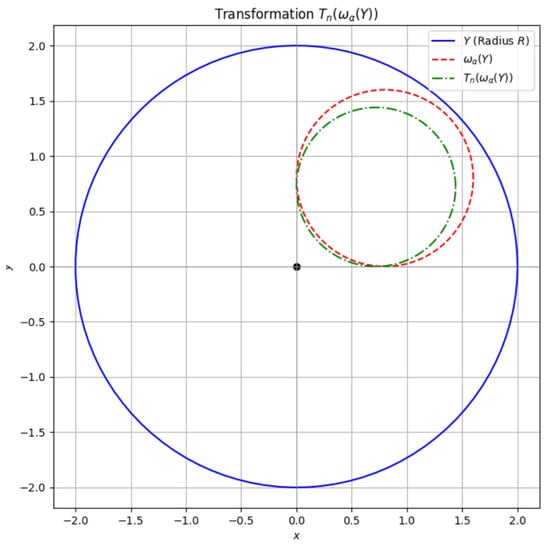
Figure 2. Plot 2.

Explanation: Visualization of the ball Y (blue) with radius R, the image ${\omega }_{\alpha }\left(Y\right)$ (red, dashed), and the subsequent image $T_n\left({\omega }_{\alpha }\left(Y\right)\right)$ (green, dot–dashed). The transformation $T_n$ maps the image of ${\omega }_{\alpha }$ back into the ball Y, illustrating the condition $T_n\left({\omega }_{\alpha }\left(Y\right)\right)\subset Y$. The source code in Python for this plots and mappings is provided in the Appendix A.

6.3. Example of Computing the Monge–Kantorovich Norm for a Dirac Measure in a Hilbert Space

Here, we give an example of computing the Monge–Kantorovich norm for a certain measure. Let $(X,⟨·,·⟩)$ be a Hilbert space, $T=[0,1],t\in T,\mu :\mathcal{B}\to X,\mu ={\delta }_t·x,{\delta }_t$ being the Dirac measure concentrated in t and $x\in X$ such that $\parallel x\parallel =1$. If $f\in B{L}_1\left(X\right)$, we have $\left|\int fd\mu \right|=\left|⟨f\left(t\right),x⟩\right|\le {\parallel f\parallel }_{BL}·\parallel x\parallel \le 1$; hence, ${\parallel \mu \parallel }_{MK}\le 1$. Now, taking $f\left(t\right)=x,\forall t\in T$, we have ${\parallel f\parallel }_{BL}={\parallel f\parallel }_{\infty }=\parallel x\parallel =1$ and $\left|\int fd\mu \right|=⟨x,x⟩={\parallel x\parallel }^2=1$; hence, ${\parallel \mu \parallel }_{MK}\ge 1$. We conclude that ${\parallel \mu \parallel }_{MK}=1$.

6.4. Example of Norm Computation for Linear Operators in ${\mathbb{R}}^2$

Let us define ${\omega }_{\alpha }:{\mathbb{R}}^2\to {\mathbb{R}}^2,{\omega }_{\alpha }(x,y)=\frac{1}{2^{\alpha }}(y,x),\alpha \in [1,2],T_n:{\mathbb{R}}^2\to {\mathbb{R}}^2,T_n(x,y)=\frac{1}{n}(x-y,x+y),n\in {\mathbb{N}}^{*}$. Obviously, $r_{\alpha }=\frac{1}{2^{\alpha }},r=\underset{\alpha \in [1,2]}{sup}{r}_{\alpha }=\frac{1}{2}$. Let us compute $\parallel T_n\parallel$. In fact, we have $T_n=\frac{1}{n}·T,T$ being the operator given by the matrix $A=\left(\begin{array}{cc}1& -1\\ 1& 1\end{array}\right)$. It is known that if $T:{\mathbb{R}}^k\to {\mathbb{R}}^k$ is a linear operator given by a matrix A, we have $\parallel T\parallel ={\left(\underset{{\lambda }_j}{sup}\left|{\lambda }_j\right|\right)}^{\frac{1}{2}},{\lambda }_j$ being the eigenvalues of the matrix $A^t·A$ where $A^t$ is the transpose of A. In our case, it is easy to obtain $\parallel T\parallel =\sqrt{2}$; so, we have $\parallel T_n\parallel =\frac{\sqrt{2}}{n}$. Thus, $\beta =\underset{n\ge 1}{sup}\frac{\sqrt{2}}{n}=\sqrt{2}$ and $\beta r=\frac{1}{\sqrt{2}}<1$. Let us consider the operators ${\left(R_{\alpha }\right)}_{\alpha \in [1,2]},R_{\alpha }:{\mathbb{R}}^2\to {\mathbb{R}}^2,R_{\alpha }(x,y)=\frac{1}{3{\alpha }^2}(x+2y,y)$. Using the formula as above, we obtain $\parallel R_{\alpha }\parallel =\frac{1}{3{\alpha }^2}(1+\sqrt{2})$. We have ${\int }_1^2\parallel R_{\alpha }\parallel \parallel (1+\beta r_{\alpha })\parallel d\alpha \le \left(\sqrt{2}+1\right)\left(1+\frac{1}{\sqrt{2}}\right)·\frac{1}{3}{\int }_1^2\frac{1}{{\alpha }^2}d\alpha =\frac{1}{6}·\frac{{(\sqrt{2}+1)}^2}{\sqrt{2}}<1$. Hence, the conditions for the Theorems 7 and 8 are fulfilled.

6.5. Example of Variational Norm Computation for a Measure in ${\mathbb{R}}^2$

Let us take ${\mu }^{\circ }=\frac{1}{8}\nu$, where $\nu :\mathcal{B}\to {\mathbb{R}}^2,\nu \left(A\right)=(\lambda \left(A\right),{\delta }_0\left(A\right))$, A is a Borel subset of $T=[0,1]$, $\lambda$ is the Lebesgue measure, and ${\delta }_0$ is the Dirac measure concentrated in 0. We will compute the variational norm of ${\mu }^{\circ }$, that is, $\left|\mu \right|\left(T\right)$. We have $\left|\nu \right|\left(\right[0,1\left]\right)=\left|\nu \right|\left(\right(0,1\left]\right)+\left|\nu \right|\left(\right\{0\left\}\right)$. But, $\nu \left(\left\{0\right\}\right)=(\lambda \left(\left\{0\right\}\right),{\delta }_0\left(\left\{0\right\}\right)=(0,1)$; hence, $\left|\nu \right|\left(\right\{0\left\}\right)=\parallel (0,1)\parallel =1$. For computing $\left|\nu \right|\left(\right(0,1\left]\right)$, we see that for any Borel $A\subset (0,1],\nu \left(A\right)=(\lambda \left(A\right),{\delta }_0\left(A\right))=(\lambda \left(A\right),0)$; so, $\parallel \nu \left(A\right)\parallel =\lambda \left(A\right)$. Taking a partition ${\left(A_j\right)}_j$ of A with Borel sets, we see that ${\displaystyle \sum _j}\parallel \nu \left(A_j\right)\parallel ={\displaystyle \sum _j}\lambda \left(A_j\right)=\lambda \left(A\right)$.

Hence, $\left|\nu \right|\left(A\right)={\displaystyle \underset{{\left(A_{\mathrm{j}}\right)}_{\mathrm{j}}\mathrm{finite}\mathrm{partition}\mathrm{of}A\mathrm{with}\mathrm{Borel}\mathrm{subsets}}{sup}}\left\{{\displaystyle \sum _j}\parallel \nu \left(A_j\right)\parallel \right\}=\lambda \left(A\right)$.

We deduce that $\left|\nu \right|\left(\right(0,1\left]\right)=\lambda \left(\right(0,1\left]\right)=1$ and $\left|\nu \right|\left(\right[0,1\left]\right)=1+1=2$; hence, $\left|{\mu }^{\circ }\right|\left([0,1]\right)=\frac{1}{4}=∥{\mu }^{\circ }∥$. Taking ${\omega }_{\alpha }$ and $R_{\alpha }$ from example 6.4 and $c=1$ we will have $∥{\mu }^{\circ }∥+c{\int }_1^2\parallel R_{\alpha }\parallel (1+r_{\alpha })d\alpha =\frac{1}{4}+{\int }_1^2\frac{1}{3{\alpha }^2}(1+\sqrt{2})\left(\frac{1}{2^{\alpha }}+1\right)d\alpha \le \frac{1}{4}+\frac{1}{3}·\frac{3}{2}(\sqrt{2}+1){\int }_1^2\frac{1}{{\alpha }^2}d\alpha <1$. Using Remark 2, we can take $\overline{B}=B_1\left({\mathbb{R}}^n\right)$ and the hypothesis from Theorem 6 is fulfilled.

6.6. Analysis of Operators $T_n$ in $L^2$ Spaces

We denote $L^2\stackrel{not}{=}{L}^2\left([0,1]\right)$ (taking into account the Lebesgue measure on $[0,1]$). Let us define the operators: $T_n\left(f\right)\left(x\right)=\left\{\begin{array}{c}f\left(x\right),\mathrm{if}x\in \left(\frac{1}{n},1\right]f\left(x\right)·n^a,\mathrm{if}x\in \left[0,\frac{1}{n}\right],(a>0)\hfill \end{array}\right.$ and $T\left(f\right)=f$, for any $f\in L^2$.

(1°)

We consider the case $a>\frac{1}{2}$ and we will prove that there exists $f\in L^2$ such that $T_n\left(f\right)\notin L^2$. Indeed, if $f\left(x\right)=1,\forall x\in [0,1]$, we have

$$\underset{[0,1]}{\int }{\left|T_n\left(f\right)\left(x\right)\right|}^{2}d\lambda \left(x\right)\ge \underset{\left[0,\frac{1}{n}\right]}{\int }{n}^{2a}d\lambda \left(x\right)=n^{2a-1}\to \infty \mathrm{if}n\to \infty .$$

(2°)

Let us now consider $a=\frac{1}{2}$.

(i)

We prove that $T_n\left(f\right)\in L^2$ for any $f\in L^2$:

$$\underset{[0,1]}{\int }{\left|T_n\left(f\right)\left(x\right)\right|}^{2}d\lambda \left(x\right)=\underset{\left[0,\frac{1}{n}\right]}{\int }n{f}^2\left(x\right)d\lambda \left(x\right)+\underset{\left[\frac{1}{n},1\right]}{\int }{f}^2\left(x\right)d\lambda \left(x\right).$$

With the space $C\left(\right[0,1\left]\right)$ being dense in $L^1\left((0,1]\right)$, we will find a sequence ${\left(F_k\right)}_k\subset C\left([0,1]\right)$ such that $F_k\underset{k}{\overset{L^1\left([0,1]\right)}{\to }}{f}^2$ and then a subsequence ${\left(F_{k_j}\right)}_j\subset {\left(F_k\right)}_k$ and a Borel set $A\subset [0,1]$ with the following properties:

(a)

$\lambda \left(A\right)=0$;

(b)

$\underset{j\to \infty }{lim}{F}_{k_j}\left(x\right)=f^2\left(x\right),\forall x\in [0,1]\setminus A$.

Taking $\epsilon >0$ (arbitrarily, fixed), we will find $k_j\in \mathbb{N}$ such that $|F_{k_j}\left(x\right)-f^2\left(x\right)|<\epsilon ,\forall x\in [0,1]\setminus A$. Let us denote $M=\underset{x\in \left[0,\frac{1}{n}\right]}{max}\left|F_{k_j}\left(x\right)\right|$. We have

$$\underset{\left[0,\frac{1}{n}\right]}{\int }n{f}^2\left(x\right)d\lambda \left(x\right)\le \underset{\left[0,\frac{1}{n}\right]}{\int }n\left|f^2\left(x\right)-F_{k_j}\left(x\right)\right|d\lambda \left(x\right)+n\underset{\left[0,\frac{1}{n}\right]}{\int }\left|F_{k_j}\left(x\right)\right|d\lambda \left(x\right)\le$$

$$\le M·n·\frac{1}{n}+\underset{=0}{\underbrace{\underset{\left[0,\frac{1}{n}\right]\cap A}{\int }n\left|f^2\left(x\right)-F_{k_j}\left(x\right)\right|d\lambda \left(x\right)}}+\underset{\left[0,\frac{1}{n}\right]\setminus A}{\int }n\left|f^2\left(x\right)-F_{k_j}\left(x\right)\right|d\lambda \left(x\right)\le$$

$\le M+n\epsilon \frac{1}{n}=M+\epsilon$. Thus, we have $\underset{[0,1]}{\int }|T_n{\left(f\right)\left(x\right)|}^{2}d\lambda \left(x\right)\le M+\epsilon +{\parallel f\parallel }_2<\infty$; hence, $T_n\left(f\right)\in L^2$.

(ii)

Let us again consider $f\left(x\right)=1,\forall x\in [0,1]$.

$$\parallel (T_n-T)\left(f\right){\parallel }_2^2=\underset{\left[0,\frac{1}{n}\right]}{\int }{|f\left(x\right)\sqrt{n}-f\left(x\right)|}^{2}d\lambda \left(x\right)=\frac{1}{n}{(\sqrt{n}-1)}^2;$$

Then, $\underset{{\parallel f\parallel }_2\le 1}{sup}\parallel (T_n-T)\left(f\right)\parallel \ge {\left(\frac{{(\sqrt{n}-1)}^2}{n}\right)}^{\frac{1}{2}}$ and $\underset{n\to \infty }{lim}\frac{{(\sqrt{n}-1)}^2}{n}=1$. Consequently, $T_n\stackrel{{\parallel ·\parallel }_{\circ }}{\cancel{\to }}T$.

(iii)

We prove that $T_n\to T$ is the topology of weak convergence of the operators. Let $g\in {\left(L^2\right)}^{*}=L^2,f\in L^2$. We have

$$|g\left(T_n\left(f\right)\right)-g\left(T\left(f\right)\right)|=|g(T_n\left(f\right)-f)|=\left|{\int }_{\left[0,\frac{1}{n}\right]}g\left(x\right)f\left(x\right)(\sqrt{n}-1)d\lambda \left(x\right)\right|;$$

similar to point (i), we find a sequence ${\left(h_j\right)}_j)\subset C\left([0,1]\right)$ and a Borel set $B\subset [0,1]$ such that $\lambda \left(B\right)=0$ and $\underset{j\to \infty }{lim}{h}_j\left(x\right)=f\left(x\right)g\left(x\right),\forall x\in [0,1]\setminus B$. Let $\epsilon >0$ (arbitrarily, fixed). We will find $j\in \mathbb{N}$ such that $|h_j\left(x\right)-f\left(x\right)g\left(x\right)|<\epsilon ,\forall x\in [0,1]\setminus B$. We have

$$\underset{\left[0,\frac{1}{n}\right]}{\int }\left|f\left(x\right)g\left(x\right)\right|(\sqrt{n}-1)d\lambda \left(x\right)\le \underset{=0}{\underbrace{\underset{\left[0,\frac{1}{n}\right]\cap B}{\int }|f\left(x\right)g\left(x\right)-h_j\left(x\right)|(\sqrt{n}-1)d\lambda \left(x\right)}}+$$

$$+\underset{\left[0,\frac{1}{n}\right]\setminus B}{\int }|f\left(x\right)g\left(x\right)-h_j\left(x\right)|(\sqrt{n}-1)d\lambda \left(x\right)+(\sqrt{n}-1)\underset{\left[0,\frac{1}{n}\right]}{\int }\left|h_j\left(x\right)\right|d\lambda \left(x\right)\le$$

$$\le \left(\frac{1}{n}·\epsilon +\frac{1}{n}\underset{x\in [0,1]}{max}{h}_j\left(x\right)\right)(\sqrt{n}-1)\to 0,\mathrm{as}n\to \infty .$$

Hence, for $f\in L^2$ and for any $g\in {\left(L^2\right)}^{*}=L^2$, $g\left(T_n\left(f\right)\right)\to g\left(T\left(f\right)\right)$, that is, $T_n\to T$ in the topology of the weak convergence of the operators.

(3°)

If $a\in \left(0,\frac{1}{2}\right)$, in the same way as in $2^{\circ },\left(iii\right)$ one can prove that $T_n\to T$ in the topology of the weak convergence of the operators.

7. Conclusions

In this paper, we have extended the classical theory of iterated function systems in three significant ways:

(a)

Unlike the traditional approach, which employs a finite set of contractions, we have explored the construction of iterated function systems using an uncountable set of contractions, broadening the scope of applicability.

(b)

Our investigation introduces a novel perspective on fractal measures by considering them as vector measures rather than the classical positive normalized measures. This expanded understanding opens up new avenues for analysis and application.

(c)

Furthermore, we have delved into the study of sequences of (uncountable) iterated function systems, examining various convergence properties. This adds depth to our understanding of the behavior and limitations of such systems.

Moving forward, our focus will be on addressing two key questions:

(1°)

We will delve into the problem of convergence concerning the sequences of attractors and fractal vector measures within a broader framework. This inquiry aims to provide insights into the stability and long-term behavior of these systems under diverse conditions.

(2°)

Additionally, we will explore the application of our findings to the theory of differential equations. By bridging the gap between fractal geometry and differential equations, we aim to uncover new perspectives and potential applications in areas such as dynamical systems and mathematical modeling.

By addressing these questions, we seek to not only advance the theoretical understanding of iterated function systems but also to uncover practical implications that could impact various fields of science and mathematics.

References

- Mierlus-Mazilu, I.; Nită, L. Sequences of Uncountable Iterated Function Systems: The Convergence of the Sequences of Fractals and Fractal Measures Associated. In Mathematical Methods for Engineering Applications (Springer Proceedings in Mathematics & Statistics); Springer: Cham, Switzerland, 2024; Volume 439, pp. 43–52. [Google Scholar]
- Chițescu, I. Spații de Funcții; Ed. Științifică și Enciclopedică: Bucharest, Romania, 1983. [Google Scholar]
- Chițescu, I.; Ioana, L.; Miculescu, R.; Niță, L. Sesquilinear uniform vector integral. Proc. Indian Acad. Sci. (Math. Sci.) 2015, 125, 229–236. [Google Scholar] [CrossRef]
- Chițescu, I.; Ioana, L.; Miculescu, R.; Niță, L. Monge–Kantorovich norms on spaces of vector measures. Results Math. 2016, 70, 349–371. [Google Scholar] [CrossRef]
- Cobzas, S.; Miculescu, R.; Nicolae, A. Lipschitz Functions; Lecture Notes in Mathematics; Springer International Publishing: New York, NY, USA, 2019; pp. 365–556. [Google Scholar]
- D’Aniello, E.; Steele, T.H. Attractors for classes of iterated function systems. Eur. J. Math. 2019, 5, 116–137. [Google Scholar] [CrossRef]
- Mendivil, F.; Vrscay, E.R. Self-affine vector measures and Vector Calculus on Fractals. Fractals Multimed. 2002, 132, 137–155. [Google Scholar]
- Mierluș-Mazilu, I.; Niță, L. About Some Monge–Kantovorich Type Norm and Their Applications to the Theory of Fractals. Mathematics 2022, 10, 4825. [Google Scholar] [CrossRef]
- Mihail, A. Recurrent iterated function systems. Rev. Roumaine Math. Pures Appl. 2008, 53, 43–53. [Google Scholar]
- Sirețchi, G. Spatii Concrete in Analiza Funcționala; Centrul de Multiplicare al Universitatii Bucuresti: Bucharest, Romania, 1982. (In Romanian) [Google Scholar]
- Igbida, N.; Mazón, J.M.; Rossi, J.D.; Toledo, J. A Monge–Kantorovich mass transport problem for a discrete distance. J. Funct. Anal. 2011, 260, 494–3534. [Google Scholar] [CrossRef]
- La Torre, D.; Maki, E.; Mendivil, F.; Vrscay, E.R. Iterated function systems with place-dependent probabilities and the inverse problem of measure approximation using moments. Fractals 2018, 26, 1850076. [Google Scholar] [CrossRef]
- Mendivil, F. Computing the Monge–Kantorovich distance. Comput. Appl. Math. 2017, 36, 1389–1402. [Google Scholar] [CrossRef]
- Rachev, S.T.; Klebanov, L.B.; Stoyanov, S.V.; Fabozzi, F.J. Monge–Kantorovich Mass Transference Problem, Minimal Distances and Minimal Norms. In The Methods of Distances in the Theory of Probability and Statistics; Springer: New York, NY, USA, 2013. [Google Scholar]
- Strobin, F. On the existence of the Hutchinson measure for generalized iterated function systems. Qual. Theory Dyn. Syst. 2020, 19, 1–21. [Google Scholar] [CrossRef]
- Secelean, N.A. Măsură și Fractali; Ed. Universității Lucian Blaga: Sibiu, Romania, 2002. [Google Scholar]
- Niță, L. Fractal Vector Measures in the case of an Uncountable Iterated Function System. RJM-CS 2015, 5, 151–163. [Google Scholar]
Disclaimer/Publisher’s Note: The statements, opinions and data contained in all publications are solely those of the individual author(s) and contributor(s) and not of MDPI and/or the editor(s). MDPI and/or the editor(s) disclaim responsibility for any injury to people or property resulting from any ideas, methods, instructions or products referred to in the content. |
© 2024 by the authors. Licensee MDPI, Basel, Switzerland. This article is an open access article distributed under the terms and conditions of the Creative Commons Attribution (CC BY) license (https://creativecommons.org/licenses/by/4.0/).