Testing a Class of Piece-Wise CHARN Models with Application to Change-Point Study

Abstract

We study a likelihood ratio test for testing the conditional mean of a class of piece-wise stationary CHARN models. We establish the locally asymptotically normal (LAN) structure of the family of likelihoods under study. We prove that the test is asymptotically optimal, and we give an explicit form of its asymptotic local power. We describe an algorithm for detecting change points and estimating their locations. The estimates are obtained as time indices, maximizing the estimate of the local power. The simulation study we conduct shows the good performance of our method on the examples considered. This method is also applied to a set of financial data.

1. Introduction

Let $d,p,k,n\in \mathbb{N}$ and $k<<n$. Assume the observations $X_1,\dots ,X_n$ issued from the following piece-wise stationary CHARN model (see, e.g., [1])

$$X_t=T({\mathit{\rho }}_0+\mathit{\gamma }\odot \omega \left(t\right);{\mathbf{X}}_{t-1})+V\left({\mathbf{X}}_{t-1}\right){\epsilon }_t,t\in \mathbb{Z},$$

(1)

with

$$\begin{array}{cc}\hfill X_t& =Y_{t,j}=T({\mathit{\rho }}_{\mathbf{0}}+{\mathit{\gamma }}_j{\omega }_j\left(t\right);{\mathbf{X}}_{t-1,j})+V\left({\mathbf{X}}_{t-1,j}\right){\epsilon }_t,{\tau }_{j-1}\le t<{\tau }_j,\hfill \\ & j=1,\dots ,k+1,\hfill \end{array}$$

(2)

where for $j=1,\dots ,k,$ ${\left(Y_{t,j}\right)}_{t\in \mathbb{Z}}$ is a stationary and ergodic process; ${\mathit{\rho }}_0\in {\mathbb{R}}^p$, $T({\mathit{\rho }}_0,.)$ and $V(.)$ are real-valued functions with ${inf}_{x\in {\mathbb{R}}^d}V\left(x\right)>0;$ the ${\tau }_j$, $j=0,\dots ,k+1$, are potential instants of changes with ${\tau }_0=1$ and ${\tau }_{k+1}=n+1$; for $j=1,\dots ,k,$ ${\mathbf{X}}_{t,j}={(Y_{t,j},\dots ,Y_{t-d+1,j})}^{\top }$, ${\mathbf{X}}_{{\tau }_{j-1}+\ell }={\mathbf{X}}_{{\tau }_{j-1}+\ell ,j},\ell =0,\dots ,d-1$ and for $t\in [{\tau }_{j-1}+d-1,{\tau }_j),{\mathbf{X}}_t={(X_t,\dots ,X_{t-d+1})}^{\top }$; for $j,\ell =1,\dots ,k,j\ne \ell ,$ the processes ${\left(Y_{t,j}\right)}_{t\in \mathbb{Z}}$ and ${\left(Y_{t,\ell }\right)}_{t\in \mathbb{Z}}$ are mutually independent; ${\left({\epsilon }_t\right)}_{t\in \mathbb{Z}}$ is standard white noise with density f. $\mathit{\gamma }={\left({\mathit{\gamma }}_1^{\top },\dots ,{\mathit{\gamma }}_{k+1}^{\top }\right)}^{\top }$, ${\mathit{\gamma }}_j\in {\mathbb{R}}^p$, $j=1,\dots ,k+1$; $\omega \left(t\right)=({\mathbf{1}}_{[{\tau }_0,{\tau }_1)}\left(t\right),{\mathbf{1}}_{[{\tau }_1,{\tau }_2)}\left(t\right),\dots ,{\mathbf{1}}_{[{\tau }_{k-1},{\tau }_k)}\left(t\right)$, ${\mathbf{1}}_{[{\tau }_k,{\tau }_{k+1})}{\left(t\right))}^{\top }=({\omega }_1\left(t\right),\dots ,{\omega }_{k+1}\left(t\right))\in {\{0,1\}}^{k+1}$; for $\mathit{\gamma }={\left({\mathit{\gamma }}_1^{\top },\dots ,{\mathit{\gamma }}_{k+1}^{\top }\right)}^{\top }$ and $\omega \left(t\right)={\left({\omega }_1\left(t\right),\dots ,{\omega }_{k+1}\left(t\right)\right)}^{\top }$, $\mathit{\gamma }\odot \omega \left(t\right)$ stands for $\mathit{\gamma }\odot \omega \left(t\right)={\mathit{\gamma }}_1{\omega }_1\left(t\right)+\dots +{\mathit{\gamma }}_{k+1}{\omega }_{k+1}\left(t\right)\in {\mathbb{R}}^p,$ and ${\mathit{\gamma }}_i{\omega }_i=({\gamma }_{i,1}{\omega }_i,\dots ,{\gamma }_{i,p}{\omega }_i)\in {\mathbb{R}}^p.$ The class of models (2) is very large. It contains models such as AR(p), ARCH(p), EXPAR(p), and GEXPAR(p) whose statistical and probability properties are widely studied in the literature (see, e.g., [2] for a study of the ergodicity of GEXPAR models).

As noted in [3], the assumption that ${\left({\mathbf{X}}_{t,j}\right)}_{t\in \mathbb{Z}}$ and ${\left({\mathbf{X}}_{t,\ell }\right)}_{t\in \mathbb{Z}}$ are independent can be extended to some weak dependence assumption. In this paper, for ${\mathit{\gamma }}_0\in {\mathbb{R}}^{p(k+1)}$ and $\mathit{\beta }\in {\mathbb{R}}^{p(k+1)}$ depending on the ${\tau }_j$s, we construct a likelihood ratio test for testing

$$H_0:\mathit{\gamma }={\mathit{\gamma }}_0\mathrm{against}{H}_{\mathit{\beta }}^{\left(n\right)}:\mathit{\gamma }={\mathit{\gamma }}_n={\mathit{\gamma }}_0+{\displaystyle \frac{\mathit{\beta }}{\sqrt{n}}}.$$

(3)

A particular case of this work is studied in [4]. The literature on change points is extensive and varied. Some basic notions and theory are presented in [5], where one can find number of references on the first works on the subject. Most of the recent papers on change points are in time series or regression contexts. Various methods and techniques are used for the study. Ref. [6] proposes a test for parameter changes. The observations are assumed to follow an exponential distribution. The author presents a derivation using the method of [7]. Ref. [8] studies the problem of changes in the parameters of AR models and the variance in the white noise using the likelihood ratio statistic. Ref. [9] proposes test statistics for detecting a break in the trend function of a dynamic univariate time series. The tests are based on the mean and exponential statistics of [10] and the supremum statistic of [11]. Another method for detecting change points is introduced in [12]. The authors present a multiple-change-point analysis for which the Markov Chain Monte Carlo (MCMC) sampler plays a fundamental role. They propose an attractive methodology for the change-point problem in a Bayesian context. The reversible jump algorithm is presented. Ref. [13] also studies the problem of detecting change points in the mean of a signal corrupted by additive noise. The number of change points is estimated by a method based on a penalized least-square criterion. Ref. [14] uses the minimum description length for detecting change points for a non-stationary time series with an application to GARCH models, stochastic volatility models and generalized state-space models as the parametric model for the segments. Ref. [15] uses maximum likelihood to estimate the instant of the change. The authors study the asymptotic distribution of their test by contiguity. Ref. [16] investigates the regression function or its $\nu$th derivative in generalized linear models which may have a change (discontinuity) point at an unknown location. Ref. [17] studies change points in the mean of a sequence of independent normally distributed random vectors. The asymptotic distribution of the test statistic is studied by using results from [18]. Also, Ref. [19] studies this problem for independent normal means as a multiple testing problem. The authors consider two stepwise methods, the binary segmentation method of [20] and the maximum residual down method of [21]. They prove the consistency of these methods. Ref. [22] studies the existence of changes in the regression parameters in a linear model where the regressors and errors are weakly dependent. They study the asymptotic distribution under the null hypothesis and under contiguous alternatives. In [23], the authors develop a method for detecting and estimating change points in the tail of multiple time series data. They discuss the effect of the mean and variance’s change on the tails. They focus on the detection of change points in the upper tail of the distribution of the variable of interest, based on multiple cross-sectional time series. Ref. [24] proposes a procedure based on the Bayesian information criterion ($BIC$) in combination with the binary segmentation algorithm to look for changes in the mean, autoregressive coefficients, and variance in the perturbation in piecewise autoregressive processes. The authors explain briefly the Auto-PARM and Auto-SLEX methods. They present different algorithms useful to the search of multiple change points. Ref. [25] proposes a likelihood ratio scan method for estimating multiple change points in piecewise stationary processes. Ref. [26] aims to estimate the instant of change in a regression model. The authors use a sequential Bayesian change-point algorithm that provides uncertainty bounds on both the number and location of the change. A class of change-point test statistics is proposed in [27] that utilizes a weighting and trimming scheme for the cumulative sum (CUSUM) process inspired by Renyi. Using an asymptotic analysis and simulations, the authors demonstrate that this class of statistics possesses superior power compared to traditional change-point statistics based on the CUSUM process, when the change point is near the beginning or end of the sample. The authors develop a generalization of these "Renyi” statistics for testing for changes in the parameters of linear and non-linear regression models, and in the generalized method of moment estimation.

In this paper, we are interest in weak change detection. A weak change is one with a too-small magnitude. Such a change may be a harbinger signaling a forthcoming critical behavior of the phenomenon studied. It can manifest in various domains including economics and finance, public health, bio-science, engineering, climatology, hydrology, linguistics, genomics, signal processing and many others.

Classical change detection methods can fail in detecting weak changes. Therefore, it may be of importance to develop new methods for their detection. In the context of time series, very few studies have tested no change against local alternatives of weak changes. Refs. [4,28] study this problem for the case of testing the mean of the model (1). As changes can happen elsewhere than the mean, it can be interesting to study more general models. Our main purpose in this paper is to extend these works to the conditional mean of (1). With this purpose, we proceed with the same techniques. We first construct a test based on the likelihood ratio, and we study its null distribution. Next, we establish the LAN property for the likelihood families under study. From this, we prove the contiguity of $H_0$ and $H_{\mathit{\beta }}^{\left(n\right)}$ and use it together with Le Cam’s third lemma to find the asymptotic distribution of the test under $H_{\mathit{\beta }}^{\left(n\right)}$. Then, we prove the optimality of our test in the case in which the parameters are known. In the case that the parameters are assumed to be unknown, we prove the convergence of the estimated version of the central sequence based on the parameter estimators to its true version. Finally, we prove that the test remains optimal in the case of unknown parameters. Based on the explicit expression of the power, we construct an algorithm for detecting change points and estimating their locations. The simulation study shows the good performance of our method for detecting weak changes and estimating their locations in the examples considered.

In Section 2, we specify the notation and list some of the main assumptions. In Section 3, we state the theoretical results in the case that ${\mathit{\rho }}_0$ is known and in the case that it is unknown. The results of this section are used in Section 4 to construct an algorithm for testing change points and estimating their locations. In Section 5, a simulation experiment is conducted for the application of our algorithm. Section 6 concludes our work, and the last section contains the proofs of the results stated in Section 3.

2. Notation and Assumptions

In this section, we specify the notation and list some of the main assumptions needed.

2.1. The Notation

In the sequence, ${\mathcal{M}}_{m,n}\left(\mathbb{R}\right)$ is the space of real $m\times n$ matrices and ${\mathcal{M}}_n\left(\mathbb{R}\right)={\mathcal{M}}_{n,n}\left(\mathbb{R}\right)$. $M^{\top }$ is the transpose of $M\in {\mathcal{M}}_{m,n}\left(\mathbb{R}\right)$, and $\left|\right|\left|M\right||{|}_{m\times n}$ is its Euclidean matrix norm. ${\parallel .\parallel }_p$ is the Euclidean norm of ${\mathbb{R}}^p$.

Let $U\in {\mathbb{R}}^{p(k+1)}$; we write $U={\left(U_1^{\top },\dots ,U_{k+1}^{\top }\right)}^{\top }$ and for any $i\in \{1,\dots ,k+1\}$,

$$\begin{array}{c}\hfill U_i={\left(U_{i1},\dots ,U_{ip}\right)}^{\top }.\end{array}$$

For $M\in {\mathcal{M}}_{p(k+1)}\left(\mathbb{R}\right)$, we write

$$\begin{array}{c}\hfill M=\left(\begin{array}{ccc}{M}_{1,1}& \dots & M_{1,k+1}\\ ⋮& \ddots & ⋮\\ M_{k+1,1}& \dots & M_{k+1,k+1}\end{array}\right),\end{array}$$

where for $i,j\in \{1,\dots ,k+1\}$, $M_{i,j}\in {\mathcal{M}}_p\left(\mathbb{R}\right)$.

Let $\Im :{\mathbb{R}}^d\to \mathbb{R}$ be a differentiable function on ${\mathbb{R}}^d$. For any $\mathit{\gamma }\in {\mathbb{R}}^{p(k+1)}$, we denote by $D_{\mathit{\gamma }}[\Im ]$ the following matrix:

$$D_{\mathit{\gamma }}[\Im \left(x\right)]={\left({\partial }_{{\mathit{\gamma }}_1}[\Im \left(x\right)],\dots ,{\partial }_{{\mathit{\gamma }}_{k+1}}[\Im \left(x\right)]\right)}^{\top }\in {\mathbb{R}}^{p(k+1)},$$

where ${\partial }_{{\mathit{\gamma }}_i}[\Im \left(x\right)]$ is the gradient of ℑ with respect to ${\gamma }_i$ at $x\in {\mathbb{R}}^d$:

$${\partial }_{{\mathit{\gamma }}_i}[\Im \left(x\right)]={\left({\displaystyle \frac{\partial \Im }{\partial {\mathit{\gamma }}_{i,1}}}\left(x\right),{\displaystyle \frac{\partial \Im }{\partial {\gamma }_{i,2}}}\left(x\right),\dots ,{\displaystyle \frac{\partial \Im }{\partial {\gamma }_{i,p}}}\left(x\right)\right)}^{\top }\in {\mathbb{R}}^p,$$

where for $i=1,\dots ,k+1$ and $j=1,\dots ,p$, ${\displaystyle \frac{\partial \Im }{\partial {\gamma }_{i,j}}}$ is the partial derivative of ℑ with respect to ${\gamma }_{i,j}$.

We also denote by $H_{\mathit{\gamma }}\left[\Im \left(x\right)\right]$ the matrix

$$H_{\mathit{\gamma }}\left[\Im \left(x\right)\right]=\left(\begin{array}{ccc}{\partial }_{{\mathit{\gamma }}_1{\mathit{\gamma }}_1}^2\Im \left(x\right)& \dots & {\partial }_{{\mathit{\gamma }}_1{\mathit{\gamma }}_{k+1}}^2\Im \left(x\right)\\ ⋮& \ddots & ⋮\\ {\partial }_{{\mathit{\gamma }}_{k+1}{\mathit{\gamma }}_1}^2\Im \left(x\right)& \dots & {\partial }_{{\mathit{\gamma }}_{k+1}{\mathit{\gamma }}_{k+1}}^2\Im \left(x\right)\end{array}\right)\in {\mathcal{M}}_{p(k+1)}\left(\mathbb{R}\right),x\in {\mathbb{R}}^d$$

where, for every $i\in \{1,\dots ,k+1\},$

$${\partial }_{{\mathit{\gamma }}_i{\mathit{\gamma }}_j}^2\Im \left(x\right)=\left(\begin{array}{ccc}{\displaystyle \frac{{\partial }^2\Im }{\partial {\gamma }_{i,1}\partial {\gamma }_{j,1}}}\left(x\right)& \dots & {\displaystyle \frac{{\partial }^2\Im }{\partial {\gamma }_{i,p}\partial {\gamma }_{j,1}}}\left(x\right)\\ ⋮& \ddots & ⋮\\ {\displaystyle \frac{{\partial }^2\Im }{\partial {\gamma }_{i,1}\partial {\gamma }_{j,p}}}\left(x\right)& \dots & {\displaystyle \frac{{\partial }^2\Im }{\partial {\gamma }_{i,p}\partial {\gamma }_{j,p}}}\left(x\right)\end{array}\right)\in {\mathcal{M}}_p\left(\mathbb{R}\right),x\in {\mathbb{R}}^d.$$

We denote any differentiable function g with derivative $g^{\prime }$ by

$$\begin{array}{c}\hfill {\displaystyle {\varphi }_g=-{\displaystyle \frac{g^{\prime }}{g}}\mathrm{and} I\left(g\right)={\int }_{\mathbb{R}}{\varphi }_g^2\left(x\right)g\left(x\right)dx.}\end{array}$$

For any $t\in \{1,\dots ,n\}$, let ${\mathcal{F}}_t=\sigma ({\mathbf{X}}_1,\dots ,{\mathbf{X}}_t)$ be the $\sigma$-algebra generated by ${\mathbf{X}}_1,\dots ,{\mathbf{X}}_t$ such that ${\epsilon }_t$ is independent of ${\mathcal{F}}_{t-1}$.

2.2. The Main Assumptions

In this section, we outline the key assumptions needed for our methodology. These are crucial for establishing our theoretical results. Following their enumeration, we include a remark that articulates their significance. So, we assume that

(A₁) 

${\displaystyle {\int }_{\mathbb{R}}xf\left(x\right)dx=0}$ and ${\displaystyle {\int }_{\mathbb{R}}{x}^{2}f\left(x\right)dx=1}$.

(A₂) 

f is differentiable with derivative $f^{\prime }$.

(A₃) 

${\displaystyle \underset{x\to +\infty }{lim}f\left(x\right)=\underset{x\to -\infty }{lim}f\left(x\right)=0=\underset{x\to +\infty }{lim}{f}^{\prime }\left(x\right)=\underset{x\to -\infty }{lim}{f}^{\prime }\left(x\right).}$

(A₄) 

${\varphi }_f$ is differentiable with derivative ${\varphi }_f^{\prime }$ and is $c_{\varphi }$-Lipschitz where $0<c_{\varphi }<+\infty .$

(A₅) 

$max\left\{{\displaystyle {\int }_{\mathbb{R}}|{\varphi }_f\left(x\right){|}^{3}f\left(x\right)dx,{\int }_{\mathbb{R}}\left|{\varphi }_f^{\prime }\left(x\right)\right|f\left(x\right)dx}\right\}<\infty .$

(A₆) 

For any $j=1,\dots ,k+1$, $n_j\left(n\right)$ designates the number of observations between the instants ${\tau }_j$ and ${\tau }_{j-1}$, such that $n_j\left(n\right)\to +\infty$ and $n_j\left(n\right)/n\to {\alpha }_j$, as n tends to $+\infty$.

(A₇) 

For all $j=1,\dots ,k+1,$ the sequence ${\left({\mathbf{X}}_t\right)}_{t\in \mathbb{Z}}$ is stationary and ergodic on $[{\tau }_{j-1},{\tau }_j)$ with stationary cumulative distribution function $F_j$.

(A₈) 

For any $j=1,\dots ,k+1$, $1\le h\le m\le p$ and $b\le 3$,

$${\displaystyle {\eta }_{j,b}^{(h,m)}({\mathit{\rho }}_0,{\mathit{\gamma }}_0)=I\left(f\right){\int }_{\mathbb{R}}{\left({\displaystyle \frac{1}{V\left(x\right)}}\right)}^b{\displaystyle \frac{\partial T}{\partial {\gamma }_{j,h}}}({\mathit{\rho }}_0,{\mathit{\gamma }}_0,x){\displaystyle \frac{\partial T}{\partial {\gamma }_{j,m}}}({\mathit{\rho }}_0,{\mathit{\gamma }}_0,x)d{F}_j\left(x\right)<\infty .}$$

(A₉) 

$max\left\{{sup}_{\mathit{\gamma }}|T({\mathit{\rho }}_0,\mathit{\gamma },x)|,{sup}_{\mathit{\gamma }}{\parallel {\partial }_{\mathit{\gamma }}\left[T({\mathit{\rho }}_0,\mathit{\gamma },x)\right]\parallel }_{p(k+1)},\right.$

$\left.{sup}_{\mathit{\gamma }}\left|\right||H_{\mathit{\gamma }}\left[T({\mathit{\rho }}_0,\mathit{\gamma },x)\right]{\left|\right||}_{p(k+1)}\right\}<\nu \left(x\right)$, for some positive function $\nu$ defined on ${\mathbb{R}}^d$.

(A₁₀) 

For $j=1,\dots ,k+1,$ ${\displaystyle a,b\in \{1,2,3\},{\int }_{{\mathbb{R}}^d}{\displaystyle \frac{\nu {\left(x\right)}^b}{V{\left(x\right)}^a}}d{F}_j\left(x\right)<\infty }$.

(A₁₁) 

The density function of the first d observations on each interval $[{\tau }_{j-1},{\tau }_j),j=1,\dots ,k+1,$ under $H_{\mathit{\beta }}^{\left(n\right)}$ converges to its density function under $H_0$.

Remark 1.

• Assumptions (A₁)–(A₅) are regularity properties required for the density f. They are satisfied at least by the standard Gaussian density function.
• Assumption (A₆) allows for the application of the ergodic theorem on each segment $[{\tau }_{j-1},{\tau }_j)$. This assumption is very usual in the literature.
• Assumption (A₇) ensures the ergodicy and stationarity of the process on each segment $[{\tau }_{j-1},{\tau }_j)$. It holds at least for piece-wise stationary and ergodic AR and ARCH models.
• Assumptions (A₈)–(A₁₀) are constraints on the function T and its derivatives. They are satisfied by usual models as parametric AR, ARCH, TARCH, and EXPAR models with Gaussian noise.
• Assumption (A₁₁) allows for the simplification of the forms of the likelihoods.

3. The Theoretical Results

3.1. The Parameters Are Known

We first study the case where ${\mathit{\rho }}_0$ and ${\mathit{\gamma }}_0$ are assumed to be known. This will enlighten the case where they are unknown. We start by establishing a LAN and contiguity results.

We denote by ${\Theta }_n({\mathit{\rho }}_0,{\mathit{\gamma }}_0,\mathit{\beta })$ the log-likelihood ratio of $H_0$ against $H_{\mathit{\beta }}^{\left(n\right)}$, and we define the sequence ${\mathrm{\Pi }}_n$ by

$$\begin{array}{c}\hfill {\mathrm{\Pi }}_n({\mathit{\rho }}_0,{\mathit{\gamma }}_0,\mathit{\beta })={\displaystyle \frac{1}{\sqrt{n}}}\sum _{j=1}^{k+1}\sum _{t={\tau }_{j-1}}^{{\tau }_j}{\displaystyle \frac{1}{V\left({\mathbf{X}}_{t-1}\right)}}{\mathit{\beta }}_j^{\top }N({\mathit{\rho }}_0,{\mathit{\gamma }}_0,{\mathbf{X}}_{t-1}){\varphi }_f\left[{\epsilon }_t({\mathit{\rho }}_0,{\mathit{\gamma }}_0)\right],\end{array}$$

(4)

where

$$N({\mathit{\rho }}_0,{\mathit{\gamma }}_0,{\mathbf{X}}_{t-1})=\omega \left(t\right)\odot D_{\mathit{\gamma }}\left[T({\mathit{\rho }}_0,{\mathit{\gamma }}_0,{\mathbf{X}}_{t-1})\right]\in {\mathbb{R}}^p,$$

and for all $\mathit{\gamma }=({\mathit{\gamma }}_1,\dots ,{\mathit{\gamma }}_{k+1})\in {\mathbb{R}}^{p(k+1)},$

$$\begin{array}{c}\hfill {\epsilon }_t({\mathit{\rho }}_0,\mathit{\gamma })={\displaystyle \frac{{\mathbf{X}}_t-T({\mathit{\rho }}_0,\mathit{\gamma },{\mathbf{X}}_{t-1})}{V\left({\mathbf{X}}_{t-1}\right)}},t\in \mathbb{Z}.\end{array}$$

(5)

Theorem 1 (LAN). 

Assume that (A₁)–(A₁₀) hold. Then, for any $\mathit{\beta }\in {\mathbb{R}}^{p(k+1)}$, under $H_0$, as $n\to +\infty$,

$$\begin{array}{cc}\hfill {\Theta }_n({\mathit{\rho }}_0,{\mathit{\gamma }}_0,\mathit{\beta })& ={\mathrm{\Pi }}_n({\mathit{\rho }}_0,{\mathit{\gamma }}_0,\mathit{\beta })-{\displaystyle \frac{\eta ({\mathit{\rho }}_0,{\mathit{\gamma }}_0,\mathit{\beta })}{2}}+o_p\left(1\right),\hfill \\ \hfill {\mathrm{\Pi }}_n({\mathit{\rho }}_0,{\mathit{\gamma }}_0,\mathit{\beta })& \stackrel{\mathcal{D}}{\to }\mathcal{N}(0,\eta ({\mathit{\rho }}_0,{\mathit{\gamma }}_0,\mathit{\beta })),\hfill \end{array}$$

with

$$\begin{array}{cc}\hfill \eta ({\mathit{\rho }}_0,{\mathit{\gamma }}_0,\mathit{\beta })& {\displaystyle =\sum _{j=1}^{k+1}{\alpha }_j\sum _{1\le h\le m\le p}{\mathit{\beta }}_{j,h}{\mathit{\beta }}_{j,m}{\eta }_{j,2}^{(h,m)}({\mathit{\rho }}_0,{\mathit{\gamma }}_0),}\hfill \\ \hfill {\eta }_{j,2}^{(h,m)}({\mathit{\rho }}_0,{\mathit{\gamma }}_0)& =I\left(f\right){\int }_{{\mathbb{R}}^d}{\displaystyle \frac{1}{V^2\left(x\right)}}{\displaystyle \frac{\partial T}{\partial {\gamma }_{j,h}}}({\mathit{\rho }}_0,{\mathit{\gamma }}_0,x){\displaystyle \frac{\partial T}{\partial {\gamma }_{j,m}}}({\mathit{\rho }}_0,{\mathit{\gamma }}_0,x)d{F}_j\left(x\right).\hfill \end{array}$$

Proof. 

See Appendix A. □

Corollary 1.

Assume that (A₁)–(A₁₀) hold. Then, for any $\mathit{\beta }\in {\mathbb{R}}^{p(k+1)}$, the sequences $\{H_{\mathit{\beta }}^{\left(n\right)}:n\ge 1\}$ and $\{H_0^{\left(n\right)}=H_0:n\ge 1\}$ are contiguous. Furthermore, under $H_{\mathit{\beta }}^{\left(n\right)}$, as $n\to +\infty$,

$$\begin{array}{c}\hfill {\mathrm{\Pi }}_n({\mathit{\rho }}_0,{\mathit{\gamma }}_0,\mathit{\beta })\stackrel{\mathcal{D}}{\to }\mathcal{N}(\eta ({\mathit{\rho }}_0,{\mathit{\gamma }}_0,\mathit{\beta }),\eta ({\mathit{\rho }}_0,{\mathit{\gamma }}_0,\mathit{\beta })).\end{array}$$

Proof. 

See Appendix A. □

For known ${\mathit{\rho }}_0\in {\mathbb{R}}^p$ and ${\mathit{\gamma }}_0\in {\mathbb{R}}^{p(k+1)}$, and for any $\mathit{\beta }\in {\mathbb{R}}^{p(k+1)}$, for testing $H_0$ against $H_{\mathit{\beta }}^{\left(n\right)}$, we base our test on the statistic

$$\begin{array}{c}\hfill {\mathcal{T}}_n({\mathit{\rho }}_0,{\mathit{\gamma }}_0,\mathit{\beta })={\displaystyle \frac{{\mathrm{\Pi }}_n({\mathit{\rho }}_0,{\mathit{\gamma }}_0,\mathit{\beta })}{{\widehat{\vartheta }}_n({\mathit{\rho }}_0,{\mathit{\gamma }}_0,\mathit{\beta })}},\end{array}$$

(6)

where ${\widehat{\vartheta }}_n({\mathit{\rho }}_0,{\mathit{\gamma }}_0,\mathit{\beta })$ is any consistent estimator of ${\displaystyle \vartheta ({\mathit{\rho }}_0,{\mathit{\gamma }}_0,\mathit{\beta })={\eta }^{\frac{1}{2}}({\mathit{\rho }}_0,{\mathit{\gamma }}_0,\mathit{\beta }).}$

At the level of significance of $\alpha \in (0,1),$ we reject $H_0$ whenever ${\mathcal{T}}_n({\mathit{\rho }}_0,{\mathit{\gamma }}_0,\mathit{\beta })>Z_{\alpha },$ where $Z_{\alpha }$ is a $(1-\alpha )$-quantile of the standard Gaussian distribution.

In practice, ${\widehat{\vartheta }}_n({\mathit{\rho }}_0,{\mathit{\gamma }}_0,\mathit{\beta })$ can be taken as a natural estimator of ${\widehat{\eta }}_n^{\frac{1}{2}}({\mathit{\rho }}_0,{\mathit{\gamma }}_0,\mathit{\beta })$ with ${\widehat{\eta }}_n({\mathit{\rho }}_0,{\mathit{\gamma }}_0,\mathit{\beta })=$ ${\displaystyle \sum _{j=1}^{k+1}{\widehat{\alpha }}_j\sum _{1\le h\le m\le p}{\mathit{\beta }}_{j,h}{\mathit{\beta }}_{j,m}{\widehat{\eta }}_{j,2}^{(h,m)}({\mathit{\rho }}_0,{\mathit{\gamma }}_0),}$ and for $j=1,\dots ,k+1,$ ${\widehat{\alpha }}_j$ is an estimator of ${\displaystyle {\alpha }_j=\underset{n\to +\infty }{lim}{n}_j\left(n\right)/n}$ and

$$\begin{array}{c}\hfill {\displaystyle {\widehat{\eta }}_{j,2}^{(h,m)}({\mathit{\rho }}_0,{\mathit{\gamma }}_0)=I\left(f\right){\int }_{{\mathbb{R}}^d}{\displaystyle \frac{1}{V^2\left(x\right)}}{\displaystyle \frac{\partial T}{\partial {\gamma }_{j,h}}}({\mathit{\rho }}_0,{\mathit{\gamma }}_0,x){\displaystyle \frac{\partial T}{\partial {\gamma }_{j,m}}}({\mathit{\rho }}_0,{\mathit{\gamma }}_0,x)d{\widehat{F}}_j\left(x\right),}\end{array}$$

where ${\widehat{F}}_j$ is the empirical distribution function of the observations with indices in $[{\tau }_{j-1},{\tau }_j)$. This can be written again as

$${\displaystyle {\widehat{\eta }}_{j,2}^{(h,m)}({\mathit{\rho }}_0,{\mathit{\gamma }}_0)={\displaystyle \frac{I\left(f\right)}{n_j\left(n\right)}}\sum _{{\tau }_{j-1}}^{{\tau }_j-1}{\displaystyle \frac{1}{V^2\left({\mathbf{X}}_{t-1}\right)}}{\displaystyle \frac{\partial T}{\partial {\gamma }_{j,h}}}({\mathit{\rho }}_0,{\mathit{\gamma }}_0,{\mathbf{X}}_{t-1}){\displaystyle \frac{\partial T}{\partial {\gamma }_{j,m}}}({\mathit{\rho }}_0,{\mathit{\gamma }}_0,X_{t-1}).}$$

Theorem 2 (Optimality).

Assume that (A₁)–(A₁₀) hold. Then, for any given $\mathit{\beta }\in {\mathbb{R}}^{p(k+1)}$,

[i] 

Under $H_0$, as $n\to +\infty$, ${\mathcal{T}}_n({\mathit{\rho }}_0,{\mathit{\gamma }}_0,\mathit{\beta })\stackrel{\mathcal{D}}{\to }\mathcal{N}(0,1).$

[ii] 

Under $H_{\mathit{\beta }}^{\left(n\right)}$, at the level of significance of $\alpha \in [0,1]$, the asymptotic power of the test based on ${\mathcal{T}}_n({\mathit{\rho }}_0,{\mathit{\gamma }}_0,\mathit{\beta })$ is

$$\begin{array}{c}\hfill {\mathcal{P}}_{k,{\tau }^k}=1-\mathrm{\Phi }(z_{\alpha }-\vartheta ({\mathit{\rho }}_0,{\mathit{\gamma }}_0,\mathit{\beta })),\end{array}$$

(7)

where $z_{\alpha }$ is the $(1-\alpha )$-quantile of a standard Gaussian distribution with cumulative distribution function Φ.

[iii] 

The test based on ${\mathcal{T}}_n({\mathit{\rho }}_0,{\mathit{\gamma }}_0,\mathit{\beta })$ is locally asymptotically optimal.

Proof. 

See Appendix A. □

3.2. The Parameters Are Unknown

Here, we place ourselves in the framework of Model (1) with ${\mathit{\rho }}_0$ unknown. We study the case in which ${\mathit{\gamma }}_0$ is known and the case in which it is unknown. We previously studied the asymptotic normality of an estimator of ${\mathit{\rho }}_0$ under $H_0$ and under $H_{\mathit{\beta }}^{\left(n\right)}$. For any $t=1,\dots ,n,\mathit{\rho }\in {\mathbb{R}}^p$ and $\mathit{\gamma }\in {\mathbb{R}}^{p(k+1)}$, define

$$\begin{array}{c}\hfill {\epsilon }_t(\mathit{\rho },\mathit{\gamma },{\mathbf{X}}_{t-1})={\displaystyle \frac{X_t-T(\mathit{\rho }+\mathit{\gamma }\odot \omega \left(t\right),{\mathbf{X}}_{t-1})}{V\left({\mathbf{X}}_{t-1}\right)}}.\end{array}$$

(8)

We consider the following additional assumptions:

(${\mathcal{B}}_1$) 

The model is identifiable, that is, for ${\mathit{\gamma }}_1,{\mathit{\gamma }}_2\in {\mathbb{R}}^{p(k+1)}$, ${\mathit{\gamma }}_1\ne {\mathit{\gamma }}_2⟹T({\mathit{\rho }}_0+{\mathit{\gamma }}_1\odot \omega ,x)\ne T({\mathit{\rho }}_0+{\mathit{\gamma }}_2\odot \omega ,x),x\in {\mathbb{R}}^d$, $\omega \in {\{0,1\}}^{k+1},$

(${\mathcal{B}}_2$) 

The true parameter ${\mathit{\rho }}_0$ has a consistent estimator ${\mathit{\rho }}_{\mathbf{n}}$ that satisfies the Bahadur representation (see, e.g., [29]), given by

$$\begin{array}{c}\hfill n^{\frac{1}{2}}({\mathit{\rho }}_{\mathbf{n}}-{\mathit{\rho }}_0)=n^{-\frac{1}{2}}\sum _{t=1}^n{\rm Y}({\mathit{\rho }}_0,{\mathbf{X}}_{t-1})\aleph \left({\epsilon }_t({\mathit{\rho }}_0,{\mathit{\gamma }}_0)\right)+o_P\left(1\right),\end{array}$$

(9)

where

• ${\rm Y}(x,{\mathit{\rho }}_0)={({{\rm Y}}_1(x,{\mathit{\rho }}_0),\dots ,{{\rm Y}}_p(x,{\mathit{\rho }}_0))}^{\top }\in {\mathbb{R}}^p$.
• For any $j=1,\dots ,k+1,x\in {\mathbb{R}}^d$, $\exists \varrho \ge 0$ such that
  ${\displaystyle {\int }_{{\mathbb{R}}^d}{∥{\rm Y}({\mathit{\rho }}_0,x)∥}^{2+\varrho }d{F}_j\left(x\right)<\infty .}$
• ${\displaystyle {\int }_{\mathbb{R}}{\left|\aleph \left(x\right)\right|}^{2+\varrho }f\left(x\right)dx<\infty }$ and ${\displaystyle {\int }_{\mathbb{R}}\aleph \left(x\right)f\left(x\right)dx=0}$.

(${\mathcal{B}}_3$) 

For any $j\in \{1,\dots ,k+1\},h\in \{1,\dots ,p\}$,

$$\begin{array}{c}\hfill {\displaystyle \underset{1\le \ell \le p}{max}{\int }_{{\mathbb{R}}^d}\left|{\displaystyle \frac{{{\rm Y}}_{\ell }({\mathit{\rho }}_0,x)}{V\left(x\right)}}{\displaystyle \frac{\partial T}{\partial {\gamma }_{j,h}}}({\mathit{\rho }}_0,{\mathit{\gamma }}_0,x)\right|d{F}_j\left(x\right)<\infty ,}\end{array}$$

(${\mathcal{B}}_4$) 

For any $i=1,\dots ,k+1$ and $j=1,\dots ,p$, there exists a ball $B\left(r\right)$ of radius r, such that

$$\begin{array}{cc}\hfill & max\left\{\underset{\mathit{\rho }\in B\left(r\right)}{sup}{\parallel {\partial }_{\mathit{\rho }}T(\mathit{\rho },{\mathit{\gamma }}_0,x)\parallel }_p,\underset{\mathit{\rho }\in B\left(r\right)}{sup}{∥{\partial }_{\mathit{\rho }}\left({\displaystyle \frac{\partial T}{\partial {\gamma }_{i,j}}}\right)(\mathit{\rho },{\mathit{\gamma }}_0,x)∥}_p,\right.\hfill \\ \hfill & \left.\underset{\mathit{\rho }\in B\left(r\right)}{sup}{\left|\left|\left|{\partial }_{\mathit{\rho }}^2\left({\displaystyle \frac{\partial T}{\partial {\gamma }_{i,j}}}\right)(\mathit{\rho },{\mathit{\gamma }}_0,x)\right|\right|\right|}_p\right\}\le \chi \left(x\right),\mathrm{for}\mathrm{some}\mathrm{positive}\mathrm{function}\chi \hfill \\ & \mathrm{defined}\mathrm{on}{\mathbb{R}}^d,\hfill \end{array}$$

(${\mathcal{B}}_5$) 

For $j=1,\dots ,k+1,$ $\ell =1,2,3$ and $a,b\in \{0,1,2,3\}$,

$$\begin{array}{c}\hfill {\lambda }_{a,b}^{\left(j\right)}={\int }_{{\mathbb{R}}^d}{\displaystyle \frac{{\nu }^a\left(x\right){\chi }^b\left(x\right)}{V^{\ell }\left(x\right)}}d{F}_j\left(x\right)<\infty .\end{array}$$

Remark 2.

• In the literature, one can find numbers of models with functions $T({\mathit{\rho }}_0,.)$ satisfying (${\mathcal{B}}_4$) and (${\mathcal{B}}_5$).
• Assumption (${\mathcal{B}}_1$) is useful for the estimation of ${\mathit{\rho }}_0$, while (${\mathcal{B}}_2$) helps for the study of the distribution of the test statistic. It has been used before in [4]. It is satisfied by least-squares and likelihood type estimators for some usual models within (1).

Recall that, for any $\mathit{\beta }\in {\mathbb{R}}^{p(k+1)},$ under $H_0$, the central sequence with the true parameter ${\mathit{\rho }}_0$ is denoted by ${\mathrm{\Pi }}_n({\mathit{\rho }}_0,{\mathit{\gamma }}_0,\mathit{\beta })$ and its estimated version by ${\mathrm{\Pi }}_n({\mathit{\rho }}_{\mathbf{n}},{\mathit{\gamma }}_0,\mathit{\beta })$.

Proposition 1.

Under the assumptions (A₁)–(A₁₀) and (${\mathcal{B}}_1$)–(${\mathcal{B}}_5$), we have

[i] 

Under $H_0$:

$$\begin{array}{c}\hfill \sqrt{n}({\mathit{\rho }}_{\mathbf{n}}-{\mathit{\rho }}_0)\stackrel{\mathcal{D}}{\to }\mathcal{N}(0,\mathrm{\Sigma }),\end{array}$$

[ii] 

Under $H_{\beta }^{\left(n\right)}$:

$$\begin{array}{c}\hfill \sqrt{n}({\mathit{\rho }}_{\mathbf{n}}-{\mathit{\rho }}_0)\stackrel{\mathcal{D}}{\to }\mathcal{N}(\mathcal{C},\mathrm{\Sigma }),\end{array}$$

where

$$\begin{array}{c}\hfill \mathcal{C}={\int }_{\mathbb{R}}\aleph \left(x\right){\varphi }_f\left(x\right)f\left(x\right)dx\sum _{j=1}^{k+1}{\alpha }_j\sum _{h=1}^p{\beta }_{j,h}{\int }_{{\mathbb{R}}^d}{\displaystyle \frac{\mathrm{{\rm Y}}({\mathit{\rho }}_0,x)}{V\left(x\right)}}{\displaystyle \frac{\partial T}{\partial {\gamma }_{j,h}}}({\mathit{\rho }}_0,x)d{F}_j\left(x\right)\in {\mathbb{R}}^p\end{array}$$

and

$$\begin{array}{c}\hfill \mathrm{\Sigma }={\int }_{\mathbb{R}}{\aleph }^2\left(x\right)f\left(x\right)dx\sum _{j=1}^{k+1}{\alpha }_j{\int }_{{\mathbb{R}}^d}\mathrm{{\rm Y}}({\mathit{\rho }}_0,x){\mathrm{{\rm Y}}}^{\top }({\mathit{\rho }}_0,x)d{F}_j\left(x\right)\in {\mathcal{M}}_p\left(\mathbb{R}\right).\end{array}$$

Proof. 

See Appendix A. □

3.2.1. The Parameter ${\gamma }_0$ Is Known

As explained in [4], in practice, the case where the parameter ${\mathit{\gamma }}_0$ is known may be encountered when there is no apparent change, and one wishes to test for possible weak changes. That is the situation where ${\mathit{\gamma }}_0=\mathbf{0}$. This is what is usually tested in the literature. Recall that

$$\begin{array}{cc}\hfill \eta ({\mathit{\rho }}_0,{\mathit{\gamma }}_0,\mathit{\beta })& {\displaystyle =\sum _{j=1}^{k+1}{\alpha }_j\sum _{1\le h\le m\le p}{\beta }_{j,h}{\beta }_{j,m}{\eta }_{j,2}^{(h,m)}({\mathit{\rho }}_0,{\mathit{\gamma }}_0).}\hfill \end{array}$$

Note that, by our assumptions, the following real numbers

$$\begin{array}{c}\hfill {\eta }_{j,2}^{(h,m)}({\mathit{\rho }}_0,{\mathit{\gamma }}_0)=I\left(f\right){\int }_{{\mathbb{R}}^d}{\displaystyle \frac{1}{V^2\left(x\right)}}{\displaystyle \frac{\partial T}{\partial {\gamma }_{j,h}}}({\mathit{\rho }}_0,{\mathit{\gamma }}_0,x){\displaystyle \frac{\partial T}{\partial {\gamma }_{j,m}}}({\mathit{\rho }}_0,{\mathit{\gamma }}_0,x)d{F}_j\left(x\right)\end{array}$$

are finite. Furthermore, since for any $j=1,\dots ,k+1,$ ${\eta }_{j,2}({\mathit{\rho }}_0,{\mathit{\gamma }}_0)$ depends on ${\mathit{\rho }}_0$ and on $F_j$, which itself depends on ${\mathit{\rho }}_0$ (which is unknown) and on ${\mathit{\gamma }}_0$, we estimate it by ${\widehat{\eta }}_{j,2}^{(h,m)}({\mathit{\rho }}_{\mathbf{n}},{\mathit{\gamma }}_0)$, given by

$$\begin{array}{cc}\hfill {\widehat{\eta }}_{j,2}^{(h,m)}({\mathit{\rho }}_{\mathbf{n}},{\mathit{\gamma }}_0)& ={\displaystyle \frac{I\left(f\right)}{n_j\left(n\right)}}\sum _{t={\tau }_{j-1}}^{{\tau }_j-1}{\displaystyle \frac{1}{V^2\left(x\right)}}{\displaystyle \frac{\partial T}{\partial {\gamma }_{j,h}}}({\mathit{\rho }}_{\mathbf{n}},{\mathit{\gamma }}_0,x){\displaystyle \frac{\partial T}{\partial {\gamma }_{j,m}}}({\mathit{\rho }}_{\mathbf{n}},{\mathit{\gamma }}_0,x).\hfill \end{array}$$

(10)

Despite the fact that we consider any consistent estimators of $\eta ({\mathit{\rho }}_0,{\mathit{\gamma }}_0,\mathit{\beta })$ and $\vartheta ({\mathit{\rho }}_0,{\mathit{\gamma }}_0)={\eta }^{\frac{1}{2}}({\mathit{\rho }}_0,{\mathit{\gamma }}_0,\mathit{\beta })$, we will take them here to be, respectively,

$$\begin{array}{c}\hfill {\displaystyle {\widehat{\eta }}_n({\mathit{\rho }}_{\mathbf{n}},{\mathit{\gamma }}_0,\mathit{\beta })=\sum _{j=1}^{k+1}{\widehat{\alpha }}_j\sum _{1\le h\le m\le p}{\beta }_{j,h}{\beta }_{j,m}{\widehat{\eta }}_{j,2}^{(h,m)}({\mathit{\rho }}_{\mathbf{n}},{\mathit{\gamma }}_0)}\end{array}$$

and

$$\begin{array}{c}\hfill {\widehat{\vartheta }}_n({\mathit{\rho }}_{\mathbf{n}},{\mathit{\gamma }}_0,\mathit{\beta })={\widehat{\eta }}_n^{\frac{1}{2}}({\mathit{\rho }}_{\mathbf{n}},{\mathit{\gamma }}_0,\mathit{\beta }),\end{array}$$

where for all $j=1,\dots ,k+1,$ ${\widehat{\alpha }}_j$ is an estimator of ${\alpha }_j$ which can be taken to be ${\widehat{\alpha }}_j=n_j\left(n\right)/n.$

Proposition 2.

Under the assumptions (A₁)–(A₁₀) and (${\mathcal{B}}_1$)–(${\mathcal{B}}_5$), for any $n\ge 0$, we have, for any sequence of positive integers $s\left(n\right)$ such that $n/s\left(n\right)\to 0$ as $n\to +\infty$,

[i] 

$${\mathrm{\Pi }}_n({\mathit{\rho }}_0,{\mathit{\gamma }}_0,\mathit{\beta })={\mathrm{\Pi }}_n({\mathit{\rho }}_{s\left(n\right)},{\mathit{\gamma }}_0,\mathit{\beta })+o_P\left(1\right),$$

(11)

[ii] 

$$\begin{array}{c}\hfill {\widehat{\vartheta }}_n({\mathit{\rho }}_{\mathbf{n}},{\mathit{\gamma }}_0,\mathit{\beta })⟶\vartheta ({\mathit{\rho }}_0,{\mathit{\gamma }}_0,\mathit{\beta }).\end{array}$$

(12)

Proof. 

See Appendix A. □

In order to test $H_0$ against $H_{\mathit{\beta }}^{\left(n\right)}$, for any $\mathit{\beta }\in {\mathbb{R}}^{p(k+1)}$, we consider the following statistic:

$$\begin{array}{c}\hfill {\mathcal{T}}_n({\mathit{\rho }}_{s\left(n\right)},{\mathit{\gamma }}_0,\mathit{\beta })={\displaystyle \frac{{\mathrm{\Pi }}_n({\mathit{\rho }}_{s\left(n\right)},{\mathit{\gamma }}_0,\mathit{\beta })}{{\widehat{\vartheta }}_n({\mathit{\rho }}_{s\left(n\right)},{\mathit{\gamma }}_0,\mathit{\beta })}}.\end{array}$$

Theorem 3 (Optimality).

Assume that (A₁)–(A₁₀) and (${\mathcal{B}}_1$)–(${\mathcal{B}}_5$) hold. Then, for any given $\mathit{\beta }\in {\mathbb{R}}^{p(k+1)}$ and for any sequence $s\left(n\right)$ of positive integers such that, $n/s\left(n\right)\to 0$ as $n\to +\infty$, we have the following:

[i] 

Under $H_0$, as $n\to +\infty$, ${\mathcal{T}}_n({\mathit{\rho }}_{s\left(n\right)},{\mathit{\gamma }}_0,\mathit{\beta })\stackrel{\mathcal{D}}{\to }\mathcal{N}(0,1)$.

[ii] 

Under $H_{\mathit{\beta }}^{\left(n\right)},$ at the level of significance $\alpha \in ]0,1[$, the asymptotic power of the test based on the statistic ${\mathcal{T}}_n({\mathit{\rho }}_{s\left(n\right)},{\mathit{\gamma }}_0,\mathit{\beta })$ is ${\mathcal{P}}_{k,{\tau }^k}=1-\mathrm{\Phi }(z_{\alpha }-\vartheta ({\mathit{\rho }}_0,{\mathit{\gamma }}_0,\mathit{\beta }))$, where $z_{\alpha }$ is the $(1-\alpha )$-quantile of the standard Gaussian distribution with cumulative distribution function Φ.

[iii] 

The test based on the statistic ${\mathcal{T}}_n({\mathit{\rho }}_{s\left(n\right)},{\mathit{\gamma }}_0,\mathit{\beta })$ is locally asymptotically optimal.

Proof. 

See Appendix A. □

3.2.2. The Parameter ${\gamma }_0$ Is Unknown

In practice, ${\mathit{\gamma }}_0$ is generally unknown and has to be estimated, as well as ${\mathit{\gamma }}_n$, where, for any $\mathit{\beta }\in {\mathbb{R}}^{p(k+1)}$, ${\mathit{\gamma }}_n={\mathit{\gamma }}_0+\mathit{\beta }/\sqrt{n}$. Many methods can be used to obtain consistent estimators of these parameters. Let ${\widehat{\mathit{\gamma }}}_{0,n}$ be the maximum likelihood estimator of ${\mathit{\gamma }}_0$ under $H_0$ and let ${\widehat{\mathit{\gamma }}}_n$ be the maximum likelihood estimator of ${\mathit{\gamma }}_n$ under $H_{\mathit{\beta }}^{\left(n\right)}$. Then, we easily have that in probability, asymptotically,

$$\begin{array}{c}\hfill {\widehat{\mathit{\gamma }}}_n={\widehat{\mathit{\gamma }}}_{0,n}+\beta /\sqrt{n}.\end{array}$$

The above equality allows for the study of the test statistics in the same lines as in the case where ${\mathit{\gamma }}_0$ is known.

We need the following assumptions:

(${\mathcal{B}}_1^{\prime }$) 

For any $m=1,\dots ,k+1$, $h=1,\dots ,p$, for $T^{{\gamma }_{m,h}}(\mathit{\rho },\mathit{\gamma },x)={\displaystyle \frac{\partial T}{\partial {\gamma }_{m,h}}}(\mathit{\rho },\mathit{\gamma },x),$

$$max\left\{\underset{\mathit{\gamma }}{sup}|T^{{\gamma }_{m,h}}(\mathit{\rho },\mathit{\gamma },x)|,\underset{\mathit{\gamma }}{sup}{\parallel {\partial }_{\mathit{\gamma }}{T}^{{\gamma }_{m,h}}(\mathit{\rho },\mathit{\gamma },x)\parallel }_{p(k+1)},\right.$$

$$\left.\underset{\mathit{\gamma }}{sup}\left|\right||{\partial }_{\mathit{\gamma }}^2{T}^{{\gamma }_{m,h}}{(\mathit{\rho },\mathit{\gamma },x)\left|\right||}_{p(k+1)}\right\}<\kappa \left(x\right),$$

for some positive function $\kappa$ defined on ${\mathbb{R}}^d,$

(${\mathcal{B}}_2^{\prime }$) 

For $j=1,\dots ,k+1$, $u=1,2,3$ and $a,b\in \{0,1,2,3\}$,

$${\delta }_{a,b}^{\left(u\right)}={\int }_{{\mathbb{R}}^d}{\displaystyle \frac{{\nu }^a\left(x\right){\kappa }^b\left(x\right)}{V^u\left(x\right)}}d{F}_j\left(x\right)<\infty .$$

(${\mathcal{B}}_3^{\prime }$) 

$\sqrt{n}({\widehat{\mathit{\gamma }}}_{0,n}-{\mathit{\gamma }}_0)=O_P\left(1\right)$.

Let $s\left(n\right)$ be any sequence of positive integers satisfying $n/s\left(n\right)\to 0$ as $n\to +\infty$. For testing $H_0$ against $H_{\beta }^{\left(n\right)}$, $\beta \in {\mathbb{R}}^{p(k+1)}$, we use the test based on the statistic

$$\begin{array}{c}\hfill {\mathcal{T}}_n({\mathit{\rho }}_{s\left(n\right)},{\widehat{\mathit{\gamma }}}_{0,s\left(n\right)},\mathit{\beta })={\displaystyle \frac{{\mathrm{\Pi }}_n({\mathit{\rho }}_{s\left(n\right)},{\widehat{\mathit{\gamma }}}_{0,s\left(n\right)},\mathit{\beta })}{{\widehat{\vartheta }}_n({\mathit{\rho }}_{s\left(n\right)},{\widehat{\mathit{\gamma }}}_{0,s\left(n\right)},\mathit{\beta })}}.\end{array}$$

Proposition 3.

Assume that (A₁)–(A₁₀), (${\mathcal{B}}_1$)–(${\mathcal{B}}_5$) and (${\mathcal{B}}_1^{\prime }$)–(${\mathcal{B}}_3^{\prime }$) hold. Then, for any sequence $s\left(n\right)$ of positive integers satisfying $n/s\left(n\right)\to 0$ as $n\to +\infty$, for any sequence of consistent and asymptotically normal estimators ${\left\{{\widehat{\mathit{\gamma }}}_{0,n}\right\}}_{n\ge 1}$ of ${\mathit{\gamma }}_0$ and for any $\mathit{\beta }\in {\mathbb{R}}^{p(k+1)}$, we have, under $H_0$ and as $n\to +\infty$,

$$\begin{array}{c}\hfill {\mathrm{\Pi }}_n({\mathit{\rho }}_0,{\mathit{\gamma }}_0,\mathit{\beta })={\mathrm{\Pi }}_n({\mathit{\rho }}_{s\left(n\right)},{\widehat{\mathit{\gamma }}}_{0,s\left(n\right)},\mathit{\beta })+o_P\left(1\right).\end{array}$$

Proof. 

See Appendix A. □

Theorem 4 (Optimality).

Assume that (A₁)–(A₁₀), (${\mathcal{B}}_1$)–(${\mathcal{B}}_5$) and (${\mathcal{B}}_1^{\prime }$)–(${\mathcal{B}}_3^{\prime }$) hold. Then, for any given $\mathit{\beta }\in {\mathbb{R}}^{p(k+1)}$, we have

[i] 

Under $H_0$, as $n\to +\infty$, ${\mathcal{T}}_n({\mathit{\rho }}_{s\left(n\right)},{\widehat{\mathit{\gamma }}}_{0,s\left(n\right)},\mathit{\beta })\stackrel{\mathcal{D}}{\to }\mathcal{N}(0,1)$.

[ii] 

Under $H_{\mathit{\beta }}^{\left(n\right)},$ at the level of significance $\alpha \in ]0,1[$, the asymptotic power of the test based on the statistic

${\mathcal{T}}_n({\mathit{\rho }}_{s\left(n\right)},{\widehat{\mathit{\gamma }}}_{0,s\left(n\right)},\mathit{\beta })$ is ${\mathcal{P}}_{k,{\tau }^k}=1-\mathrm{\Phi }(z_{\alpha }-\vartheta ({\mathit{\rho }}_0,{\mathit{\gamma }}_0,\mathit{\beta }))$, where $z_{\alpha }$ is the $(1-\alpha )$-quantile of the standard Gaussian distribution with cumulative distribution function Φ.

[iii] 

The test based on the statistic ${\mathcal{T}}_n({\mathit{\rho }}_{s\left(n\right)},{\widehat{\mathit{\gamma }}}_{0,s\left(n\right)},\mathit{\beta })$ is locally asymptotically optimal.

Proof. 

See Appendix A. □

4. Application to Detection of Change Points and Their Location Estimation

The time series at hand has jumps if the parameters of its distribution change at certain times. The current test, applied to the model (1) adjusted to this time series, for testing the null hypothesis of no change against at least one change, is conducted with a ${\mathit{\gamma }}_0$ whose components are all equal to, say, ${\mathit{\rho }}_1$, the parameter of the stationary distribution on the first segment $[{\tau }_0,{\tau }_1):{\mathit{\gamma }}_0=({\mathit{\rho }}_1,{\mathit{\rho }}_1,\dots ,{\mathit{\rho }}_1)$.

The test constructed in this work can do more than testing no change against at least one change. To understand this, assume changes have been detected in the data by a given method, and their locations have been estimated. This test can serve as a screening method for finding possible missing changes by this method. In this situation, one can assume the changes already detected as well as their locations as known. With this, all the components of ${\mathit{\gamma }}_0$ will no longer be the same, and some of the ${\tau }_j$’s in the model would be considered known. Thus, our test can be used for testing the null hypothesis of $\iota$ changes against at least $\iota +1$ changes, for some given $\iota \in \mathbb{N}$.

For any $k\ge 1$, denote by ${\widehat{\mathcal{P}}}_{k,{\tau }^k}$ any estimator of the local power ${\mathcal{P}}_{k,{\tau }^k}$ of this test at ${\tau }^k=({\tau }_1,\dots ,{\tau }_k)$, with the convention that ${\mathcal{P}}_{0,{\tau }^0}=\alpha$, $\alpha \in (0,1)$, the level of significance. Let $\zeta \in (0,.1)$ and $X_1,X_2,\dots ,X_m$, ($m<<n$), the m first stationary observations.

Our procedure for detecting changes in the time series $X_1,X_2,\dots ,X_n$ and estimating their locations is described in the following algorithm.

• Location 1:
  • • (A1): Take any t between 1 and $m+j,$ so that there is a large number of indices before and after t (for example $t=\left[\right(m+j)/2]$).
    • Adjust Model (1) to $X_1,\dots ,X_{m+j}$ with a potential change located at the time index t, and apply the testing procedure studied.
  • If $|{\widehat{\mathcal{P}}}_{1,t}-{\mathcal{P}}_{0,{\tau }^0}|>\zeta ,$
    • Put ${\tau }_1=m+j$ and go to Location 2 (first change location estimated)
  • Else
    • Carry out $j=j+1$ and go to (A1).
• Location 2:
  • Consider the next h observations to $X_{{\tau }_1}$: $X_{{\tau }_1+1},\dots ,X_{{\tau }_1+h}$
  • Put $j=1$ and conduct the following:
    • (A2): Take any t between ${\tau }_1$ and ${\tau }_1+h+j$ so that there is a large number of indices before and after t.
    • Adjust Model (1) to $X_{{\tau }_1},\dots ,X_{{\tau }_1+h+j}$ with a potential change located at the time index t and apply the testing procedure studied.
• If $|{\widehat{\mathcal{P}}}_{1,t}-{\mathcal{P}}_{0,{\tau }^0}|>\zeta$,
  • Put ${\tau }_2={\tau }_1+h+j$ and go to Location 3 (second change location estimated)
• Else
  • Carry out $j=j+1$ and go to (A2).
• Location i:
  • Let ${\tau }_{i-1}$ be the change location at step i-1
  • Put $j=1$ and perform
    • (Ai): Take any t between ${\tau }_{i-1}$ and ${\tau }_{i-1}+h+j$ so that there is a large number of indices before and after t.
    • Adjust Model (1) to $X_{{\tau }_{i-1}},\dots ,X_{{\tau }_{i-1}+h+j}$ with a potential change located at the time index t and apply the testing procedure studied
  • If $|{\widehat{\mathcal{P}}}_{1,t}-{\mathcal{P}}_{0,{\tau }^0}|>\zeta$,
    • Put ${\tau }_i={\tau }_{i-1}+h+j$, $i=i+1$ and go to Location i (ith change location estimated)
  • Else
    • Carry out $j=j+1$ and go to (Ai).

Note that simple ${\widehat{\mathcal{P}}}_{k,{\tau }^k}$ can be obtained by plugging estimators of the parameters into the expressions of the local power given in Theorems 2–4.

5. Simulation Experiment

In this section, the theoretical results are applied to simulated data, using the software R 4.2.0. We first study the power of the test as a function of the magnitude of the breaks when these are given. Next, we use the power for estimating the location of the breaks when they are no more assumed to be fixed. The results we present in the sequel are obtained for the nominal levels $\mathit{\alpha }=1\%,5\%,10\%$. Almost all the estimators in this section are computed from 5000 replications. We use the following particular CHARN model:

$$\begin{array}{cc}\hfill & X_t={\rho }_{0,1}+{\gamma }_{0j,1}+{\displaystyle \frac{{\beta }_{j,1}}{\sqrt{n}}}+\left({\rho }_{0,2}+{\gamma }_{0j,2}+{\displaystyle \frac{{\beta }_{j,2}}{\sqrt{n}}}\right)X_{t-1}{e}^{\left({\rho }_{0,3}+{\gamma }_{0j,3}+{\displaystyle \frac{{\beta }_{j,3}}{\sqrt{n}}}\right)X_{t-1}^2}\hfill \\ & +{({\theta }_1+{\theta }_2{X}_{t-1}^2)}^{\frac{1}{2}}{\epsilon }_t,j=1,\dots ,k,t\in \mathbb{Z},\hfill \end{array}$$

(13)

where n denotes the number of observations, ${\left({\epsilon }_t\right)}_t$ is a standard white noise with a differentiable density f. Here, on $[{\tau }_{j-1},{\tau }_j)$, ${\mathit{\rho }}_0=({\rho }_{0,1},{\rho }_{0,2},{\rho }_{0,3})\in {\mathbb{R}}^3$, ${\mathit{\gamma }}_{0j}=({\gamma }_{0j,1},{\gamma }_{0j,2},{\gamma }_{0j,3})$, ${\mathit{\beta }}_j=({\beta }_{j,1},{\beta }_{j,2},{\beta }_{j,3})\in {\mathbb{R}}^3$; ${\mathit{\rho }}_0,{\theta }_1,{\theta }_2$ and ${\mathit{\gamma }}_0$ are parameters to be specified in each particular model considered.

5.1. Simulation Methodology

Our methodology for conducting the simulation experiment works as follows. For some given and fixed values of ${\rho }_0=({\rho }_{0,1},{\rho }_{0,2},{\rho }_{0,3})$ and number of changes k, for $1\le j\le k+1$, we consider different values of the triplet ${\beta }_j=({\beta }_{j,1},{\beta }_{j,2},{\beta }_{j,3})$ corresponding to the shift in the parameter on each interval $[{\tau }_{j-1},{\tau }_j[$, with ${\beta }_1=(0,0,0)$ (indicating no changes in the first interval). This provides us with $n_j\left(n\right),j=1,\dots ,k+1$ observations in the j-th interval. Subsequently, we utilize the model (13) to simulate these observations, to which our algorithm (see Section 4) is then applied.

5.2. Power Study for Given Break Locations

5.2.1. ${\gamma }_0$ and f Are Known

Now, we treat a particular case of (13). We consider $n=100,$ $n_1\left(n\right)=40,n_2\left(n\right)=60$, ${\mathit{\gamma }}_0=\mathbf{0}$, f is the standard Gaussian density, ${\theta }_1=1$, ${\theta }_2=0.02,{\rho }_{0,1}=0.8,{\rho }_{0,2}=0.2,{\rho }_{0,3}={\beta }_{j,3}=0$, $T({\mathit{\rho }}_0+{\gamma }_j{\omega }_j,x)={\rho }_{0,1}+{\gamma }_{j,1}{\omega }_j+({\rho }_{0,2}+{\gamma }_{j,2}{\omega }_j)x$, and for $i=1,2$, ${\gamma }_{j,i}={\gamma }_{0j,i}+{\beta }_{j,i}/\sqrt{n}$ with ${\beta }_{j,i}\in [-10,10]$, $V\left(x\right)=\sqrt{1+0.02x^2}$, $\partial T/\partial {\gamma }_{j,1}({\mathit{\rho }}_0,{\mathit{\gamma }}_0,x)=1$ and $\partial T/\partial {\gamma }_{j,2}({\mathit{\rho }}_0,{\mathit{\gamma }}_0,x)=x$. For $j=1,2$, to study the behavior of the power as a function of magnitudes of the changes, we fix one component of each ${\beta }_j$ and we compute the power of the test as a function of the other components. The results are plotted on Figure 1, where one can observe that the power grows quickly to one as the norm of the magnitude grows.

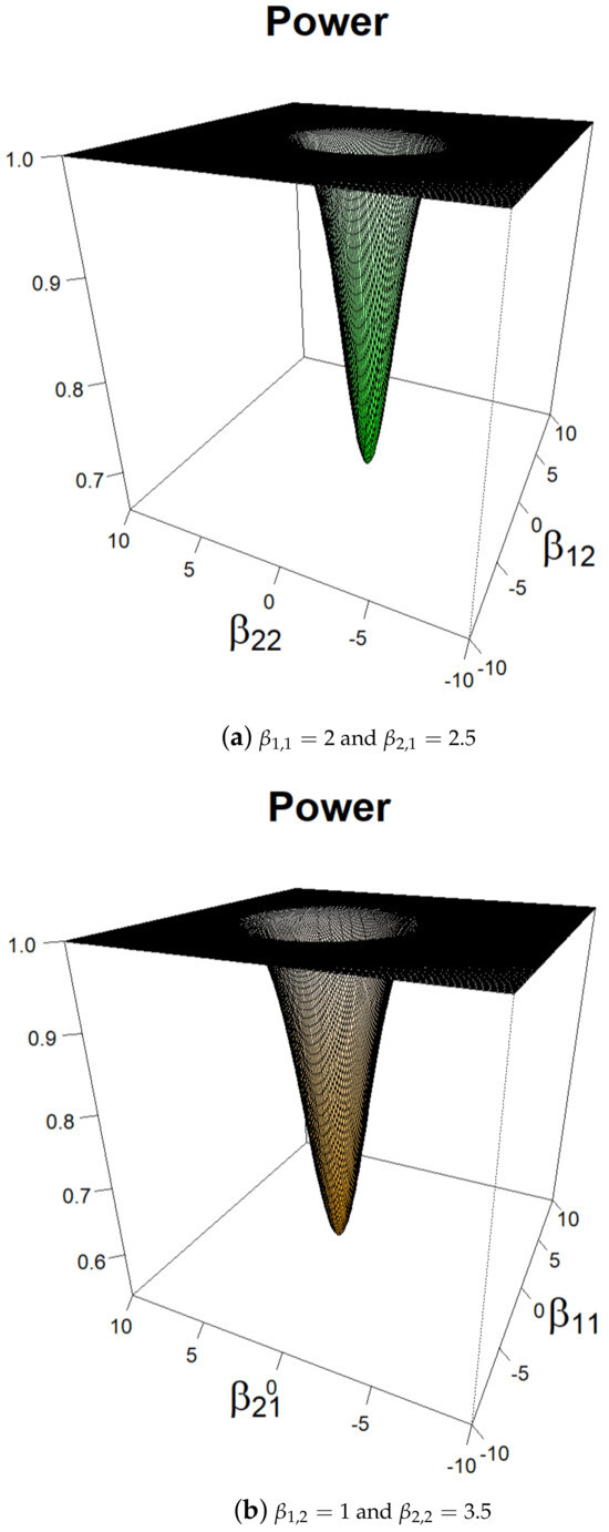
Figure 1. Power of the test with respect to $\beta$ in a class of AR(1) models when f is a standard Gaussian density.

5.2.2. ${\gamma }_0$ and f Are Unknown

As we said before, in practice, ${\mathit{\gamma }}_0$ and f are unknown and must be estimated. While we estimated ${\mathit{\gamma }}_0$ by the least-squares method, we estimate f by the Parzen–Rosenbatt estimator (see [30]), defined by

$$\begin{array}{c}\hfill {\widehat{f}}_n\left(x\right)={\displaystyle \frac{1}{n{h}_n^2}}\sum _{t=1}^{n}K\left({\displaystyle \frac{x-{\widehat{\epsilon }}_t}{h_n}}\right),x\in \mathbb{R},\end{array}$$

where

$$\begin{array}{c}\hfill {\widehat{\epsilon }}_t={\displaystyle \frac{X_t-T({\widehat{\mathit{\rho }}}_n+{\widehat{\gamma }}_n\odot \omega \left(t\right),{\mathbf{X}}_{t-1})}{V\left({\mathbf{X}}_{t-1}\right)}},\end{array}$$

where ${\widehat{\mathit{\rho }}}_n$ and ${\widehat{\mathit{\gamma }}}_n$ denote the least-squares estimators of ${\mathit{\rho }}_0$ and ${\mathit{\gamma }}_0$, respectively, $h_n$ is the smoothing parameter, and K the kernel symmetric function having the following properties:

1.

$K\left(x\right)>0$ for any $x\in \mathbb{R}$ (positivity).

2.

${\displaystyle {\int }_{\mathbb{R}}K\left(x\right)dx=1}$ (density).

3.

${\displaystyle {\int }_{\mathbb{R}}xK\left(x\right)dx=0}$ (by symmetry).

Now, we calculate the power of the test using these estimators. We choose a Gaussian kernel K and $h_n\sim {\sigma }_n{n}^{-\frac{1}{5}}$, with ${\sigma }_n$ being the sample standard deviation. We consider a sample of $n=100$ observations, $n_1\left(n\right)=40,n_2\left(n\right)=60$ and we generate the observations from (13). The results for ${\rho }_{0,1}=0.8,{\rho }_{0,2}=0.2,{\rho }_{0,3}=0,{\theta }_1=1$ and ${\theta }_2=0.02$ at the level of significance $5\%$ are given in Figure 2. It is clear that the local power of the test has approximately the same behavior for the standard Gaussian and the standard Student densities. The results do not change significantly for Epanechnikov, uniform kernel, quadratic kernel, etc.

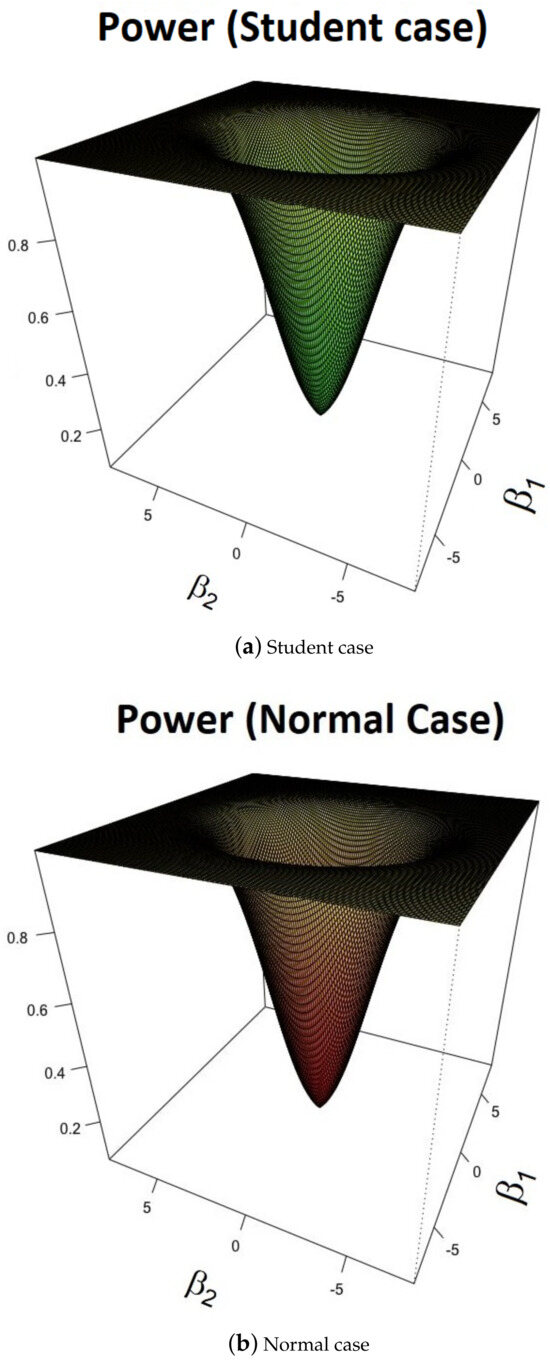
Figure 2. Power of the test with respect to $\beta$ in a class of AR(1) model when f is the kernel estimated.

5.3. Detection of Change Points and Estimation of Their Locations

In this subsection, we detect change points and we estimate their locations in simulated data. Ref. [4] studied the case of changes only in ${\rho }_{0,1}$. We start by evaluating the power of the test in case of no break in the data. Next, we study changes in ${\rho }_{0,2}$. Finally, we study changes in ${\rho }_{0,1}$ and ${\rho }_{0,2}$ simultaneously.

5.3.1. No Break

Following the algorithm in Section 4, we start by calculating the asymptotic local power given by (7) in the case where there is no break, that is, for $k=0$. We consider a sample of $n=200$ observations generated from Model (13), for ${\mathit{\gamma }}_0=0$ and f, a standard Gaussian density.

For ${\rho }_{0,1}=0.5,{\rho }_{0,2}={\rho }_{0,3}={\theta }_2=0$ and ${\theta }_1=1$, the asymptotic local power of our test with different levels of significance is plotted on Figure 3. We can see there that the local power does not exceed $0.1012$ when $\alpha =10\%$ and does not exceed $0.0507$ when $\alpha =5\%$. Then, for any $\alpha =5\%,$ or $10\%$, for the thresholds corresponding to $\zeta =0.002$ and $0.0008$, respectively, we keep the null hypothesis and conclude that there is no break in the data.

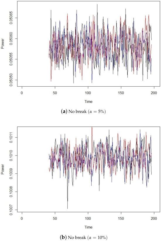
Figure 3. No break in the data.

5.3.2. Case of One Single Break

Here, we consider the problem of detecting one single break when it happens jointly in ${\rho }_{0,1}$ and ${\rho }_{0,2}$. For $\alpha =5\%,n=200,{\rho }_{0,1}=0.5,{\rho }_{0,2}=-0.2$ and ${\rho }_{0,3}={\beta }_{1,3}=0$, for different values of ${\tau }_1$ and ${\mathit{\beta }}_1=({\beta }_{1,1},{\beta }_{1,2})$; the estimation of the break location, as well as the root mean square error (RMSE), is presented in Table 1. One can see from this table that the estimation is accurate and that the RMSE is large for smaller $\left|\right|\beta \left|\right|$.

Table 1. Break location in an AR(1) model with the corresponding RMSE.

${\mathit{\tau }}_1$	$\left(\begin{array}{c}{\mathit{\beta }}_{1,1}\\ {\mathit{\beta }}_{1,2}\end{array}\right)$
	$\left(\begin{array}{c}\mathbf{2}\\ \mathbf{1}\end{array}\right)$	$\left(\begin{array}{c}\mathbf{1}\\ \mathbf{2}\end{array}\right)$	$\left(\begin{array}{c}-\mathbf{2}\\ \mathbf{1}\end{array}\right)$	$\left(\begin{array}{c}-\mathbf{2}\\ \mathbf{3}\end{array}\right)$	$\left(\begin{array}{c}-\mathbf{3}\\ \mathbf{2}\end{array}\right)$
80	78 (4.32)	81 (1.41)	82 (4.01)	80 (0.654)	80 (0.34)
100	99 (6.96)	99 (4.67)	102 (3.34)	101 (1.23)	100 (0.54)
120	122 (5.12)	121 (2.32)	119 (2.45)	120 (0.23)	121 (1.23)
140	143 (10.24)	142 (2.22)	141 (2.35)	140 (0.22)	141 (1.12)
160	164 (11.65)	164 (4.43)	162 (2.23)	161 (1.32)	161 (1.12)
185	188 (8.21)	189 (5.32)	190 (6.33)	190 (7.43)	189 (8.23)

5.4. Case of Three Breaks ($k=3$)

Now, we study the case of three breaks when piece-wise models AR(1) and AR(1)-ARCH(1) are adjusted to the data. Note that these models are sub-classes of CHARN(1,1) models.

5.4.1. AR(1) Models

We start with AR(1) models. For $\tau =({\tau }_1,{\tau }_2,{\tau }_3),$ the data are obtained from (13); for $j=1,2,3$, ${\rho }_{0,3}={\beta }_{j,3}=0$, ${\theta }_2=0$, ${\theta }_1=1$, and $\left({\epsilon }_t\right)$ is a sequence of standard Gaussian white noise. The number of change points is assumed to be unknown, and we aim to detect them and estimate their locations using our theoretical results and following our algorithm. For 5000 replications, $n=400,{\mathit{\rho }}_0=({\rho }_{0,1},{\rho }_{0,2})=(0.2,0.3),$ $\tau =({\tau }_1,{\tau }_2,{\tau }_3)=(90,190,275)$, for different values of the magnitude of change ${\mathit{\beta }}_j={({\beta }_{j,1},{\beta }_{j,2})}^{\top },j=1,2,3$, and for the same threshold $\zeta =0.1\%$, the estimations obtained are displayed in Table 2 together with their associated RMSE (in brackets). These results seem to show that our method tends to estimate the correct number of changes but overestimates their locations with a relatively large RMSE when the jumps in the parameters of the AR(1) models are too small. Again for an AR(1) model, for $j=1,2,3$, we fix ${\mathit{\beta }}_j={((3,2),(1,3),(-1,1))}^{\top }$, and the instants of breaks $\tau =(90,190,275)$, and we monitor the corresponding break estimates with respect to the variation in the threshold corresponding to different $\zeta$. For $\zeta =0.07\%$, our method overestimates the number of changes (six instants detected). For $\zeta =0.1\%$ and $0.15\%$, it estimates the correct number of changes but overestimates their locations. For $\zeta =0.25\%$, it underestimates the number of changes and overestimates their locations. The overestimation of the break locations may be explained by the weakness of the magnitude of changes. If we consider the same study for $\mathit{\beta }={((5,3),(-1-2),(4,6))}^{\top }$, we obtain the same results for the number of changes, but with more accurate change location estimations.

Table 2. Break location estimation in a class of AR(1) models for a fixed $\zeta$.

$({\mathit{\beta }}_1,{\mathit{\beta }}_2,{\mathit{\beta }}_3)$	$\mathit{\tau }=({\mathit{\tau }}_1,{\mathit{\tau }}_2,{\mathit{\tau }}_3)=(90,190,275)$ and $\mathbf{\zeta }=\mathbf{0}.\mathbf{1}$
$\begin{array}{c}\\ \left(\begin{array}{ccc}\left[\begin{array}{c}3\\ \\ 2\end{array}\right]& ,\left[\begin{array}{c}1\\ \\ 3\end{array}\right]& ,\left[\begin{array}{c}-1\\ \\ 1\end{array}\right]\end{array}\right)\end{array}$	(93,193,277) (5.78)
$\begin{array}{c}\\ \left(\begin{array}{ccc}\left[\begin{array}{c}1\\ \\ -0.5\end{array}\right]& ,\left[\begin{array}{c}2\\ \\ 1\end{array}\right]& ,\left[\begin{array}{c}-1\\ \\ -1\end{array}\right]\end{array}\right)\end{array}$	(93,194,278) (9.87)
$\begin{array}{c}\\ \left(\begin{array}{ccc}\left[\begin{array}{c}-2\\ \\ 1.5\end{array}\right]& ,\left[\begin{array}{c}1\\ \\ 3\end{array}\right]& ,\left[\begin{array}{c}-0.5\\ \\ -1\end{array}\right]\end{array}\right)\end{array}$	(92,193,277) (8.99)

5.4.2. AR(1)-ARCH(1) Models

Here, we consider Model (13) for ${\rho }_{0,1}=0.2,{\rho }_{0,2}=0.3$, ${\mathit{\beta }}_1={(3,-2)}^{\top },{\mathit{\beta }}_2={(1,1)}^{\top },{\mathit{\beta }}_3={(-2,4)}^{\top }$, ${\theta }_1=1$, ${\theta }_2=0.02$ and ${\rho }_{0,3}={\beta }_{j,3}=0$, $j=1,2,3$, which leads to an AR(1)-ARCH(1) model. For $n=350,$ Table 3 shows the estimation of change locations corresponding to the same $\zeta$ and different magnitudes of change. We can see that our method estimates the correct number of changes but overestimates their locations with a relatively large RMSE.

Table 3. Break location estimation in AR-ARCH models.

$({\mathit{\beta }}_1,{\mathit{\beta }}_2,{\mathit{\beta }}_3)$	$\mathit{\tau }=({\mathit{\tau }}_1,{\mathit{\tau }}_2,{\mathit{\tau }}_3)=(90,190,275)$ and  $\mathbf{\zeta }=\mathbf{0}.\mathbf{1}$
$\begin{array}{c}\\ \left(\begin{array}{ccc}\left[\begin{array}{c}3\\ \\ 2\end{array}\right]& ,\left[\begin{array}{c}1\\ \\ 3\end{array}\right]& ,\left[\begin{array}{c}-1\\ \\ 1\end{array}\right]\end{array}\right)\end{array}$	(93,193,277) (9.43)
$\begin{array}{c}\\ \left(\begin{array}{ccc}\left[\begin{array}{c}1\\ \\ -0.5\end{array}\right]& ,\left[\begin{array}{c}2\\ \\ 1\end{array}\right]& ,\left[\begin{array}{c}-1\\ \\ -1\end{array}\right]\end{array}\right)\end{array}$	(93,194,278) (10.64)
$\begin{array}{c}\\ \left(\begin{array}{ccc}\left[\begin{array}{c}-2\\ \\ 1.5\end{array}\right]& ,\left[\begin{array}{c}1\\ \\ 3\end{array}\right]& ,\left[\begin{array}{c}-0.5\\ \\ -1\end{array}\right]\end{array}\right)\end{array}$	(92,193,277) (6.10)

5.4.3. Conclusions

Based on the previous simulation results, we can conclude that our method is sensitive to the choice of $\zeta$, and is efficient in detecting weak changes and estimating their locations in an AR(1)-ARCH(1) model we have considered when the magnitudes of the changes are not too small.

5.5. Comparison with [27]

In a class of shifted models, Ref. [28] performed a comparison between her method, which is a different case from ours, and other methods including the one of [27]. She concluded that her method is more efficient for estimating weak break locations.

In this section, we compare our method to that of [27], denoted by SCUSUM, for a class of more general models. Recalling Model (13), we consider many cases of one single break corresponding to different instants ${\tau }_1$, and we take ${\rho }_{0,3}={\beta }_{1,3}={\theta }_2=0$ and ${\theta }_1=1$. For $n=200,$ $\alpha =5\%,{\rho }_{0,1}=0.5$, ${\rho }_{0,2}=-0.2$ and different values of ${\mathit{\beta }}_1=({\beta }_{1,1},{\beta }_{1,2})$ we perform 1000 replications, and at each replication, the change location is estimated by SCUSUM and by our method. Table 4 shows the results obtained.

Table 4. Break location estimation obtained by our method and SCUSUM for different instants of break ${\tau }_1$ and different magnitudes of change.

${\mathit{\tau }}_1=80$	$\left(\begin{array}{c}{\mathit{\beta }}_{1,1}\\ {\mathit{\beta }}_{1,2}\end{array}\right)$
	$\left(\begin{array}{c}\mathbf{2}\\ \mathbf{1}\end{array}\right)$	$\left(\begin{array}{c}\mathbf{1}\\ \mathbf{2}\end{array}\right)$	$\left(\begin{array}{c}-\mathbf{2}\\ \mathbf{1}\end{array}\right)$	$\left(\begin{array}{c}-\mathbf{2}\\ \mathbf{3}\end{array}\right)$	$\left(\begin{array}{c}-\mathbf{3}\\ \mathbf{2}\end{array}\right)$
Our method	83	81	82	80	80
SCUSUM	95	99	86	122	99
${\tau }_1=120$
Our method	122	121	121	120	121
SCUSUM	110	114	105	125	122
${\tau }_1=185$
Our method	189	188	186	186	185
SCUSUM	105	103	122	114	101

For most of the 1000 replications, SCUSUM was not able to detect any change. For that reason, we kept only the cases where it detected a change, and we calculatec the mean of the change locations estimated. The results are displayed in Table 4, from which it is obvious that our method is more accurate than SCUSUM for the detection of weak changes in the parameters of the AR(1) model studied.

5.6. Application to Real Data

Here, we applied our methodology to detecting changes in the log S&P stock price data obtained from the website https://finance.yahoo.com/quote/, accessed on 1 May 2024. These daily data cover the period from January 1992 to December 2000 and represent one of the most closely followed stock market indices worldwide, serving as a significant indicator of the U.S. economy. The raw data exhibit a trend, which shows that the S&P 500 index is non-stationary (see Figure 4). With this, our methodology can not be directly applied to this series.

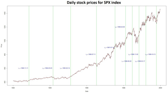
Figure 4. Estimated change points in the S&P 500 indices.

Let $P_t$ denote the S&P 500 stock price index on day t, and define $X_t$ as

$$X_t=log\left(\frac{P_t}{P_{t-1}}\right)$$

The function log being monotonic implies that the change-point locations in $\left(P_t\right)$, $(log\left(P_t\right))$, and $\left(X_t\right)$ are identical. Graphically (refer to Figure 5), $X_t$ appears to be approximately piece-wise stationary over a finite number of segments, which aligns with the requirements for applying our methodology to study changes in the raw data.

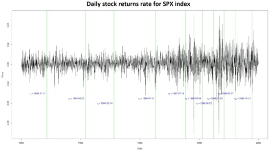
Figure 5. Estimated change points in the residual series of S&P 500 indices.

To accommodate these characteristics, we adjust the CHARN model $X_t={\beta }_j/\sqrt{n}+{\theta }_j{\epsilon }_t$ within each segment $[{\tau }_j,{\tau }_{j+1})$, where ${\epsilon }_t\sim \mathcal{N}(0,1)$. The Gaussian assumption is validated by applying the Shapiro–Wilk test.

Then, applying our procedure to this model, we obtained the following break location dates: 1992-11-11, 1994-03-03, 1995-02-14, 1996-07-11, 1997-07-14, 1998-02-09, 1998-06-22, 1998-11-02, 1999-03-17, and 1999-10-13. The changes occurring in 1992 can be linked to the damage caused by the hurricane Andrew or by the Europian Monetary System crisis. The one in 1994 can be associated with the U.S. lifting of the trade embargo on Vietnam. Those in 1995 can be due to the bankruptcy of the Barings bank. That in 1997 may be associated with the Asian crisis. Those in 1998 may be connected to the rescue organized by the New York Federal Reverve Bank. Finally, those of 1999 can be associated with the cancellation of the 1933 Glass–Steagall Act by the so-called Grammi–Leachi–Bliley Act.

6. Conclusions

We generalized the work of [4] to a class of more general CHARN models. We studied weak breaks in the parameters of the function T when the function V and the parameters ${\mathit{\rho }}_0$ and ${\mathit{\gamma }}_0$ are known. We established a LAN and contiguity results. We given an explicit expression of the local power of the test.

Next, we studied the case where ${\mathit{\rho }}_0$ is unknown and ${\mathit{\gamma }}_0$ is known or unknown. We estimated these parameters, and proved the convergence of the central sequence based on the estimated parameters to the one based on the true parameters. In this case, we proved that the test remains optimal if we replace the parameters with their estimators. From these results, we used the theoretical power for detecting weak breaks and estimating their locations in time series through an algorithm that we constructed.

The simulation experiment conducted shows that our method can detect weak breaks in the parameters of the linear AR(1) and the non-linear AR(1)-ARCH(1) models considered. Also, the location of the breaks as well as their number can be accurately estimated when the magnitudes are not too small.

Compared to [27], it seems to be more efficient for estimating weak break locations. Sometimes, the method in [27] detects breaks in data simulated with no break. This did not happen with our method when we chose a suitable $\zeta$. Our method was also applied to a set of financial data.

Appendix A.1. Proof of Theorem 1

For any $\mathit{\beta }\in {\mathbb{R}}^{p(k+1)}$, the log-likelihood ratio of $H_0$ against $H_{\mathit{\beta }}^{\left(n\right)}$ is given by

$$\begin{array}{c}\hfill {\displaystyle {\Theta }_n({\mathit{\rho }}_0,{\mathit{\gamma }}_0,\mathit{\beta })=\sum _{t=1}^n\left\{log\left[f\left({\epsilon }_t({\mathit{\rho }}_0,{\mathit{\gamma }}_n)\right)\right]-log\left[f\left({\epsilon }_t({\mathit{\rho }}_0,{\mathit{\gamma }}_0)\right)\right]\right\}.}\end{array}$$

(A1)

First, we show that as $n\to +\infty$, ${\Theta }_n({\mathit{\rho }}_0,{\mathit{\gamma }}_0,\mathit{\beta })$ decomposes into

$$\begin{array}{c}\hfill {\Theta }_n({\mathit{\rho }}_0,{\mathit{\gamma }}_0,\mathit{\beta })={\mathrm{\Pi }}_n-{\Delta }_n+o_P\left(1\right),\end{array}$$

where

$$\begin{array}{ccc}\hfill {\Delta }_n& =& {\displaystyle {\displaystyle \frac{1}{2n}}\sum _{t=1}^n\{{\displaystyle \frac{1}{V^2\left({\mathbf{X}}_{t-1}\right)}}{\mathit{\beta }}^{\top }M({\mathit{\gamma }}_0,{\mathbf{X}}_{t-1})\mathit{\beta }{\varphi }_f^{\prime }\left[{\epsilon }_t({\mathit{\rho }}_0,{\mathit{\gamma }}_0)\right]}\hfill \end{array}$$

$$\begin{array}{ccc}& & -{\displaystyle \frac{1}{V\left({\mathbf{X}}_{t-1}\right)}}{\mathit{\beta }}^{\top }\mathcal{H}({\mathit{\gamma }}_0,{\mathbf{X}}_{t-1})\mathit{\beta }{\varphi }_f\left[{\epsilon }_t({\mathit{\rho }}_0,{\mathit{\gamma }}_0)\right]\},\hfill \end{array}$$

(A2)

$$\begin{array}{ccc}\hfill {\mathrm{\Pi }}_n& =& {\displaystyle \frac{1}{\sqrt{n}}}\sum _{t=1}^n\left\{{\displaystyle \frac{1}{V\left({\mathbf{X}}_{t-1}\right)}}{\mathit{\beta }}^{\top }N({\mathit{\gamma }}_0,{\mathbf{X}}_{t-1}){\varphi }_f\left[{\epsilon }_t({\mathit{\rho }}_0,{\mathit{\gamma }}_0)\right]\right\},\hfill \end{array}$$

(A3)

and

• $N(\mathit{\gamma },{\mathbf{X}}_{t-1})={\left({\omega }_1\left(t\right){\partial }_{{\mathit{\gamma }}_1}\left[T({\mathit{\rho }}_0,\mathit{\gamma },{\mathbf{X}}_{t-1})\right],\dots ,{\omega }_{k+1}\left(t\right){\partial }_{{\mathit{\gamma }}_{k+1}}\left[T({\mathit{\rho }}_0,\mathit{\gamma },{\mathbf{X}}_{t-1})\right]\right)}^{\top }\in {\mathbb{R}}^{p(k+1)},$ and for $i=1,\dots ,k+1,$ ${\omega }_i\in \{0,1\}$,
• ${\displaystyle M(\mathit{\gamma },{\mathbf{X}}_{t-1})=\left(\begin{array}{cccc}{M}_1(\mathit{\gamma },{\mathbf{X}}_{t-1})& \mathbf{0}& \dots & \mathbf{0}\\ \mathbf{0}& M_2(\mathit{\gamma },{\mathbf{X}}_{t-1})& \ddots & ⋮\\ ⋮& \ddots & \ddots & \mathbf{0}\\ \mathbf{0}& \dots & \mathbf{0}& M_{k+1}(\mathit{\gamma },{\mathbf{X}}_{t-1})\end{array}\right)\in {\mathcal{M}}_{p(k+1)}\left(\mathbb{R}\right),}$ where $\mathbf{0}\in {\mathcal{M}}_p\left(\mathbb{R}\right)$ is a null matrix and for any $i=1,\dots ,k+1,$

  $$\begin{array}{cc}\hfill & M_i(\mathit{\gamma },{\mathbf{X}}_{t-1})={\omega }_i^2\left(t\right)\hfill \\ \hfill & \left(\begin{array}{ccc}{\displaystyle \frac{\partial T}{\partial {\gamma }_{i,1}}}({\mathit{\rho }}_0,\mathit{\gamma },{\mathbf{X}}_{t-1}){\displaystyle \frac{\partial T}{\partial {\gamma }_{i,1}}}({\mathit{\rho }}_0,\mathit{\gamma },{\mathbf{X}}_{t-1})& \dots & {\displaystyle \frac{\partial T}{\partial {\gamma }_{i,1}}}({\mathit{\rho }}_0,\mathit{\gamma },{\mathbf{X}}_{t-1}){\displaystyle \frac{\partial T}{\partial {\gamma }_{i,p}}}({\mathit{\rho }}_0,\mathit{\gamma },{\mathbf{X}}_{t-1})\\ ⋮& \ddots & ⋮\\ {\displaystyle \frac{\partial T}{\partial {\gamma }_{i,p}}}({\mathit{\rho }}_0,\mathit{\gamma },{\mathbf{X}}_{t-1}){\displaystyle \frac{\partial T}{\partial {\gamma }_{i,1}}}({\mathit{\rho }}_0,\mathit{\gamma },{\mathbf{X}}_{t-1})& \dots & {\displaystyle \frac{\partial T}{\partial {\gamma }_{i,p}}}({\mathit{\rho }}_0,\mathit{\gamma },{\mathbf{X}}_{t-1}){\displaystyle \frac{\partial T}{\partial {\gamma }_{i,p}}}({\mathit{\rho }}_0,\mathit{\gamma },{\mathbf{X}}_{t-1})\end{array}\right)\hfill \\ & \in {\mathcal{M}}_p\left(\mathbb{R}\right),\hfill \end{array}$$
• $\mathcal{H}(\mathit{\gamma },{\mathbf{X}}_{t-1})=\left(\begin{array}{cccc}{\mathcal{H}}_1(\mathit{\gamma },{\mathbf{X}}_{t-1})& \mathbf{0}& \dots & \mathbf{0}\\ \mathbf{0}& {\mathcal{H}}_2(\mathit{\gamma },{\mathbf{X}}_{t-1})& \ddots & ⋮\\ ⋮& \ddots & \ddots & \mathbf{0}\\ \mathbf{0}& \dots & \mathbf{0}& {\mathcal{H}}_{k+1}(\mathit{\gamma },{\mathbf{X}}_{t-1})\end{array}\right)\in {\mathcal{M}}_{p(k+1)}\left(\mathbb{R}\right),$ where, for $i=1,\dots ,k+1$,
  ${\mathcal{H}}_i(\mathit{\gamma },{\mathbf{X}}_{t-1})={\omega }_i^2\left(t\right)\left(\begin{array}{ccc}{\displaystyle \frac{{\partial }^{2}T}{\partial {\gamma }_{i,1}^2}}({\mathit{\rho }}_0,\mathit{\gamma },{\mathbf{X}}_{t-1})& \dots & {\displaystyle \frac{{\partial }^{2}T}{\partial {\gamma }_{i,p}\partial {\gamma }_{i,1}}}({\mathit{\rho }}_0,\mathit{\gamma },{\mathbf{X}}_{t-1})\\ ⋮& \ddots & ⋮\\ {\displaystyle \frac{{\partial }^{2}T}{\partial {\gamma }_{i,1}\partial {\gamma }_{i,p}}}({\mathit{\rho }}_0,\mathit{\gamma },{\mathbf{X}}_{t-1})& \dots & {\displaystyle \frac{{\partial }^{2}T}{\partial {\gamma }_{i,p}^2}}({\mathit{\rho }}_0,\mathit{\gamma },{\mathbf{X}}_{t-1})\end{array}\right)\in {\mathcal{M}}_p\left(\mathbb{R}\right).$

Applying a first-order Taylor expansion on $log\left\{f\left[{\epsilon }_t({\mathit{\rho }}_0,\mathit{\gamma })\right]\right\}$ in a neighborhood of ${\mathit{\gamma }}_0$, we obtain, for some $\tilde{\mathit{\gamma }}$ lying between ${\mathit{\gamma }}_0$ and ${\mathit{\gamma }}_n$,

$$\begin{array}{cc}\hfill & log\left\{f\left[{\epsilon }_t\left({\mathit{\rho }}_0,{\mathit{\gamma }}_n\right)\right]\right\}-log\left\{f\left[{\epsilon }_t\left({\mathit{\rho }}_0,{\mathit{\gamma }}_0\right)\right]\right\}={\left({\mathit{\gamma }}_n-{\mathit{\gamma }}_0\right)}^{\top }\left(D_{\mathit{\gamma }}[log\left(f\left\{{\epsilon }_t\left(\mathit{\gamma }\right)\right\}\right)]\right){|}_{\gamma ={\mathit{\gamma }}_0}\hfill \\ \hfill +& {\displaystyle \frac{1}{2}}{\left({\mathit{\gamma }}_n-{\mathit{\gamma }}_0\right)}^{\top }{H}_{\mathit{\gamma }}\left[log\left(f\left\{{\epsilon }_t\left(\mathit{\gamma }\right)\right\}\right)\right]{|}_{\gamma =\tilde{\mathit{\gamma }}}\left({\mathit{\gamma }}_n-{\mathit{\gamma }}_0\right).\hfill \end{array}$$

To simplify the study, we calculate all the expressions we need.

• $D_{\mathit{\gamma }}\left[{\epsilon }_t({\mathit{\rho }}_0,\mathit{\gamma })\right]=-{\displaystyle \frac{1}{V\left({\mathbf{X}}_{t-1}\right)}}N(\mathit{\gamma },{\mathbf{X}}_{t-1}),$
• $H_{\mathit{\gamma }}\left[{\epsilon }_t({\mathit{\rho }}_0,\mathit{\gamma })\right]=-{\displaystyle \frac{1}{V\left({\mathbf{X}}_{t-1}\right)}}{H}_{\mathit{\gamma }}\left[T({\mathit{\rho }}_0,\mathit{\gamma },{\mathbf{X}}_{t-1})\right],$
• $\begin{array}{cc}{D}_{\mathit{\gamma }}\left[log\left(f\left\{{\epsilon }_t({\mathit{\rho }}_0,\mathit{\gamma })\right\}\right)\right]& ={\displaystyle \frac{1}{V\left({\mathbf{X}}_{t-1}\right)}}N(\mathit{\gamma },{\mathbf{X}}_{t-1}){\varphi }_f\left[{\epsilon }_t({\mathit{\rho }}_0,\mathit{\gamma })\right]\hfill \\ & =-D_{\mathit{\gamma }}\left[{\epsilon }_t({\mathit{\rho }}_0,\mathit{\gamma })\right]{\varphi }_f\left[{\epsilon }_t({\mathit{\rho }}_0,\mathit{\gamma })\right],\hfill \end{array}$
• $\begin{array}{cc}{H}_{\mathit{\gamma }}\left(log\left\{f\left[{\epsilon }_t({\mathit{\rho }}_0,\mathit{\gamma })\right]\right\}\right)& =-{\displaystyle \frac{1}{V^2\left({\mathbf{X}}_{t-1}\right)}}M(\mathit{\gamma },{\mathbf{X}}_{t-1}){\varphi }_f^{\prime }\left[{\epsilon }_t({\mathit{\rho }}_0,\mathit{\gamma })\right]\hfill \\ & +{\displaystyle \frac{1}{V\left({\mathbf{X}}_{t-1}\right)}}{H}_{\mathit{\gamma }}\left[T({\mathit{\rho }}_0,\mathit{\gamma },{\mathbf{X}}_{t-1})\right]{\varphi }_f\left[{\epsilon }_t({\mathit{\rho }}_0,\mathit{\gamma })\right]\hfill \\ & =-{\displaystyle \frac{1}{V^2\left({\mathbf{X}}_{t-1}\right)}}M(\mathit{\gamma },{\mathbf{X}}_{t-1}){\varphi }_f^{\prime }\left[{\epsilon }_t({\mathit{\rho }}_0,\mathit{\gamma })\right]\hfill \\ & -H_{\mathit{\gamma }}\left[{\epsilon }_t({\mathit{\rho }}_0,\mathit{\gamma })\right]{\varphi }_f\left[{\epsilon }_t({\mathit{\rho }}_0,\mathit{\gamma })\right].\hfill \end{array}$

Then,

$$\begin{array}{cc}\hfill & log\left\{f\left[{\epsilon }_t\left({\mathit{\rho }}_0,{\mathit{\gamma }}_n\right)\right]\right\}-log\left\{f\left[{\epsilon }_t\left({\mathit{\rho }}_0,{\mathit{\gamma }}_0\right)\right]\right\}={\displaystyle \frac{1}{\sqrt{n}}}{\displaystyle \frac{{\mathit{\beta }}^{\top }N({\mathit{\gamma }}_0,{\mathbf{X}}_{t-1})}{V\left({\mathbf{X}}_{t-1}\right)}}{\varphi }_f\left[{\epsilon }_t({\mathit{\rho }}_0,{\mathit{\gamma }}_0)\right]\hfill \\ \hfill & -{\displaystyle \frac{1}{2n}}\left[{\displaystyle \frac{1}{V^2\left({\mathbf{X}}_{t-1}\right)}}{\mathit{\beta }}^{\top }M(\tilde{\mathit{\gamma }},{\mathbf{X}}_{t-1})\mathit{\beta }{\varphi }_f^{\prime }\left[{\epsilon }_t({\mathit{\rho }}_0,\tilde{\mathit{\gamma }})\right]\right]\hfill \\ \hfill & -{\displaystyle \frac{1}{2n}}\left[{\displaystyle \frac{1}{V\left({\mathbf{X}}_{t-1}\right)}}{\mathit{\beta }}^{\top }{H}_{\mathit{\gamma }}\left[T({\mathit{\rho }}_0,\tilde{\mathit{\gamma }},{\mathbf{X}}_{t-1})\right]\mathit{\beta }{\varphi }_f\left[{\epsilon }_t({\mathit{\rho }}_0,\tilde{\mathit{\gamma }})\right]\right].\hfill \end{array}$$

Now,

$$\begin{array}{cc}\hfill {\displaystyle {\Theta }_n({\mathit{\rho }}_0,{\mathit{\gamma }}_0,\mathit{\beta })}& ={\displaystyle \frac{1}{\sqrt{n}}}\sum _{t=1}^n{\displaystyle \frac{1}{V\left({\mathbf{X}}_{t-1}\right)}}{\mathit{\beta }}^{\top }N({\mathit{\gamma }}_0,{\mathbf{X}}_{t-1}){\varphi }_f\left[{\epsilon }_t({\mathit{\rho }}_0,{\mathit{\gamma }}_0)\right]\hfill \\ \hfill & -{\displaystyle \frac{1}{2n}}\sum _{t=1}^n{\displaystyle \frac{1}{V^2\left({\mathbf{X}}_{t-1}\right)}}{\mathit{\beta }}^{\top }M(\tilde{\mathit{\gamma }},{\mathbf{X}}_{t-1})\mathit{\beta }{\varphi }_f^{\prime }\left[{\epsilon }_t({\mathit{\rho }}_0,\tilde{\mathit{\gamma }})\right]\hfill \\ & +{\displaystyle \frac{1}{2n}}\sum _{t=1}^n{\displaystyle \frac{1}{V\left({\mathbf{X}}_{t-1}\right)}}{\mathit{\beta }}^{\top }\mathcal{H}(\tilde{\mathit{\gamma }},{\mathbf{X}}_{t-1})\mathit{\beta }{\varphi }_f\left[{\epsilon }_t({\mathit{\rho }}_0,\tilde{\mathit{\gamma }})\right],\hfill \end{array}$$

where, observing that for any t and for any $i\ne j$, ${\omega }_i\left(t\right){\omega }_j\left(t\right)=0,$

$$\begin{array}{c}\hfill {\displaystyle M(\tilde{\mathit{\gamma }},{\mathbf{X}}_{t-1})=\left(\begin{array}{cccc}{M}_1(\tilde{\mathit{\gamma }},{\mathbf{X}}_{t-1})& \mathbf{0}& \dots & \mathbf{0}\\ \mathbf{0}& M_2(\tilde{\mathit{\gamma }},{\mathbf{X}}_{t-1})& \ddots & ⋮\\ ⋮& \ddots & \ddots & \mathbf{0}\\ \mathbf{0}& \dots & \mathbf{0}& M_{k+1}(\tilde{\mathit{\gamma }},{\mathbf{X}}_{t-1})\end{array}\right)\in {\mathcal{M}}_{p(k+1)}\left(\mathbb{R}\right),}\end{array}$$

with $\mathbf{0}\in {\mathcal{M}}_p\left(\mathbb{R}\right)$ standing for a null matrix and

$$\begin{array}{cc}\hfill & M_i(\tilde{\mathit{\gamma }},{\mathbf{X}}_{t-1})=\hfill \\ & {\omega }_i^2\left(t\right)\left(\begin{array}{ccc}{\displaystyle \frac{\partial T}{\partial {\gamma }_{i,1}}}({\mathit{\rho }}_0,\tilde{\mathit{\gamma }},{\mathbf{X}}_{t-1}){\displaystyle \frac{\partial T}{\partial {\gamma }_{i,1}}}({\mathit{\rho }}_0,\tilde{\mathit{\gamma }},{\mathbf{X}}_{t-1})& \dots & {\displaystyle \frac{\partial T}{\partial {\gamma }_{i,1}}}({\mathit{\rho }}_0,\tilde{\mathit{\gamma }},{\mathbf{X}}_{t-1}){\displaystyle \frac{\partial T}{\partial {\gamma }_{i,p}}}({\mathit{\rho }}_0,\tilde{\mathit{\gamma }},{\mathbf{X}}_{t-1})\\ ⋮& \ddots & ⋮\\ {\displaystyle \frac{\partial T}{\partial {\gamma }_{i,p}}}({\mathit{\rho }}_0,\tilde{\mathit{\gamma }},{\mathbf{X}}_{t-1}){\displaystyle \frac{\partial T}{\partial {\gamma }_{i,1}}}({\mathit{\rho }}_0,\tilde{\mathit{\gamma }},{\mathbf{X}}_{t-1})& \dots & {\displaystyle \frac{\partial T}{\partial {\gamma }_{i,p}}}({\mathit{\rho }}_0,\tilde{\mathit{\gamma }},{\mathbf{X}}_{t-1}){\displaystyle \frac{\partial T}{\partial {\gamma }_{i,p}}}({\mathit{\rho }}_0,\tilde{\mathit{\gamma }},{\mathbf{X}}_{t-1})\end{array}\right)\hfill \\ & \in {\mathcal{M}}_p\left(\mathbb{R}\right),\hfill \end{array}$$

$$\begin{array}{cc}\hfill \mathcal{H}(\tilde{\mathit{\gamma }},{\mathbf{X}}_{t-1})=& \left(\begin{array}{cccc}{\mathcal{H}}_1(\tilde{\mathit{\gamma }},{\mathbf{X}}_{t-1})& \mathbf{0}& \dots & \mathbf{0}\\ \mathbf{0}& {\mathcal{H}}_2(\tilde{\mathit{\gamma }},{\mathbf{X}}_{t-1})& \ddots & ⋮\\ ⋮& \ddots & \ddots & \mathbf{0}\\ \mathbf{0}& \dots & \mathbf{0}& {\mathcal{H}}_{k+1}(\tilde{\mathit{\gamma }},{\mathbf{X}}_{t-1})\end{array}\right)\in {\mathcal{M}}_{p(k+1)}\left(\mathbb{R}\right),\hfill \end{array}$$

with

$$\begin{array}{c}\hfill {\mathcal{H}}_i(\tilde{\mathit{\gamma }},{\mathbf{X}}_{t-1})={\omega }_i^2\left(t\right)\left(\begin{array}{ccc}{\displaystyle \frac{{\partial }^{2}T}{\partial {\gamma }_{i,1}^2}}({\mathit{\rho }}_0,\tilde{\mathit{\gamma }},{\mathbf{X}}_{t-1})& \dots & {\displaystyle \frac{{\partial }^{2}T}{\partial {\gamma }_{i,p}\partial {\gamma }_{i,1}}}({\mathit{\rho }}_0,\tilde{\mathit{\gamma }},{\mathbf{X}}_{t-1})\\ ⋮& \ddots & ⋮\\ {\displaystyle \frac{{\partial }^{2}T}{\partial {\gamma }_{i,1}\partial {\gamma }_{i,p}}}({\mathit{\rho }}_0,\tilde{\mathit{\gamma }},{\mathbf{X}}_{t-1})& \dots & {\displaystyle \frac{{\partial }^{2}T}{\partial {\gamma }_{i,p}^2}}({\mathit{\rho }}_0,\tilde{\mathit{\gamma }},{\mathbf{X}}_{t-1})\end{array}\right)\in {\mathcal{M}}_p\left(\mathbb{R}\right).\end{array}$$

Let

$$\begin{array}{cc}\hfill \chi (\tilde{\mathit{\gamma }},{\mathbf{X}}_{t-1})& =-{\displaystyle \frac{1}{2n}}\sum _{t=1}^n{\displaystyle \frac{1}{V^2\left({\mathbf{X}}_{t-1}\right)}}{\mathit{\beta }}^{\top }M(\tilde{\mathit{\gamma }},{\mathbf{X}}_{t-1})\mathit{\beta }{\varphi }_f^{\prime }\left[{\epsilon }_t({\mathit{\rho }}_0,\tilde{\mathit{\gamma }})\right]\hfill \\ \hfill & +{\displaystyle \frac{1}{2n}}\sum _{t=1}^n{\displaystyle \frac{1}{V\left({\mathbf{X}}_{t-1}\right)}}{\mathit{\beta }}^{\top }\left(\mathcal{H}(\tilde{\mathit{\gamma }},{\mathbf{X}}_{t-1})\right)\mathit{\beta }{\varphi }_f\left[{\epsilon }_t({\mathit{\rho }}_0,\tilde{\mathit{\gamma }})\right].\hfill \end{array}$$

Using (A₃), we have $\mathbb{E}\left\{{\varphi }_f\left[{\epsilon }_t({\mathit{\rho }}_0,\mathit{\gamma })\right]\right\}=0$, $\mathbb{E}\left\{{\varphi }_f^{\prime }\left[{\epsilon }_t({\mathit{\rho }}_0,\mathit{\gamma })\right]\right\}=I\left(f\right)$ and $\mathbb{E}\left\{\right|{\varphi }_f\left[{\epsilon }_t({\mathit{\rho }}_0,\mathit{\gamma })\right]\left|\right\}<\infty$. Now, using (A₄) and the ergodic theorem, from a simple calculation, we can prove that

$$\begin{array}{c}\hfill \left|\chi (\tilde{\mathit{\gamma }},{\mathbf{X}}_{t-1})-\chi ({\mathit{\gamma }}_0,{\mathbf{X}}_{t-1})\right|\underset{n\to +\infty }{\overset{\mathbb{P}}{\to }}0.\end{array}$$

It results from above that

$$\begin{array}{c}\hfill {\Theta }_n({\mathit{\rho }}_0,{\mathit{\gamma }}_0,\mathit{\beta })={\mathrm{\Pi }}_n-{\Delta }_n+o_P\left(1\right),\end{array}$$

where ${\Delta }_n$ and ${\mathrm{\Pi }}_n$ are defined by (A2) and (A3), respectively.

Now, we study of the asymptotic behavior of ${\Delta }_n$ under $H_0$.

By the piecewise stationarity and ergodicity, for any $j=1,\dots ,k+1$, we can write, almost surely,

$$\begin{array}{cc}\hfill \underset{n\to +\infty }{lim}{\Delta }_n& {\displaystyle ={\displaystyle \frac{1}{2}}\sum _{j=1}^{k+1}{\alpha }_j\sum _{1\le h\le m\le p}{\beta }_{j,h}{\beta }_{j,m}{\eta }_{j,2}^{(h,m)}({\mathit{\rho }}_0,{\mathit{\gamma }}_0)={\displaystyle \frac{\eta ({\mathit{\rho }}_0,{\mathit{\gamma }}_0,\mathit{\beta })}{2}},}\hfill \end{array}$$

with

$$\begin{array}{cc}\hfill {\eta }_{j,2}^{(h,m)}({\mathit{\rho }}_0,{\mathit{\gamma }}_0)& =I\left(f\right){\int }_{{\mathbb{R}}^d}{\displaystyle \frac{1}{V^2\left(x\right)}}{\displaystyle \frac{\partial T}{\partial {\gamma }_{j,h}}}({\mathit{\rho }}_0,{\mathit{\gamma }}_0,x){\displaystyle \frac{\partial T}{\partial {\gamma }_{j,m}}}({\mathit{\rho }}_0,{\mathit{\gamma }}_0,x)d{F}_j\left(x\right).\hfill \end{array}$$

Thus, we can write

$$\begin{array}{c}\hfill {\Theta }_n={\mathrm{\Pi }}_n-{\displaystyle \frac{\eta ({\mathit{\rho }}_0,{\mathit{\gamma }}_0,\mathit{\beta })}{2}}+o_P\left(1\right).\end{array}$$

Now, we prove that under $H_0$,

$${\mathrm{\Pi }}_n\stackrel{\mathcal{D}}{⟶}\mathcal{N}(0,\eta ({\mathit{\rho }}_0,{\mathit{\gamma }}_0,\mathit{\beta })).$$

We consider the sequence

$$\begin{array}{cc}\hfill {\Theta }_{n,j}& ={\displaystyle \frac{1}{\sqrt{n}}}\sum _{t=1}^j{\displaystyle \frac{1}{V\left({\mathbf{X}}_{t-1}\right)}}{\mathit{\beta }}^{\top }N({\mathit{\gamma }}_0,{\mathbf{X}}_{t-1}){\varphi }_f\left[{\epsilon }_t({\mathit{\rho }}_0,{\mathit{\gamma }}_0)\right],j=1,\dots ,n,\hfill \end{array}$$

and we define for every $t=1,\dots ,n,$

$$\begin{array}{c}\hfill {\psi }_{n,t}={\displaystyle \frac{1}{\sqrt{n}}}{\displaystyle \frac{1}{V\left({\mathbf{X}}_{t-1}\right)}}{\mathit{\beta }}^{\top }N({\mathit{\gamma }}_0,{\mathbf{X}}_{t-1}){\varphi }_f\left[{\epsilon }_t({\mathit{\rho }}_0,{\mathit{\gamma }}_0)\right].\end{array}$$

We use Corollary 3.1 of [31] to study the asymptotic behavior of ${\Theta }_{n,j}$.

It is easy to prove that $\left\{\right({\Theta }_{n,j},{\mathcal{F}}_j),j=1,\dots ,n$ is a martingale sequence.

Using the fact that ${\epsilon }_t$ is independent of ${\mathcal{F}}_{t-1}$ for $t=1,\dots ,n$ and using the ergodic theorem, we can show that, almost surely,

$$\begin{array}{cc}\hfill {\displaystyle \underset{n\to +\infty }{lim}\sum _{t=1}^n\mathbb{E}\left({\psi }_{n,t}^2\right|{\mathcal{F}}_{t-1})}& =\sum _{j=1}^{k+1}{\alpha }_j\sum _{1\le h\le m\le p}{\beta }_{j,h}{\beta }_{j,m}{\eta }_{j,2}^{(h,m)}({\mathit{\rho }}_0,{\mathit{\gamma }}_0)=\eta ({\mathit{\rho }}_0,{\mathit{\gamma }}_0,\mathit{\beta })\hfill \\ \hfill & <\infty ,\hfill \end{array}$$

which shows that the first condition of Corollary 3.1 of [31] is verified. It remains to check the Linderberg condition. Let $ϵ>0$; by the Hölder inequality, using Markov inequality and the ergodic theorem, we can write that as $n\to \infty$,

$$\begin{array}{cc}\hfill {\displaystyle \sum _{t=1}^n\mathbb{E}\left({\psi }_{n,t}^2{\mathbf{1}}_{|{\psi }_{n,t}|>ϵ}\right|{\mathcal{F}}_{t-1})}& \stackrel{a.s}{\to }0.\hfill \end{array}$$

Then, the conditions of Corollary 3.1 of [31] are completely verified, so that under $H_0$, we have

$$\begin{array}{c}\hfill {\mathrm{\Pi }}_n({\mathit{\rho }}_0,{\mathit{\gamma }}_0,\mathit{\beta })\stackrel{\mathcal{D}}{⟶}\mathcal{N}(0,\eta ({\mathit{\rho }}_0,{\mathit{\gamma }}_0,\mathit{\beta })).\end{array}$$

(A4)

Consequently, under $H_0$, we have

$$\begin{array}{c}\hfill {\Theta }_n({\mathit{\rho }}_0,{\mathit{\gamma }}_0,\mathit{\beta })\stackrel{\mathcal{D}}{⟶}\mathcal{N}\left(-{\displaystyle \frac{\eta ({\mathit{\rho }}_0,{\mathit{\gamma }}_0,\mathit{\beta })}{2}},\eta ({\mathit{\rho }}_0,{\mathit{\gamma }}_0,\mathit{\beta })\right).\end{array}$$

(A5)

Collecting the above results, the LAN property is established with the central sequence ${\mathrm{\Pi }}_n({\mathit{\rho }}_0,{\mathit{\gamma }}_0,\mathit{\beta })$.

Appendix A.2. Proof of Corollary 1

For any $\mathit{\beta }\in {\mathbb{R}}^{p(k+1)}$, from Theorem 1, under $H_0$, as $n\to +\infty ,$

$$\begin{array}{c}\hfill {\mathrm{\Pi }}_n({\mathit{\rho }}_0,{\mathit{\gamma }}_0,\mathit{\beta })\stackrel{\mathcal{D}}{⟶}\mathcal{N}(0,\eta ({\mathit{\rho }}_0,{\mathit{\gamma }}_0,\mathit{\beta })).\end{array}$$

It results that, under $H_0$, as $n\to +\infty$,

$$\begin{array}{c}\hfill {\Theta }_n({\mathit{\rho }}_0,{\mathit{\gamma }}_0,\mathit{\beta })\stackrel{\mathcal{D}}{⟶}\mathcal{N}\left(-{\displaystyle \frac{\eta ({\mathit{\rho }}_0,{\mathit{\gamma }}_0,\mathit{\beta })}{2}},\eta ({\mathit{\rho }}_0,{\mathit{\gamma }}_0,\mathit{\beta })\right).\end{array}$$

Then, it is easy to see that under $H_0,$ as $n\to +\infty$,

$$\begin{array}{cc}\hfill {\displaystyle \left(\begin{array}{c}{\mathrm{\Pi }}_n({\mathit{\gamma }}_0,\mathit{\beta })\\ {\Theta }_n({\mathit{\rho }}_0,{\mathit{\gamma }}_0,\mathit{\beta })\end{array}\right)}& \stackrel{\mathcal{D}}{⟶}\mathcal{N}\left(\begin{array}{c}\left(\begin{array}{c}0\\ -{\displaystyle \frac{\eta ({\mathit{\rho }}_0,{\mathit{\gamma }}_0,\mathit{\beta })}{2}}\end{array}\right),\left(\begin{array}{cc}\eta ({\mathit{\rho }}_0,{\mathit{\gamma }}_0,\mathit{\beta })& {\sigma }_{1,2}\\ {\sigma }_{2,1}& \eta ({\mathit{\rho }}_0,{\mathit{\gamma }}_0,\mathit{\beta })\end{array}\right)\end{array}\right),\hfill \end{array}$$

where ${\displaystyle {\sigma }_{1,2}={\sigma }_{2,1}=\underset{n\to +\infty }{lim}\mathbb{C}ov({\mathrm{\Pi }}_n,{\Theta }_n)=\underset{n\to +\infty }{lim}\left[\mathbb{E}\left({\mathrm{\Pi }}_n{\Theta }_n\right)-\mathbb{E}\left({\mathrm{\Pi }}_n\right)\mathbb{E}\left({\Theta }_n\right)\right]}$.

Since $\mathbb{E}\left({\mathrm{\Pi }}_n\right)=0$ and

$$\begin{array}{cc}\hfill \underset{n\to +\infty }{lim}\mathbb{E}\left({\Theta }_n{\mathrm{\Pi }}_n\right)& =\underset{n\to +\infty }{lim}\left[\mathbb{E}\left({\mathrm{\Pi }}_n^2\right)-\mathbb{E}\left({\mathrm{\Pi }}_n{\Delta }_n\right)\right]=\eta ({\mathit{\rho }}_0,{\mathit{\gamma }}_0,\mathit{\beta }),\hfill \end{array}$$

under $H_0$, we have

$$\begin{array}{cc}\hfill {\displaystyle \left(\begin{array}{c}{\mathrm{\Pi }}_n({\mathit{\rho }}_0,{\mathit{\gamma }}_0,\mathit{\beta })\\ {\Theta }_n\end{array}\right)}& \stackrel{\mathcal{D}}{⟶}\mathcal{N}\left(\begin{array}{c}\left(\begin{array}{c}0\\ -{\displaystyle \frac{\eta ({\mathit{\rho }}_0,{\mathit{\gamma }}_0,\mathit{\beta })}{2}}\end{array}\right),\left(\begin{array}{cc}\eta ({\mathit{\rho }}_0,{\mathit{\gamma }}_0,\mathit{\beta })& \eta ({\mathit{\rho }}_0,{\mathit{\gamma }}_0,\mathit{\beta })\\ \eta ({\mathit{\rho }}_0,{\mathit{\gamma }}_0,\mathit{\beta })& \eta ({\mathit{\rho }}_0,{\mathit{\gamma }}_0,\mathit{\beta })\end{array}\right)\end{array}\right).\hfill \end{array}$$

(A6)

Using [32] or [33], we obtain that the sequences $\{H_{\mathit{\beta }}^{\left(n\right)}:n\ge 1\}$ and $\{H_0^{\left(n\right)}=H_0:n\ge 1\}$ are contiguous, and that under $H_{\mathit{\beta }}^{\left(n\right)}$, as $n\to +\infty$,

$$\begin{array}{c}\hfill {\mathrm{\Pi }}_n({\mathit{\rho }}_0,{\mathit{\gamma }}_0,\mathit{\beta })\stackrel{\mathcal{D}}{\to }\mathcal{N}(\eta ({\mathit{\rho }}_0,{\mathit{\gamma }}_0,\mathit{\beta }),\eta ({\mathit{\rho }}_0,{\mathit{\gamma }}_0,\mathit{\beta })).\end{array}$$

Appendix A.3. Proof of Theorem 2

From Theorem 1 and Corollary 1, we can conclude immediately that, under $H_0$, as $n\to +\infty$,

$$\begin{array}{cc}\hfill {\displaystyle \left(\begin{array}{c}{\mathrm{\Pi }}_n({\mathit{\rho }}_0,{\mathit{\gamma }}_0,\mathit{\beta })\\ {\Theta }_n\end{array}\right)}& \stackrel{\mathcal{D}}{⟶}\mathcal{N}\left(\begin{array}{c}\left(\begin{array}{c}0\\ -{\displaystyle \frac{\eta ({\mathit{\rho }}_0,{\mathit{\gamma }}_0,\mathit{\beta })}{2}}\end{array}\right),\left(\begin{array}{cc}\eta ({\mathit{\rho }}_0,{\mathit{\gamma }}_0,\mathit{\beta })& \eta ({\mathit{\rho }}_0,{\mathit{\gamma }}_0,\mathit{\beta })\\ \eta ({\mathit{\rho }}_0,{\mathit{\gamma }}_0,\mathit{\beta })& \eta ({\mathit{\rho }}_0,{\mathit{\gamma }}_0,\mathit{\beta })\end{array}\right)\end{array}\right).\hfill \end{array}$$

(A7)

Part [i] is a direct consequence of Theorem 2 and is briefly explained in the proof of Corollary 1.

As explained there, the sequences of hypotheses are contiguous, and under $H_{\mathit{\beta }}^{\left(n\right)}$, as $n\to +\infty$, we have

$$\begin{array}{c}\hfill {\mathrm{\Pi }}_n({\mathit{\rho }}_0,{\mathit{\gamma }}_0,\mathit{\beta })\stackrel{\mathcal{D}}{⟶}\mathcal{N}(\eta ({\mathit{\rho }}_0,{\mathit{\gamma }}_0,\mathit{\beta }),\eta ({\mathit{\rho }}_0,{\mathit{\gamma }}_0,\mathit{\beta })).\end{array}$$

By (A6) and the Le Cam’s third lemma (Proposition 4.2 in [32]), under $H_{\mathit{\beta }}^{\left(n\right)}$, as $n\to +\infty$,

$$\begin{array}{c}\hfill {\mathrm{\Pi }}_n({\mathit{\rho }}_0,{\mathit{\gamma }}_0,\mathit{\beta })\stackrel{\mathcal{D}}{⟶}\mathcal{N}(\eta ({\mathit{\rho }}_0,{\mathit{\gamma }}_0,\mathit{\beta }),\eta ({\mathit{\rho }}_0,{\mathit{\gamma }}_0,\mathit{\beta })).\end{array}$$

We recall that, under $H_0$, as $n\to +\infty$,

$${\widehat{\vartheta }}_n({\mathit{\rho }}_0,{\mathit{\gamma }}_0,\mathit{\beta })⟶\vartheta ({\mathit{\rho }}_0,{\mathit{\gamma }}_0,\mathit{\beta }),$$

where $\vartheta ({\mathit{\rho }}_0,{\mathit{\gamma }}_0,\mathit{\beta })=\sqrt{\eta ({\mathit{\rho }}_0,{\mathit{\gamma }}_0,\mathit{\beta })}.$

This convergence remains true under $H_{\mathit{\beta }}^{\left(n\right)}$ by contiguity. From Theorem 2, it can be seen that, as $n\to +\infty$, under $H_0$,

$$\begin{array}{c}\hfill {\mathcal{T}}_n({\mathit{\rho }}_0,{\mathit{\gamma }}_0,\mathit{\beta })\stackrel{\mathcal{D}}{⟶}\mathcal{N}(0,1).\end{array}$$

Thus, by the Le Cam’s third lemma, we can conclude that under $H_{\mathit{\beta }}^{\left(n\right)}$, as $n\to +\infty$,

$$\begin{array}{c}\hfill {\displaystyle \frac{{\mathrm{\Pi }}_n({\mathit{\rho }}_0,{\mathit{\gamma }}_0,\mathit{\beta })}{{\widehat{\vartheta }}_n({\mathit{\rho }}_0,{\mathit{\gamma }}_0,\mathit{\beta })}}\stackrel{\mathcal{D}}{⟶}\mathcal{N}(\vartheta ({\mathit{\rho }}_0,{\mathit{\gamma }}_0,\mathit{\beta }),1).\end{array}$$

Indeed, for $n\ge 1$, we can write

$$\begin{array}{c}\hfill {\displaystyle \frac{{\mathrm{\Pi }}_n({\mathit{\rho }}_0,{\mathit{\gamma }}_0,\mathit{\beta })}{{\widehat{\vartheta }}_n({\mathit{\rho }}_0,{\mathit{\gamma }}_0,\mathit{\beta })}}={\displaystyle \frac{{\mathrm{\Pi }}_n({\mathit{\rho }}_0,{\mathit{\gamma }}_0,\mathit{\beta })}{\vartheta ({\mathit{\rho }}_0,{\mathit{\gamma }}_0,\mathit{\beta })}}\times {\displaystyle \frac{\vartheta ({\mathit{\rho }}_0,{\mathit{\gamma }}_0,\mathit{\beta })}{{\widehat{\vartheta }}_n({\mathit{\rho }}_0,{\mathit{\gamma }}_0,\mathit{\beta })}}.\end{array}$$

From which it results that, under $H_{\mathit{\beta }}^{\left(n\right)}$ and as $n\to +\infty$,

$$\begin{array}{c}\hfill {\displaystyle \frac{{\mathrm{\Pi }}_n({\mathit{\rho }}_0,{\mathit{\gamma }}_0,\mathit{\beta })}{\vartheta ({\mathit{\rho }}_0,{\mathit{\gamma }}_0,\mathit{\beta })}}\stackrel{\mathcal{D}}{⟶}\mathcal{N}(\vartheta ({\mathit{\rho }}_0,{\mathit{\gamma }}_0,\mathit{\beta }),1).\end{array}$$

For parts [ii] and [iii], to calculate the asymptotic power of our test statistic, we calculate the asymptotic cumulative distribution of ${\displaystyle \frac{{\mathrm{\Pi }}_n({\mathit{\rho }}_0,{\mathit{\gamma }}_0,\mathit{\beta })}{{\widehat{\vartheta }}_n({\mathit{\rho }}_0,{\mathit{\gamma }}_0,\mathit{\beta })}}$ under $H_{\mathit{\beta }}^{\left(n\right)}$. We have

$$\begin{array}{cc}\hfill \underset{n\to +\infty }{lim}P\left({\displaystyle \frac{{\mathrm{\Pi }}_n({\mathit{\rho }}_0,{\mathit{\gamma }}_0,\mathit{\beta })}{{\widehat{\vartheta }}_n({\mathit{\rho }}_0,{\mathit{\gamma }}_0,\mathit{\beta })}}>z_{\alpha }|H_{\mathit{\beta }}^{\left(n\right)}\right)& =\underset{n\to +\infty }{lim}P\left({\displaystyle \frac{{\mathrm{\Pi }}_n({\mathit{\rho }}_0,{\mathit{\gamma }}_0,\mathit{\beta })}{\vartheta ({\mathit{\rho }}_0,{\mathit{\gamma }}_0,\mathit{\beta })}}>z_{\alpha }|H_{\mathit{\beta }}^{\left(n\right)}\right)\hfill \\ \hfill & =1-\mathrm{\Phi }(z_{\alpha }-\vartheta ({\mathit{\rho }}_0,{\mathit{\gamma }}_0,\mathit{\beta }))\hfill \\ \hfill & ={\mathcal{P}}_{k,{\tau }^k},\hfill \end{array}$$

(A8)

where $\mathrm{\Phi }$ is the cumulative distribution function of a standard Gaussian law with $z_{\alpha }$ its $(1-\alpha )$-quantile.

By Section 4.4.3 of [33], the test based on ${\mathcal{T}}_n({\mathit{\rho }}_0,{\mathit{\gamma }}_0,\mathit{\beta })$ is locally asymptotically optimal.

Appendix A.4. Proof of Proposition 1

Appendix A.4.1. Proof of [i]

From the Bahadur representation (9), as in [34,35], we consider the following sequence:

$$\begin{array}{c}\hfill {\displaystyle R_{n,j}=n^{-\frac{1}{2}}\sum _{t=1}^j{\rm Y}({\mathit{\rho }}_0,{\mathbf{X}}_{t-1})\aleph \left[{\epsilon }_t({\mathit{\rho }}_0,{\mathit{\gamma }}_0)\right],j=1,\dots ,n.}\end{array}$$

and

$$\begin{array}{cc}\hfill & u^{\top }{R}_{n,j}={\displaystyle \frac{1}{\sqrt{n}}}\sum _{t=1}^j{y}_t\left(u\right)\in \mathbb{R},\mathrm{where}{y}_t\left(u\right)=u^{\top }{\rm Y}({\mathit{\rho }}_0,{\mathbf{X}}_{t-1})\aleph \left[{\epsilon }_t({\mathit{\rho }}_0,{\mathit{\gamma }}_0)\right],\hfill \\ & u\in {\mathbb{R}}^p.\hfill \end{array}$$

It is easy to see that $u^{\top }{R}_{n,j}$ is centered for every $j=1,\dots ,n$. Since $\mathbb{E}\{\aleph \left[{\epsilon }_t({\mathit{\rho }}_0,{\mathit{\gamma }}_0)\right]\}=0$ for any $t\in \mathbb{N}$, from a simple calculation, we prove that $\{(u^{\top }{R}_{n,j},{\mathcal{F}}_j),j=1,\dots ,n\}$ is a martingale sequence.

We check now the first condition of Corollary 3.1 of [31]. Since ${\epsilon }_t$ is independent of ${\mathcal{F}}_{t-1}$ for $t=1,\dots ,n,$ we can write

$$\begin{array}{cc}\hfill & \sum _{t=1}^n\mathbb{E}\left\{{\left[n^{-\frac{1}{2}}{y}_t\left(u\right)\right]}^2|{\mathcal{F}}_{t-1}\right\}\hfill \\ \hfill & =\sum _{t=1}^n{n}^{-1}\mathbb{E}\left\{{\left[u^{\top }{\rm Y}({\mathit{\rho }}_0,{\mathbf{X}}_{t-1})\aleph \left[{\epsilon }_t({\mathit{\rho }}_0,{\mathit{\gamma }}_0)\right]\right]}^2|{\mathcal{F}}_{t-1}\right\}\hfill \\ \hfill & =\sum _{j=1}^{k+1}{\displaystyle \frac{n_j\left(n\right)}{n}}{\displaystyle \frac{1}{n_j\left(n\right)}}\sum _{t={\tau }_{j-1}}^{{\tau }_j}{\left[u^{\top }{\rm Y}({\mathit{\rho }}_0,{\mathbf{X}}_{t-1})\right]}^2\mathbb{E}\left\{{\aleph }^2\left[{\epsilon }_t({\mathit{\rho }}_0,{\mathit{\gamma }}_0)\right]\right\}.\hfill \end{array}$$

By the assumptions (${\mathcal{B}}_2$), (${\mathcal{B}}_3$) and the ergodic theorem, for $j=1,\dots ,k+1$, we can write

$$\begin{array}{cc}\hfill {\displaystyle \frac{1}{n_j\left(n\right)}}\sum _{t={\tau }_{j-1}}^{{\tau }_j}{\left[u^{\top }{\rm Y}({\mathit{\rho }}_0,{\mathbf{X}}_{t-1})\right]}^2\mathbb{E}\left\{{\aleph }^2\left[{\epsilon }_t({\mathit{\rho }}_0,{\mathit{\gamma }}_0)\right]\right\}\stackrel{a.s.}{\to }& {\int }_{{\mathbb{R}}^d}{\left[u^{\top }{\rm Y}({\mathit{\rho }}_0,x)\right]}^{2}d{F}_j\left(x\right)\hfill \\ & \times {\int }_{\mathbb{R}}{\aleph }^2\left(x\right)f\left(x\right)dx<\infty .\hfill \end{array}$$

Then,

$$\begin{array}{cc}\hfill \sum _{t=1}^n\mathbb{E}\left\{{\left[{\displaystyle \frac{1}{\sqrt{n}}}{y}_t\left(u\right)\right]}^2\right|{\mathcal{F}}_{t-1}\}\underset{n\to +\infty }{\overset{a.s.}{\to }}s& ={\int }_{\mathbb{R}}{\aleph }^2\left(x\right)f\left(x\right)dx\hfill \\ \hfill & \times \sum _{j=1}^{k+1}{\alpha }_j{\int }_{{\mathbb{R}}^d}{\left[u^{\top }{\rm Y}({\mathit{\rho }}_0,x)\right]}^{2}d{F}_j\left(x\right).\hfill \end{array}$$

Finally, we check the Linderberg condition, that is, the second condition of Corollary 3.1 of [31]. In this purpose, we prove that, as n $\to +\infty$,

$$\begin{array}{c}\hfill \sum _{t=1}^n\mathbb{E}\left\{{\left[n^{-\frac{1}{2}}{y}_t\left(u\right)\right]}^2{\mathbf{1}}_{\left|n^{-\frac{1}{2}}{y}_t\left(u\right)\right|>ϵ}|{\mathcal{F}}_{t-1}\right\}\stackrel{a.s.}{\to }0.\end{array}$$

Let $ϵ>0$. By the Hölder inequality, and Markov inequalities, we can write

$$\begin{array}{cc}\hfill & \sum _{t=1}^n\mathbb{E}\left\{{\left[n^{-\frac{1}{2}}{y}_t\left(u\right)\right]}^2{\mathbf{1}}_{\left|n^{-\frac{1}{2}}{y}_t\left(u\right)\right|>ϵ}|{\mathcal{F}}_{t-1}\right\}\hfill \\ \hfill & \le \sum _{t=1}^n{\mathbb{E}}^{\frac{2}{3}}\left\{{\left[n^{-\frac{1}{2}}{y}_t\left(u\right)\right]}^3|{\mathcal{F}}_{t-1}\right\}{\mathbb{E}}^{\frac{1}{3}}\left\{{\mathbf{1}}_{\left|n^{-\frac{1}{2}}{y}_t\left(u\right)\right|>ϵ}|{\mathcal{F}}_{t-1}\right\}\hfill \\ \hfill & \le \sum _{t=1}^n{\mathbb{E}}^{\frac{2}{3}}\left\{{\left[n^{-\frac{1}{2}}{y}_t\left(u\right)\right]}^3|{\mathcal{F}}_{t-1}\right\}{\displaystyle \frac{{\mathbb{E}}^{\frac{1}{3}}\left\{{\left|n^{-\frac{1}{2}}{y}_t\left(u\right)\right|}^3>ϵ|{\mathcal{F}}_{t-1}\right\}}{\sqrt[3]{ϵ}}}\hfill \\ \hfill & \le {\displaystyle \frac{1}{\sqrt[3]{ϵ}\sqrt{n}}}\sum _{j=1}^{k+1}{\displaystyle \frac{n_j\left(n\right)}{n}}{\displaystyle \frac{1}{n_j\left(n\right)}}\sum _{t={\tau }_{j-1}}^{{\tau }_j}{\parallel u^{\top }{\rm Y}({\mathit{\rho }}_0,{\mathbf{X}}_{t-1})\parallel }^3\mathbb{E}\left\{|\aleph \left[{\epsilon }_t({\mathit{\rho }}_0,{\mathit{\gamma }}_0)\right]{|}^3\right\}.\hfill \end{array}$$

By the piece-wise stationarity and the ergodic theorem, for $j=1,\dots ,k+1$, we obtain almost surely that

$$\begin{array}{cc}\hfill & \underset{n\to +\infty }{lim}{\displaystyle \frac{1}{\sqrt{n}}}\sum _{j=1}^{k+1}{\displaystyle \frac{n_j\left(n\right)}{n}}\left({\displaystyle \frac{1}{n_j\left(n\right)}}\sum _{t={\tau }_{j-1}}^{{\tau }_j}{\parallel u^{\top }{\rm Y}({\mathit{\rho }}_0,{\mathbf{X}}_{t-1})\parallel }^3\mathbb{E}\left\{|\aleph \left[{\epsilon }_t({\mathit{\rho }}_0,{\mathit{\gamma }}_0)\right]{|}^3\right\}\right)=0\hfill \end{array}$$

Then, using Corollary 3.1 of [31], we conclude that, under $H_0$, we have

$$\begin{array}{c}\hfill u^{\top }\sqrt{n}({\mathit{\rho }}_{\mathbf{n}}-{\mathit{\rho }}_0)\stackrel{\mathcal{D}}{\to }\mathcal{N}(0,u^{\top }\mathrm{\Sigma }u).\end{array}$$

which implies that, under $H_0$ and as $n\to +\infty$,

$$\begin{array}{c}\hfill \sqrt{n}({\mathit{\rho }}_{\mathbf{n}}-{\mathit{\rho }}_0)\stackrel{\mathcal{D}}{\to }\mathcal{N}(0,\mathrm{\Sigma })\end{array}$$

where $\mathrm{\Sigma }$ is the covariance matrix defined as

$$\begin{array}{c}\hfill \mathrm{\Sigma }={\int }_{\mathbb{R}}{\aleph }^2\left(x\right)f\left(x\right)dx\sum _{j=1}^{k+1}{\alpha }_j{\int }_{{\mathbb{R}}^d}{\rm Y}({\mathit{\rho }}_0,x){{\rm Y}}^{\top }({\mathit{\rho }}_0,x)d{F}_j\left(x\right)\in {\mathcal{M}}_p\left(\mathbb{R}\right).\end{array}$$

Appendix A.4.2. Proof of [ii]

We recall that under $H_0$, as $n\to +\infty$,

$$\begin{array}{cc}\hfill \sqrt{n}({\mathit{\rho }}_{\mathbf{n}}-{\mathit{\rho }}_0)& \stackrel{a.s.}{\to }\mathcal{N}(0,\mathrm{\Sigma }),\hfill \\ \hfill {\Theta }_n({\mathit{\rho }}_0,{\mathit{\gamma }}_0,\mathit{\beta })& \stackrel{\mathcal{D}}{\to }\mathcal{N}\left(-{\displaystyle \frac{\eta ({\mathit{\rho }}_0,{\mathit{\gamma }}_0,\mathit{\beta })}{2}},\eta ({\mathit{\rho }}_0,{\mathit{\gamma }}_0,\mathit{\beta })\right),\hfill \end{array}$$

where

$$\begin{array}{cc}\hfill \eta ({\mathit{\rho }}_0,{\mathit{\gamma }}_0,\mathit{\beta })& =\sum _{j=1}^{k+1}{\alpha }_j\sum _{1\le h\le m\le p}{\beta }_{j,h}{\beta }_{j,m}{\eta }_{j,2}^{(h,m)}({\mathit{\rho }}_0,{\mathit{\gamma }}_0),\hfill \end{array}$$

with

$$\begin{array}{cc}\hfill {\eta }_{j,2}^{(h,m)}({\mathit{\rho }}_0,{\mathit{\gamma }}_0)& =I\left(f\right){\int }_{{\mathbb{R}}^d}{\displaystyle \frac{1}{V^2\left(x\right)}}{\displaystyle \frac{\partial T}{\partial {\gamma }_{j,h}}}({\mathit{\rho }}_0,{\mathit{\gamma }}_0,x){\displaystyle \frac{\partial T}{\partial {\gamma }_{j,m}}}({\mathit{\rho }}_0,{\mathit{\gamma }}_0,x)d{F}_j\left(x\right).\hfill \end{array}$$

We consider the sequence $Q_n=\sqrt{n}({\mathit{\rho }}_{\mathbf{n}}-{\mathit{\rho }}_0)$. By Le Cam’s third lemma, under $H_0$, as $n\to +\infty$,

$$\begin{array}{c}\hfill \left(\begin{array}{c}{Q}_n\\ {\Theta }_n({\mathit{\rho }}_0,{\mathit{\gamma }}_0,\mathit{\beta })\end{array}\right)\stackrel{\mathcal{D}}{\to }\mathcal{N}\left(\left(\begin{array}{c}0\\ -{\displaystyle \frac{\eta ({\mathit{\rho }}_0,{\mathit{\gamma }}_0,\mathit{\beta })}{2}}\end{array}\right),\mathrm{\Xi }\right),\end{array}$$

where

$$\begin{array}{cc}\hfill \mathrm{\Xi }& =\underset{n\to +\infty }{lim}\left(\begin{array}{cc}\mathbb{V}ar\left(Q_n\right)& \mathbb{C}ov(Q_n,{\Theta }_n)\\ \mathbb{C}ov(Q_n,{\Theta }_n)& \mathbb{V}ar\left({\Theta }_n\right)\end{array}\right),\hfill \\ \hfill \mathbb{C}ov(Q_n,{\Theta }_n({\mathit{\rho }}_0,{\mathit{\gamma }}_0,\mathit{\beta })& =\mathbb{C}ov\left(Q_n,{\mathrm{\Pi }}_n({\mathit{\rho }}_0,{\mathit{\gamma }}_0,\mathit{\beta })-{\displaystyle \frac{\eta ({\mathit{\rho }}_0,{\mathit{\gamma }}_0,\mathit{\beta })}{2}}\right)\hfill \\ \hfill & ={\displaystyle \frac{1}{\sqrt{n}}}\sum _{t=1}^n[\mathbb{E}\left\{{\displaystyle \frac{Q_n}{V\left({\mathbf{X}}_{t-1}\right)}}{\mathit{\beta }}^{\top }N({\mathit{\gamma }}_0,{\mathbf{X}}_{t-1}){\varphi }_f\left[{\epsilon }_t({\mathit{\rho }}_0,{\mathit{\gamma }}_0)\right]\right\}\hfill \\ \hfill & -\mathbb{E}\left(Q_n\right)\mathbb{E}\left\{{\displaystyle \frac{1}{V\left({\mathbf{X}}_{t-1}\right)}}{\mathit{\beta }}^{\top }N({\mathit{\gamma }}_0,{\mathbf{X}}_{t-1})\right\}\mathbb{E}\left\{{\varphi }_f\left[{\epsilon }_t({\mathit{\rho }}_0,{\mathit{\gamma }}_0)\right]\right\}].\hfill \end{array}$$

Since $\mathbb{E}\left\{{\varphi }_f\left[{\epsilon }_t({\mathit{\rho }}_0,{\mathit{\gamma }}_0)\right]\right\}=0$, ${\displaystyle \underset{n\to +\infty }{lim}\mathbb{E}\left(Q_n\right)=0}$, ${\epsilon }_t$ is independent of ${\mathcal{F}}_{t-1}$, $\mathbb{E}\{\aleph \left[{\epsilon }_t({\mathit{\rho }}_0,{\mathit{\gamma }}_0)\right]\}=0$, and using the stationarity and the ergodic theorem, we can easily see that

$$\begin{array}{c}\hfill \mathbb{C}ov(Q_n,{\Theta }_n({\mathit{\rho }}_0,{\mathit{\gamma }}_0,\mathit{\beta })\underset{n\to +\infty }{\to }\mathcal{C},\end{array}$$

where

$$\begin{array}{c}\hfill \mathcal{C}={\int }_{\mathbb{R}}\aleph \left(x\right){\varphi }_f\left(x\right)f\left(x\right)dx\sum _{j=1}^n{\alpha }_j{\omega }_j\sum _{h=1}^p{\beta }_{j,h}{\int }_{{\mathbb{R}}^d}{\displaystyle \frac{{\rm Y}({\mathit{\rho }}_0,x)}{V\left(x\right)}}{\displaystyle \frac{\partial T}{\partial {\gamma }_{j,h}}}({\mathit{\rho }}_0,x)d{F}_j\left(x\right).\end{array}$$

Then, under $H_0$, we have

$$\begin{array}{c}\hfill \left(\begin{array}{c}{Q}_n\\ {\Theta }_n({\mathit{\rho }}_0,{\mathit{\gamma }}_0,\mathit{\beta })\end{array}\right)\stackrel{\mathcal{D}}{\to }\mathcal{N}\left(\left(\begin{array}{c}0\\ -{\displaystyle \frac{\eta ({\mathit{\rho }}_0,{\mathit{\gamma }}_0,\mathit{\beta })}{2}}\end{array}\right),\left(\begin{array}{cc}\mathrm{\Sigma }& {\mathcal{C}}^{\top }\\ \mathcal{C}& \eta ({\mathit{\rho }}_0,{\mathit{\gamma }}_0,\mathit{\beta })\end{array}\right)\right).\end{array}$$

From this result and Le Cam’s third lemma, under $H_1^{\left(n\right)}$, as n tends to $+\infty$, we have

$$\begin{array}{c}\hfill \sqrt{n}({\mathit{\rho }}_{\mathbf{n}}-{\mathit{\rho }}_0)=Q_n\stackrel{\mathcal{D}}{\to }\mathcal{N}(\mathcal{C},\mathrm{\Sigma }).\end{array}$$

Appendix A.5. Proof of Proposition 2

Appendix A.5.1. Proof of [i]

We prove the convergence of the central sequence (4) to its estimated version in order to verify that the test still be optimal when we replace the parameter by its estimator. For any $\mathit{\rho }\in {\mathbb{R}}^p$ and $\mathit{\gamma },\mathit{\beta }\in {\mathbb{R}}^{p(k+1)}$, we define

$$\begin{array}{c}\hfill {\displaystyle {\Theta }_n(\mathit{\rho },\mathit{\gamma },\mathit{\beta })=\sum _{t=1}^{n}log\left\{f\left[{\epsilon }_t\left(\mathit{\rho },\mathit{\gamma }+{\displaystyle \frac{\mathit{\beta }}{\sqrt{n}}}\right)\right]\right\}-log\left\{f\left[{\epsilon }_t(\mathit{\rho },\mathit{\gamma })\right]\right\}+o_P\left(1\right).}\end{array}$$

Then the log-likelihood ratio of $H_0$ against $H_{\mathit{\beta }}^{\left(n\right)}$ is $\Theta ({\mathit{\rho }}_0,{\mathit{\gamma }}_0,\mathit{\beta })$. For ${\tilde{\mathit{\rho }}}_n$ lying between ${\mathit{\rho }}_{\mathbf{n}}$ and ${\mathit{\rho }}_0$, we write a second-order Taylor expansion of ${\mathrm{\Pi }}_n({\mathit{\rho }}_0,{\mathit{\gamma }}_0,\mathit{\beta })$ around ${\mathit{\rho }}_{\mathbf{n}}$ and obtain

$$\begin{array}{cc}\hfill {\mathrm{\Pi }}_n({\mathit{\rho }}_0,{\mathit{\gamma }}_0,\mathit{\beta })=& {\mathrm{\Pi }}_n({\mathit{\rho }}_{\mathbf{n}},{\mathit{\gamma }}_0,\mathit{\beta })+{({\mathit{\rho }}_0-{\mathit{\rho }}_{\mathbf{n}})}^{\top }{\partial }_{\mathit{\rho }}{\mathrm{\Pi }}_n({\mathit{\rho }}_{\mathbf{n}},{\mathit{\gamma }}_0,\mathit{\beta })\hfill \\ \hfill & +\frac{1}{2}{({\mathit{\rho }}_0-{\mathit{\rho }}_{\mathbf{n}})}^{\top }{\partial }_{\mathit{\rho }}^2{\mathrm{\Pi }}_n({\tilde{\mathit{\rho }}}_n,{\mathit{\gamma }}_0,\mathit{\beta })({\mathit{\rho }}_0-{\mathit{\rho }}_{\mathbf{n}}).\hfill \end{array}$$

(A9)

We wish to prove that, under $H_0$, as $n\to +\infty$,

$$\begin{array}{cc}\hfill {({\mathit{\rho }}_0-{\mathit{\rho }}_{\mathbf{n}})}^{\top }{\partial }_{\mathit{\rho }}{\mathrm{\Pi }}_n({\mathit{\rho }}_{\mathbf{n}},{\mathit{\gamma }}_0,\mathit{\beta })& =o_P\left(1\right)\hfill \end{array}$$

(A10)

$$\begin{array}{cc}\hfill \frac{1}{2}{({\mathit{\rho }}_0-{\mathit{\rho }}_{\mathbf{n}})}^{\top }{\partial }_{\mathit{\rho }}^2{\mathrm{\Pi }}_n({\tilde{\mathit{\rho }}}_n,{\mathit{\gamma }}_0,\mathit{\beta })({\mathit{\rho }}_0-{\mathit{\rho }}_{\mathbf{n}})& =o_P\left(1\right).\hfill \end{array}$$

(A11)

In order to simplify the notations, let $T^{{\gamma }_{m,h}}=\partial T/\partial {\gamma }_{m,h}$.

$$\begin{array}{cc}\hfill & {\displaystyle \frac{1}{\sqrt{n}}}{\partial }_{\mathit{\rho }}^2{\mathrm{\Pi }}_n({\tilde{\mathit{\rho }}}_n,{\mathit{\gamma }}_0,\mathit{\beta })\hfill \\ \hfill & ={\displaystyle \frac{1}{n}}\sum _{t=1}^n{\displaystyle \frac{1}{V\left({\mathbf{X}}_{t-1}\right)}}\sum _{m=1}^{k+1}\sum _{h=1}^p{\beta }_{m,h}{\partial }_{\mathit{\rho }}^2\left(T^{{\gamma }_{m,h}}\right)({\tilde{\mathit{\rho }}}_n,{\mathit{\gamma }}_0,\mathit{\beta }){\varphi }_f\left[{\epsilon }_t({\tilde{\mathit{\rho }}}_n,{\mathit{\gamma }}_0)\right]\hfill \\ \hfill & -{\displaystyle \frac{2}{n}}\sum _{t=1}^n{\displaystyle \frac{1}{V^2\left({\mathbf{X}}_{t-1}\right)}}\sum _{m=1}^{k+1}\sum _{h=1}^p{\beta }_{m,h}{\partial }_{\mathit{\rho }}\left(T^{{\gamma }_{m,h}}\right)({\tilde{\mathit{\rho }}}_n,{\mathit{\gamma }}_0,\mathit{\beta }){\partial }_{\mathit{\rho }}^{\top }T({\tilde{\mathit{\rho }}}_n,{\mathbf{X}}_{t-1}){\varphi }_f^{\prime }\left[{\epsilon }_t({\tilde{\mathit{\rho }}}_n,{\mathit{\gamma }}_0)\right]\hfill \\ \hfill & -{\displaystyle \frac{1}{n}}\sum _{t=1}^n{\displaystyle \frac{1}{V^2\left({\mathbf{X}}_{t-1}\right)}}\sum _{m=1}^{k+1}\sum _{h=1}^p{\beta }_{m,h}{T}^{{\gamma }_{m,h}}({\tilde{\mathit{\rho }}}_n,{\mathit{\gamma }}_0,\mathit{\beta }){\partial }_{\mathit{\rho }}^{2}T({\tilde{\mathit{\rho }}}_n,{\mathbf{X}}_{t-1}){\varphi }_f^{\prime }\left[{\epsilon }_t({\tilde{\mathit{\rho }}}_n,{\mathit{\gamma }}_0)\right]\hfill \\ \hfill & +{\displaystyle \frac{1}{n}}\sum _{t=1}^n{\displaystyle \frac{1}{V^3\left({\mathbf{X}}_{t-1}\right)}}\sum _{m=1}^{k+1}\sum _{h=1}^p{\beta }_{m,h}{T}^{{\gamma }_{m,h}}({\tilde{\mathit{\rho }}}_n,{\mathit{\gamma }}_0,\mathit{\beta }){\partial }_{\mathit{\rho }}T({\tilde{\mathit{\rho }}}_n,{\mathbf{X}}_{t-1}){\partial }_{\mathit{\rho }}^{\top }T({\tilde{\mathit{\rho }}}_n,{\mathbf{X}}_{t-1})\hfill \\ \hfill & \times {\varphi }_f^{″}\left[{\epsilon }_t({\tilde{\mathit{\rho }}}_n,{\mathit{\gamma }}_0)\right]\hfill \\ \hfill & ={\Delta }_{1,n}({\tilde{\mathit{\rho }}}_n,{\mathit{\gamma }}_0,\mathit{\beta })+{\Delta }_{2,n}({\tilde{\mathit{\rho }}}_n,{\mathit{\gamma }}_0,\mathit{\beta })+{\Delta }_{3,n}({\tilde{\mathit{\rho }}}_n,{\mathit{\gamma }}_0,\mathit{\beta })+{\Delta }_{4,n}({\tilde{\mathit{\rho }}}_n,{\mathit{\gamma }}_0,\mathit{\beta }).\hfill \end{array}$$

By a multiple use of a Taylor expansion, by the assumptions (${\mathcal{B}}_4$), (A₉), by the ergodic theorem, from a simple calculation, we prove that, for $i=1,\dots ,4$, $\left|\right||{\Delta }_{i,n}({\tilde{\mathit{\rho }}}_n,{\mathit{\gamma }}_0,\mathit{\beta }){\left|\right||}_p$ is bounded.

Thus, as $n\to +\infty$, $\left(1/\sqrt{n}\right)\left|\right||{\partial }_{\mathit{\rho }}^2{\mathrm{\Pi }}_n({\tilde{\mathit{\rho }}}_n,{\mathit{\gamma }}_0,\mathit{\beta }){\left|\right||}_p$ tends in probability to a finite positive real number, denoted by b.

Recall from (A11) that, as $n\to +\infty ,$ we have

$$\begin{array}{cc}\hfill & \frac{1}{2}\left|{({\mathit{\rho }}_0-{\mathit{\rho }}_{\mathbf{n}})}^{\top }{\partial }_{\mathit{\rho }}^2{\mathrm{\Pi }}_n({\tilde{\mathit{\rho }}}_n,{\mathit{\gamma }}_0,\mathit{\beta })({\mathit{\rho }}_0-{\mathit{\rho }}_{\mathbf{n}})\right|\hfill \\ \hfill & \le \frac{1}{2}{∥\sqrt{n}({\mathit{\rho }}_0-{\mathit{\rho }}_{\mathbf{n}})∥}_p\left|\right|\left|{\displaystyle \frac{1}{\sqrt{n}}}{\partial }_{\mathit{\rho }}^2{\mathrm{\Pi }}_n({\tilde{\mathit{\rho }}}_n,{\mathit{\gamma }}_0,\mathit{\beta })\right||{|}_p{∥{\mathit{\rho }}_0-{\mathit{\rho }}_{\mathbf{n}}∥}_p\hfill \\ \hfill & \le \frac{1}{2}{∥\sqrt{n}({\mathit{\rho }}_0-{\mathit{\rho }}_{\mathbf{n}})∥}_p{∥{\mathit{\rho }}_0-{\mathit{\rho }}_{\mathbf{n}}∥}_p\times b.\hfill \end{array}$$

Since under $H_0$, as $n\to +\infty$, we have

$$\begin{array}{c}\hfill \sqrt{n}({\mathit{\rho }}_0-{\mathit{\rho }}_{\mathbf{n}})\stackrel{\mathcal{D}}{\to }\mathcal{N}(0,\mathrm{\Sigma }),\end{array}$$

it results that

$$\begin{array}{c}\hfill {\displaystyle \frac{1}{2}}{({\mathit{\rho }}_0-{\mathit{\rho }}_{\mathbf{n}})}^{\top }{\partial }_{\mathit{\rho }}^2{\mathrm{\Pi }}_n({\tilde{\mathit{\rho }}}_n,{\mathit{\gamma }}_0,\mathit{\beta })({\mathit{\rho }}_0-{\mathit{\rho }}_{\mathbf{n}})=o_P\left(1\right).\end{array}$$

(A12)

From (A12), we can write

$$\begin{array}{cc}\hfill {\mathrm{\Pi }}_n({\mathit{\rho }}_0,{\mathit{\gamma }}_0,\mathit{\beta })=& {\mathrm{\Pi }}_n({\mathit{\rho }}_{\mathbf{n}},{\mathit{\gamma }}_0,\mathit{\beta })+{({\mathit{\rho }}_0-{\mathit{\rho }}_{\mathbf{n}})}^{\top }{\partial }_{\mathit{\rho }}{\mathrm{\Pi }}_n({\mathit{\rho }}_{\mathbf{n}},{\mathit{\gamma }}_0,\mathit{\beta })+o_P\left(1\right).\hfill \end{array}$$

(A13)

Now, we prove that

$${({\mathit{\rho }}_0-{\mathit{\rho }}_{\mathbf{n}})}^{\top }{\partial }_{\mathit{\rho }}{\mathrm{\Pi }}_n({\mathit{\rho }}_{\mathbf{n}},{\mathit{\gamma }}_0,\mathit{\beta })=o_P\left(1\right).$$

Adding and subtracting appropriate terms, as $n\to +\infty$, we can write

$$\begin{array}{cc}\hfill & {\mathrm{\Pi }}_n({\mathit{\rho }}_0,{\mathit{\gamma }}_0,\mathit{\beta })\hfill \\ \hfill & ={\mathrm{\Pi }}_n({\mathit{\rho }}_{\mathbf{n}},{\mathit{\gamma }}_0,\mathit{\beta })+{({\mathit{\rho }}_0-{\mathit{\rho }}_{\mathbf{n}}+{\mathit{\rho }}_{s\left(n\right)}-{\mathit{\rho }}_{s\left(n\right)})}^{\top }{\partial }_{\mathit{\rho }}{\mathrm{\Pi }}_n({\mathit{\rho }}_{\mathbf{n}},{\mathit{\gamma }}_0,\mathit{\beta })+o_P\left(1\right)\hfill \\ \hfill & ={\mathrm{\Pi }}_n({\mathit{\rho }}_{\mathbf{n}},{\mathit{\gamma }}_0,\mathit{\beta })+{({\mathit{\rho }}_0-{\mathit{\rho }}_{s\left(n\right)})}^{\top }{\partial }_{\mathit{\rho }}{\mathrm{\Pi }}_n({\mathit{\rho }}_{\mathbf{n}},{\mathit{\gamma }}_0,\mathit{\beta })+{({\mathit{\rho }}_{s\left(n\right)}-{\mathit{\rho }}_{\mathbf{n}})}^{\top }{\partial }_{\mathit{\rho }}{\mathrm{\Pi }}_n({\mathit{\rho }}_{\mathbf{n}},{\mathit{\gamma }}_0,\mathit{\beta })\hfill \\ \hfill & +o_P\left(1\right),\hfill \end{array}$$

where ${\left\{s\left(n\right)\right\}}_{n\ge 1}$ stands for a sequence of positive integers such that $n/s\left(n\right)⟶0$ as $n\to +\infty .$

Observing that, as $n\to +\infty$,

$$\begin{array}{c}\hfill \sqrt{n}{({\mathit{\rho }}_0-{\mathit{\rho }}_{s\left(n\right)})}^{\top }=\sqrt{s\left(n\right)}{({\mathit{\rho }}_0-{\mathit{\rho }}_{s\left(n\right)})}^{\top }\times \sqrt{{\displaystyle \frac{n}{s\left(n\right)}}}=o_P\left(1\right),\end{array}$$

it is easy to see that,

$$\begin{array}{c}\hfill {({\mathit{\rho }}_0-{\mathit{\rho }}_{s\left(n\right)})}^{\top }{\partial }_{\mathit{\rho }}{\mathrm{\Pi }}_n({\mathit{\rho }}_{\mathbf{n}},{\mathit{\gamma }}_0,\mathit{\beta })=\sqrt{n}{({\mathit{\rho }}_0-{\mathit{\rho }}_{s\left(n\right)})}^{\top }{\displaystyle \frac{1}{\sqrt{n}}}{\partial }_{\mathit{\rho }}{\mathrm{\Pi }}_n({\mathit{\rho }}_{\mathbf{n}},{\mathit{\gamma }}_0,\mathit{\beta }).\end{array}$$

Then, it suffices to show that ${\partial }_{\mathit{\rho }}{\mathrm{\Pi }}_n({\mathit{\rho }}_{\mathbf{n}},{\mathit{\gamma }}_0,\mathit{\beta })/\sqrt{n}$ converges in probability to a random vector. For this, we can write the following decomposition:

$$\begin{array}{cc}\hfill & {\displaystyle \frac{1}{\sqrt{n}}}{\partial }_{\mathit{\rho }}{\mathrm{\Pi }}_n({\mathit{\rho }}_{\mathbf{n}},{\mathit{\gamma }}_0,\mathit{\beta })\hfill \\ \hfill & ={\displaystyle \frac{1}{n}}\sum _{t=1}^n{\displaystyle \frac{1}{V\left({\mathbf{X}}_{t-1}\right)}}\sum _{m=1}^{k+1}\sum _{h=1}^p{\beta }_{m,h}{\partial }_{\mathit{\rho }}\left(T^{{\gamma }_{m,h}}\right)({\mathit{\rho }}_{\mathbf{n}},{\mathit{\gamma }}_0,{\mathbf{X}}_{t-1}){\varphi }_f\left[{\epsilon }_t({\mathit{\rho }}_{\mathbf{n}},{\mathit{\gamma }}_0)\right]\hfill \\ \hfill & -{\displaystyle \frac{1}{n}}\sum _{t=1}^n{\displaystyle \frac{1}{V^2\left({\mathbf{X}}_{t-1}\right)}}\sum _{m=1}^{k+1}\sum _{h=1}^p{\beta }_{m,h}{T}^{{\gamma }_{m,h}}({\mathit{\rho }}_{\mathbf{n}},{\mathit{\gamma }}_0,{\mathbf{X}}_{t-1}){\partial }_{\mathit{\rho }}T({\mathit{\rho }}_{\mathbf{n}},{\mathit{\gamma }}_0,{\mathbf{X}}_{t-1}){\varphi }_f^{\prime }\left[{\epsilon }_t({\mathit{\rho }}_{\mathbf{n}},{\mathit{\gamma }}_0)\right]\hfill \\ \hfill & ={\mho }_{1,n}({\mathit{\rho }}_{\mathbf{n}},{\mathit{\gamma }}_0,\mathit{\beta })+{\mho }_{2,n}({\mathit{\rho }}_{\mathbf{n}},{\mathit{\gamma }}_0,\mathit{\beta }).\hfill \end{array}$$

Using the assumptions (${\mathcal{B}}_4$) and (A₅), and the ergodic theorem, since ${\epsilon }_t$ is independent of ${\mathcal{F}}_{t-1}$, the study of the asymptotic behavior of ${\mho }_{1,n}({\mathit{\rho }}_{\mathbf{n}},{\mathit{\gamma }}_0,\mathit{\beta })$ and ${\mho }_{2,n}({\mathit{\rho }}_{\mathbf{n}},{\mathit{\gamma }}_0,\mathit{\beta })$ shows that, as $n\to +\infty$,

$$\begin{array}{c}\hfill {\mho }_{1,n}({\mathit{\rho }}_{\mathbf{n}},{\mathit{\gamma }}_0,\mathit{\beta })\stackrel{\mathbb{P}}{\to }\mathbf{0}\in {\mathbb{R}}^p.\end{array}$$

Thus, ${∥{\mho }_{2,n}({\mathit{\rho }}_{\mathbf{n}},{\mathit{\gamma }}_0,\mathit{\beta })∥}_p$ tends in probability to a finite positive real number. Consequently,

$$\begin{array}{cc}\hfill {∥{\displaystyle \frac{1}{\sqrt{n}}}{\partial }_{\mathit{\rho }}{\mathrm{\Pi }}_n({\mathit{\rho }}_{\mathbf{n}},{\mathit{\gamma }}_0,\mathit{\beta })∥}_p& \le {∥{\mho }_{1,n}({\mathit{\rho }}_{\mathbf{n}},{\mathit{\gamma }}_0,\mathit{\beta })∥}_p+{∥{\mho }_{2,n}({\mathit{\rho }}_{\mathbf{n}},{\mathit{\gamma }}_0,\mathit{\beta })∥}_p<\infty .\hfill \end{array}$$

It results that

$$\begin{array}{c}\hfill {({\mathit{\rho }}_0-{\mathit{\rho }}_{s\left(n\right)})}^{\top }{\partial }_{\mathit{\rho }}{\mathrm{\Pi }}_n({\mathit{\rho }}_{\mathbf{n}},{\mathit{\gamma }}_0,\mathit{\beta })=o_P\left(1\right).\end{array}$$

Hence,

$$\begin{array}{cc}\hfill {\mathrm{\Pi }}_n({\mathit{\rho }}_0,{\mathit{\gamma }}_0,\mathit{\beta })& ={\mathrm{\Pi }}_n({\mathit{\rho }}_{\mathbf{n}},{\mathit{\gamma }}_0,\mathit{\beta })+{({\mathit{\rho }}_{s\left(n\right)}-{\mathit{\rho }}_{\mathbf{n}})}^{\top }{\partial }_{\mathit{\rho }}{\mathrm{\Pi }}_n({\mathit{\rho }}_{\mathbf{n}},{\mathit{\gamma }}_0,\mathit{\beta })+o_P\left(1\right).\hfill \end{array}$$

(A14)

In order to treat the above equation (A14), we need the following lemma.

Lemma A1.

Assume that (${\mathcal{B}}_2$) holds. Let ${\left\{s\left(n\right)\right\}}_{n\ge 1}$ be a sequence of positive integers such that $n/s\left(n\right)$ tends to 0 as $n\to +\infty$. For ${\mathit{\gamma }}_0,\mathit{\beta }\in {\mathbb{R}}^{p(k+1)}$, ${\mathit{\rho }}_{s\left(n\right)}$ is asymptotically in the tangent space ${\mathbb{T}}_n$ to the curve of ${\mathrm{\Pi }}_n(\mathit{\rho },\mathit{\gamma },\mathit{\beta })$ at ${\mathit{\rho }}_{\mathbf{n}}$, defined as follows:

$$\begin{array}{c}\hfill {\mathbb{T}}_n=\left\{z\in {\mathbb{R}}^p/{\mathrm{\Pi }}_n(z,{\mathit{\gamma }}_0,\mathit{\beta })={\mathrm{\Pi }}_n({\mathit{\rho }}_{\mathbf{n}},{\mathit{\gamma }}_0,\mathit{\beta })+{(z-{\mathit{\rho }}_{\mathbf{n}})}^{\top }{\partial }_{\mathit{\rho }}{\mathrm{\Pi }}_n({\mathit{\rho }}_{\mathbf{n}},{\mathit{\gamma }}_0,\mathit{\beta })\right\}.\end{array}$$

Proof. 

Writing a second-order Taylor expansion of ${\mathrm{\Pi }}_n({\mathit{\rho }}_{s\left(n\right)},{\mathit{\gamma }}_0,\mathit{\beta })$ in a neighborhood of ${\mathit{\rho }}_{\mathbf{n}}$, for some ${\tilde{\mathit{\rho }}}_{s\left(n\right)}$ lying between ${\mathit{\rho }}_{s\left(n\right)}$ and ${\mathit{\rho }}_{\mathbf{n}}$, we obtain

$$\begin{array}{cc}\hfill {\mathrm{\Pi }}_n({\mathit{\rho }}_{s\left(n\right)},{\mathit{\gamma }}_0,\mathit{\beta })& ={\mathrm{\Pi }}_n({\mathit{\rho }}_{\mathbf{n}},{\mathit{\gamma }}_0,\mathit{\beta })+{({\mathit{\rho }}_{s\left(n\right)}-{\mathit{\rho }}_{\mathbf{n}})}^{\top }{\partial }_{\mathit{\rho }}{\mathrm{\Pi }}_n({\mathit{\rho }}_{\mathbf{n}},{\mathit{\gamma }}_0,\mathit{\beta })\hfill \\ \hfill & +{\displaystyle \frac{1}{2}}{({\mathit{\rho }}_{s\left(n\right)}-{\mathit{\rho }}_{\mathbf{n}})}^{\top }{\partial }_{\mathit{\rho }}^2{\mathrm{\Pi }}_n({\tilde{\mathit{\rho }}}_{s\left(n\right)},{\mathit{\gamma }}_0,\mathit{\beta })({\mathit{\rho }}_{s\left(n\right)}-{\mathit{\rho }}_{\mathbf{n}}).\hfill \end{array}$$

To prove that, as $n\to +\infty$, ${\mathit{\rho }}_{s\left(n\right)}$ belongs to ${\mathbb{T}}_n$, it suffices to show that ${({\mathit{\rho }}_{s\left(n\right)}-{\mathit{\rho }}_{\mathbf{n}})}^{\top }{\partial }_{\mathit{\rho }}^2{\mathrm{\Pi }}_n$ $({\tilde{\mathit{\rho }}}_{s\left(n\right)},{\mathit{\gamma }}_0,\mathit{\beta })({\mathit{\rho }}_{s\left(n\right)}-{\mathit{\rho }}_{\mathbf{n}})=o_P\left(1\right).$

To find the asymptotic distribution of $\sqrt{n}({\mathit{\rho }}_{s\left(n\right)}-{\mathit{\rho }}_{\mathbf{n}})$, we add and substract appropriate terms and we obtain

$$\begin{array}{cc}\hfill \sqrt{n}({\mathit{\rho }}_{s\left(n\right)}-{\mathit{\rho }}_{\mathbf{n}})& =\sqrt{s\left(n\right)}({\mathit{\rho }}_{s\left(n\right)}-{\mathit{\rho }}_0)\sqrt{{\displaystyle \frac{n}{s\left(n\right)}}}+\sqrt{n}({\mathit{\rho }}_0-{\mathit{\rho }}_{\mathbf{n}})\hfill \\ \hfill & =o_P\left(1\right)+\sqrt{n}({\mathit{\rho }}_0-{\mathit{\rho }}_{\mathbf{n}}).\hfill \end{array}$$

Then, asymptotically, $\sqrt{n}({\mathit{\rho }}_{s\left(n\right)}-{\mathit{\rho }}_{\mathbf{n}})$ has the same distribution as $\sqrt{n}({\mathit{\rho }}_0-{\mathit{\rho }}_{\mathbf{n}})$. This means that $\sqrt{n}({\mathit{\rho }}_{s\left(n\right)}-{\mathit{\rho }}_{\mathbf{n}})$ converges in distribution to a normal law.

Now, to prove that ${({\mathit{\rho }}_{s\left(n\right)}-{\mathit{\rho }}_{\mathbf{n}})}^{\top }{\partial }_{\mathit{\rho }}^2{\mathrm{\Pi }}_n({\tilde{\mathit{\rho }}}_{s\left(n\right)},{\mathit{\gamma }}_0,\mathit{\beta })({\mathit{\rho }}_{s\left(n\right)}-{\mathit{\rho }}_{\mathbf{n}})=o_P\left(1\right)$, it suffices to show that the sequence ${\partial }_{\mathit{\rho }}^2{\mathrm{\Pi }}_n({\tilde{\mathit{\rho }}}_{s\left(n\right)},{\mathit{\gamma }}_0,\mathit{\beta })/\sqrt{n}$ converges in probability to a random vector.

Recall that

$$\begin{array}{cc}\hfill & {\displaystyle \frac{1}{\sqrt{n}}}{\partial }_{\mathit{\rho }}^2{\mathrm{\Pi }}_n({\tilde{\mathit{\rho }}}_{s\left(n\right)},{\mathit{\gamma }}_0,\mathit{\beta })\hfill \\ \hfill & ={\Delta }_{1,n}({\tilde{\mathit{\rho }}}_{s\left(n\right)},{\mathit{\gamma }}_0,\mathit{\beta })+{\Delta }_{2,n}({\tilde{\mathit{\rho }}}_{s\left(n\right)},{\mathit{\gamma }}_0,\mathit{\beta })+{\Delta }_{3,n}({\tilde{\mathit{\rho }}}_{s\left(n\right)},{\mathit{\gamma }}_0,\mathit{\beta })+{\Delta }_{4,n}({\tilde{\mathit{\rho }}}_{s\left(n\right)},{\mathit{\gamma }}_0,\mathit{\beta }),\hfill \end{array}$$

where ${\left\{s\left(n\right)\right\}}_{n\ge 1}$ stands for a sequence of positive integers such that $n/s\left(n\right)\to 0$ as $n\to +\infty$, ${\mathit{\rho }}_{\mathbf{n}}$ is given by (${\mathcal{B}}_2$), and ${\tilde{\mathit{\rho }}}_{s\left(n\right)}$ lies between ${\mathit{\rho }}_{s\left(n\right)}$ and ${\mathit{\rho }}_0$.

We have, as $n\to +\infty$, $\parallel {\tilde{\mathit{\rho }}}_{s\left(n\right)}-{\mathit{\rho }}_0\parallel \le \parallel {\mathit{\rho }}_{s\left(n\right)}-{\mathit{\rho }}_0\parallel \stackrel{a.s.}{\to }0,$ then,

$$\begin{array}{c}\hfill {\tilde{\mathit{\rho }}}_{s\left(n\right)}-{\mathit{\rho }}_0=o_P\left(1\right).\end{array}$$

For some ${\tilde{\mathit{\rho }}}_n$ lying between ${\mathit{\rho }}_{\mathbf{n}}$ and ${\mathit{\rho }}_0$, we proved previously that $\left|\right||{\partial }_{\mathit{\rho }}^2{\mathrm{\Pi }}_n({\tilde{\mathit{\rho }}}_n,{\mathit{\gamma }}_0,\mathit{\beta }){\left|\right||}_p/\sqrt{n}$ converges in probability, as $n\to +\infty$, to a finite positive number. By following the same lines, we can prove that $\left|\right||{\partial }_{\mathit{\rho }}^2{\mathrm{\Pi }}_n({\tilde{\mathit{\rho }}}_{s\left(n\right)},{\mathit{\gamma }}_0,\mathit{\beta }){\left|\right||}_p/\sqrt{n}$ converges in probability to a positive finite number, where ${\tilde{\mathit{\rho }}}_{s\left(n\right)}$ lies between ${\mathit{\rho }}_{s\left(n\right)}$ and ${\mathit{\rho }}_0$. Consequently,

$$\begin{array}{c}\hfill {({\mathit{\rho }}_{s\left(n\right)}-{\mathit{\rho }}_{\mathbf{n}})}^{\top }{\partial }_{\mathit{\rho }}^2{\mathrm{\Pi }}_n({\tilde{\mathit{\rho }}}_{s\left(n\right)},{\mathit{\gamma }}_0,\mathit{\beta })({\mathit{\rho }}_{s\left(n\right)}-{\mathit{\rho }}_{\mathbf{n}})=o_P\left(1\right).\end{array}$$

□

It results from Lemma A1 that, as $n\to +\infty ,$ ${\mathit{\rho }}_{s\left(n\right)}$ belongs to the tangent space ${\mathbb{T}}_n$. Thus, by replacing z by ${\mathit{\rho }}_{s\left(n\right)}$, we obtain

$$\begin{array}{c}\hfill {\mathrm{\Pi }}_n({\mathit{\rho }}_{s\left(n\right)},{\mathit{\gamma }}_0,\mathit{\beta })={\mathrm{\Pi }}_n({\mathit{\rho }}_{\mathbf{n}},{\mathit{\gamma }}_0,\mathit{\beta })+{({\mathit{\rho }}_{s\left(n\right)}-{\mathit{\rho }}_{\mathbf{n}})}^{\top }{\partial }_{\mathit{\rho }}{\mathrm{\Pi }}_n({\mathit{\rho }}_{\mathbf{n}},{\mathit{\gamma }}_0,\mathit{\beta })+o_P\left(1\right).\end{array}$$

Finally, recalling (A14), we obtain

$$\begin{array}{c}\hfill {\mathrm{\Pi }}_n({\mathit{\rho }}_0,{\mathit{\gamma }}_0,\mathit{\beta })={\mathrm{\Pi }}_n({\mathit{\rho }}_{s\left(n\right)},{\mathit{\gamma }}_0,\mathit{\beta })+o_P\left(1\right).\end{array}$$

Appendix A.5.2. Proof of [ii]

To prove (12), it suffices to show that, as $n\to +\infty$, ${\widehat{\eta }}_n({\widehat{\mathit{\rho }}}_n,{\mathit{\gamma }}_0,\mathit{\beta })\to \eta ({\mathit{\rho }}_0,{\mathit{\gamma }}_0,\mathit{\beta })$. For any $\mathit{\beta }\in {\mathbb{R}}^{p(k+1)}$, we have

$$\begin{array}{cc}\hfill & {\widehat{\eta }}_n({\widehat{\mathit{\rho }}}_n,{\mathit{\gamma }}_0,\mathit{\beta })-\eta ({\mathit{\rho }}_0,{\mathit{\gamma }}_0,\mathit{\beta })\hfill \\ \hfill & =\sum _{j=1}^{k+1}\sum _{1\le h\le m\le p}{\beta }_{j,h}{\beta }_{j,m}\left[{\widehat{\alpha }}_j{\widehat{\eta }}_{j,2}^{(h,m)}({\widehat{\mathit{\rho }}}_n,{\mathit{\gamma }}_0)-{\alpha }_j{\eta }_{j,2}^{(h,m)}({\mathit{\rho }}_0,{\mathit{\gamma }}_0)\right].\hfill \end{array}$$

We add and substract appropriate terms and we obtain

$$\begin{array}{cc}\hfill & {\widehat{\eta }}_n({\widehat{\mathit{\rho }}}_n,{\mathit{\gamma }}_0,\mathit{\beta })-\eta ({\mathit{\rho }}_0,{\mathit{\gamma }}_0,\mathit{\beta })\hfill \\ \hfill & =\sum _{j=1}^{k+1}\sum _{1\le h\le m\le p}{\beta }_{j,h}{\beta }_{j,m}({\widehat{\alpha }}_j-{\alpha }_j)[{\widehat{\eta }}_{j,2}^{(h,m)}({\widehat{\mathit{\rho }}}_n,{\mathit{\gamma }}_0)-{\eta }_{j,2}^{(h,m)}({\mathit{\rho }}_0,{\mathit{\gamma }}_0)+{\eta }_{j,2}^{(h,m)}({\mathit{\rho }}_0,{\mathit{\gamma }}_0)]\hfill \\ \hfill & +\sum _{j=1}^{k+1}\sum _{1\le h\le m\le p}{\beta }_{j,h}{\beta }_{j,m}{\alpha }_j[{\widehat{\eta }}_{j,2}^{(h,m)}({\widehat{\mathit{\rho }}}_n,{\mathit{\gamma }}_0)-{\eta }_{j,2}^{(h,m)}({\mathit{\rho }}_0,{\mathit{\gamma }}_0)]\hfill \\ \hfill & =\sum _{j=1}^{k+1}\sum _{1\le h\le m\le p}{\beta }_{j,h}{\beta }_{j,m}[({\widehat{\alpha }}_j-{\alpha }_j)[{\widehat{\eta }}_{j,2}^{(h,m)}({\widehat{\mathit{\rho }}}_n,{\mathit{\gamma }}_0)-{\eta }_{j,2}^{(h,m)}({\mathit{\rho }}_0,{\mathit{\gamma }}_0)]\hfill \\ \hfill & +({\widehat{\alpha }}_j-{\alpha }_j){\eta }_{j,2}^{(h,m)}({\mathit{\rho }}_0,{\mathit{\gamma }}_0)]+\sum _{j=1}^{k+1}\sum _{1\le h\le m\le p}{\beta }_{j,h}{\beta }_{j,m}{\alpha }_j[{\widehat{\eta }}_{j,2}^{(h,m)}({\widehat{\mathit{\rho }}}_n,{\mathit{\gamma }}_0)-{\eta }_{j,2}^{(h,m)}({\mathit{\rho }}_0,{\mathit{\gamma }}_0)],\hfill \end{array}$$

(A15)

where, for $h=1,\dots ,p,$

$$\begin{array}{cc}\hfill {\widehat{\eta }}_{j,2}^{(h,m)}({\mathit{\rho }}_0,{\mathit{\gamma }}_0)& ={\displaystyle \frac{I\left(f\right)}{n_j\left(n\right)}}\sum _{t={\tau }_{j-1}}^{{\tau }_j}{\displaystyle \frac{1}{V^2\left(x\right)}}{\displaystyle \frac{\partial T}{\partial {\gamma }_{j,h}}}({\mathit{\rho }}_0,{\mathit{\gamma }}_0,x){\displaystyle \frac{\partial T}{\partial {\gamma }_{j,m}}}({\mathit{\rho }}_0,{\mathit{\gamma }}_0,x).\hfill \end{array}$$

For all $j=1,\dots ,k+1$, we have

$$\begin{array}{c}\hfill {\widehat{\alpha }}_j-{\alpha }_j\underset{n\to +\infty }{\to }0.\end{array}$$

For $j=1,\dots ,k+1$ and $h=1,\dots ,p$, using the assumption (A₉) and the fact that the functions ${\displaystyle \frac{1}{V}},{\displaystyle \frac{\partial T}{\partial {\gamma }_{j,h}}}$ are bounded, it follows from the Lebesgue’s convergence theorem that each term in the right-hand side of (A15) tends to 0.

Appendix A.6. Proof of Theorem 3

Appendix A.6.1. Proof of [i]

The statistic that we study is

$$\begin{array}{c}\hfill {\mathcal{T}}_n({\mathit{\rho }}_{s\left(n\right)},{\mathit{\gamma }}_0,\mathit{\beta })={\displaystyle \frac{{\mathrm{\Pi }}_n({\mathit{\rho }}_{s\left(n\right)},{\mathit{\gamma }}_0,\mathit{\beta })}{{\widehat{\vartheta }}_n({\mathit{\rho }}_{s\left(n\right)},{\mathit{\gamma }}_0,\mathit{\beta })}}.\end{array}$$

We proved in Proposition (2) that

$$\begin{array}{c}\hfill {\mathrm{\Pi }}_n({\mathit{\rho }}_{s\left(n\right)},{\mathit{\gamma }}_0,\mathit{\beta })={\mathrm{\Pi }}_n({\mathit{\rho }}_0,{\mathit{\gamma }}_0,\mathit{\beta })+o_P\left(1\right).\end{array}$$

Also, we proved that, as $n\to +\infty$,

$$\begin{array}{c}\hfill {\widehat{\vartheta }}_n({\mathit{\rho }}_{s\left(n\right)},{\mathit{\gamma }}_0,\mathit{\beta })\stackrel{\mathbb{P}}{\to }\vartheta ({\mathit{\rho }}_0,{\mathit{\gamma }}_0,\mathit{\beta }).\end{array}$$

Then, under $H_0$ and as $n\to +\infty$, we have

$$\begin{array}{c}\hfill \underset{n\to +\infty }{lim}{\displaystyle \frac{{\widehat{\vartheta }}_n({\mathit{\rho }}_{s\left(n\right)},{\mathit{\gamma }}_0,\mathit{\beta })}{\vartheta ({\mathit{\rho }}_0,{\mathit{\gamma }}_0,\mathit{\beta })}}=1,\end{array}$$

and

$$\begin{array}{cc}\hfill {\mathcal{T}}_n({\mathit{\rho }}_{s\left(n\right)},{\mathit{\gamma }}_0,\mathit{\beta })& ={\displaystyle \frac{{\mathrm{\Pi }}_n({\mathit{\rho }}_0,{\mathit{\gamma }}_0,\mathit{\beta })+o_P\left(1\right)}{{\widehat{\vartheta }}_n({\mathit{\rho }}_{s\left(n\right)},{\mathit{\gamma }}_0,\mathit{\beta })}}\hfill \\ \hfill & ={\displaystyle \frac{{\mathrm{\Pi }}_n({\mathit{\rho }}_0,{\mathit{\gamma }}_0,\mathit{\beta })}{\vartheta ({\mathit{\rho }}_0,{\mathit{\gamma }}_0,\mathit{\beta })}}\times {\displaystyle \frac{\vartheta ({\mathit{\rho }}_0,{\mathit{\gamma }}_0,\mathit{\beta })}{{\widehat{\vartheta }}_n({\mathit{\rho }}_{s\left(n\right)},{\mathit{\gamma }}_0,\mathit{\beta })}}+{\displaystyle \frac{1}{{\widehat{\vartheta }}_n({\mathit{\rho }}_{s\left(n\right)},{\mathit{\gamma }}_0,\mathit{\beta })}}\times o_P\left(1\right)\hfill \\ \hfill & \simeq {\mathcal{T}}_n({\mathit{\rho }}_0,{\mathit{\gamma }}_0,\mathit{\beta }).\hfill \end{array}$$

Appendix A.6.2. Proof of [ii] and [iii]

The convergence of ${\widehat{\vartheta }}_n({\mathit{\rho }}_{s\left(n\right)},{\mathit{\gamma }}_0,\mathit{\beta })$ to $\vartheta ({\mathit{\rho }}_0,{\mathit{\gamma }}_0,\mathit{\beta })$ remains true under the local alternatives $H_{\mathit{\beta }}^{\left(n\right)}$ by contiguity. Then, under $H_{\mathit{\beta }}^{\left(n\right)}$ and as $n\to +\infty$, using Le Cam’s third lemma, we have

$$\begin{array}{c}\hfill {\mathcal{T}}_n({\mathit{\rho }}_{s\left(n\right)},{\mathit{\gamma }}_0,\mathit{\beta })={\displaystyle \frac{{\mathrm{\Pi }}_n({\mathit{\rho }}_{s\left(n\right)},{\mathit{\gamma }}_0,\mathit{\beta })}{{\widehat{\vartheta }}_n({\mathit{\rho }}_{s\left(n\right)},{\mathit{\gamma }}_0,\mathit{\beta })}}\stackrel{\mathcal{D}}{\to }\mathcal{N}(\vartheta ({\mathit{\rho }}_0,{\mathit{\gamma }}_0,\mathit{\beta }),1),\end{array}$$

which shows that the power of the test remains the same.

Appendix A.7. Proof of Proposition 3

The proof relies on a number of lemmas that we state and prove.

Lemma A2.

Assume that (A₁)–(A₁₀), (${\mathcal{B}}_1$)–(${\mathcal{B}}_5$) and (${\mathcal{B}}_1^{\prime }$)–(${\mathcal{B}}_3^{\prime }$) hold. Then, for any sequence $s\left(n\right)$ of positive integers satisfying, as $n\to +\infty$, $n/s\left(n\right)\to 0$, for any sequence of consistent and asymptotically normal estimators ${\left\{{\widehat{\mathit{\gamma }}}_{0,n}\right\}}_{n\ge 1}$ of ${\mathit{\gamma }}_0$ and for any $\mathit{\beta }\in {\mathbb{R}}^{p(k+1)}$, under $H_0$ and as $n\to +\infty$,

$$\begin{array}{c}\hfill {\mathrm{\Pi }}_n({\mathit{\rho }}_0,{\mathit{\gamma }}_0,\mathit{\beta })={\mathrm{\Pi }}_n({\mathit{\rho }}_0,{\widehat{\mathit{\gamma }}}_{0,s\left(n\right)},\mathit{\beta })+o_P\left(1\right).\end{array}$$

Proof. 

For any $\mathit{\rho }\in {\mathbb{R}}^p$ and $(\mathit{\gamma },\mathit{\beta })\in {\mathbb{R}}^{p(k+1)}\times {\mathbb{R}}^{p(k+1)}$, for ${\widehat{\mathit{\gamma }}}_{0,n}$ the maximum likelihood estimator of ${\mathit{\gamma }}_0$, we write a first-order Taylor expansion of ${\mathrm{\Pi }}_n({\mathit{\rho }}_0,{\mathit{\gamma }}_0,\mathit{\beta })$ in a neighborhood of ${\widehat{\mathit{\gamma }}}_{0,n}$ and we obtain, for some ${\widetilde{\tilde{\mathit{\gamma }}}}_{0,n}$ lying between ${\mathit{\gamma }}_0$ and ${\widehat{\mathit{\gamma }}}_{0,n}$,

$$\begin{array}{cc}\hfill {\mathrm{\Pi }}_n({\mathit{\rho }}_0,{\mathit{\gamma }}_0,\mathit{\beta })& ={\mathrm{\Pi }}_n({\mathit{\rho }}_0,{\widehat{\mathit{\gamma }}}_{0,n},\mathit{\beta })-{({\widehat{\mathit{\gamma }}}_{0,n}-{\mathit{\gamma }}_0)}^{\top }{\partial }_{\mathit{\gamma }}{\mathrm{\Pi }}_n({\mathit{\rho }}_0,{\widehat{\mathit{\gamma }}}_{0,n},\mathit{\beta })\hfill \\ \hfill & +{({\widehat{\mathit{\gamma }}}_{0,n}-{\mathit{\gamma }}_0)}^{\top }{\partial }_{\gamma }^2{\mathrm{\Pi }}_n({\mathit{\rho }}_0,{\widetilde{\tilde{\mathit{\gamma }}}}_{0,n},\mathit{\beta })({\widehat{\mathit{\gamma }}}_{0,n}-{\mathit{\gamma }}_0),\hfill \end{array}$$

where

$$\begin{array}{c}\hfill {\partial }_{\gamma }^2{\mathrm{\Pi }}_n({\mathit{\rho }}_0,{\widetilde{\tilde{\mathit{\gamma }}}}_{0,n},\mathit{\beta })=\left(\begin{array}{ccc}{\partial }_{{\mathit{\gamma }}_1}^2{\mathrm{\Pi }}_n({\mathit{\rho }}_0,{\widetilde{\tilde{\mathit{\gamma }}}}_{0,n},\mathit{\beta })& \dots & {\partial }_{{\mathit{\gamma }}_1{\gamma }_p}^2{\mathrm{\Pi }}_n({\mathit{\rho }}_0,{\widetilde{\tilde{\mathit{\gamma }}}}_{0,n},\mathit{\beta })\\ ⋮& \ddots & ⋮\\ {\partial }_{{\gamma }_p{\mathit{\gamma }}_1}^2{\mathrm{\Pi }}_n({\mathit{\rho }}_0,{\widetilde{\tilde{\mathit{\gamma }}}}_{0,n},\mathit{\beta })& \dots & {\partial }_{{\gamma }_p}^2{\mathrm{\Pi }}_n({\mathit{\rho }}_0,{\widetilde{\tilde{\mathit{\gamma }}}}_{0,n},\mathit{\beta })\end{array}\right)\in {\mathcal{M}}_{p(k+1)}.\end{array}$$

Our aim is to prove that, under $H_0$, as $n\to +\infty$,

$$\begin{array}{c}\hfill {({\widehat{\mathit{\gamma }}}_{0,n}-{\mathit{\gamma }}_0)}^{\top }{\partial }_{\mathit{\gamma }}{\mathrm{\Pi }}_n({\mathit{\rho }}_0,{\widehat{\mathit{\gamma }}}_{0,n},\mathit{\beta })=o_P\left(1\right),\end{array}$$

(A16)

$$\begin{array}{c}\hfill {({\widehat{\mathit{\gamma }}}_{0,n}-{\mathit{\gamma }}_0)}^{\top }{\partial }_{\mathit{\gamma }}^2{\mathrm{\Pi }}_n({\mathit{\rho }}_0,{\widetilde{\tilde{\mathit{\gamma }}}}_{0,n},\mathit{\beta })({\widehat{\mathit{\gamma }}}_{0,n}-{\mathit{\gamma }}_0)=o_P\left(1\right).\end{array}$$

(A17)

Starting with (A17), by multiplying and dividing by $\sqrt{n}$, we observe that

$$\begin{array}{cc}\hfill & \left|{({\widehat{\mathit{\gamma }}}_{0,n}-{\mathit{\gamma }}_0)}^{\top }{\partial }_{\mathit{\gamma }}^2{\mathrm{\Pi }}_n({\mathit{\rho }}_0,{\widetilde{\tilde{\mathit{\gamma }}}}_{0,n},\mathit{\beta })({\widehat{\mathit{\gamma }}}_{0,n}-{\mathit{\gamma }}_0)\right|\hfill \\ \hfill & \le {∥\sqrt{n}({\widehat{\mathit{\gamma }}}_{0,n}-{\mathit{\gamma }}_0)∥}_{p(k+1)}\times {\displaystyle \frac{1}{\sqrt{n}}}{\left|\left|\left|{\partial }_{\mathit{\gamma }}^2{\mathrm{\Pi }}_n({\mathit{\rho }}_0,{\widetilde{\tilde{\mathit{\gamma }}}}_{0,n},\mathit{\beta })\right|\right|\right|}_{p(k+1)}\times {∥{\widehat{\mathit{\gamma }}}_{0,n}-{\mathit{\gamma }}_0∥}_{p(k+1)}.\hfill \end{array}$$

For ${\widehat{\mathit{\gamma }}}_{0,n}$, an estimator of ${\mathit{\gamma }}_0$, by following the same techniques as in Proposition 1, under $H_0$, as $n\to +\infty$, $\sqrt{n}({\widehat{\mathit{\gamma }}}_{0,n}-{\mathit{\gamma }}_0)$ converges in distribution to a normal distribution and ${\widehat{\mathit{\gamma }}}_{0,n}-{\mathit{\gamma }}_0$ tends to 0 in probability as $n\to +\infty$.

Then, to prove (A17), it suffices to show that $\left|\right||{\partial }_{\gamma }^2{\mathrm{\Pi }}_n({\mathit{\rho }}_0,{\widetilde{\tilde{\mathit{\gamma }}}}_{0,n},\mathit{\beta }){\left|\right||}_{p(k+1)}/\sqrt{n}$ tends in probability, as $n\to +\infty$, to some positive random variable. Recalling (4), we have

$$\begin{array}{cc}\hfill {\mathrm{\Pi }}_n(\mathit{\rho },\mathit{\gamma },\mathit{\beta })& ={\displaystyle \frac{1}{\sqrt{n}}}\sum _{t=1}^n{\displaystyle \frac{1}{V\left({\mathbf{X}}_{t-1}\right)}}\sum _{m=1}^{k+1}\sum _{h=1}^p{\beta }_{m,h}{T}^{{\gamma }_{m,h}}(\mathit{\rho },\mathit{\gamma },\mathit{\beta }){\varphi }_f\left[{\epsilon }_t(\mathit{\rho },\mathit{\gamma })\right].\hfill \end{array}$$

Then,

$$\begin{array}{cc}\hfill & {\partial }_{\mathit{\gamma }}{T}^{{\gamma }_{m,h}}({\mathit{\rho }}_0,\mathit{\gamma },{\mathbf{X}}_{t-1})\hfill \\ & ={\left({\omega }_1{\partial }_{{\mathit{\gamma }}_1}{T}^{{\gamma }_{m,h}}({\mathit{\rho }}_0,\mathit{\gamma },{\mathbf{X}}_{t-1}),\dots ,{\omega }_{k+1}{\partial }_{{\mathit{\gamma }}_{k+1}}{T}^{{\gamma }_{m,h}}({\mathit{\rho }}_0,\mathit{\gamma },{\mathbf{X}}_{t-1})\right)}^{\top }\in {\mathbb{R}}^{p(k+1)},\hfill \end{array}$$

and

$$\begin{array}{cc}\hfill {\displaystyle }& {\partial }_{\mathit{\gamma }}^2{T}^{{\gamma }_{m,h}}({\mathit{\rho }}_0,\mathit{\gamma },{\mathbf{X}}_{t-1})=\hfill \\ \hfill & {\displaystyle \left(\begin{array}{cccc}{\omega }_1^2\left(t\right)H_{{\mathit{\gamma }}_1}{T}^{{\gamma }_{m,h}}({\mathit{\rho }}_0,\mathit{\gamma },{\mathbf{X}}_{t-1})& \mathbf{0}& \dots & \mathbf{0}\\ \mathbf{0}& {\omega }_2^2\left(t\right)H_{{\gamma }_2}{T}^{{\gamma }_{m,h}}({\mathit{\rho }}_0,\mathit{\gamma },{\mathbf{X}}_{t-1})& \ddots & ⋮\\ ⋮& \ddots & \ddots & \mathbf{0}\\ \mathbf{0}& \dots & \mathbf{0}& {\omega }_{k+1}^2\left(t\right)H_{{\mathit{\gamma }}_{k+1}}{T}^{{\gamma }_{m,h}}({\mathit{\rho }}_0,\mathit{\gamma },{\mathbf{X}}_{t-1})\end{array}\right)}\hfill \\ \hfill & \in {\mathcal{M}}_{p(k+1)}\left(\mathbb{R}\right),\hfill \end{array}$$

where, for any $i=1,\dots ,k+1,$ $H_{{\gamma }_i}\left[T^{{\gamma }_{m,h}}({\mathit{\rho }}_0,\mathit{\gamma },{\mathbf{X}}_{t-1})\right]$ is the Hessian matrix of $T^{{\gamma }_{m,h}}$ with respect to ${\gamma }_i$.

Recall that we wish to bound ${\displaystyle \frac{1}{\sqrt{n}}}\left|\right||{\partial }_{\gamma }^2{\mathrm{\Pi }}_n({\mathit{\rho }}_0,{\widetilde{\tilde{\mathit{\gamma }}}}_{0,n},\mathit{\beta }){\left|\right||}_{p(k+1)}$. For any $\mathit{\beta }\in {\mathbb{R}}^{p(k+1)}$, we have

$$\begin{array}{cc}\hfill & {\displaystyle \frac{1}{\sqrt{n}}}{\partial }_{\gamma }^2{\mathrm{\Pi }}_n({\mathit{\rho }}_0,{\widetilde{\tilde{\mathit{\gamma }}}}_{0,n},\mathit{\beta })\hfill \\ \hfill & ={\displaystyle \frac{1}{n}}\sum _{t=1}^n{\displaystyle \frac{1}{V\left({\mathbf{X}}_{t-1}\right)}}\sum _{m=1}^{k+1}\sum _{h=1}^p{\beta }_{m,h}{\partial }_{\mathit{\gamma }}^2{T}^{{\gamma }_{m,h}}({\mathit{\rho }}_0,{\widetilde{\tilde{\mathit{\gamma }}}}_{0,n},{\mathbf{X}}_{t-1}){\varphi }_f\left[{\epsilon }_t({\mathit{\rho }}_0,{\widetilde{\tilde{\mathit{\gamma }}}}_{0,n})\right]\hfill \\ \hfill & -{\displaystyle \frac{2}{n}}\sum _{t=1}^n{\displaystyle \frac{1}{V^2\left({\mathbf{X}}_{t-1}\right)}}\sum _{m=1}^{k+1}\sum _{h=1}^p{\beta }_{m,h}\left({\partial }_{\mathit{\gamma }}{T}^{{\gamma }_{m,h}}({\mathit{\rho }}_0,{\widetilde{\tilde{\mathit{\gamma }}}}_{0,n},{\mathbf{X}}_{t-1})\right){\left({\partial }_{\mathit{\gamma }}T({\mathit{\rho }}_0,{\widetilde{\tilde{\mathit{\gamma }}}}_{0,n},{\mathbf{X}}_{t-1})\right)}^{\top }\hfill \\ \hfill & \times {\varphi }_f^{\prime }\left[{\epsilon }_t({\mathit{\rho }}_0,{\widetilde{\tilde{\mathit{\gamma }}}}_{0,n})\right]-{\displaystyle \frac{1}{n}}\sum _{t=1}^n{\displaystyle \frac{1}{V^2\left({\mathbf{X}}_{t-1}\right)}}\sum _{m=1}^{k+1}\sum _{h=1}^p{\beta }_{m,h}{T}^{{\gamma }_{m,h}}({\mathit{\rho }}_0,{\widetilde{\tilde{\mathit{\gamma }}}}_{0,n},{\mathbf{X}}_{t-1})\hfill \\ \hfill & \times {\partial }_{\mathit{\gamma }}^{2}T({\mathit{\rho }}_0,{\widetilde{\tilde{\mathit{\gamma }}}}_{0,n},{\mathbf{X}}_{t-1}){\varphi }_f^{\prime }\left[{\epsilon }_t({\mathit{\rho }}_0,{\widetilde{\tilde{\mathit{\gamma }}}}_{0,n})\right]+{\displaystyle \frac{1}{n}}\sum _{t=1}^n{\displaystyle \frac{1}{V^2\left({\mathbf{X}}_{t-1}\right)}}\sum _{m=1}^{k+1}\sum _{h=1}^p{\beta }_{m,h}\hfill \\ \hfill & \times T^{{\gamma }_{m,h}}({\mathit{\rho }}_0,{\widetilde{\tilde{\mathit{\gamma }}}}_{0,n},{\mathbf{X}}_{t-1})\left({\partial }_{\mathit{\gamma }}T({\mathit{\rho }}_0,{\widetilde{\tilde{\mathit{\gamma }}}}_{0,n},{\mathbf{X}}_{t-1})\right){\left({\partial }_{\mathit{\gamma }}T({\mathit{\rho }}_0,{\widetilde{\tilde{\mathit{\gamma }}}}_{0,n},{\mathbf{X}}_{t-1})\right)}^{\top }\hfill \\ & \times {\varphi }_f^{\prime \prime }\left[{\epsilon }_t({\mathit{\rho }}_0,{\widetilde{\tilde{\mathit{\gamma }}}}_{0,n})\right]\hfill \\ \hfill & ={\chi }_{1,n}({\mathit{\rho }}_0,{\widetilde{\tilde{\mathit{\gamma }}}}_{0,n},\mathit{\beta })-{\chi }_{2,n}({\mathit{\rho }}_0,{\widetilde{\tilde{\mathit{\gamma }}}}_{0,n},\mathit{\beta })-{\chi }_{3,n}({\mathit{\rho }}_0,{\widetilde{\tilde{\mathit{\gamma }}}}_{0,n},\mathit{\beta })+{\chi }_{4,n}({\mathit{\rho }}_0,{\widetilde{\tilde{\mathit{\gamma }}}}_{0,n},\mathit{\beta }).\hfill \end{array}$$

By assumptions (${\mathcal{B}}_1^{\prime }$), (A₉), (A₄) and (A₅), using multiple Taylor expansion and the ergodic theorem, since ${\epsilon }_t$ is independent of ${\mathcal{F}}_{t-1}$, the study of the asymptotic behavior of ${\chi }_{i,n},$ $i=1,\dots ,4,$ shows that

$$\begin{array}{c}\hfill \left|\right||{\chi }_{i,n}({\mathit{\rho }}_0,{\widetilde{\tilde{\mathit{\gamma }}}}_{0,n},\mathit{\beta }){\left|\right||}_{p(k+1)}<\infty .\end{array}$$

Then, for $i=1,\dots ,4$, we proved that $\left|\right||{\chi }_{i,n}({\tilde{\mathit{\rho }}}_n,{\mathit{\gamma }}_0,\mathit{\beta }){\left|\right||}_{p(k+1)}$ converges to a finite positive number. From this, we find that ${\left|\left|\left|{\partial }_{\gamma }^2{\mathrm{\Pi }}_n({\mathit{\rho }}_0,{\widetilde{\tilde{\mathit{\gamma }}}}_{0,n},\mathit{\beta })\right|\right|\right|}_{p(k+1)}/\sqrt{n}$ converges to a finite positive number.

For proving (A17), one can write

$$\begin{array}{cc}\hfill & \left|{({\widehat{\mathit{\gamma }}}_{0,n}-{\mathit{\gamma }}_0)}^{\top }{\partial }_{\gamma }^2{\mathrm{\Pi }}_n({\mathit{\rho }}_0,{\widetilde{\tilde{\mathit{\gamma }}}}_{0,n},\mathit{\beta })({\widehat{\mathit{\gamma }}}_{0,n}-{\mathit{\gamma }}_0)\right|\hfill \\ \hfill & \le {∥{\displaystyle \frac{1}{\sqrt{n}}}({\widehat{\mathit{\gamma }}}_{0,n}-{\mathit{\gamma }}_0)∥}_{p(k+1)}{\displaystyle \frac{1}{\sqrt{n}}}\left|\right||{\partial }_{\gamma }^2{\mathrm{\Pi }}_n({\mathit{\rho }}_0,{\widetilde{\tilde{\mathit{\gamma }}}}_{0,n},\mathit{\beta }){\left|\right||}_{p(k+1)}{∥{\widehat{\mathit{\gamma }}}_{0,n}-{\mathit{\gamma }}_0)∥}_{p(k+1)}.\hfill \end{array}$$

Using Proposition 1, we can see that, under $H_0$, ${∥{\widehat{\mathit{\gamma }}}_{0,n}-{\mathit{\gamma }}_0∥}_{p(k+1)}/\sqrt{n}$ converges to a finite positive number. Since ${\widehat{\mathit{\gamma }}}_{0,n}-{\mathit{\gamma }}_0$ tends to $\mathbf{0}\in {\mathbb{R}}^{p(k+1)}$ in probability, and ${\left|\left|\left|{\partial }_{\gamma }^2{\mathrm{\Pi }}_n({\mathit{\rho }}_0,{\tilde{\mathit{\gamma }}}_{0,n},\mathit{\beta })\right|\right|\right|}_{p(k+1)}/\sqrt{n}$ converges under $H_0$ to some finite positive number, it follows that

$$\begin{array}{c}\hfill {({\widehat{\mathit{\gamma }}}_{0,n}-{\mathit{\gamma }}_0)}^{\top }{\partial }_{\mathit{\gamma }}^2{\mathrm{\Pi }}_n({\mathit{\rho }}_0,{\widetilde{\tilde{\mathit{\gamma }}}}_{0,n},\mathit{\beta })({\widehat{\mathit{\gamma }}}_{0,n}-{\mathit{\gamma }}_0)=o_P\left(1\right).\end{array}$$

(A18)

Now, we prove that

$$\begin{array}{c}\hfill {({\mathit{\gamma }}_0-{\widehat{\mathit{\gamma }}}_{0,n})}^{\top }{\partial }_{\mathit{\gamma }}{\mathrm{\Pi }}_n({\mathit{\rho }}_0,{\widehat{\mathit{\gamma }}}_{0,n},\mathit{\beta })=o_P\left(1\right).\end{array}$$

By adding and subtracting appropriate terms, we obtain

$$\begin{array}{cc}\hfill {\mathrm{\Pi }}_n({\mathit{\rho }}_0,{\mathit{\gamma }}_0,\mathit{\beta })& ={\mathrm{\Pi }}_n({\mathit{\rho }}_0,{\widehat{\mathit{\gamma }}}_{0,n},\mathit{\beta })+({\mathit{\gamma }}_0-{\widehat{\mathit{\gamma }}}_{0,s\left(n\right)}){\partial }_{\mathit{\gamma }}{\mathrm{\Pi }}_n({\mathit{\rho }}_0,{\widehat{\mathit{\gamma }}}_{0,n},\mathit{\beta })\hfill \\ \hfill & +({\widehat{\mathit{\gamma }}}_{0,s\left(n\right)}-{\widehat{\mathit{\gamma }}}_{0,n}){\partial }_{\mathit{\gamma }}{\mathrm{\Pi }}_n({\mathit{\rho }}_0,{\widehat{\mathit{\gamma }}}_{0,n},\mathit{\beta })+o_P\left(1\right),\hfill \end{array}$$

where ${\left\{s\left(n\right)\right\}}_{n\ge 1}$ stands for a sequence of positive integers such that $n/s\left(n\right)\to 0$ as $n\to +\infty .$

Observing that, as $n\to +\infty$,

$$\begin{array}{c}\hfill \sqrt{n}{({\mathit{\gamma }}_0-{\widehat{\mathit{\gamma }}}_{0,s\left(n\right)})}^{\top }=\sqrt{s\left(n\right)}{({\mathit{\gamma }}_0-{\widehat{\mathit{\gamma }}}_{0,s\left(n\right)})}^{\top }\times \sqrt{{\displaystyle \frac{n}{s\left(n\right)}}}=o_P\left(1\right),\end{array}$$

(A19)

it is easy to see that,

$$\begin{array}{c}\hfill {({\mathit{\gamma }}_0-{\widehat{\mathit{\gamma }}}_{0,s\left(n\right)})}^{\top }{\partial }_{\mathit{\gamma }}{\mathrm{\Pi }}_n({\mathit{\rho }}_0,{\widehat{\mathit{\gamma }}}_{0,n},\mathit{\beta })=\sqrt{n}{({\mathit{\gamma }}_0-{\widehat{\mathit{\gamma }}}_{0,s\left(n\right)})}^{\top }{\displaystyle \frac{1}{\sqrt{n}}}{\partial }_{\mathit{\gamma }}{\mathrm{\Pi }}_n({\mathit{\rho }}_0,{\widehat{\mathit{\gamma }}}_{0,n},\mathit{\beta }).\end{array}$$

By assumptions (${\mathcal{B}}_1^{\prime }$), (A₉), (${\mathcal{B}}_5$) and (A₅), using a suitable application of the ergodic theorem, since ${\epsilon }_t$ is independent of ${\mathcal{F}}_{t-1}$, we can show that

$$\begin{array}{c}\hfill {\left({\mathit{\gamma }}_0-{\widehat{\mathit{\gamma }}}_{0,s\left(n\right)}\right)}^{\top }{\partial }_{\mathit{\gamma }}{\mathrm{\Pi }}_n({\mathit{\rho }}_0,{\widehat{\mathit{\gamma }}}_{0,n},\mathit{\beta })=o_P\left(1\right).\end{array}$$

Thus,

$$\begin{array}{c}\hfill {\mathrm{\Pi }}_n({\mathit{\rho }}_0,{\mathit{\gamma }}_0,\mathit{\beta })={\mathrm{\Pi }}_n({\mathit{\rho }}_0,{\widehat{\mathit{\gamma }}}_{0,n},\mathit{\beta })+{\left({\widehat{\mathit{\gamma }}}_{0,s\left(n\right)}-{\widehat{\mathit{\gamma }}}_{0,n}\right)}^{\top }{\partial }_{\mathit{\gamma }}{\mathrm{\Pi }}_n({\mathit{\rho }}_0,{\widehat{\mathit{\gamma }}}_{0,n},\mathit{\beta })+o_P\left(1\right).\end{array}$$

(A20)

□

To treat the above equation, we need the following lemma.

Lemma A3.

Let ${\widehat{\mathit{\gamma }}}_{0,n}$ be a consistent and asymptotically normal estimator of ${\mathit{\gamma }}_0\in {\mathbb{R}}^{p(k+1)}.$ Let ${\left\{s\left(n\right)\right\}}_{n\ge 1}$ be a sequence of positive integers such that $n/s\left(n\right)$ tends to 0 as $n\to +\infty .$ For ${\mathit{\rho }}_0\in {\mathbb{R}}^p$ and $\mathit{\beta }\in {\mathbb{R}}^{p(k+1)}$, ${\widehat{\mathit{\gamma }}}_{0,s\left(n\right)}$ is asymptotically in the tangent space ${\tilde{\mathbb{T}}}_n$ to the curve ${\mathrm{\Pi }}_n(\mathit{\rho },\mathit{\gamma },\mathit{\beta })$ at ${\widehat{\mathit{\gamma }}}_{0,n}$, defined as follows:

$$\begin{array}{c}\hfill {\tilde{\mathbb{T}}}_n=\left\{y\in {\mathbb{R}}^{p(k+1)}/{\mathrm{\Pi }}_n({\mathit{\rho }}_0,y,\mathit{\beta })={\mathrm{\Pi }}_n({\mathit{\rho }}_0,{\widehat{\mathit{\gamma }}}_{0,n},\mathit{\beta })+{(y-{\widehat{\mathit{\gamma }}}_{0,n})}^{\top }{\partial }_{\mathit{\gamma }}{\mathrm{\Pi }}_n({\mathit{\rho }}_0,{\widehat{\mathit{\gamma }}}_{0,n},\mathit{\beta })\right\}.\end{array}$$

Proof. 

Writing a second-order Taylor expansion of ${\mathrm{\Pi }}_n({\mathit{\rho }}_0,{\widehat{\mathit{\gamma }}}_{0,n},\mathit{\beta })$ in a neighborhood of ${\widehat{\mathit{\gamma }}}_{0,n}$, for some ${\tilde{\widehat{\gamma }}}_{0,s\left(n\right)}$ lying between ${\widehat{\mathit{\gamma }}}_{0,s\left(n\right)}$ and ${\widehat{\mathit{\gamma }}}_{0,n}$, we obtain

$$\begin{array}{cc}\hfill {\mathrm{\Pi }}_n({\mathit{\rho }}_0,{\widehat{\mathit{\gamma }}}_{0,s\left(n\right)},\mathit{\beta })& ={\mathrm{\Pi }}_n({\mathit{\rho }}_0,{\widehat{\mathit{\gamma }}}_{0,n},\mathit{\beta })+{\left({\widehat{\mathit{\gamma }}}_{0,s\left(n\right)}-{\widehat{\mathit{\gamma }}}_{0,n}\right)}^{\top }{\partial }_{\mathit{\gamma }}{\mathrm{\Pi }}_n({\mathit{\rho }}_0,{\widehat{\mathit{\gamma }}}_{0,n},\mathit{\beta })\hfill \\ \hfill & +{\displaystyle \frac{1}{2}}\left({\widehat{\mathit{\gamma }}}_{0,s\left(n\right)}-{\widehat{\mathit{\gamma }}}_{0,n}\right){\partial }_{\mathit{\gamma }}^2{\mathrm{\Pi }}_n({\mathit{\rho }}_0,{\tilde{\widehat{\gamma }}}_{0,s\left(n\right)},\mathit{\beta })\left({\widehat{\mathit{\gamma }}}_{0,s\left(n\right)}-{\widehat{\mathit{\gamma }}}_{0,n}\right).\hfill \end{array}$$

To prove that, as $n\to +\infty ,$ ${\widehat{\mathit{\gamma }}}_{0,n}$ belongs to ${\tilde{\mathbb{T}}}_n$, it suffices to show that

$${\left({\widehat{\mathit{\gamma }}}_{0,s\left(n\right)}-{\widehat{\mathit{\gamma }}}_{0,n}\right)}^{\top }{\partial }_{\mathit{\gamma }}^2{\mathrm{\Pi }}_n({\mathit{\rho }}_0,{\tilde{\widehat{\gamma }}}_{0,s\left(n\right)},\mathit{\beta })\left({\widehat{\mathit{\gamma }}}_{0,s\left(n\right)}-{\widehat{\mathit{\gamma }}}_{0,n}\right)=o_P\left(1\right).$$

Then, we study the asymptotic distribution of $\sqrt{n}\left({\widehat{\mathit{\gamma }}}_{0,s\left(n\right)}-{\widehat{\mathit{\gamma }}}_{0,n}\right)$. By adding and subtracting appropriate terms, we obtain

$$\begin{array}{cc}\hfill \sqrt{n}({\widehat{\mathit{\gamma }}}_{0,s\left(n\right)}-{\widehat{\mathit{\gamma }}}_{0,n})& =\sqrt{s\left(n\right)}\left({\widehat{\mathit{\gamma }}}_{0,s\left(n\right)}-{\mathit{\gamma }}_0\right)\sqrt{\frac{n}{s\left(n\right)}}+\sqrt{n}\left({\mathit{\gamma }}_0-{\widehat{\mathit{\gamma }}}_{0,n}\right)\hfill \\ \hfill & =o_P\left(1\right)+\sqrt{n}\left({\mathit{\gamma }}_0-{\widehat{\mathit{\gamma }}}_{0,n}\right).\hfill \end{array}$$

It is easy to see that, as $n\to +\infty$, $\sqrt{n}({\widehat{\mathit{\gamma }}}_{0,s\left(n\right)}-{\widehat{\mathit{\gamma }}}_{0,n})$ has the same distribution as $\sqrt{n}({\mathit{\gamma }}_0-{\widehat{\mathit{\gamma }}}_{0,n})$ and then, $\sqrt{n}({\widehat{\mathit{\gamma }}}_{0,s\left(n\right)}-{\widehat{\mathit{\gamma }}}_{0,n})$ converges in distribution to a normal random vector.

To prove that $\left({\widehat{\mathit{\gamma }}}_{0,s\left(n\right)}-{\widehat{\mathit{\gamma }}}_{0,n}\right){\partial }_{\mathit{\gamma }}^2{\mathrm{\Pi }}_n({\mathit{\rho }}_0,{\tilde{\widehat{\gamma }}}_{0,s\left(n\right)},\mathit{\beta })\left({\widehat{\mathit{\gamma }}}_{0,s\left(n\right)}-{\widehat{\mathit{\gamma }}}_{0,n}\right)=o_P\left(1\right)$, it suffices to show that ${\partial }_{\mathit{\gamma }}^2{\mathrm{\Pi }}_n({\mathit{\rho }}_0,{\tilde{\widehat{\gamma }}}_{0,s\left(n\right)},\mathit{\beta })/\sqrt{n}$ converges in probability to a random vector.

Now, we write

$$\begin{array}{cc}\hfill {\displaystyle \frac{1}{\sqrt{n}}}{\partial }_{\gamma }^2{\mathrm{\Pi }}_n({\mathit{\rho }}_0,{\tilde{\widehat{\gamma }}}_{0,s\left(n\right)},\mathit{\beta })& ={\chi }_{1,n}({\mathit{\rho }}_0,{\tilde{\widehat{\gamma }}}_{0,s\left(n\right)},\mathit{\beta })-{\chi }_{2,n}({\mathit{\rho }}_0,{\tilde{\widehat{\gamma }}}_{0,s\left(n\right)},\mathit{\beta })\hfill \\ \hfill & -{\chi }_{3,n}({\mathit{\rho }}_0,{\tilde{\widehat{\gamma }}}_{0,s\left(n\right)},\mathit{\beta })+{\chi }_{4,n}({\mathit{\rho }}_0,{\tilde{\widehat{\gamma }}}_{0,s\left(n\right)},\mathit{\beta }),\hfill \end{array}$$

where ${\left\{s\left(n\right)\right\}}_{n\ge 1}$ stands for a sequence of positive integers satisfying $n/s\left(n\right)\to 0$ as $n\to +\infty$, ${\widehat{\mathit{\gamma }}}_{0,n}$ is an asymptotically normal estimator of ${\mathit{\gamma }}_0$ and ${\tilde{\widehat{\gamma }}}_{0,s\left(n\right)}$ lies between ${\widehat{\mathit{\gamma }}}_{0,s\left(n\right)}$ and ${\mathit{\gamma }}_0$.

Previously, we proved that ${∥{\partial }_{\mathit{\gamma }}^2{\mathrm{\Pi }}_n({\mathit{\rho }}_0,{\widetilde{\tilde{\mathit{\gamma }}}}_{0,n},\mathit{\beta })∥}_{p(k+1)}/\sqrt{n}$ converges in probability to a positive random variable where ${\widetilde{\tilde{\mathit{\gamma }}}}_{0,n}$ lies between ${\widehat{\mathit{\gamma }}}_{0,n}$ and ${\mathit{\gamma }}_0$. Following the same techniques, we can prove that the sequence ${∥{\partial }_{\mathit{\gamma }}^2{\mathrm{\Pi }}_n({\mathit{\rho }}_0,{\tilde{\widehat{\gamma }}}_{0,s\left(n\right)},\mathit{\beta })∥}_{p(k+1)}/\sqrt{n}$ converges in probability to a positive random variable, where ${\tilde{\widehat{\gamma }}}_{0,s\left(n\right)}$ lies between ${\widehat{\mathit{\gamma }}}_{0,s\left(n\right)}$ and ${\mathit{\gamma }}_0$.

It results that

$$\begin{array}{c}\hfill {\left({\widehat{\mathit{\gamma }}}_{0,s\left(n\right)}-{\widehat{\mathit{\gamma }}}_{0,n}\right)}^{\top }{\partial }_{\mathit{\gamma }}^2{\mathrm{\Pi }}_n({\mathit{\rho }}_0,{\tilde{\widehat{\gamma }}}_{0,s\left(n\right)},\mathit{\beta })\left({\widehat{\mathit{\gamma }}}_{0,s\left(n\right)}-{\widehat{\mathit{\gamma }}}_{0,n}\right)=o_P\left(1\right).\end{array}$$

It follows from Lemma A3 that, as $n\to +\infty$, ${\widehat{\mathit{\gamma }}}_{0,s\left(n\right)}$ belongs to the tangent space ${\tilde{\mathbb{T}}}_n$. Replacing y by ${\widehat{\mathit{\gamma }}}_{0,s\left(n\right)}$, we obtain

$$\begin{array}{c}\hfill {\mathrm{\Pi }}_n({\mathit{\rho }}_0,{\widehat{\mathit{\gamma }}}_{0,s\left(n\right)},\mathit{\beta })={\mathrm{\Pi }}_n({\mathit{\rho }}_0,{\widehat{\mathit{\gamma }}}_{0,n},\mathit{\beta })+{({\widehat{\mathit{\gamma }}}_{0,s\left(n\right)}-{\widehat{\mathit{\gamma }}}_{0,n})}^{\top }{\partial }_{\mathit{\gamma }}{\mathrm{\Pi }}_n({\mathit{\rho }}_0,{\widehat{\mathit{\gamma }}}_{0,n},\mathit{\beta })+o_P\left(1\right)\end{array}$$

Recalling (A20), we obtain

$$\begin{array}{c}\hfill {\mathrm{\Pi }}_n({\mathit{\rho }}_0,{\mathit{\gamma }}_0,\mathit{\beta })={\mathrm{\Pi }}_n({\mathit{\rho }}_0,{\widehat{\mathit{\gamma }}}_{0,s\left(n\right)},\mathit{\beta })+o_P\left(1\right).\end{array}$$

□

Now we need the following lemma.

Lemma A4.

Assume that (A₁)–(A₁₀), (${\mathcal{B}}_1$)–(${\mathcal{B}}_5$) and (${\mathcal{B}}_1^{\prime }$)–(${\mathcal{B}}_3^{\prime }$) hold. Let ${\left\{{\widehat{\mathit{\gamma }}}_{0,n}\right\}}_{n\ge 1}$ be a sequence of consistent and asymptotically normal estimators of ${\mathit{\gamma }}_0$. Let $s\left(n\right)$ be any sequence of positive integers such that $n/s\left(n\right)\to 0$ as $n\to +\infty$. Then, for any $\mathit{\beta }\in {\mathbb{R}}^{p(k+1)}$, under $H_0$, as $n\to +\infty$, we have

$$\begin{array}{c}\hfill {\mathrm{\Pi }}_n({\mathit{\rho }}_{\mathbf{n}},{\mathit{\gamma }}_0,\mathit{\beta })={\mathrm{\Pi }}_n({\mathit{\rho }}_{\mathbf{n}},{\widehat{\mathit{\gamma }}}_{0,s\left(n\right)},\mathit{\beta })+o_P\left(1\right).\end{array}$$

Proof. 

Following the same techniques as above and by applying Taylor expansion of ${\mathrm{\Pi }}_n({\mathit{\rho }}_{\mathbf{n}},{\mathit{\gamma }}_0,\mathit{\beta })$ in a neighborhood of ${\widehat{\mathit{\gamma }}}_{0,n}$, for some ${\widetilde{\tilde{\mathit{\gamma }}}}_{0,n}$ lying between ${\mathit{\gamma }}_0$ and ${\widehat{\mathit{\gamma }}}_{0,n}$, we obtain

$$\begin{array}{cc}\hfill {\mathrm{\Pi }}_n({\mathit{\rho }}_{\mathbf{n}},{\mathit{\gamma }}_0,\mathit{\beta })& ={\mathrm{\Pi }}_n({\mathit{\rho }}_{\mathbf{n}},{\widehat{\mathit{\gamma }}}_{0,n},\mathit{\beta })-{\left({\widehat{\mathit{\gamma }}}_{0,n}-{\mathit{\gamma }}_0\right)}^{\top }{\partial }_{\mathit{\gamma }}{\mathrm{\Pi }}_n({\mathit{\rho }}_{\mathbf{n}},{\widehat{\mathit{\gamma }}}_{0,n},\mathit{\beta })\hfill \\ \hfill & +{\displaystyle \frac{1}{2}}{({\widehat{\mathit{\gamma }}}_{0,n}-{\mathit{\gamma }}_0)}^{\top }{\partial }_{\mathit{\gamma }}^2{\mathrm{\Pi }}_n({\mathit{\rho }}_{\mathbf{n}},{\widetilde{\tilde{\mathit{\gamma }}}}_{0,n},\mathit{\beta })({\widehat{\mathit{\gamma }}}_{0,n}-{\mathit{\gamma }}_0).\hfill \end{array}$$

We have

$$\begin{array}{cc}\hfill & \left|{({\widehat{\mathit{\gamma }}}_{0,n}-{\mathit{\gamma }}_0)}^{\top }{\partial }_{\mathit{\gamma }}^2{\mathrm{\Pi }}_n({\mathit{\rho }}_{\mathbf{n}},{\widetilde{\tilde{\mathit{\gamma }}}}_{0,n},\mathit{\beta })({\widehat{\mathit{\gamma }}}_{0,n}-{\mathit{\gamma }}_0)\right|\hfill \\ \hfill & \le {∥\sqrt{n}({\widehat{\mathit{\gamma }}}_{0,n}-{\mathit{\gamma }}_0)∥}_{p(k+1)}\times {\displaystyle \frac{1}{\sqrt{n}}}{\left.∥{\partial }_{\mathit{\gamma }}^2{\mathrm{\Pi }}_n({\mathit{\rho }}_{\mathbf{n}},{\widetilde{\tilde{\mathit{\gamma }}}}_{0,n},\mathit{\beta })\left|{ }_{p(k+1)}\left.∥{\widehat{\mathit{\gamma }}}_{0,n}-{\mathit{\gamma }}_0\right|\right|\right|}_{p(k+1)}.\hfill \end{array}$$

Recall that, under $H_0$, $\sqrt{n}({\widehat{\mathit{\gamma }}}_{0,n}-{\mathit{\gamma }}_0)$ converges to a finite Gaussian random vector and, almost surely, as $n\to +\infty$, ${\tilde{\mathit{\gamma }}}_{0,n}-{\mathit{\gamma }}_0$ tends to $\mathbf{0}\in {\mathbb{R}}^{p(k+1)}$. We study the convergence of ${\partial }_{\mathit{\gamma }}^2{\mathrm{\Pi }}_n({\mathit{\rho }}_{\mathbf{n}},{\widetilde{\tilde{\mathit{\gamma }}}}_{0,n},\mathit{\beta })/\sqrt{n}$.

Based on the proof of Lemma A2, we have

$$\begin{array}{cc}\hfill & {\displaystyle \frac{1}{\sqrt{n}}}{\partial }_{\gamma }^2{\mathrm{\Pi }}_n({\mathit{\rho }}_{\mathbf{n}},{\widetilde{\tilde{\mathit{\gamma }}}}_{0,n},\mathit{\beta })\hfill \\ & ={\displaystyle \frac{1}{n}}\sum _{t=1}^n{\displaystyle \frac{1}{V\left({\mathbf{X}}_{t-1}\right)}}\sum _{m=1}^{k+1}\sum _{h=1}^p{\beta }_{m,h}{\partial }_{\mathit{\gamma }}^2{T}^{{\gamma }_{m,h}}({\mathit{\rho }}_{\mathbf{n}},{\widetilde{\tilde{\mathit{\gamma }}}}_{0,n},{\mathbf{X}}_{t-1}){\varphi }_f\left[{\epsilon }_t({\mathit{\rho }}_{\mathbf{n}},{\widetilde{\tilde{\mathit{\gamma }}}}_{0,n})\right]\hfill \\ \hfill & -{\displaystyle \frac{2}{n}}\sum _{t=1}^n{\displaystyle \frac{1}{V^2\left({\mathbf{X}}_{t-1}\right)}}\sum _{m=1}^{k+1}\sum _{h=1}^p{\beta }_{m,h}\left({\partial }_{\mathit{\gamma }}{T}^{{\gamma }_{m,h}}({\mathit{\rho }}_{\mathbf{n}},{\widetilde{\tilde{\mathit{\gamma }}}}_{0,n},{\mathbf{X}}_{t-1})\right){\left({\partial }_{\mathit{\gamma }}T({\mathit{\rho }}_{\mathbf{n}},{\widetilde{\tilde{\mathit{\gamma }}}}_{0,n})\right)}^{\top }\hfill \\ \hfill & \times {\varphi }_f^{\prime }\left[{\epsilon }_t({\mathit{\rho }}_{\mathbf{n}},{\widetilde{\tilde{\mathit{\gamma }}}}_{0,n})\right]-{\displaystyle \frac{1}{n}}\sum _{t=1}^n{\displaystyle \frac{1}{V^2\left({\mathbf{X}}_{t-1}\right)}}\sum _{m=1}^{k+1}\sum _{h=1}^p{\beta }_{m,h}{T}^{{\gamma }_{m,h}}({\mathit{\rho }}_{\mathbf{n}},{\widetilde{\tilde{\mathit{\gamma }}}}_{0,n},{\mathbf{X}}_{t-1})\hfill \\ \hfill & \times {\partial }_{\mathit{\gamma }}^{2}T({\mathit{\rho }}_{\mathbf{n}},{\widetilde{\tilde{\mathit{\gamma }}}}_{0,n},{\mathbf{X}}_{t-1}){\varphi }_f^{\prime }\left[{\epsilon }_t({\mathit{\rho }}_{\mathbf{n}},{\widetilde{\tilde{\mathit{\gamma }}}}_{0,n})\right]+{\displaystyle \frac{1}{n}}\sum _{t=1}^n{\displaystyle \frac{1}{V^2\left({\mathbf{X}}_{t-1}\right)}}\sum _{m=1}^{k+1}\sum _{h=1}^p{\beta }_{m,h}\hfill \\ \hfill & \times T^{{\gamma }_{m,h}}({\mathit{\rho }}_{\mathbf{n}},{\widetilde{\tilde{\mathit{\gamma }}}}_{0,n},{\mathbf{X}}_{t-1})\left({\partial }_{\mathit{\gamma }}T({\mathit{\rho }}_{\mathbf{n}},{\widetilde{\tilde{\mathit{\gamma }}}}_{0,n},{\mathbf{X}}_{t-1})\right){\left({\partial }_{\mathit{\gamma }}T({\mathit{\rho }}_{\mathbf{n}},{\widetilde{\tilde{\mathit{\gamma }}}}_{0,n},{\mathbf{X}}_{t-1})\right)}^{\top }\hfill \\ & \times {\varphi }_f^{″}\left[{\epsilon }_t({\mathit{\rho }}_{\mathbf{n}},{\widetilde{\tilde{\mathit{\gamma }}}}_{0,n})\right].\hfill \end{array}$$

Based on the assumptions (${\mathcal{B}}_1$)–(${\mathcal{B}}_5$) and (${\mathcal{B}}_1^{\prime }$)–(${\mathcal{B}}_3^{\prime }$) and using the same techniques, we can prove that $(1/\sqrt{n})\times \left|\right||{\partial }_{\gamma }^2{\mathrm{\Pi }}_n({\mathit{\rho }}_{\mathbf{n}},{\widetilde{\tilde{\mathit{\gamma }}}}_{0,n},\mathit{\beta }){\left|\right||}_{p(k+1)}$ converges to a finite positive number. Thus, $(1/\sqrt{n})\times \left|\right||{\partial }_{\gamma }^2{\mathrm{\Pi }}_n({\mathit{\rho }}_{\mathbf{n}},{\widetilde{\tilde{\mathit{\gamma }}}}_{0,n},\mathit{\beta }){\left|\right||}_{p(k+1)}$ converges almost surely to a finite random positive number.

From these results, we can conclude that

$$\begin{array}{c}\hfill {({\widehat{\mathit{\gamma }}}_{0,n}-{\mathit{\gamma }}_0)}^{\top }{\partial }_{\mathit{\gamma }}^2{\mathrm{\Pi }}_n({\mathit{\rho }}_{\mathbf{n}},{\widetilde{\tilde{\mathit{\gamma }}}}_{0,n},\mathit{\beta })({\widehat{\mathit{\gamma }}}_{0,n}-{\mathit{\gamma }}_0)=o_P\left(1\right).\end{array}$$

Then, we can write

$$\begin{array}{cc}\hfill {\mathrm{\Pi }}_n({\mathit{\rho }}_{\mathbf{n}},{\mathit{\gamma }}_0,\mathit{\beta })& ={\mathrm{\Pi }}_n({\mathit{\rho }}_{\mathbf{n}},{\widehat{\mathit{\gamma }}}_{0,n},\mathit{\beta })+{\left({\mathit{\gamma }}_0-{\widehat{\mathit{\gamma }}}_{0,n}\right)}^{\top }{\partial }_{\mathit{\gamma }}{\mathrm{\Pi }}_n({\mathit{\rho }}_{\mathbf{n}},{\widehat{\mathit{\gamma }}}_{0,n},\mathit{\beta })+o_P\left(1\right).\hfill \end{array}$$

Adding and subtracting appropriate terms, we obtain

$$\begin{array}{cc}\hfill {\mathrm{\Pi }}_n({\mathit{\rho }}_{\mathbf{n}},{\mathit{\gamma }}_0,\mathit{\beta })& ={\mathrm{\Pi }}_n({\mathit{\rho }}_{\mathbf{n}},{\widehat{\mathit{\gamma }}}_{0,n},\mathit{\beta })+{\left({\mathit{\gamma }}_0-{\widehat{\mathit{\gamma }}}_{0,s\left(n\right)}\right)}^{\top }{\partial }_{\mathit{\gamma }}{\mathrm{\Pi }}_n({\mathit{\rho }}_{\mathbf{n}},{\widehat{\mathit{\gamma }}}_{0,n},\mathit{\beta })\hfill \\ \hfill & +{\left({\widehat{\mathit{\gamma }}}_{0,s\left(n\right)}-{\widehat{\mathit{\gamma }}}_{0,n}\right)}^{\top }{\partial }_{\mathit{\gamma }}{\mathrm{\Pi }}_n({\mathit{\rho }}_{\mathbf{n}},{\widehat{\mathit{\gamma }}}_{0,n},\mathit{\beta })+o_P\left(1\right).\hfill \end{array}$$

By the assumptions (${\mathcal{B}}_1$)–(${\mathcal{B}}_5$) and by the ergodic theorem, we can prove that

$$\begin{array}{cc}\hfill {\mathrm{\Pi }}_n({\mathit{\rho }}_{\mathbf{n}},{\mathit{\gamma }}_0,\mathit{\beta })& ={\mathrm{\Pi }}_n({\mathit{\rho }}_{\mathbf{n}},{\widehat{\mathit{\gamma }}}_{0,s\left(n\right)},\mathit{\beta })+o_P\left(1\right),\hfill \end{array}$$

where $\left\{s\right(n\left)\right\})n\ge 1$ is a sequence of positive integers such that, as $n\to +\infty$, $n/s\left(n\right)\to 0.$ Returning to the proof of Proposition 3, and using Lemma A2, we have

$$\begin{array}{cc}\hfill {\mathrm{\Pi }}_n({\mathit{\rho }}_{\mathbf{n}},{\mathit{\gamma }}_0,\mathit{\beta })& ={\mathrm{\Pi }}_n({\mathit{\rho }}_{\mathbf{n}},{\widehat{\mathit{\gamma }}}_{0,s\left(n\right)},\mathit{\beta })+o_P\left(1\right).\hfill \end{array}$$

We can write

$$\begin{array}{cc}\hfill {\mathrm{\Pi }}_n({\mathit{\rho }}_{s\left(n\right)},{\mathit{\gamma }}_0,\mathit{\beta })& ={\mathrm{\Pi }}_n({\mathit{\rho }}_{s\left(n\right)},{\widehat{\mathit{\gamma }}}_{0,s\left(n\right)},\mathit{\beta })+o_P\left(1\right).\hfill \end{array}$$

From Proposition 2, we have

$$\begin{array}{c}\hfill {\mathrm{\Pi }}_n({\mathit{\rho }}_0,{\mathit{\gamma }}_0,\mathit{\beta })={\mathrm{\Pi }}_n({\mathit{\rho }}_{s\left(n\right)},{\mathit{\gamma }}_0,\mathit{\beta })+o_P\left(1\right),\end{array}$$

and

$$\begin{array}{cc}\hfill {\mathrm{\Pi }}_n({\mathit{\rho }}_0,{\mathit{\gamma }}_0,\mathit{\beta })-{\mathrm{\Pi }}_n({\mathit{\rho }}_{s\left(n\right)},{\mathit{\gamma }}_{s\left(n\right)},\mathit{\beta })& ={\mathrm{\Pi }}_n({\mathit{\rho }}_0,{\mathit{\gamma }}_0,\mathit{\beta })-{\mathrm{\Pi }}_n({\mathit{\rho }}_{s\left(n\right)},{\mathit{\gamma }}_0,\mathit{\beta })+o_P\left(1\right).\hfill \end{array}$$

Finally, using the above results, we can write

$$\begin{array}{c}\hfill {\mathrm{\Pi }}_n({\mathit{\rho }}_0,{\mathit{\gamma }}_0,\mathit{\beta })={\mathrm{\Pi }}_n({\mathit{\rho }}_{s\left(n\right)},{\widehat{\mathit{\gamma }}}_{0,s\left(n\right)},\mathit{\beta })+o_P\left(1\right)\end{array}$$

Appendix A.8. Proof of Theorem 4

Appendix A.8.1. Proof of [i]

The test statistic is

$$\begin{array}{c}\hfill {\mathcal{T}}_n({\mathit{\rho }}_{s\left(n\right)},{\widehat{\mathit{\gamma }}}_{0,s\left(n\right)},\mathit{\beta })={\displaystyle \frac{{\mathrm{\Pi }}_n({\mathit{\rho }}_{s\left(n\right)},{\widehat{\mathit{\gamma }}}_{0,s\left(n\right)},\mathit{\beta })}{{\widehat{\vartheta }}_n({\mathit{\rho }}_{s\left(n\right)},{\widehat{\mathit{\gamma }}}_{0,s\left(n\right)},\mathit{\beta })}}.\end{array}$$

We proved in Proposition 3 that

$$\begin{array}{c}\hfill {\mathrm{\Pi }}_n({\mathit{\rho }}_0,{\mathit{\gamma }}_0,\mathit{\beta })={\mathrm{\Pi }}_n({\mathit{\rho }}_{s\left(n\right)},{\widehat{\mathit{\gamma }}}_{0,s\left(n\right)},\mathit{\beta })+o_P\left(1\right).\end{array}$$

We also proved that, as $n\to +\infty$,

$$\begin{array}{c}\hfill {\widehat{\vartheta }}_n({\mathit{\rho }}_{s\left(n\right)},{\widehat{\mathit{\gamma }}}_{0,s\left(n\right)},\mathit{\beta })\stackrel{\mathbb{P}}{\to }\vartheta ({\mathit{\rho }}_0,{\mathit{\gamma }}_0,\mathit{\beta }).\end{array}$$

Thus, under $H_0$, as $n\to +\infty$, we have

$$\begin{array}{c}\hfill \underset{n\to +\infty }{lim}{\displaystyle \frac{{\widehat{\vartheta }}_n({\mathit{\rho }}_{s\left(n\right)},{\widehat{\mathit{\gamma }}}_{0,s\left(n\right)},\mathit{\beta })}{\vartheta ({\mathit{\rho }}_0,{\mathit{\gamma }}_0,\mathit{\beta })}}=1,\end{array}$$

and

$$\begin{array}{cc}\hfill & {\mathcal{T}}_n({\mathit{\rho }}_{s\left(n\right)},{\widehat{\mathit{\gamma }}}_{0,s\left(n\right)},\mathit{\beta })\hfill \\ \hfill & ={\displaystyle \frac{{\mathrm{\Pi }}_n({\mathit{\rho }}_0,{\mathit{\gamma }}_0,\mathit{\beta })}{{\widehat{\vartheta }}_n({\mathit{\rho }}_{s\left(n\right)},{\widehat{\mathit{\gamma }}}_{0,s\left(n\right)},\mathit{\beta })}}+{\displaystyle \frac{1}{{\widehat{\vartheta }}_n({\mathit{\rho }}_{s\left(n\right)},{\widehat{\mathit{\gamma }}}_{0,s\left(n\right)},\mathit{\beta })}}\times o_P\left(1\right)\hfill \\ \hfill & ={\displaystyle \frac{{\mathrm{\Pi }}_n({\mathit{\rho }}_0,{\mathit{\gamma }}_0,\mathit{\beta })}{\vartheta ({\mathit{\rho }}_0,{\mathit{\gamma }}_0,\mathit{\beta })}}\times {\displaystyle \frac{\vartheta ({\mathit{\rho }}_0,{\mathit{\gamma }}_0,\mathit{\beta })}{{\widehat{\vartheta }}_n({\mathit{\rho }}_{s\left(n\right)},{\widehat{\mathit{\gamma }}}_{0,s\left(n\right)},\mathit{\beta })}}+{\displaystyle \frac{1}{{\widehat{\vartheta }}_n({\mathit{\rho }}_{s\left(n\right)},{\widehat{\mathit{\gamma }}}_{0,s\left(n\right)},\mathit{\beta })}}\times o_P\left(1\right)\hfill \\ \hfill & \stackrel{\mathbb{P}}{\to }{\mathcal{T}}_n({\mathit{\rho }}_0,{\mathit{\gamma }}_0,\mathit{\beta }).\hfill \end{array}$$

Appendix A.8.2. Proof of [ii] and [iii]

The convergence of ${\widehat{\vartheta }}_n({\mathit{\rho }}_{s\left(n\right)},{\widehat{\mathit{\gamma }}}_{0,s\left(n\right)},\mathit{\beta })$ to $\vartheta ({\mathit{\rho }}_0,{\mathit{\gamma }}_0,\mathit{\beta })$ remains true under the local alternative $H_{\mathit{\beta }}^{\left(n\right)}$ by contiguity. Then, under $H_{\mathit{\beta }}^{\left(n\right)}$ and as $n\to +\infty$, using Le Cam’s third lemma, we have

$$\begin{array}{c}\hfill {\mathcal{T}}_n({\mathit{\rho }}_{s\left(n\right)},{\mathit{\gamma }}_0,\mathit{\beta })={\displaystyle \frac{{\mathrm{\Pi }}_n({\mathit{\rho }}_{s\left(n\right)},{\widehat{\mathit{\gamma }}}_{0,s\left(n\right)},\mathit{\beta })}{{\widehat{\vartheta }}_n({\mathit{\rho }}_{s\left(n\right)},{\widehat{\mathit{\gamma }}}_{0,s\left(n\right)},\mathit{\beta })}}\stackrel{\mathcal{D}}{\to }\mathcal{N}(\vartheta ({\mathit{\rho }}_0,{\mathit{\gamma }}_0,\mathit{\beta }),1).\end{array}$$

Then, we can say that the power of the test remains the same.

For more proof details, see [36].

References

- Härdle, W.; Tsybakov, A.; Yang, L. Nonparametric vector autoregression. J. Stat. Plan. Inference 1998, 68, 221–245. [Google Scholar] [CrossRef]
- Chen, G.; Gan, M.; Chen, G. Generalized exponential autoregressive models for nonlinear time series: Stationarity, estimation and applications. Inf. Sci. 2018, 438, 46–57. [Google Scholar] [CrossRef]
- Yau, Y.C.; Zhao, Z. The asymptotic behavior of the likelihood ratio statistic for testing a shift in mean in a sequence of independent normal variates. J. R. Statist. Soc. 2016, 48, 895–916. [Google Scholar] [CrossRef]
- Ngatchou-Wandji, J.; Ltaifa, M. Detecting weak changes in the mean of a class of nonlinear heteroscedastic models. Commun. Stat. Simul. Comput. 2023, 1–33. [Google Scholar] [CrossRef]
- Csörgő, M.; Horváth, L.; Szyszkowicz, B. Integral tests for suprema of kiefer processes with application. Stat. Risk Model. 1997, 15, 365–378. [Google Scholar] [CrossRef]
- MacNeill, I.B. Tests for change of parameter at unknown times and distributions of some related functionals on brownian motion. Ann. Stat. 1974, 2, 950–962. [Google Scholar] [CrossRef]
- Chernoff, H.; Zacks, S. Estimating the current mean of a normal distribution which is subjected to changes in time. Ann. Math. Stat. 1964, 35, 999–1018. [Google Scholar] [CrossRef]
- Davis, R.A.; Huang, D.; Yao, Y.-C. Testing for a change in the parameter values and order of an autoregressive model. Ann. Stat. 1995, 23, 282–304. [Google Scholar] [CrossRef]
- Vogelsang, T.J. Wald-type tests for detecting breaks in the trend function of a dynamic time series. Econom. Theory 1997, 13, 818–848. [Google Scholar] [CrossRef]
- Andrews, D.W.; Ploberger, W. Optimal tests when a nuisance parameter is present only under the alternative. Econom. J. Econom. Soc. 1994, 62, 1383–1414. [Google Scholar] [CrossRef]
- Andrews, D.W. Tests for parameter instability and structural change with unknown change point. Econom. J. Econom. Soc. 1993, 61, 821–856. [Google Scholar] [CrossRef]
- Lavielle, M.; Lebarbier, E. An application of MCMC methods for the multiple change-points problem. Signal Process. 2001, 81, 39–53. [Google Scholar] [CrossRef]
- Lebarbier, É. Detecting multiple change-points in the mean of Gaussian process by model selection. Signal Process. 2005, 85, 717–736. [Google Scholar] [CrossRef]
- Davis, R.A.; Lee, T.C.; Rodriguez-Yam, G.A. Break detection for a class of nonlinear time series models. J. Time Ser. Anal. 2008, 29, 834–867. [Google Scholar] [CrossRef]
- Fotopoulos, S.B.; Jandhyala, V.K.; Tan, L. Asymptotic study of the change-point mle in multivariate gaussian families under contiguous alternatives. J. Stat. Plan. Inference 2009, 139, 1190–1202. [Google Scholar] [CrossRef]
- Huh, J. Detection of a change point based on local-likelihood. J. Multivar. Anal. 2010, 101, 1681–1700. [Google Scholar] [CrossRef]
- Jarušková, D. Asymptotic behaviour of a test statistic for detection of change in mean of vectors. J. Stat. Plan. Inference 2010, 140, 616–625. [Google Scholar] [CrossRef]
- Piterbarg, V.I. High Derivations for Multidimensional Stationary Gaussian Process with Independent Components. In Stability Problems for Stochastic Models; De Gruyter: Berlin, Germany; Boston, MA, USA, 1994; pp. 197–210. [Google Scholar]
- Chen, K.; Cohen, A.; Sackrowitz, H. Consistent multiple testing for change points. J. Multivar. Anal. 2011, 102, 1339–1343. [Google Scholar] [CrossRef][Green Version]
- Vostrikova, L.Y. Detecting “disorder” in multidimensional random processes. In Doklady Akademii Nauk; Russian Academy of Sciences: Moscow, Russia, 1981; Volume 259, pp. 270–274. [Google Scholar]
- Cohen, A.; Sackrowitz, H.B.; Xu, M. A new multiple testing method in the dependent case. Ann. Stat. 2009, 37, 1518–1544. [Google Scholar] [CrossRef]
- Prášková, Z.; Chochola, O. M-procedures for detection of a change under weak dependence. J. Stat. Plan. Inference 2014, 149, 60–76. [Google Scholar] [CrossRef]
- Dupuis, D.; Sun, Y.; Wang, H.J. Detecting Change-Points in Extremes; International Press of Boston: Boston, MA, USA, 2015. [Google Scholar]
- Badagián, A.L.; Kaiser, R.; Peña, D. Time series segmentation procedures to detect, locate and estimate change-points. In Empirical Economic and Financial Research; Springer: Berlin/Heidelberg, Germany, 2015; pp. 45–59. [Google Scholar]
- Yau, C.Y.; Zhao, Z. Inference for multiple change points in time series via likelihood ratio scan statistics. J. R. Stat. Soc. Ser. (Stat. Methodol.) 2016, 78, 895–916. [Google Scholar] [CrossRef]
- Ruggieri, E.; Antonellis, M. An exact approach to bayesian sequential change-point detection. Comput. Stat. Data Anal. 2016, 97, 71–86. [Google Scholar] [CrossRef]
- Horváth, L.; Miller, C.; Rice, G. A new class of change point test statistics of Rényi type. J. Bus. Econ. Stat. 2020, 38, 570–579. [Google Scholar] [CrossRef]
- Ltaifa, M. Tests Optimaux pour Détecter les Signaux Faibles dans les Séries Chronologiques. Ph.D. Thesis, Université de Lorraine, Nancy, France, Université de Sousse, Sousse, Tunisia, 2021. [Google Scholar]
- Bahadur, R.R.; Rao, R.R. On deviations of the sample mean. Ann. Math. Stat. 1960, 31, 1015–1027. [Google Scholar] [CrossRef]
- Parzen, E. On estimation of a probability density function and mode. Ann. Math. Stat. 1962, 33, 1065–1076. [Google Scholar] [CrossRef]
- Hall, P.; Heyde, C.C. Martingale Limit Theory and Its Application; Academic Press: Cambridge, MA, USA, 2014. [Google Scholar]
- Le Cam, L. The central limit theorem around 1935. Stat. Sci. 1986, 1, 78–91. [Google Scholar]
- Droesbeke and Fine, J.-J. Inférence Non Paramétrique: Les Statistiques de Rangs; Éditions de l’Université de Bruxelles: Bruxelles, Belgium; Éditions Ellipses: Paris, France, 1996. [Google Scholar]
- Ngatchou-Wandji, J. Estimation in a class of nonlinear heteroscedastic time series models. Electron. J. Stat. 2008, 2, 40–62. [Google Scholar] [CrossRef]
- Ngatchou-Wandji, J. Checking nonlinear heteroscedastic time series models. J. Stat. Plan. Inference 2005, 133, 33–68. [Google Scholar] [CrossRef]
- Salman, Y. Testing a Class of Time-Varying Coefficients CHARN Models with Application to Change-Point Study. Ph.D. Thesis, Lorraine University, Nancy, France, Lebanese University, Beirut, Lebanese, 2022. [Google Scholar]
Disclaimer/Publisher’s Note: The statements, opinions and data contained in all publications are solely those of the individual author(s) and contributor(s) and not of MDPI and/or the editor(s). MDPI and/or the editor(s) disclaim responsibility for any injury to people or property resulting from any ideas, methods, instructions or products referred to in the content. |
© 2024 by the authors. Licensee MDPI, Basel, Switzerland. This article is an open access article distributed under the terms and conditions of the Creative Commons Attribution (CC BY) license (https://creativecommons.org/licenses/by/4.0/).