Multi-Soliton, Soliton–Cnoidal, and Lump Wave Solutions for the Supersymmetric Boussinesq Equation

Abstract

Based on the bosonization approach, the supersymmetric Boussinesq equation is converted into a coupled bosonic system. The symmetry group and the commutation relations of the corresponding bosonic system are determined through the Lie point symmetry theory. The group invariant solutions of the coupled bosonic system are analyzed by the symmetry reduction technique. Special traveling wave solutions are generated by using the mapping and deformation method. Some novel solutions, such as multi-soliton, soliton–cnoidal interaction solutions, and lump waves, are given by utilizing the Hirota bilinear and the consistent tanh expansion methods. The methods in this paper can be effectively expanded to study rich localized waves for other supersymmetric systems.

1. Introduction

The $(1+1)$-dimensional Boussinesq equation, which describes long water waves, has been widely studied in the fields of atmospheric science and oceanography. The integrability and analytic solutions have been systematically explored by many methodologies, such as the inverse scattering method, the Hirota bilinear method [1], symmetry reduction [2], and so on [3]. Based on the $(1+1)$-dimensional Boussinesq equation, a novel $(2+1)$-dimensional nonlinear Boussinesq equation is derived using a deformation algorithm [4]. Multi-soliton solutions of the discrete Boussinesq system are constructed by using the Bäcklund transformation [5]. Supersymmetric integrable systems are currently a promising area of research in nonlinear science [6,7,8,9]. The supersymmetric Boussinesq equation can be formally obtained by introducing the noncommutative field into the Boussinesq equation, which is the topic of the current research.

Solitary waves, cnoidal periodic waves, and lump waves have attracted much attention as the typical waves in many physical fields [10,11]. The lump wave, which rationally localizes in all directions in space, plays an important role in nonlinear systems. These nonlinear localized waves are often found in classical integrable systems. The interaction among solitons and other complicated waves, especially the soliton–cnoidal periodic wave and the soliton–lump wave, has been found by using symmetry reduction along with nonlocal symmetry [12,13], the long-wave limit method [14], and the Kadomtsev–Petviashvili reduction method [15]. The dynamics of the lump solution and other complicated waves of the ill-posed Boussinesq equation have been studied by the Hirota bilinear method [16]. The study of these types of localized waves involves a lack of literature on supersymmetric integrable systems due to the presence of both commutative and noncommutative fields in the systems [17,18]. In this paper, multi-soliton, cnoidal periodic waves, lump waves, and their interactions in the supersymmetric Boussinesq system are systematically studied.

By introducing a Grassmannian variable $\theta$, the supersymmetric Boussinesq equation in superspace $(x,\theta )$ reads as follows [19]:

$$\begin{array}{cc}& v_{tt}+\alpha v_{xxxx}+6\alpha v_x^2+6\alpha v{v}_{xx}=0,\end{array}$$

(1a)

$$\begin{array}{cc}& {\xi }_{tt}+\alpha {\xi }_{xxxx}+6\alpha v{\xi }_{xx}+6\alpha v{\xi }_x=0,\end{array}$$

(1b)

where $\xi$ is the fermionic super field. The Lax pair and Painlevé property are analyzed by using a simplified ansatz [19].

To tackle the challenges associated with handling the anticommutative fermionic field $\xi$ in (1), one introduces two Grassmann parameters ${\zeta }_1$ and ${\zeta }_2$ [20,21,22]. The component fields $\xi$ and v are expanded as

$$\begin{array}{cc}& \xi (x,t)=p{\zeta }_1+q{\zeta }_2,\end{array}$$

(2a)

$$\begin{array}{cc}& v(x,t)=u+w{\zeta }_1{\zeta }_2,\end{array}$$

(2b)

where the coefficients $u,p,q$, and w are four real or complex functions with respect to the x and t variables. Substituting (2) into (1) yields the pure bosonic Boussinesq (BB) system

$$\begin{array}{cc}& u_{tt}+\alpha u_{xxxx}+6\alpha u{u}_{xx}+6\alpha u_x^2=0,\end{array}$$

(3a)

$$\begin{array}{cc}& r_{k,tt}+\alpha r_{k,xxxx}+6\alpha u{r}_{k,xx}+6\alpha u_x{r}_{k,x}=0,\end{array}$$

(3b)

$$\begin{array}{cc}& w_{tt}+\alpha w_{xxxx}+6\alpha u{w}_{xx}+6\alpha w{u}_{xx}+12\alpha u_x{w}_x=0,\end{array}$$

(3c)

where $r_k$ represents p and q for simplicity. The BB Equation (3) includes the usual Boussinesq equation and linear partial differential equations. In principle, these equations can be readily solved due to the purely bosonic system (3). The above procedure is called the bosonization approach, which can be effectively used on the supersymmetric integrable systems [23,24].

The paper is organized as follows. In Section 2, the Lie point symmetry for the BB equation is investigated. The group invariant solutions and commutation relations are given by the Lie point theory. In Section 3, the traveling wave solutions of the BB equation are constructed using the mapping and deformation method. In Section 4, some novel solutions based on prior solutions and symmetry of the Boussinesq equation are obtained by combining the Hirota bilinear and consistent tanh expansion (CTE) approaches. Results and a discussion are presented in Section 5. The last section is a simple summary.

2. Similarity Reductions of the BB Equation

The fields of u and $r_k$ satisfy the same forms according to (3). One takes $r_k=u$ for simplifying the following calculations. According to the symmetry reduction theory [25], a Lie point symmetry in the space $\{x,t,u,w\}$ with the vector form reads

$$\begin{array}{c}\hfill V=X\frac{\partial }{\partial x}+T\frac{\partial }{\partial t}+U\frac{\partial }{\partial u}+W\frac{\partial }{\partial w},\end{array}$$

(4)

where $X,T,U$, and W are functions of $x,t,u$, and w.

The Lie point symmetry ${\sigma }^m(m=u,w)$ is given by using the linearized system (3) [18]

$$\begin{array}{cc}& {\sigma }_{tt}^u+\alpha {\sigma }_{xxxx}^u+12\alpha u_x{\sigma }_x^u+6\alpha u{\sigma }_{xx}^u+6\alpha u_{xx}{\sigma }^u=0,\end{array}$$

(5a)

$$\begin{array}{cc}& {\sigma }_t^w+\alpha {\sigma }_{xxxx}^w+6\alpha u{\sigma }_{xx}^w+6\alpha w_{xx}{\sigma }^u+6\alpha w{\sigma }_{xx}^u+6\alpha u_{xx}{\sigma }^w+12\alpha w_x{\sigma }_x^u+12\alpha u_x{\sigma }_x^w=0.\end{array}$$

(5b)

The symmetry component ${\sigma }^m$ has the forms

$$\begin{array}{c}\hfill {\sigma }^u=X{u}_x+T{u}_t-U,{\sigma }^w=X{w}_x+T{w}_t-W.\end{array}$$

(6)

By substituting (6) into the symmetry Equation (5) and setting u and w to satisfy (3), the over-determined equations consisting of the coefficients of the independent terms of polynomials $u,w$, and their partial derivatives are obtained. The over-determined equations can produce the infinitesimals X, T, U, and W. By solving the over-determined equations, the infinitesimals are given as

$$\begin{array}{c}\hfill X=\frac{C_1}{2}x+C_3,T=C_{1}t+C_2,U=-C_{1}u,W=C_{4}w,\end{array}$$

(7)

where $C_i(i=1,2,3,4)$ are arbitrary constants.

The Lie algebra of symmetries of (3) is generated by the following four vectors

$$\begin{array}{c}\hfill V=C_1{X}_1+C_2{X}_2+C_3{X}_3+C_4{X}_4,\end{array}$$

(8)

with

$$\begin{array}{c}\hfill X_1=\frac{1}{2}x\frac{\partial }{\partial x}+t\frac{\partial }{\partial t}+u\frac{\partial }{\partial u},X_2=\frac{\partial }{\partial t},X_3=\frac{\partial }{\partial x},X_4=w\frac{\partial }{\partial w}.\end{array}$$

The commutation relations for $X_1,X_2,X_3$, and $X_4$ are given in the following table.

$[X_i,X_j]$	$X_1$	$X_2$	$X_3$	$X_4$
$X_1$	0	$-X_2$	$-\frac{1}{2}{X}_3$	0
$X_2$	$X_2$	0	0	0
$X_3$	$\frac{1}{2}{X}_3$	0	0	0
$X_4$	0	0	0	0

The group invariant solutions can be derived though the symmetry constraint condition ${\sigma }^m=0$ defined by (6). The corresponding solutions can also be given by solving the characteristic equations [26,27]

$$\begin{array}{c}\hfill \frac{dx}{X}=\frac{dt}{T}=\frac{du}{U}=\frac{dw}{W}.\end{array}$$

(9)

Solving the characteristic equations results in two nontrivial cases as follows.

Case I. With all arbitrary constants being nonzero, the similarity solution takes the following form by solving the characteristic Equation (9):

$$\begin{array}{cc}\hfill & u={(C_{1}t+C_2)}^{-1}U\left(\xi \right),\hfill \end{array}$$

(10a)

$$\begin{array}{cc}\hfill & w={(C_{1}t+C_2)}^{\left(\frac{C_4}{C_1}\right)}W\left(\xi \right),\hfill \end{array}$$

(10b)

with the similarity variable $\xi =\frac{C_{1}x+2C_3}{C_1\sqrt{C_{1}t+C_2}}$ and the group invariant functions $U=U\left(\xi \right)$ and $W=W\left(\xi \right)$. Substituting (10) into (3), the invariant functions U and W satisfy the reduction systems

$$\begin{array}{cc}\hfill & U_{\xi \xi \xi \xi \xi }+6U{U}_{\xi \xi }+6U_{\xi }^2+\frac{2C_1^2}{\alpha }U+\frac{7C_1^2}{4\alpha }\xi U_{\xi }+\frac{C_1^2}{4\alpha }{\xi }^2{U}_{\xi \xi }=0,\hfill \end{array}$$

(11a)

$$\begin{array}{cc}\hfill & W_{\xi \xi \xi \xi }+6W{U}_{\xi \xi }+12U_{\xi }{W}_{\xi }+\frac{C_4(C_4-C_1)}{\alpha }W+\frac{C_1(3C_1-4C_4)}{4\alpha }\xi W_{\xi }+(\frac{C_1^2{\xi }^2}{4\alpha }+6U)W_{\xi \xi }=0.\hfill \end{array}$$

(11b)

Once the solutions U and W are solved by (11), u and w can be given by (10).

Case II. The arbitrary constant $C_1$ cannot equal zero based on the similarity variable in Case I. We should discuss this scenario of $C_1=0$ separately. With $C_1=0$, the similarity solution leads to

$$\begin{array}{cc}\hfill & u=U\left(X\right),\hfill \end{array}$$

(12a)

$$\begin{array}{cc}\hfill & w=exp\left(\frac{C_{4}x}{C_3}\right)W\left(X\right),\hfill \end{array}$$

(12b)

with the invariant variables $X=t-\frac{C_2}{C_3}x$ and the group invariant functions $U=U\left(X\right)$ and $W=W\left(X\right)$. Substituting (12) into (3), the invariant functions U and W satisfy the reduction systems

$$\begin{array}{cc}\hfill & U_{XXX}+\frac{6C_2^2}{C_3^2}U{U}_X+\frac{C_2^4}{C_3^4\alpha }{U}_X=0,\hfill \\ \hfill & W_{XXXX}-\frac{4C_4}{C_2}{W}_{XXX}+\frac{6C_3^2}{C_2^2}W{U}_{XX}+\left(\frac{6C_3^2}{C_2^2}U+\frac{6C_4^2}{C_2^2}+\frac{C_3^4}{C_2^4\alpha }\right)W_{XX}-\hfill \end{array}$$

(13a)

$$\begin{array}{cc}\hfill & \frac{4C_4}{C_2^3}(C_4^2+3C_3^{2}U)W_X+\frac{12C_3^2}{C_2^3}(C_2{W}_{\xi }-C_{4}W)U_X+\frac{6C_4^2{C}_3^2}{C_2^4}UW+\frac{C_4^4}{C_2^4}W=0.\hfill \end{array}$$

(13b)

While the invariant functions U and W satisfy the reduction system (13), u and w can be solved by (12). The function U satisfies the following elliptic equation by solving (13a):

$$\begin{array}{c}\hfill U_X^2=-\frac{2C_3^2}{C_2^2}{U}^3-\frac{C_3^4}{\alpha C_2^4}{U}^2+A_0,\end{array}$$

(14)

which is just the Jacobi elliptic functional differential equation with the arbitrary constant $A_0$.

3. Traveling Wave Solutions with the Mapping and Deformation Method

Introducing the traveling wave variable $X=kx+\omega t+c_0$ with constants $k,\omega$, and $c_0$, (3) is transformed into the ordinary differential equations (ODEs) as follows:

$$\begin{array}{cc}& u_{XXXX}+\frac{{\omega }^2}{\alpha k^4}{u}_{XX}+\frac{6}{k^2}u{u}_{XX}+\frac{6}{k^2}{u}_X^2=0,\end{array}$$

(15a)

$$\begin{array}{cc}& r_{XXXX}+\frac{{\omega }^2}{\alpha k^4}{r}_{XX}+\frac{6}{k^2}u{r}_{XX}+\frac{6}{k^2}{u}_X{r}_X=0,\end{array}$$

(15b)

$$\begin{array}{cc}& w_{XXXX}+\frac{{\omega }^2}{\alpha k^4}{w}_{XX}+\frac{6}{k^2}u{w}_{XX}+\frac{12}{k^2}{u}_X{w}_X+\frac{6}{k^2}w{u}_{XX}=0.\end{array}$$

(15c)

The expression of $u_X$ is given by solving (15a):

$$\begin{array}{c}\hfill u_X=a_0\sqrt{-\frac{2}{k^2}{u}^3-\frac{{\omega }^2}{\alpha k^4}{u}^2+A_{1}u+A_2},\end{array}$$

(16)

with $a_0^2=1$ and the arbitrary constants $A_1$ and $A_2$. The exact solutions of (15a) are well-known, and one attempts to construct the mapping and deformation relationship between (15a) and (15b), (15c).

In order to construct the mapping and deformation relationship, we introduce the variable transformation

$$\begin{array}{c}\hfill r\left(X\right)=R\left(u\right(X\left)\right),w\left(X\right)=W\left(u\right(X\left)\right).\end{array}$$

(17)

By using the transformation (17) and vanishing $u_X$ with (16), the linear ODE (15c) becomes

$$\begin{array}{cc}\hfill & (A_1\alpha k^{4}u+A_2\alpha k^4-2\alpha k^2{u}^3-{\omega }^2{u}^2)\frac{d^{2}W}{d{u}^2}+(\frac{A_1\alpha k^4}{2}-3\alpha k^2{u}^2-{\omega }^{2}u)\frac{dW}{du}\\ & +6\alpha k^{2}uW+{\omega }^{2}W=0.\end{array}$$

(18)

The specific form for $R\left(u\right(X\left)\right)$ is ignored due to the complicated nature of the equation. The mapping and deformation relation between u and $r,w$ is given by solving the above Equation (18):

$$\begin{array}{cc}\hfill & r=R={\int }^u{\int }^y\frac{A_3}{{(A_1\alpha k^4{y}_1+A_2\alpha k^4-2\alpha k^2{y}_1^3-{\omega }^2{y}_1^2)}^{\frac{3}{2}}}d{y}_{1}dy+A_{4}u+A_5,\end{array}$$

(19)

$$\begin{array}{cc}& w=W=\sqrt{A_1\alpha k^{4}u+A_2\alpha k^4-2\alpha k^2{u}^3-{\omega }^2{u}^2}\left(A_7+{\int }^u\frac{A_6}{{(A_1\alpha k^{4}y+A_2\alpha k^4-2\alpha k^2{y}^3-{\omega }^2{y}^2)}^{\frac{3}{2}}}dy\right),\\ \hfill \end{array}$$

(20)

with arbitrary constants $A_3,A_4,\cdots ,A_7$. Once the solution for u is obtained, the solution for r and w can be derived by using (19). The solutions to the supersymmetric Boussinesq equation are not restricted to the traveling wave solutions. We shall generate some novel solutions to the supersymmetric Boussinesq equation through the solution and symmetry of the usual Boussinesq equation.

4. Novel Solutions Based on Prior Solutions and Symmetry of the Boussinesq Equation

Some novel solutions of the BB Equation (3) can be given by integrating the prior solution and symmetry of the usual Boussinesq equation

$$\begin{array}{c}\hfill p=C_{5}u,q=C_{6}u,w=W=C_7\sigma \left(u\right),\end{array}$$

(21)

where $\sigma \left(u\right)$ is the symmetry of the Boussinesq equation, and $C_5,C_6$, and $C_7$ are arbitrary constants. Based on the Lie point theory, the Lie point symmetry of the Boussinesq equation reads as follows:

$$\sigma \left(u\right)=C_1\left(\frac{x}{2}\frac{\partial u}{\partial x}+t\frac{\partial u}{\partial t}+u\right)+C_2\frac{\partial u}{\partial t}+C_3\frac{\partial u}{\partial x}.$$

(22)

One can construct not only traveling wave solutions but also some novel types of solutions of the bosonic Boussinesq system by using (21) and (22). We enumerate three cases to illustrate this point.

Case 1. Multi-soliton solutions of the Boussinesq equation can be obtained by using the Hirota bilinear method. By applying the following relation between u and f

$$u=2{(lnf)}_{xx}+C_0,$$

(23)

the field f satisfies the bilinear form

$$(D_t^2+\alpha D_x^4+6C_0\alpha D_x^2)f·f=0,$$

(24)

where $D_x$ and $D_t$ are the bilinear derivative operators defined by [28]

$$\begin{array}{c}\hfill D_x^l{D}_t^m[a(x,t)·b(x,t)]={\left(\frac{\partial }{\partial x}-\frac{\partial }{\partial x^{\prime }}\right)}^l{\left(\frac{\partial }{\partial t}-\frac{\partial }{\partial t^{\prime }}\right)}^{m}a(x,t)·b(x^{\prime },t^{\prime }){|}_{x^{\prime }=x,t^{\prime }=t}.\end{array}$$

(25)

The functions $a(x,t)$ and $b(x,t)$ are differentiable functions, $x^{\prime }$ and $t^{\prime }$ are the independent variables, and l and m are nonnegative integers. Based on the Hirota bilinear method, the field $f(x,y,t)$ is expanded as

$$\begin{array}{c}\hfill f(x,y,t)=1+f^{\left(1\right)}{ϵ}^1+f^{\left(2\right)}{ϵ}^2+\cdots +f^{\left(j\right)}{ϵ}^j,\end{array}$$

(26)

with the parameter $ϵ$. Selecting the form $f^{\left(1\right)}$ as $f^{\left(1\right)}=exp\left({\eta }_1\right),{\eta }_1=k_{1}x+{\omega }_{1}t+{\varphi }_1$, and comparing the coefficients of $ϵ$ with the same power, we get the dispersion relation

$$\begin{array}{c}\hfill {\omega }_1^2=-\alpha k_1^2(k_1^2+6C_0).\end{array}$$

(27)

The term of $exp\left(A_{12}\right)$ reads as

$$\begin{array}{c}\hfill exp\left(A_{12}\right)=\frac{2k_1^2-3k_1{k}_2+2k_2^2+6C_0+\sqrt{-(k_1^2+6C_0)}\sqrt{-(k_2^2+6C_0)}}{2k_1^2+3k_1{k}_2+2k_2^2+6C_0+\sqrt{-(k_1^2+6C_0)}\sqrt{-(k_2^2+6C_0)}},\end{array}$$

(28)

when selecting $f^{\left(1\right)}=exp\left({\eta }_1\right)+exp\left({\eta }_2\right),f^{\left(2\right)}=exp({\eta }_1+{\eta }_2+A_{12})$ and comparing the coefficients of $ϵ$.

The multi-soliton of f can be concluded as [29]

$$\begin{array}{c}\hfill f=f_N=\sum _{\mu =0,1}exp\left(\sum _{i=1}^N{\mu }_i{\eta }_i+\sum _{1\le i\le j}{\mu }_i{\mu }_j{A}_{ij}\right),\end{array}$$

(29)

with ${\mu }_i,{\mu }_j=0,1$ and

$$\begin{array}{cc}\hfill & {\eta }_i=k_{i}x+{\omega }_{i}t+{\varphi }_i,{\omega }_i^2=-\alpha k_i^2(k_i^2+6C_0),\\ & exp\left(A_{ij}\right)=\frac{2k_i^2-3k_i{k}_j+2k_j^2+6C_0+\sqrt{-(k_i^2+6C_0)}\sqrt{-(k_j^2+6C_0)}}{2k_i^2+3k_i{k}_j+2k_j^2+6C_0+\sqrt{-(k_i^2+6C_0)}\sqrt{-(k_j^2+6C_0)}},\end{array}$$

(30)

with the arbitrary constants $k_i$, ${\omega }_i$, and ${\varphi }_i$. The multi-soliton solution for w can be constructed in the following form by the above analysis:

$$w=(C_{1}x+2C_3){(lnf)}_{xxx}+2(C_{1}t+C_2)ln{f}_{xxt}+2C_1{(lnf)}_{xx}+C_0{C}_1,$$

(31)

in which f satisfies (29).

Case 2. According to the CTE method [30], the expansion solution has the form

$$u=u_0+u_{1}tanh\left(f\right)+u_{2}tanh{\left(f\right)}^2,$$

(32)

where $u_0,u_1,u_2$, and f are functions of $(x,t)$ and can be determined by eliminating the powers of the tanh functions. The expansion solution (32) becomes

$$u=\frac{4}{3}{f}_x^2+\frac{f_{xx}^2}{2f_x^2}-\frac{2f_{xxx}}{3f_x}-\frac{f_t^2}{6\alpha f_x^2}+2f_{xx}tanh\left(f\right)-2f_x^{2}tanh{\left(f\right)}^2,$$

(33)

and f satisfies

$$C_t+\alpha S_x+C{C}_x-4\alpha f_x{f}_{xx}=0,$$

(34)

with $C=\frac{f_t}{f_x}$ and Schwarzian derivative $S=\{f;x\}=\frac{f_{xxx}}{f_x}-\frac{3f_{xx}^2}{2f_x^2}$.

If we assume the trivial solution $f=k_{1}x+{\omega }_{1}t$, the single soliton u reads as follows:

$$\begin{array}{c}\hfill u=-2k_1^{2}tanh{(k_{1}x+{\omega }_{1}t)}^2+\frac{4k_1^2}{3}-\frac{{\omega }_1^2}{6\alpha k_1^2}.\end{array}$$

(35)

To obtain the interaction between solitons and cnoidal periodic waves, we assume that the solution is a linear solution $k_{1}x+{\omega }_{1}t$ and an undetermined traveling wave $G\left(X\right)$

$$\begin{array}{c}\hfill f=k_{1}x+{\omega }_{1}t+G\left(X\right),X=kx+\omega t.\end{array}$$

(36)

Substituting (36) into (34) transforms

$$\begin{array}{cc}\hfill & G_{1,X}^2=4G_1^4+2\left(\frac{4k_1}{k}-C_8{k}^2\right)G_1^3+2\left(\frac{2k_1^2}{k^2}+C_{9}k-3C_{8}k{k}_1\right)G_1^2+\\ & 2\left(\frac{\omega {\omega }_1}{\alpha k^4}-\frac{k_1{\omega }^2}{\alpha k^5}+2C_9{k}_1-3C_8{k}_1^2\right)G_1-\frac{5{\omega }^2{k}_1^2}{3\alpha k^6}+\frac{4k_1\omega {\omega }_1}{3\alpha k^5}+\frac{{\omega }_1^2}{3\alpha k^4}-\frac{2C_8{k}_1^3}{k}+\frac{2C_9{k}_1^2}{k},G_1=G_X,\end{array}$$

(37)

where $C_8$ and $C_9$ are arbitrary constants. The solution to (37) can be solved in terms of Jacobi elliptic functions. The solution expressed by (36) is thus the explicit interaction between one soliton and cnoidal periodic waves. To describe this type of solution, we assume the solution to (37) is

$$\begin{array}{c}\hfill G_1=a_1+a_2\mathrm{JacobiSN}(a_{3}X,m),\end{array}$$

(38)

where $a_j(j=1,2,3)$ are arbitrary constants. Substituting (38) into (37) and vanishing the different powers of Jacobi elliptic functions leads to the nontrivial constants

$$\begin{array}{cc}\hfill & C_8=\frac{5C_9^2{k}^3}{8}-4C_9{a}_{1}k-\frac{a_3^2{m}^2}{2k}+\frac{4a_1^2}{k}-\frac{a_3^2}{2k},a_2=\frac{a_{3}m}{2},k_1=\frac{C_9{k}^3}{4}-2a_{1}k,\\ & \alpha =\frac{3[{(C_9{k}^2-4a_1)}^2-4a_1^2][{(C_9{k}^2-4a_1)}^2-4a_3^2]}{k^4{(C_2{k}^2-4a_1)}^2{(C_9^2{k}^4-8C_9{a}_1{k}^2-2a_3^2{m}^2+16a_1^2-2a_3^2)}^2},\\ & {\omega }_1=\frac{\omega [48a_3^4{m}^2-8(m^2+1)(C_9{k}^2-2a_1)(C_9{k}^2-4a_1)a_3^2+(C_9{k}^2+4a_1){(C_9{k}^2-4a_1)}^3]}{8(4a_1-k^2{C}_9)(C_9^2{k}^4-8C_2{a}_1{k}^2-2a_3^2{m}^2+16a_1^2-2a_3^2)}.\end{array}$$

(39)

The solution f of (34) reads as

$$\begin{array}{c}\hfill f=k_{1}x+{\omega }_{1}t+a_{1}X+\frac{a_2}{a_{3}m}ln(\mathrm{JacobiDN}(a_{3}X,m)-m\mathrm{JacobiCN}(a_{3}X,m)).\end{array}$$

(40)

The interaction between one soliton and cnoidal periodic waves can be derived by substituting (40) into (31) and (33). This type of solution is shown by detailed parameters as

$$\begin{array}{c}\hfill m=\frac{7}{10},C_9=1,a_1=1,a_3=1,k=1,\omega =\frac{1}{2},C_1=3,C_2=\frac{1}{4},C_3=\frac{1}{2}.\end{array}$$

(41)

The three-dimensional and density forms for u and w are plotted in Figure 1 and Figure 2, respectively.

Case 3. Compared with the soliton solution, the lump wave is a type of rational function solution localized in all directions of space that has been widely studied by the Hirota bilinear and the long wave limit methods [31,32,33,34]. A lump wave can be constructed by using f in the following form:

$$\begin{array}{c}\hfill f={(a_{1}x+a_{2}t+a_3)}^2+{(a_{4}x+a_{5}t+a_6)}^2+a_7,\end{array}$$

(42)

where $a_i,i=1,2\cdots 7$ are arbitrary constants. Substituting (42) into (24) and vanishing the coefficients of the powers of t and x, the relations for the constants are

$$\begin{array}{c}\hfill a_1=-\frac{a_5}{\sqrt{6\alpha C_0}},a_2=\sqrt{6\alpha C_0}{a}_4,a_7=-\frac{a_4^2}{2C_0}-\frac{a_5^2}{12\alpha C_0^2}.\end{array}$$

(43)

To guarantee the analytic nature of the lump wave, the parameters should satisfy the following constraint conditions:

$$\begin{array}{c}\hfill \alpha C_0>0,C_0(a_5^2+6\alpha C_0{a}_4^2)<0.\end{array}$$

(44)

The lump wave is given by substituting (42) into (31) and (33). To realize the properties of the lump wave, we select the parameters as

$$\begin{array}{c}\hfill C_0=-\frac{1}{2},\alpha =-\frac{1}{4},a_3=\frac{1}{2},a_4=\frac{1}{4},a_5=\frac{1}{3},a_6=1,C_1=3,C_2=\frac{1}{4},C_3=\frac{1}{2}.\end{array}$$

(45)

The lump wave in three-dimensional and density forms for u and w is shown in Figure 3 and Figure 4, respectively.

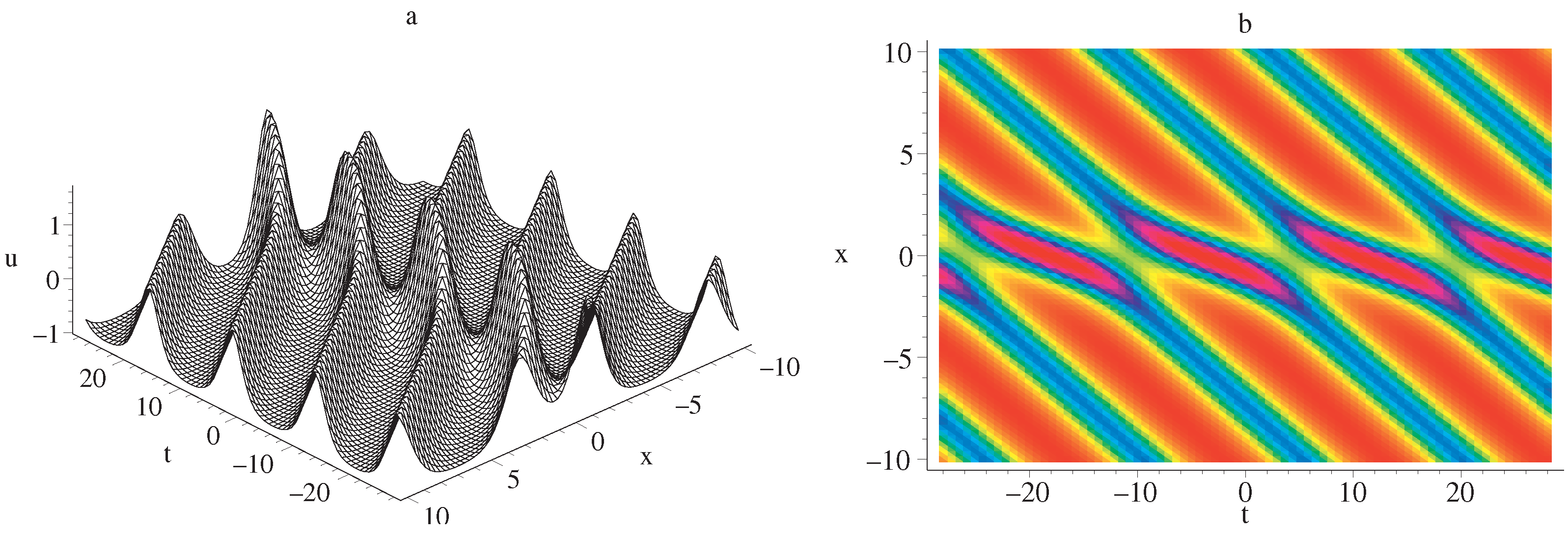
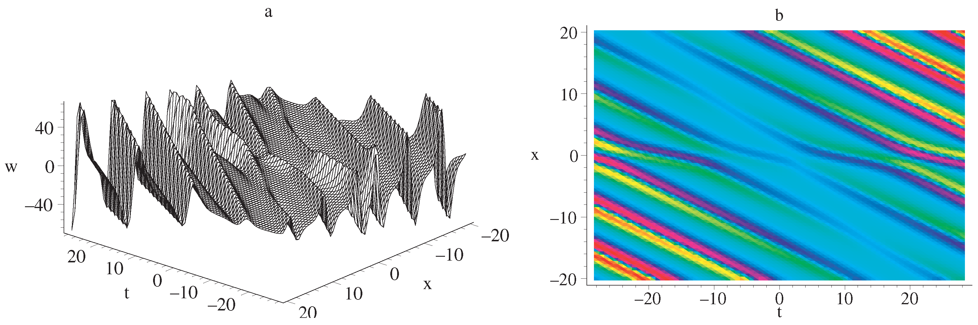
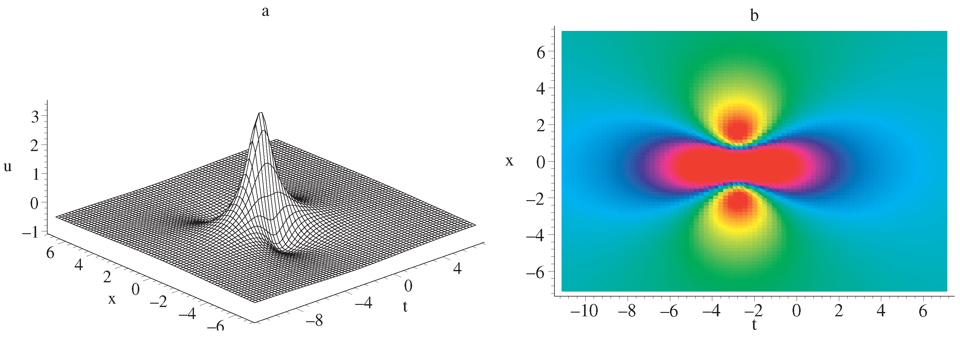
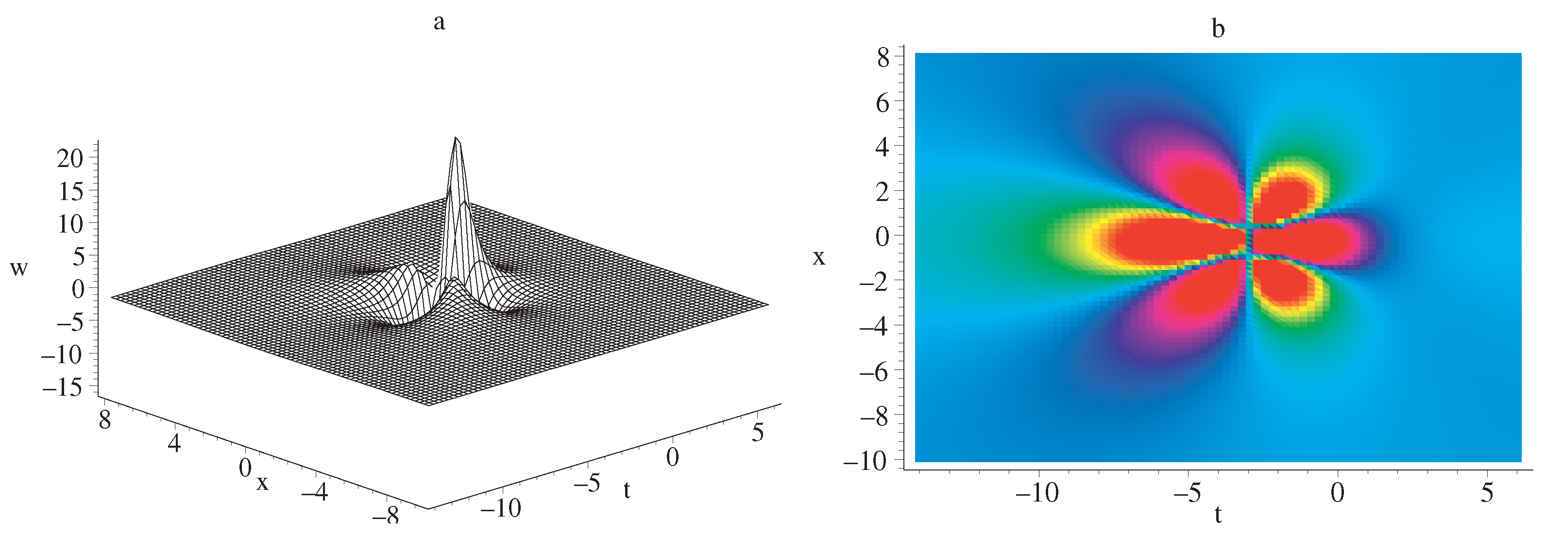
5. Results and Discussion

In this section, we establish a connection between our refinement work and previous results. Based on the mapping and deformation relationship method, the relation between the usual Boussinesq equation and an unknown equation is constructed. Some novel traveling wave solutions are derived by using the mapping and deformation relationship. Additionally, the novel solutions to the BB equation are given through the prior solution and symmetry of the usual Boussinesq equation. By applying the Lie point symmetry, the explicit solutions are given as (21) and (22). By using the multi-soliton (29), the field w of the BB equation is derived as in (31). In the meantime, the interaction between soliton and cnoidal periodic waves is derived by combining a linear solution and a traveling wave. By selecting certain parameters, the interaction between soliton and cnoidal periodic waves of the BB equation are plotted in Figure 1 and Figure 2. The lump wave is given by assuming a quadratic function. The lump wave for the $(1+1)$-dimensional nonlinear system has seldom been studied. By selecting the detail parameters, the lump wave and a special lump wave are plotted in Figure 3 and Figure 4, respectively. Figure 3 and Figure 4 demonstrate that the lump wave rationally localizes in space. The obtained results are novel and have potential applications in supersymmetric systems.

6. Conclusions

Based on the bosonization approach, the Lie point symmetry theory, the mapping and deformation method, the Hirota bilinear method, and the CTE method, some integrability properties and exact solutions for the supersymmetric Boussinesq system are systematically studied. The supersymmetric Boussinesq system is converted into a coupled bosonic system by introducing two additional fermionic parameters. The Lie point symmetry group of the BB equation is determined by using the classical Lie group method. The commutation relations of the infinitesimal generators are consolidated in a table. The group invariant solutions are derived by using symmetry reductions. A specific class of the traveling wave solution of the BB system is generated through the application of the the mapping and deformation method. Some novel solutions can be directly derived from the exact solutions and symmetries of the Boussinesq equation. In the meantime, by combining the Hirota bilinear and CTE approaches, the dynamics of the multi-soliton, soliton–cnoidal interaction solutions, and the lump wave are analyzed in detail. The lump wave has been extensively used in the study of the classical integrable systems. These results are highly meaningful due to the scarcity of such novel solutions in supersymmetric systems. Recently, the Grassmann number and the supersymmetric derivative have been extended to the R-number and the ren-symmetric derivatives. Based on the R-numbers and ren-symmetric derivatives, ren-integrable and ren-symmetric integrable systems have been formulated [35]. Studying the integrability and other complex wave phenomena in supersymmetric and ren-symmetric integrable systems remains a significant problem.

References

1. Hirota, R.; Satsuma, J. Nonlinear evolution equations generated from the Bäklund transformation for the Boussinesq equation. Prog. Theor. Phys. 1977, 57, 797–807. [Google Scholar] [CrossRef]
2. Clarkson, P.A.; Kruskal, M.D. New similarity reductions of the Boussinesq equation. J. Math. Phys. 1989, 30, 2201. [Google Scholar] [CrossRef]
3. Wang, Q.; Mihalache, D.; Beli, M.R.; Zeng, L.W.; Lin, J. Soliton transformation between different potential wells. Opt. Lett. 2023, 48, 747–750. [Google Scholar] [CrossRef]
4. Jia, M.; Lou, S.Y. Searching For (2+1)-dimensional nonlinear Boussinesq equation from (1+1)-dimensional nonlinear Boussinesq equation. Commun. Theor. Phys. 2023, 75, 075006. [Google Scholar] [CrossRef]
5. Tela, G.Y.; Zhang, D.J. On a special coupled lattice system of the discrete Boussinesq type. Rep. Math. Phys. 2023, 91, 219–235. [Google Scholar] [CrossRef]
6. Kupershmidt, B.A. A supe Korteweg-de Vries equation: An integrable system. Phys. Lett. A 1984, 102, 213. [Google Scholar] [CrossRef]
7. Martin, Y.I.; Radul, A.O. A supersymmetric extension of the Kadomtsev-Petviashvili hierarchy. Commun. Math. Phys. 1985, 65, 98. [Google Scholar]
8. Mathieu, P. Supersymmetric extension of the Korteweg-de Vries equation. J. Math. Phys. 1988, 2499, 29. [Google Scholar] [CrossRef]
9. Roelofs, G.H.M.; Kersten, P.H.M. Supersymmetric extensions of the nonlinear Schrödinger equation: Symmetries and coverings. J. Math. Phys. 1992, 2185, 33. [Google Scholar] [CrossRef]
10. Zhang, C.F.; Zhao, Z.L.; Zhang, Y.F. Rational solutions consisting of multiple lump waves and line rogue waves in different spaces of the (3+1)-dimensional Boiti-Leon-Manna-Pempinelli equation in incompressible fluid. Nonlinear Dyn. 2024, 112, 7377–7393. [Google Scholar] [CrossRef]
11. Zhang, X.Q.; Ren, B. Resonance solitons, soliton molecules and hybrid solutions for a (2+1)-dimensional nonlinear wave equation arising in the shallow water wave. Nonlinear Dyn. 2024, 112, 4793–4802. [Google Scholar] [CrossRef]
12. Lou, S.Y.; Hu, X.R.; Chen, Y. Nonlocal symmetries related to Bäcklund transformation and their applications. J Phys. A Math. Theor. 2012, 45, 155209. [Google Scholar] [CrossRef]
13. Ren, B. Symmetry reduction related with nonlocal symmetry for Gardner equation. Commun. Nonlinear Sci. Numer. Simulat. 2017, 42, 456–463. [Google Scholar] [CrossRef]
14. Satsuma, J.; Ablowitz, M.J. Two-dimensional lumps in nonlinear dispersive systems. J. Math. Phys. 1979, 20, 1496–1503. [Google Scholar] [CrossRef]
15. Yang, B.; Yang, J.K. Rogue waves in (2+1)-dimensional three-wave resonant interactions. Phys. D 2022, 432, 133160. [Google Scholar] [CrossRef]
16. Younas, U.; Sulaiman, T.A.; Ren, J.L.; Yusuf, A. Lump interaction phenomena to the nonlinear ill-posed Boussinesq dynamical wave equation. J. Geom. Phys. 2022, 178, 104586. [Google Scholar] [CrossRef]
17. Gao, X.N.; Lou, S.Y.; Tang, X.Y. Bosonization, singularity analysis, nonlocal symmetry reductions and exact solutions of supersymmetric KdV equation. J. High Energy Phys. 2013, 2013, 29. [Google Scholar] [CrossRef]
18. Wei, P.F.; Liu, Y.; Zhan, X.R.; Zhou, J.L.; Ren, B. Bosonization, symmetry reductions, mapping and deformation method for B-extension of Sawada-Kotera equation. Results Phys. 2023, 54, 107132. [Google Scholar] [CrossRef]
19. Das, A.; Huang, W.J.; Roy, S. The supersymmetric Boussinesq equation. Phys. Letts. A 2009, 157, 113. [Google Scholar] [CrossRef]
20. Ren, B.; Lin, J.; Yu, J. Supersymmetric Ito equation: Bosonization and exact solutions. AIP Adv. 2013, 3, 042129. [Google Scholar] [CrossRef]
21. Ren, B. Interaction solutions for supersymmetric mKdV-B equation. Chin. J. Phys. 2015, 53, 56. [Google Scholar] [CrossRef]
22. Ren, B.; Lou, S.Y. A Super mKdV equation: Bosonization, Painlevé property and exact solutions. Commun. Theor. Phys. 2018, 69, 343. [Google Scholar] [CrossRef]
23. Andrea, S.; Restuccia, A.; Sotomayor, A. An operator valued extension of the super Korteweg-de Vries equations. J. Math. Phys. 2001, 42, 2625. [Google Scholar] [CrossRef]
24. Gao, X.N.; Lou, S.Y. Bosonization of supersymmetric KdV equation. Phys. Lett. B 2012, 209, 707. [Google Scholar] [CrossRef]
25. Olver, P.J. Application of Lie Group to Differential Equation; Springer: Berlin, Germany, 1986. [Google Scholar]
26. Tian, S.F.; Xu, M.J.; Zhang, T.T. A symmetry-preserving difference scheme and analytical solutions of a generalized higher-order beam equation. Proc. R. Soc. A 2021, 477, 20210455. [Google Scholar] [CrossRef]
27. Ren, B.; Lin, J.; Wang, W.L. Painlevé analysis, infinite dimensional symmetry group and symmetry reductions for the (2+1)-dimensional Korteweg-de Vries-Sawada-Kotera-Ramani equation. Commun. Theor. Phys. 2023, 75, 085006. [Google Scholar] [CrossRef]
28. Hirota, R. The Direct Method in Soliton Theory; Cambridge University Press: Cambridge, UK, 2004. [Google Scholar]
29. Wazwaz, A.M. Multiple-soliton solutions for the Boussinesq equation. Appl. Math. Comput. 2007, 192, 479–486. [Google Scholar] [CrossRef]
30. Lou, S.Y. Consistent Riccati expansion for integrable systems. Stud. Appl. Math. 2015, 134, 372–402. [Google Scholar] [CrossRef]
31. Ma, W.X. Lump solutions to the Kadomtsev-Petviashvili equation. Phys. Lett. A 2015, 379, 2305. [Google Scholar] [CrossRef]
32. Ren, B.; Ma, W.X.; Yu, J. Characteristics and interactions of solitary and lump waves of a (2+1)-dimensional coupled nonlinear partial differential equation. Nonlinear Dyn. 2019, 96, 717. [Google Scholar] [CrossRef]
33. Ablowitz, M.J.; Satsuma, J. Solitons and rational solutions of nonlinear evolution equations. J. Math. Phys. 1978, 19, 2180. [Google Scholar] [CrossRef]
34. Wei, P.F.; Long, C.X.; Zhu, C.; Zhou, Y.T.; Yu, H.Z.; Ren, B. Soliton molecules, multi-breathers and hybrid solutions in (2+1)-dimensional Korteweg-de Vries-Sawada-Kotera-Ramani equation. Chaos Solitons Fract. 2022, 158, 112062. [Google Scholar] [CrossRef]
35. Lou, S.Y. Ren-integrable and ren-symmetric integrable systems. Commun. Theor. Phys. 2024, 76, 035006. [Google Scholar] [CrossRef]
Figure 1. The interaction between one soliton and cnoidal periodic waves of u is plotted with parameters as (41). (a) The three-dimensional form. (b) The corresponding density form.
Mathematics 12 02002 g001
Figure 2. The interaction between one soliton and cnoidal quasi-periodic waves of w is plotted with parameters as (41). (a) The three-dimensional form. (b) The corresponding density form.
Mathematics 12 02002 g002
Figure 3. The lump wave of u is displayed with parameters as in (45). (a) The three-dimensional form. (b) The corresponding density form.
Mathematics 12 02002 g003
Figure 4. Evolution graph of the special lump wave of w is given by parameters as in (41). (a) The three-dimensional form. (b) The corresponding density form.
Mathematics 12 02002 g004
Disclaimer/Publisher’s Note: The statements, opinions and data contained in all publications are solely those of the individual author(s) and contributor(s) and not of MDPI and/or the editor(s). MDPI and/or the editor(s) disclaim responsibility for any injury to people or property resulting from any ideas, methods, instructions or products referred to in the content.