A Method for Evaluating the Data Integrity of Microseismic Monitoring Systems in Mines Based on a Gradient Boosting Algorithm

Abstract

Microseismic data are widely employed for assessing rockburst risks; however, significant disparities exist in the monitoring capabilities of seismic networks across different mines, and none can capture a complete dataset of microseismic events. Such differences introduce unfairness when applying the same methodologies to evaluate rockburst risks in various mines. This paper proposes a method for assessing the monitoring capability of seismic networks applicable to heterogeneous media in mines. It achieves this by integrating three gradient boosting algorithms: Extreme Gradient Boosting (XGBoost), Light Gradient Boosting Machine (LightGBM), and Categorical Boosting (CatBoost). Initially, the isolation forest algorithm is utilized for preliminary data cleansing, and feature engineering is constructed based on the relative locations of event occurrences to monitoring stations and the working face. Subsequently, the optimal hyperparameters for three models are searched for using 8508 microseismic events from the a Coal Mine in eastern China as samples, and 18 sub-models are trained. Model weights are then determined based on the performance metrics of different algorithms, and an ensemble model is created to predict the monitoring capability of the network. The model demonstrated excellent performance on the training and test sets, achieving log loss, accuracy, and recall scores of 7.13, 0.81, and 0.76 and 6.99, 0.80, and 0.77, respectively. Finally, the method proposed in this study was compared with traditional approaches. The results indicated that, under the same conditions, the proposed method calculated the monitoring capability of the key areas to be 11% lower than that of the traditional methods. The reasons for the differences between these methods were identified and partially explained.

1. Introduction

Rockburst is one of the most serious hazards in underground coal mines. It is described as a sudden and violent dynamic phenomenon of coal and rock mass destruction around mine shafts or working faces due to the instantaneous release of elastic strain energy, often accompanied by phenomena such as coal and rock mass ejection, loud noises, and air blasts [1,2]. In the past few decades, rockbursts have occurred frequently in most mining countries [3,4].

At present, most of the technology used to predict and prevent rockburst disasters utilizes microseismic (MS) monitoring [5,6,7,8]. The data generated can be assessed in various ways to evaluate seismic risk, including trends in MS event frequency and energy [9,10,11], clustering of spatial locations [12], and seismic wave velocity tomography [13,14]. However, due to issues such as the low energy of MS events, limitations in sensor placement, and complex onsite environments, it is challenging to record a complete set of MS data. Therefore, it is necessary to assess the completeness of the monitoring system data before analyzing it and considering its impact [15].

In the field of seismology, there are numerous methods available for assessing the completeness of seismic data. For instance, these methods include statistical seismology methods that assume the magnitude–frequency distribution follows the Gutenberg–Richter (G-R) relation [16], methods based on the magnitude attenuation relationship and noise level to give a theoretical monitoring capability [17], amplitude threshold values [18], and the diurnal signal-to-noise ratio of seismic records [19], as well as methods based on the Probability of Detecting an Earthquake (PDE) approach [20]. Many scholars have used the PDE method to evaluate the earthquake monitoring capability of seismic networks in seven provinces and cities in China, including Shandong, Shanxi, and Liaoning [14,21,22,23,24,25,26].

In the mining field, early studies on the application of the Probability of Detecting an Earthquake (PDE) method in heterogeneous media of mines were conducted by [27,28], among others. Wang and colleagues proposed a workflow for reprocessing seismic data aimed at improving the quality of seismic data to better analyze changes in seismic activity [29,30]. Li and others investigated the evolution characteristics of the detection probability of seismic monitoring systems during the retreat mining period of coal mining faces and further correlated highly integrated seismic data with seismic risk [31].

Gradient boosting machine learning algorithms have seldom been used in the assessment of MS data completeness and seismic network monitoring capability, as indicated by the aforementioned literature. In this work, a novel approach is introduced for evaluating the monitoring capability of seismic networks using three gradient boosting algorithms: Extreme Gradient Boosting (XGBoost), Light Gradient Boosting Machine (LightGBM), and Categorical Boosting (CatBoost). This method is based on 8508 MS events that occurred near a working face of the a Coal Mine in eastern China. Feature engineering is constructed based on the relative locations of event occurrences to monitoring stations and the working face, with the detection of an event by a given monitoring station serving as the label. By inverting the spatial distribution of detection probabilities for MS events by monitoring stations, the network’s detection capability is analyzed.

This approach offers two main advantages over other similar methods. Firstly, it divides the key monitoring area into four sections according to the relative relationship of the area to roadways and working faces, thereby reflecting the impact of heterogeneous mediums. Secondly, it eliminates the need to input the maximum amplitude of each MS event detected by monitoring stations, overcoming a significant obstacle to applying traditional PDE methods in mining scenarios. Traditional PDE methods require the calculation of magnitude differences caused by varying source distances for the same maximum amplitude, which most mine MS catalogs do not record.

The remainder of this paper is organized as follows. Section 2 briefly introduces the theoretical background of the algorithms, including gradient boosting, isolation forest, loss function, and traditional monitoring capability evaluation methods. Section 3 describes the project background, data preprocessing process, and feature engineering details. Section 4 provides a detailed description of the model’s structure, hyperparameters, performance metrics, and the monitoring capabilities of individual stations and the entire monitoring network. Section 5 discusses the impact of feature engineering and oversampling, as well as directions for future improvements. Section 6 summarizes the entire study and presents some conclusions.

2. Theoretical Background

2.1. Gradient Boosting Algorithm

The gradient boosting algorithm is a common and powerful machine learning algorithm that reduces model error by adding weak learners. The most basic gradient boosting algorithm is the Gradient-Boosting Decision Tree (GBDT), which uses decision trees as base learners. It iteratively builds decision trees and uses subsequent trees to correct the errors of previous ones, thus improving the model’s predictive accuracy [32,33,34,35]. During the training process, the residual of the previous decision tree is used as the input for the next tree. Then, by adding new decision trees, the residual is reduced, causing the training loss to decrease in the direction of the negative gradient with each iteration. Ultimately, the prediction result is determined based on the sum of the results of all decision trees.

However, the most utilized gradient boosting algorithms today are not the original GBDT but their enhanced versions. For instance, the XGBoost algorithm was developed by [36] as part of the Distributed Machine Learning Community (DMLC). It has gained widespread acclaim in various machine learning competitions due to its superior predictive performance and is extensively applied in both the academic and industrial sectors. LightGBM, designed by Microsoft Research Asia, employs a histogram-based algorithm to reduce computational overhead and is renowned for its rapid training speed and reduced memory consumption [37]. CatBoost, developed by the Russian company Yandex, can handle categorical features directly without the need for preprocessing. It incorporates the symmetric tree algorithm and the concept of ordered boosting, which helps reduce model overfitting and prediction bias [38].

2.2. Isolation Forest

Isolation forest is an anomaly detection algorithm whose basic principle involves constructing a forest of isolation trees by randomly selecting features and split values. It assumes that samples further away from most data points in the feature space are rarer, thereby isolating them [39,40].

The construction methodology of isolation forests involves the following steps: Initially, a random subset of samples is selected from the dataset. Subsequently, a feature is chosen at random, and a split value is randomly determined between the maximum and minimum values of that feature. The sample subset is then divided into two subsets based on this split value, and these steps are repeated until predefined stopping criteria are met. The determination of whether a sample is an outlier is governed by an anomaly score s, which is calculated based on the sample’s average path length within the trees. The longer the path length of a sample, the higher its probability of being considered an anomaly. The formula for calculating the anomaly score is as follows:

$$s\left(x,n\right)=2^{-\frac{E\left[h\left(x\right)\right]}{c\left(n\right)}}$$

(1)

where $E\left[h\left(x\right)\right]$ is the average path length of data point x across all trees in the forest, n is the number of samples, and $c\left(n\right)$ is the average path length of a data point in a perfectly balanced binary tree. The formula for calculating the $c\left(n\right)$ is

$$c\left(n\right)=2H\left(n-1\right)-\frac{2\left(n-1\right)}{n}$$

(2)

where $H(n-1)$ is harmonic function, which can be approximated as $ln(n-1)+0.5772156649$.

2.3. Loss Function

The logarithmic loss (log loss), commonly utilized in binary classification tasks, serves as a measure to quantify the discrepancy between predicted values and actual outcomes. The objective of learning is to minimize the value of the loss function by adjusting weights. This loss function offers a method to gauge the divergence between the model’s predicted probability distribution and the actual probability distribution, thus assessing the accuracy of the model in inverting the probability space. In binary classification scenarios, the formula for calculating the logarithmic loss is as follows:

$$Loss=-\frac{1}{n}\sum _{i=1}^n\left[y_i\log \left(p_i\right)+\left(1-y_i\right)\log \left(1-p_i\right)\right]-\lambda ·\sum w_i^2$$

(3)

where n is the number of samples, $y_i$ is the actual label of sample $i$, and $p_i$ is the probability predicted by the model that sample $i$ belongs to the positive class, $w$ represents the model’s weight, and $\lambda$ is the parameter for regularization strength.

2.4. Monitoring Capability of Seismic Networks

The core concept for calculating the detection probability of a specific energy MS event at coordinates (x, y, z) by a monitoring network revolves around the combinatorial probabilities of individual stations detecting ($P_D$) or not detecting ($P_N$) the event [20]. Given that the localization of MS events typically necessitates the participation of at least four operational stations, the probability ($P_E$) of an MS event being detected by at least four stations is considered the network’s detection probability for that event. This probability can be calculated by subtracting the probabilities of the event being detected by zero ($P_E^0$), one ($P_E^1$), two ($P_E^1$), and three ($P_E^3$) stations from 1:

$$P_E=1-\sum _{i=0}^3{P}_E^i$$

(4)

The probability of an MS event being detected by 0 stations, $P_E^0$, can be calculated by

$$P_E^0=\prod _{i=1}^s{P}_{N,i}$$

(5)

where s is the number of stations in the network, and $P_{N,i}$ is the probability that station i does not detect the data point.

The probability of a data point being detected by j (≥1) stations, $P_E^j$, can be calculated by

$$P_{\mathrm{E}}^i={\displaystyle \sum _{j=1}^{s{C}_i}}\left[\prod _D{C}_i^s\left(j\right)\prod _N\overline{C_i^s\left(j\right)}\right]$$

(6)

where $s{C}_i$ is the number of combinations of choosing i subsets from s elements, $\prod _D{C}_i^s\left(j\right)$ is the product of the probabilities that the stations selected in the jth permutation and combination can detect the data point, $\prod _N\overline{C_i^s\left(j\right)}$ is the product of the probabilities that the stations not selected in the jth permutation and combination cannot detect the data point.

Combining Equations (4)–(6), the probability $P_E$ that a given data point is detected by at least four stations is as follows:

$$P_E=1-\prod _{i=1}^s{P}_{N,i}-{\displaystyle \sum _{i=0}^3}{\displaystyle \sum _{j=1}^{s{C}_i}}\left[\prod _D{C}_i^s\left(j\right)\prod _N\overline{C_i^s\left(j\right)}\right]$$

(7)

3. Engineering Background and Data Preprocessing

3.1. Project Overview

The energy group that proposed the requirements for this study is one of China’s largest mining conglomerates, with some of its mines at risk of rockburst. Given that MS monitoring is a crucial method for the prevention and observation of rockburst, the group has invested significant resources in this area. However, due to the absence of effective evaluation methods, it is challenging to ascertain the quality of the MS monitoring network construction across different mines. Addressing this issue, this paper presents a method that applies machine learning techniques to evaluate the monitoring capabilities of seismic networks based on data completeness. This method is developed based on 8508 MS events collected between 6 June and 11 September 2023.

During the data collection period, The Coal Mine operated six MS monitoring stations, which were labeled as station_0 to station_5. The planar distribution of these stations is depicted in Figure 1, and their spatial coordinates, along with a brief description, are presented in

Table 1. The information of MS stations.

Station ID	Location	Description
station_0	(20,490,772.166, 3,921,683.424, −658.500)	operational base
station_1	(20,490,811.790, 3,920,503.290, 47.506)	communication building
station_2	(20,489,323.640, 3,920,445.053, −67.741)	silkworm farm
station_3	(20,488,525.520, 3,921,936.055, −144.297)	airshaft
station_4	(20,490,545.540, 3,922,838.660, −657.200)	equipment chamber
station_5	(20,490,811.790, 3,920,503.290, −718.700)	substation

.

In this study, the Python programming language and its associated libraries, such as Pandas and NumPy, were employed for data processing and feature engineering. For the training and evaluation of machine learning models, libraries, including Scikit-learn, XGBoost, LightGBM, and CatBoost, were utilized. To enhance the presentation of results, Matplotlib and Seaborn libraries were used to create various charts and graphs. The development environment mainly comprised Visual Studio Code (VSCode) and Jupyter Notebook.

3.2. Data Preprocessing

Initially, the raw dataset utilized in this paper is derived from the MS monitoring system. It comprises event identifiers (Event ID), the coordinates (x, y, z) where the events occurred, the energy of the events (energy), and the identifiers of the stations (Station ID) used for event localization. A portion of the raw dataset is presented in

Table 2. A portion of the raw dataset.

Event ID	x	y	z	Energy	Station ID
0	20,489,977.04	3,921,589.92	−674.14	576,000	5, 2, 4, 3
1	20,490,097.1	3,920,307.54	−464.18	5490	5, 2, 4, 3
2	20,490,816.49	3,921,648.6	−568.84	3130	5, 2, 4, 3
3	20,489,301.16	3,921,314.16	−906.25	8380	0, 5, 3
4	20,490,259.05	3,921,625.64	−578.04	6007	5, 2, 4
5	20,487,340.09	3,920,151.62	−981.57	12,942	2, 3

.

Subsequently, isolation forests were employed for data cleansing by calculating the anomaly scores for all samples. The data corresponding to the top 10% highest anomaly scores were identified as outliers and were subsequently purged from the dataset. A stratified sampling approach was then adopted to partition the cleansed data, allocating 80% to the training set and 20% to the test set. The distribution of various features within the train and test dataset is illustrated in Figure 2.

In addition, the cleaned dataset was processed to assign unique labels for each monitoring station. A sample in the dataset is labeled ‘1’ if its “Station ID” column contains a specific station; otherwise, it is labeled ‘0’. Figure 3 visualizes the label distribution for each station. In this context, MS events localized using specific stations, denoted by red circles, are represented as cyan scatter points; those not localized by these stations are indicated as grey scatter points. Additionally, the figure employs blue dashed lines to indicate areas of focused monitoring and black dashed lines to highlight regions of the working face pending extraction. This visualization allows for a clear observation of the uneven distribution of MS events and highlights significant variances in the capture capabilities of each monitoring station for these events.

Due to the overlapping of MS events on the plane, it is challenging to intuitively grasp the disparity in the number of MS events across different areas. To address this, Figure 4 presents a statistical analysis of the sample quantity distribution in various subdivisions of the monitoring area. The results indicate a significant imbalance in the spatial distribution of MS events. The majority of events are concentrated in the region extending from 20,489,918 m to 20,490,665 m in the x-direction and from 3,921,145 m to 3,921,846 m in the y-direction, with relatively fewer events in other areas. To mitigate the issue of uneven sample distribution, this study employed an oversampling technique. By replicating samples from sparser areas, their quantity was aligned with that in denser regions. However, in subareas with no samples, no replication was performed.

3.3. Feature Engineering

Effective feature engineering is pivotal to the success of the method. Direct utilization of raw features (x, y, z, energy) for training and prediction can lead to model overfitting, specifically causing an inflated detection probability of MS events at specific locations, which subsequently diminishes the model’s generalization capabilities. In this section, the adopted final approach is introduced, while alternative strategies and their limitations are discussed in the Discussion section.

Initially, the feature set was augmented with the vertical distance (z_distance) and horizontal distance (horizon_distance) between MS events and the stations, enabling the model to learn the patterns of spatial relationships between MS event detection probabilities and station locations.

Subsequently, the key monitoring regions were delineated into four distinct zones—A, B, C, and D—aligned along the straight line connecting the working face and mining roadway, as illustrated in Figure 5. Notably, Area A and Area D correspond to the goaf adjacent to the neighboring working faces, Area B represents the coal seam awaiting extraction, and Area C corresponds to the goaf of the current working face. By identifying whether MS events occur within these specific areas, the heterogeneity of mediums—such as roadways, coal seams, and goaf—was incorporated into the dataset’s features. This approach enables the model to discern the relationship between the detection probability of MS events and the medium in which they are situated.

Lastly, the features representing the MS event locations (x, y, z) were removed from the original dataset, and the logarithm of the energy feature was introduced as an additional feature. The names, data types, and brief descriptions of these features are presented in

Table 3. The information and description of features.

Feature Name	Data Type	Descriptions
z_distance	Float	The vertical distance between the MS event and the station
horizon_distance	Float	The horizontal distance between the MS event and the station
Area A	Boolean	Whether the MS event occurred in Area A
Area B	Boolean	Whether the MS event occurred in Area B
Area C	Boolean	Whether the MS event occurred in Area C
Area D	Boolean	Whether the MS event occurred in Area D
energy	Float	The energy released by the rupture of the MS event source
logenergy	Float	The logarithm of energy

.

4. Results and Analysis

4.1. Structure and Parameters

To enhance the conformity of the model’s fit to the probabilistic space with reality and to mitigate the potential for overfitting of the training set by specific algorithms, an ensemble approach was employed. For each MS monitoring station, individual models were trained using XGBoost, LightGBM, and CatBoost algorithms. Subsequently, weights were assigned to these models based on their training loss (as shown in Section 4.2), culminating in their integration into an ensemble model. This ensemble model encompasses a total of 18 sub-models, with its structure depicted in Figure 6. Moreover, owing to the feature engineering that links the occurrence of MS events to the station locations, each station is equipped with its own train dataset, test dataset, and prediction dataset.

The three algorithmic models employed in this study feature expansive hyperparameter spaces, which necessitate adjustment based on the dataset rather than manual specification. Common hyperparameter optimization techniques include grid search, Bayesian optimization, and random search. Among these, Bayesian optimization employs Bayesian statistical methods to guide the search process. It constructs a probabilistic model of the hyperparameter space and updates this model at each step based on the results of previous evaluations, thereby predicting the parameter combinations most likely to yield the optimal solution. Consequently, Bayesian optimization was utilized to identify the optimal hyperparameters in this research.

In the work, the K-fold cross-validation method was employed for hyperparameter tuning. Each original training set was randomly divided into five subsets of equal size. One subset was used as the validation set, while the remaining four served as the training subsets. This procedure was repeated five times, ensuring that each subset was utilized as the validation set once.

In this study, certain hyperparameters for the XGBoost, LightGBM, and CatBoost algorithms were adjusted, as illustrated in

Table 4. Hyperparameters space and optimal values.

Algorithm	Hyperparameters	Search Range	Stride	Optimal Values
XGBoost	booster	[gbtree, dart]	-	dart
	learning_rate	[0.01, 0.5]	step = 0.01	0.15
	gamma	[1, 10]	step = 0.1	2.6
	max_depth	[3, 10]	step = 1	6
	min_child_weight	[1, 100]	step = 0.01	14.4
	grow_policy	[depthwise, lossguide]	-	depthwise
	max_leaves	[16, 64]	step = 1	41
	subsample	[0.01, 1]	step = 0.01	0.86
	lambda	[1 × 10−10, 100]	log = 10	1.91 × 10−9
	alpha	[1 × 10−10, 100]	log = 10	2.37 × 10−3
	sample_type	[uniform, weighted]	-	uniform
	normalize_type	[tree, forest]	-	forest
	rate_drop	[1 × 10−10, 1]	log = 10	7.68 × 10−2
	skip_drop	[1 × 10−10, 1]	log = 10	2.02 × 10−6
LightGBM	boosting	[gbdt, dart]	-	dart
	learning_rate	[0.01, 0.5]	step = 0.01	0.11
	max_depth	[3, 10]	step = 1	6
	num_leaves	[16, 64]	step = 1	30
	min_data_in_leaf	[20, 200]	step = 2	24
	lambda_l1	[1 × 10−10, 100]	log = 10	7.80 × 10−7
	lambda_l2	[1 × 10−10, 100]	log = 10	2.25 × 10−7
	bagging_fraction	[0.01, 1]	step = 0.01	0.58
	bagging_freq	[1, 10]	step = 1	3
	pos_bagging_fraction	[0.4, 1]	step = 0.01	0.69
	neg_bagging_fraction	[0.4, 1]	step = 0.01	0.69
	drop_rate	[1 × 10−10, 1]	log = 10	1.14 × 10−5
	skip_rate	[1 × 10−10, 1]	log = 10	5.57 × 10−8
CatBoost	learning_rate	[0.01, 0.5]	step = 0.01	0.14
	l2_leaf_reg	[1 × 10−10, 100]	log = 10	27.13
	depth	[3, 10]	step = 1	10
	min_data_in_leaf	[20, 200]	step = 2	26
	colsample_bylevel	[0.01, 1]	step = 0.01	0.84

. For the hyperparameters common across the different algorithmic models, the same search range was designated. Moreover, the maximum average logarithmic loss was employed as the evaluation criterion, and the optimal hyperparameters across all six datasets for each algorithm were synthesized.

The reason for not searching for the number of decision trees (number of iterations) is that, in this study, a larger number of iterations (n_estimators = 500) was set, and pruning and early stopping techniques were used to determine this parameter.

4.2. Performance Metrics

In this study, the primary metric used to evaluate model performance is the log loss, with precision and recall serving as supplementary metrics. The choice of log loss as the principal performance indicator is due to its effectiveness in assessing the model’s accuracy and confidence in predicting the probability space. Additionally, given that the dataset is imbalanced, precision and recall are also adopted as additional metrics to evaluate the model’s performance comprehensively. The performance scores of the 18 sub-models within the ensemble model are detailed in

Table 5. The performance scores of the 18 sub-models within the ensemble model.

Station id	Model	Train			Test
		Log Loss	Precision	Recall	Log Loss	Precision	Recall
0	XGBoost_0	6.46	0.84	0.86	6.40	0.84	0.86
	LightGBM_0	6.43	0.83	0.89	6.13	0.85	0.87
	CatBoost_0	7.24	0.81	0.86	6.60	0.83	0.87
1	XGBoost_1	6.62	0.79	0.13	6.80	0.64	0.12
	LightGBM_1	6.28	0.81	0.16	6.73	0.77	0.12
	CatBoost_1	6.49	0.78	0.13	6.82	0.63	0.12
2	XGBoost_2	4.11	0.89	0.99	4.17	0.88	0.98
	LightGBM_2	4.06	0.89	0.99	4.03	0.89	0.99
	CatBoost_2	4.18	0.88	0.99	4.19	0.88	0.99
3	XGBoost_3	8.81	0.76	0.99	9.09	0.75	0.99
	LightGBM_3	8.84	0.76	0.99	9.03	0.75	0.99
	CatBoost_3	8.94	0.75	0.99	8.83	0.75	0.99
4	XGBoost_4	8.85	0.79	0.74	9.32	0.78	0.71
	LightGBM_4	8.84	0.79	0.75	9.47	0.77	0.74
	CatBoost_4	9.15	0.78	0.73	9.96	0.77	0.70
5	XGBoost_5	7.37	0.80	0.84	5.79	0.86	0.93
	LightGBM_5	7.4	0.80	0.83	5.86	0.86	0.91
	CatBoost_5	8.24	0.77	0.83	6.63	0.84	0.91

.

Within Table 5, certain metrics are reported as 0.99, which indicates a rounding convention distinct from the other values. The specification of a value as 0.99 does not imply rounding down from third decimal places ranging between 0 and 4; rather, it signifies that the actual value exceeds 0.99 but remains less than 1. Additionally, it was found that the six sub-models associated with stations numbered 1 and 4 exhibited notably poorer performance metrics for both training and testing compared to other models. This discrepancy may be attributable to higher local noise levels, longer propagation paths, and the signals’ passage through extensive mined-out regions.

Subsequently, weights were allocated to the ensemble model based on the performance metrics of each algorithm. Given that log loss directly reflects the prediction error of a model, it was prioritized in the weight-allocation strategy. The performance metrics of precision and recall were also considered in this context. Weights were computed using the following formula:

$$W_i=\frac{1}{Loglos{s}_i}\times \left(\frac{Precisio{n}_i+Recal{l}_i}{2}\right)$$

(8)

where $W_i$ is the weight for model i and $Loglos{s}_i$, $Precisio{n}_i$ and $Recal{l}_i$ are the log loss, precision, and recall values for model i. This formula balances the model’s accuracy with its discrimination power for specific classes by multiplying the average of precision and recall with the reciprocal of log loss. Subsequently, the calculated weights $W_i$ for each model were normalized to ensure that the sum of all weights equals 1.

After a statistical analysis of Table 5, it was observed that the mean values for the log loss, precision, and recall metrics for the XGBoost, LightGBM, and CatBoost models are as follows: The XGBoost model exhibited a mean log loss of 6.98, with precision and recall averages of 0.80 and 0.76, respectively. The LightGBM model demonstrated a mean log loss of 7.27, alongside mean precision and recall values of 0.79 and 0.76, respectively. The CatBoost model reported a mean log loss of 6.92, with average precision and recall at 0.81 and 0.77, respectively. Based on these metrics, the final weight allocation for the ensemble model was determined as follows:

$$\mathrm{C}\mathrm{o}\mathrm{m}\mathrm{b}\mathrm{i}\mathrm{n}\mathrm{a}\mathrm{t}\mathrm{i}\mathrm{o}\mathrm{n}=0.336 \ast \mathrm{X}\mathrm{G}\mathrm{B}\mathrm{o}\mathrm{o}\mathrm{s}\mathrm{t}+0.321 \ast \mathrm{L}\mathrm{i}\mathrm{g}\mathrm{h}\mathrm{t}\mathrm{G}\mathrm{B}\mathrm{M}+0.343 \ast \mathrm{C}\mathrm{a}\mathrm{t}\mathrm{B}\mathrm{o}\mathrm{o}\mathrm{s}\mathrm{t}$$

(9)

4.3. Input, Output, and Result

A hypothetical scenario is proposed as the foundation for subsequent analyses in this study: Assume a critical monitoring zone located at an elevation of −650 m, where an MS event of 3000 joules occurs at every 10 m interval along an axis until the entire planar space is occupied. The objective of this scenario is to predict the probability of these MS events. By utilizing the spatial coordinates and energy of the MS events occurring within the hypothetical scenario and following the feature engineering steps outlined in this paper, six input datasets were constructed (as illustrated in Figure 6, labeled input_0 to input_5).

Subsequently, each input dataset was predicted by the respective three models, with the output representing the likelihood of the corresponding station detecting the event (as illustrated in Figure 6, labeled output_0 to output_5). Given the extensive space required to detail the predictive outcomes of all 18 sub-models, along with the results of 6 ensemble models, the predictive outcomes of all sub-models and the ensemble model predictions for stations labeled 0 and 1 are illustrated in Figure 7 and Figure 8, respectively. The predictive outcomes for the ensemble models pertaining to the remaining stations are presented in Figure 9.

From Figure 7, it is apparent that three sub-models captured a significantly lower probability of detection for MS events occurring directly above station_0 compared to other areas. This observation is likely associated with its unique positioning within a substantial underground cavern known as the operational base. Conversely, Figure 8 distinctly demonstrates that station_1 exhibits a uniformly low probability of detecting MS events across the entire key monitoring area, with notably enhanced detection capabilities for events occurring behind the working face compared to those in front. This discrepancy can be attributed to station_1’s location at a surface communication tower, where background noise levels are considerably higher.

Analysis of Figure 9 reveals several intriguing patterns. Notably, there is a generally lower detection probability for MS events occurring in Area C, behind the working face’s goaf. Conversely, MS events occurring in Area D, adjacent to the goaf’s lateral rear, exhibit a higher detection probability. Furthermore, Stations 3 and 4 demonstrate marginally lower detection probabilities for events compared to Stations 2 and 5. This discrepancy underscores a distinct heterogeneity in the detection capabilities across the stations and areas.

Synthesizing the data from Figure 7d, Figure 8d and Figure 9 regarding the detection probability of MS events by various stations under the predefined scenarios in this study, an average detection probability of 0.84 across the monitoring network for these MS events was calculated, with the specific distribution illustrated in Figure 10. In this scenario, the monitoring network’s probability of detecting MS events occurring within Area D is the highest and significantly exceeds that of the other three areas. This observation can also indirectly explain why the number of events detected in Area D slightly surpasses those in other regions. Moreover, the monitoring network exhibits notably lower probabilities of detecting MS events occurring above the operational base (top right corner in the diagram) and behind the mining working face in the goaf areas (bottom left corner in the diagram) compared to other areas.

4.4. Comparison with the Traditional Method

To delineate the distinctions between the novel approach proposed in this paper and conventional methodologies, the traditional PDE method was replicated. Utilizing the same dataset, the detection probabilities of MS events under the predefined scenarios of this study were calculated by the monitoring network, as detailed in Figure 11.

Comparing the PDE method (Figure 10) with the method used in this study (Figure 9), it was found that for microseismic events with an energy of 3000 joules in the key monitoring area, the average detection probability was 0.9 for the PDE method and 0.84 for the method in this study. There are significant differences in the results for the four partitions, ABCD. The method in this study shows detection probabilities of 0.89, 0.87, 0.87, and 0.95 for the four regions, respectively, whereas the traditional PDE method shows detection probabilities of 0.90, 0.92, 0.87, and 0.88. The detection probabilities in regions A and C are very similar for both methods, but the detection probability for region D is significantly higher with the method in this study compared to the PDE method, while the detection probability for region B is significantly higher with the PDE method compared to the method in this study.

In terms of prediction variance, the traditional PDE method demonstrated greater variability, with more pronounced fluctuations in values. Regarding areas of high probability, the traditional PDE method identified the lower half of the key area as having a higher likelihood of event detection, whereas the method indicated the upper left portion of the key area as the high-probability region. In terms of low-probability areas, the traditional PDE method and the research results similarly identified the bottom left and top right portions of the key area as having lower detection probabilities.

The discrepancies between these methods can be attributed to the assumptions underlying the traditional PDE approach, which posits that the medium of propagation is homogeneous and that the detection capability of monitoring stations diminishes with increasing distance and decreasing energy of MS events. Contrarily, the method does not explicitly incorporate these assumptions into the loss function.

5. Discussions

5.1. Influence of Feature Engineering

The impact of feature engineering on machine learning models is substantial and multifaceted, affecting every aspect of model development and performance. Good feature engineering can enhance a model’s accuracy, interpretability, and efficiency in both training and prediction. However, the quantity of features is not a case of the more, the better; instead, it is crucial to ensure the features’ representativeness and their relevance to the problem.

In the initial stages of the experiment, a variety of feature extraction methods were explored. For instance, the distances of MS events from the stations in both the x and y directions were extracted, the clustering labels of MS events and their distances to the cluster centers were calculated using clustering methods, and dimensionality reduction techniques were employed to extract principal components that accounted for 90% of the information contained in all features as supplementary features.

Although these features were somewhat effective in reducing model loss, they significantly compromised the model’s generalization capability. Taking Figure 12 as an example, which depicts the initially predicted detection probability of MS events occurring at an elevation of −650 m with an energy of 500 J by station_5, one can clearly observe many textures perpendicular to the coordinate axes, and the overall image appears cluttered. This phenomenon indicates that the model learned excessively specific patterns and overfitted rules, leading to a decrease in its generalization ability.

5.2. Influence of Oversampling

The dataset utilized in this study predominantly features MS events concentrated within an X coordinate range of 20,489,918 to 20,490,665 m and a Y coordinate range of 3,921,145 to 3,921,846 m, with seismic events in other areas being relatively scarce. Without employing oversampling techniques to balance the sample quantities across various regions, aligning the number of samples in less dense areas with those in denser regions, the model is prone to excessively learning the patterns of samples from the densely populated areas while neglecting the characteristics of samples from other regions. This can lead to a model that overfits the high-density areas and performs poorly when predicting events in areas with fewer historical data points.

5.3. Subsequent Improvements

During the construction of the feature engineering process, the “Area” feature was generated based on the spatial relationship of MS event locations relative to the mining working face and roadways. While these features can, to some extent, reflect the impact of heterogeneous mediums on the monitoring capability of the network, they also introduce clear discontinuities at the boundaries. Incorporating the distance of MS events from the center of their respective areas as a feature in the feature engineering process could potentially mitigate this issue to a certain extent. This approach may provide a smoother transition across area boundaries, thereby reducing abrupt changes in model predictions and enhancing the model’s ability to generalize across different spatial regions.

6. Conclusions

Assessing the completeness of MS data is crucial for enhancing the accuracy of rockburst prediction and prevention. This study introduces a method for evaluating the monitoring capability of seismic networks using three gradient boosting algorithms: XGBoost, LightGBM, and CatBoost. The aim is to analyze MS data completeness to accurately assess the precision of rockburst forecasts and prevention strategies. A case study on the a Coal Mine in eastern China was conducted, utilizing a dataset of 8508 MS data that occurred from 6 June to 11 September 2023. This study reached the following conclusions:

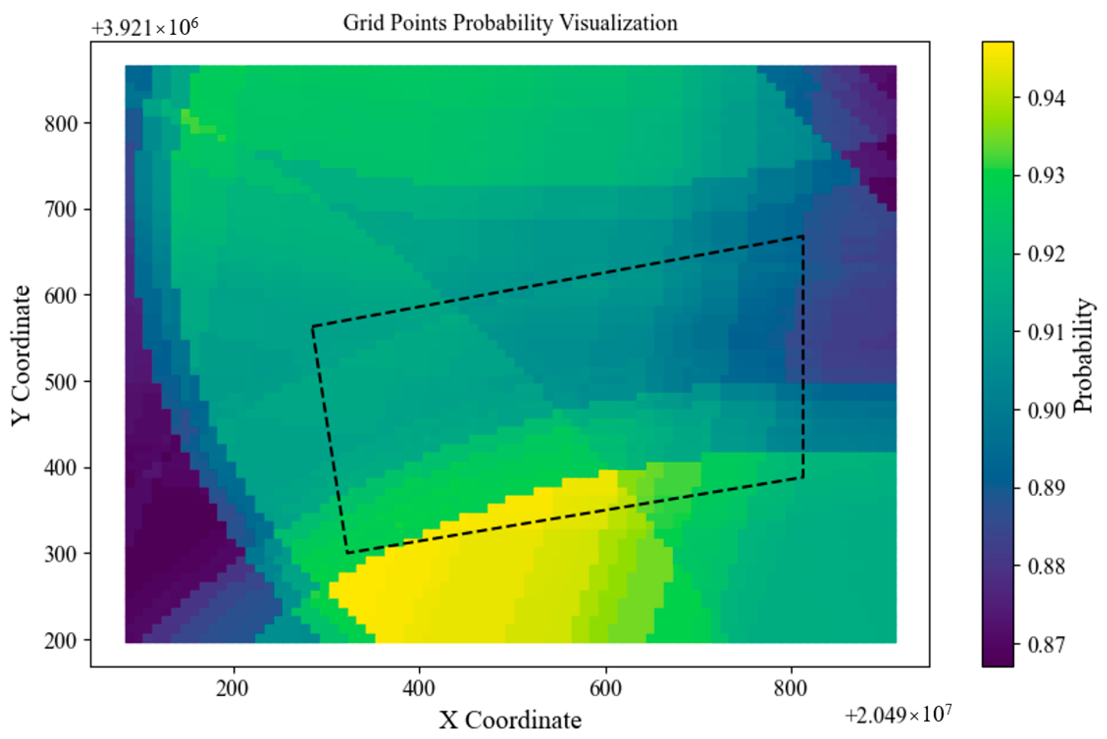
• This method clearly demonstrated the impact of heterogeneous mediums on the monitoring capability of seismic networks. For example, Station 0 exhibited significantly weaker monitoring capability in Areas A and B, Station 1 in Area B, and Station 2 in Area C. Conversely, Station 3 had significantly stronger monitoring capability in Areas B and D, Station 4 in Areas A and D, and Station 5 in Area B;
• The method calculated the detection probability of 3000-joule microseismic events in key monitoring areas to be 0.84, slightly lower than the 0.90 achieved by the traditional PDE method;
• Among the ensemble models, CatBoost performed the best, while LightGBM performed the worst. The ensemble of the three models effectively improved the stability of the results;
• The method overcame two major obstacles in applying the PDE method from earthquake monitoring to mining: the need for extensive nearby searches due to event concentration in specific areas and the necessity of acquiring the maximum amplitude of microseismic events detected by different stations.

References

1. Zhang, C.; Canbulat, I.; Hebblewhite, B.; Ward, C.R. Assessing coal burst phenomena in mining and insights into directions for future research. Int. J. Coal Geol. 2017, 179, 28–44. [Google Scholar] [CrossRef]
2. Cook, N. Seismicity associated with mining. Eng. Geol. 1976, 10, 99–122. [Google Scholar] [CrossRef]
3. Iannacchione, A.T.; Tadolini, S.C. Occurrence, predication, and control of coal burst events in the U.S. Int. J. Min. Sci. Technol. 2016, 26, 39–46. [Google Scholar] [CrossRef]
4. Patyńska, R.; Mirek, A.; Burtan, Z.; Pilecka, E. Rockburst of parameters causing mining disasters in Mines of Upper Silesian Coal Basin. E3S Web Conf. 2018, 36, 03005. [Google Scholar] [CrossRef]
5. Cao, A.-Y.; Dou, L.-M.; Wang, C.-B.; Yao, X.-X.; Dong, J.-Y.; Gu, Y. Microseismic Precursory Characteristics of Rock Burst Hazard in Mining Areas Near a Large Residual Coal Pillar: A Case Study from Xuzhuang Coal Mine, Xuzhou, China. Rock Mech. Rock Eng. 2016, 49, 4407–4422. [Google Scholar] [CrossRef]
6. Srinivasan, C.; Arora, S.; Benady, S. Precursory monitoring of impending rockbursts in Kolar gold mines from microseismic emissions at deeper levels. Int. J. Rock Mech. Min. Sci. Géoméch. Abstr. 1999, 36, 941–948. [Google Scholar] [CrossRef]
7. Wang, G.; Gong, S.; Dou, L.; Wang, H.; Cai, W.; Cao, A. Rockburst characteristics in syncline regions and microseismic precursors based on energy density clouds. Tunn. Undergr. Space Technol. 2018, 81, 83–93. [Google Scholar] [CrossRef]
8. Cai, W.; Dou, L.; Gong, S.; Li, Z.; Yuan, S. Quantitative analysis of seismic velocity tomography in rock burst hazard assessment. Nat. Hazards 2015, 75, 2453–2465. [Google Scholar] [CrossRef]
9. Si, G.; Durucan, S.; Jamnikar, S.; Lazar, J.; Abraham, K.; Korre, A.; Shi, J.-Q.; Zavšek, S.; Mutke, G.; Lurka, A. Seismic monitoring and analysis of excessive gas emissions in heterogeneous coal seams. Int. J. Coal Geol. 2015, 149, 41–54. [Google Scholar] [CrossRef]
10. Cai, W.; Dou, L.; Zhang, M.; Cao, W.; Shi, J.-Q.; Feng, L. A fuzzy comprehensive evaluation methodology for rock burst forecasting using microseismic monitoring. Tunn. Undergr. Space Technol. 2018, 80, 232–245. [Google Scholar] [CrossRef]
11. Cai, W.; Bai, X.X.; Si, G.Y.; Cao, W.Z.; Gong, S.Y.; Dou, L.M. A Monitoring Investigation into Rock Burst Mechanism Based on the Coupled Theory of Static and Dynamic Stresses. Rock Mech. Rock Eng. 2020, 53, 5451–5471. [Google Scholar] [CrossRef]
12. Duan, Y.; Shen, Y.; Canbulat, I.; Luo, X.; Si, G. Classification of clustered microseismic events in a coal mine using machine learning. J. Rock Mech. Geotech. Eng. 2021, 13, 1256–1273. [Google Scholar] [CrossRef]
13. Wang, C.; Cao, A.; Zhu, G.; Jing, G.; Li, J.; Chen, T. Mechanism of rock burst induced by fault slip in an island coal panel and hazard assessment using seismic tomography: A case study from Xuzhuang colliery, Xuzhou, China. Geosci. J. 2017, 21, 469–481. [Google Scholar] [CrossRef]
14. Wang, P.; Bi, B.; Lin, H.; Liu, F.; Shao, Y.; Wang, J. Assessment of Earthquake Monitoring Capability of Shanghai Seismic Network based on PMC Method. Seismol. Geomagn. Obs. Res. 2020, 41, 18–24. (In Chinese) [Google Scholar]
15. Wang, C.; Cao, A.; Zhang, C.; Canbulat, I. A New Method to Assess Coal Burst Risks Using Dynamic and Static Loading Analysis. Rock Mech. Rock Eng. 2020, 53, 1113–1128. [Google Scholar] [CrossRef]
16. Gutenberg, B.; Richter, C.F. Frequency of Earthquakes in California. Bull. Seismol. Soc. Am. 1994, 34, 185–188. [Google Scholar] [CrossRef]
17. Sereno, T.J.; Bratt, S.R. Seismic detection capability at NORESS and implications for the detection threshold of a hypothetical network in the Soviet Union. J. Geophys. Res. 1989, 94, 10397–10414. [Google Scholar] [CrossRef]
18. Gomberg, J. Seismicity and detection/location threshold in the Southern Great Basin Seismic Network. J. Geophys. Res. 1991, 96, 16401–16414. [Google Scholar] [CrossRef]
19. Rydelek, P.A.; Sacks, I.S. Testing the completeness of earthquake catalogues and the hypothesis of self-similarity. Nature 1989, 337, 251–253. [Google Scholar] [CrossRef]
20. Schorlemmer, D.; Woessner, J. Probability of Detecting an Earthquake. Bull. Seism. Soc. Am. 2008, 98, 2103–2117. [Google Scholar] [CrossRef]
21. An, X.; Zhao, Q.; Wang, X.; Wang, S.; Xu, P. Assessment of Earthquake Monitoring Capability of Liaoning Seismic Network Based on PMC Method. China Earthq. Eng. J. 2019, 41, 1545–1552. (In Chinese) [Google Scholar]
22. Peng, L.; Liu, L.; Chen, X.; Zeng, W.; Ding, Y.; Sun, P.; Li, J.; Li, D. Assessment of Earthquake Monitoring Capability of Hainan Seismic Network Based on PMC Method. South China J. Seismol. 2022, 42, 21–28. (In Chinese) [Google Scholar] [CrossRef]
23. Liang, X.; Song, M.; Liu, F.; Liu, L. Assessment of Earthquake Monitoring Capability of Shanxi Seismic Network based on PMC Method. North China Earthq. Sci. 2022, 40, 62–71. (In Chinese) [Google Scholar]
24. Wang, P.; Zheng, J.; Li, B. Analysis of detection capability of Shandong regional seismic network based on PMC method. Prog. Geophys. 2016, 31, 2408–2414. (In Chinese) [Google Scholar]
25. Jiang, C.; Fang, L.; Han, L.; Wang, W.; Guo, L. Assessment of earthquake detection capability for the seismic array: A case study of the Xichang seismic array. Chin. J. Geophys. 2015, 58, 832–843. (In Chinese) [Google Scholar]
26. Guo, Y.; Zhang, L.; Gu, Q.; Huang, H.; Li, Z.; Ma, L. Assessment of Earthquake Monitoring Capability of Qinghai Seismic Network Based on PMC Method. Seismol. Geomagn. Obs. Res. 2022, 43, 23–32. (In Chinese) [Google Scholar]
27. Maghsoudi, S.; Cesca, S.; Hainzl, S.; Kaiser, D.; Becker, D.; Dahm, T. Improving the estimation of detection probability and magnitude of completeness in strongly heterogeneous media, an application to acoustic emission (AE). Geophys. J. Int. 2013, 193, 1556–1569. [Google Scholar] [CrossRef]
28. Plenkers, K.; Schorlemmer, D.; Kwiatek, G.; JAGUARS Research Group. On the Probability of Detecting Picoseismicity. Bull. Seism. Soc. Am. 2011, 101, 2579–2591. [Google Scholar] [CrossRef]
29. Wang, C.; Si, G.; Zhang, C.; Cao, A.; Canbulat, I. A Statistical Method to Assess the Data Integrity and Reliability of Seismic Monitoring Systems in Underground Mines. Rock Mech. Rock Eng. 2021, 54, 5885–5901. [Google Scholar] [CrossRef]
30. Wang, C.; Si, G.; Zhang, C.; Cao, A.; Canbulat, I. Variation of seismicity using reinforced seismic data for coal burst risk assessment in underground mines. Int. J. Rock Mech. Min. Sci. Géoméch. Abstr. 2023, 165, 105363. [Google Scholar] [CrossRef]
31. Li, H.; Cao, A.; Gong, S.; Wang, C.; Zhang, R. Evolution Characteristics of Seismic Detection Probability in Underground Mines and Its Application for Assessing Seismic Risks—A Case Study. Sensors 2022, 22, 3682. [Google Scholar] [CrossRef]
32. Friedman, J.H. Greedy function approximation: A gradient boosting machine. Ann. Stat. 2001, 29, 1189–1232. [Google Scholar] [CrossRef]
33. Bentéjac, C.; Csörgő, A.; Martínez-Muñoz, G. A comparative analysis of gradient boosting algorithms. Artif. Intell. Rev. 2021, 54, 1937–1967. [Google Scholar] [CrossRef]
34. Natekin, A.; Knoll, A. Gradient boosting machines, a tutorial. Front. Neurorobot. 2013, 7, 21. [Google Scholar] [CrossRef]
35. Friedman, J.H. Stochastic gradient boosting. Comput. Stat. Data Anal. 2002, 38, 367–378. [Google Scholar] [CrossRef]
36. Chen, T.; Guestrin, C. XGBoost: A Scalable Tree Boosting System. In Proceedings of the KDD ’16: 22nd ACM SIGKDD International Conference on Knowledge Discovery and Data Mining, San Francisco, CA, USA, 13–17 August 2016; ACM: New York, NY, USA, 2016. [Google Scholar] [CrossRef]
37. Meng, Q. LightGBM: A Highly Efficient Gradient Boosting Decision Tree. In Advances in Neural Information Processing Systems 30, Proceedings of the Annual Conference on Neural Information Processing Systems 2017, Long Beach, CA, USA, 4–9 December 2017; NeurIPS: San Diego, CA, USA, 2017; Volume 30. [Google Scholar]
38. Prokhorenkova, L.; Gusev, G.; Vorobev, A.; Dorogush, A.V.; Gulin, A. CatBoost: Unbiased boosting with categorical features. arXiv 2017. [Google Scholar] [CrossRef]
39. Liu, F.; Ting, K.; Zhou, Z. Isolation Forest. In Proceedings of the IEEE International Conference on Data Mining, Pisa, Italy, 15–19 December 2008. [Google Scholar]
40. Liu, F.T.; Ting, K.M.; Zhou, Z.-H. Isolation-Based Anomaly Detection. ACM Trans. Knowl. Discov. Data 2012, 6, 1–39. [Google Scholar] [CrossRef]
Figure 1. The planar distribution of MS stations.
Mathematics 12 01902 g001
Figure 2. The distribution of various features within train and test dataset.
Mathematics 12 01902 g002
Figure 3. The label distribution for each station. Red dots indicate activated stations, while black dots indicate non-activated stations.
Mathematics 12 01902 g003
Figure 4. The sample quantity distribution in various subdivisions of the monitoring area.
Mathematics 12 01902 g004
Figure 5. Visualization of Areas A, B, C, and D in key monitoring region.
Mathematics 12 01902 g005
Figure 6. The structure of ensemble model.
Mathematics 12 01902 g006
Figure 7. The predictive outcomes of the sub-models and ensemble models for station_0.
Mathematics 12 01902 g007
Figure 8. The predictive outputs of the sub-models and ensemble models for station_1.
Mathematics 12 01902 g008
Figure 9. The predictive outputs of the ensemble models for station_2 to station_5.
Mathematics 12 01902 g009aMathematics 12 01902 g009b
Figure 10. The detection probability of using gradient boosting method.
Mathematics 12 01902 g010
Figure 11. The detection probability of using PDE method.
Mathematics 12 01902 g011
Figure 12. Too many features lead to an imbalance between variance and bias, resulting in poor generalization ability. The red dot represents the station used to calculate the detection probability map for this particular station.
Mathematics 12 01902 g012