Solution of the Elliptic Interface Problem by a Hybrid Mixed Finite Element Method

Abstract

This paper addresses the elliptic interface problem involving jump conditions across the interface. We propose a hybrid mixed finite element method on the triangulation where the interfaces are aligned with the mesh. The second-order elliptic equation is initially decomposed into two equations by introducing a gradient term. Subsequently, weak formulations are applied to these equations. Scheme continuity is enforced using the Lagrange multiplier technique. Finally, we derive an explicit formula for the entries of the matrix equation representing Lagrange multiplier unknowns resulting from hybridization. The method yields approximations of all variables, including the solution and gradient, with optimal order. Furthermore, the matrix representing the final linear algebra systems is not only symmetric but also positive definite. Numerical examples convincingly demonstrate the effectiveness of the hybrid mixed finite element method in addressing elliptic interface problems.

1. Introduction

Many problems are characterized by elliptic equations with discontinuous coefficients in fluid dynamics and solid mechanics, such as variations in density or material composition. For instance, in material mechanics, the challenge of analyzing composite materials with varying densities can be modeled as an elliptic problem with discontinuities. And the propagation of heat conduction processes in different media can result in parabolic problems characterized by discontinuities. The occurrence of jumps in solution and energy flow at interfaces poses intriguing problems in engineering. These problems primarily arise due to the presence of peculiar forces acting on the interface, and further details can be found in [1]. For the numerical solution of the diffusion equation with discontinuous coefficients, the traditional numerical methods include the finite difference method [2,3], finite volume method [4,5], finite element method [6,7,8], and discontinuous finite element method [9,10]. In contrast to problems with continuous coefficients, traditional numerical methods face significant challenges when addressing interface problems with discontinuous coefficients. Methods for solving interface problems encompass the immersion interface method [1], the body-fitted finite element method [8], and the embedding finite element method [9]. Guyomarc employs the local discontinuous finite element method to address the second-order elliptic interface problem [11]. Additionally, Huynh introduces the hybrid intermittent Galerkin (HDG) method in [12]. While the LDG and HDG methods effectively manage complex interfaces and ensure high accuracy, they necessitate the introduction of numerical flux. Careful consideration is essential in selecting stabilization parameters for the numerical flux. In other words, if the chosen parameters are inappropriate, the formulation may become unstable. This paper aims to utilize the hybrid mixed finite element method (HMFE) [13] for solving the two-dimensional elliptic interface problem. In contrast to the LDG and HDG methods, the HMFE method eliminates the need for introducing numerical flux and stabilization parameters. Its format is more concise, and the solution is both more effective and faster. The HMFE method can construct a discrete scheme with high accuracy, and its flexibility in cell division ensures adaptability to complex regions and boundary problems. Choosing the k-order polynomial space as the approximate space for the finite element method ensures that the solution and gradient of the equation achieve (k + 1)-order convergence, which represents the best order under the norm. Given that the matrix of linear equations in HMFE format is symmetric and positive definite, the conjugate gradient method can be effectively employed for solving these equations.

This paper is structured as follows: In Section 2, we provide an introduction to the elliptic interface problem, encompassing discussions on mesh generation and the selection of the approximate space. Section 3 delves into the detailed application of the HMFE method for solving the two-dimensional elliptic interface problem. Finally, we present numerical examples in Section 4 to rigorously validate the efficacy and convergence of the HMFE method in addressing the elliptic interface problem. The paper concludes with a brief summary of the key findings and potential avenues for future research.

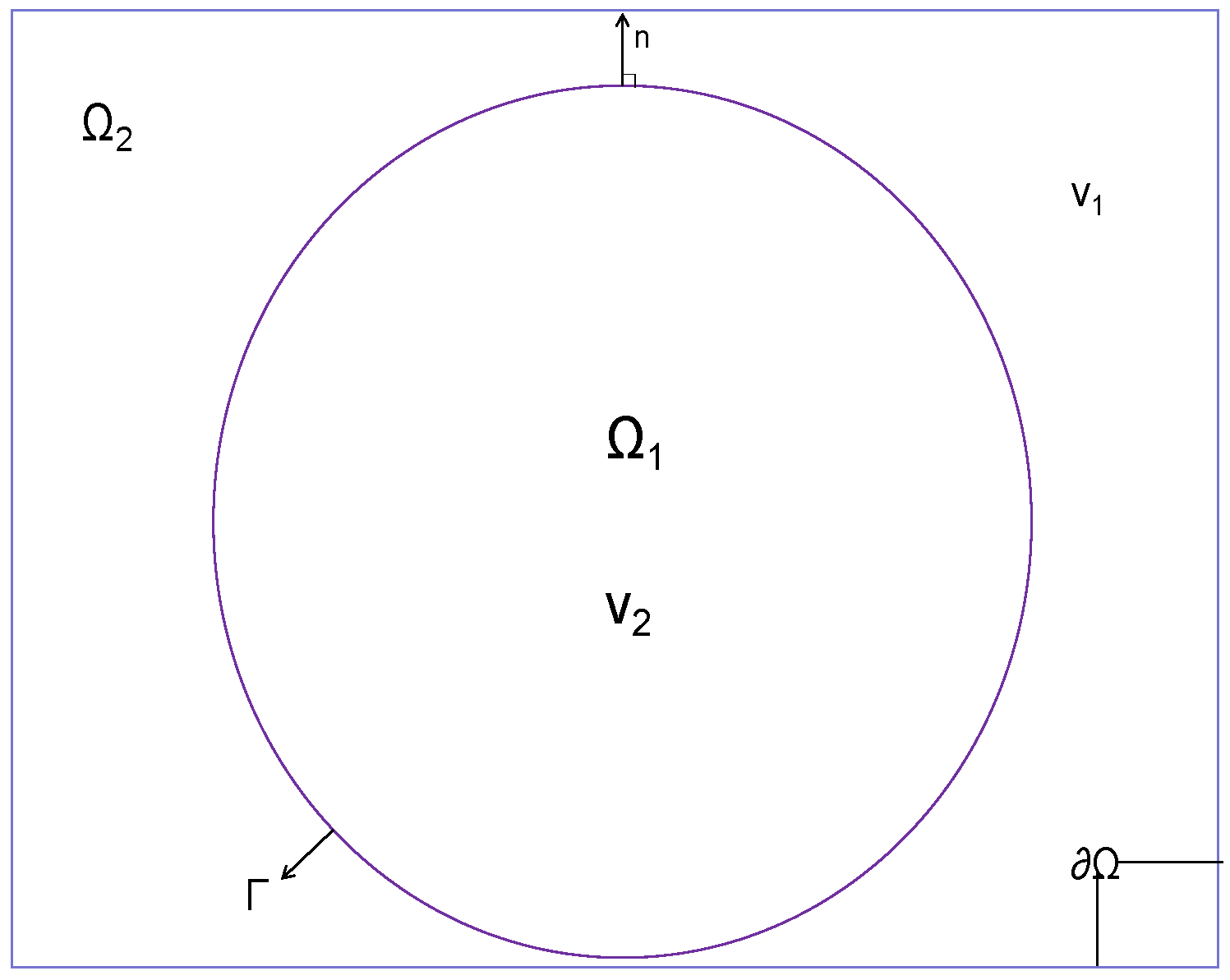
2. Symbolic Description

In this paper, we consider two-dimensional elliptic interface problems:

$$-\nabla ·\left(\kappa (x,y)\nabla u\right)+u=f\left(x,y\right),\left(x,y\right)\in \mathsf{\Omega }$$

(1)

with the boundary conditions

$$u=g_D,\left(x,y\right)\in {\mathsf{\Gamma }}_D,\left(\kappa \left(x,y\right)\nabla u\right)·\mathbf{n}=g_N,\left(x,y\right)\in {\mathsf{\Gamma }}_N$$

(2)

The computational domain is $\mathsf{\Omega }\subset {\mathbf{R}}^2$, and the boundary $\partial \mathsf{\Omega }={\mathsf{\Gamma }}_D\bigcup {\mathsf{\Gamma }}_N$. Assuming that $\mathsf{\Omega }$ contains two sub-domains ${\mathsf{\Omega }}_1,{\mathsf{\Omega }}_2$, which are separated by the interface ${\mathsf{\Gamma }}_I$, we can write $\mathsf{\Omega }$ as $\mathsf{\Omega }={\mathsf{\Omega }}_1\bigcup {\mathsf{\Gamma }}_I\bigcup {\mathsf{\Omega }}_2$, as shown in Figure 1. The multiple sub-domains can be treated similarly. The interface ${\mathsf{\Gamma }}_I$, which belongs to one side of the inner boundary of ${\mathsf{\Omega }}_1,{\mathsf{\Omega }}_2$, can be defined as follows:

$$\begin{array}{c}{\mathsf{\Gamma }}^1=\left\{\mathbf{x}-\epsilon {\mathbf{n}}^1:\mathbf{x}\in \mathsf{\Gamma },\epsilon \to 0\right\},\hfill \\ {\mathsf{\Gamma }}^2=\left\{\mathbf{x}-\epsilon {\mathbf{n}}^2:\mathbf{x}\in \mathsf{\Gamma },\epsilon \to 0\right\},\hfill \end{array}$$

(3)

where ${\mathbf{n}}^1$ is the unit normal vector on the interface ${\mathsf{\Gamma }}_I$ from ${\mathsf{\Omega }}_1$ to ${\mathsf{\Omega }}_2$, and ${\mathbf{n}}^2$ is the unit normal vector on the interface ${\mathsf{\Gamma }}_I$ from ${\mathsf{\Omega }}_2$ to ${\mathsf{\Omega }}_1$. It is assumed that the definition of the diffusion coefficient $\kappa (x,y)$ in the sub-domains ${\mathsf{\Omega }}_1$ and ${\mathsf{\Omega }}_2$ is as follows:

$$\kappa \left(x,y\right)=\left\{\begin{array}{c}{\kappa }_1\left(x,y\right),\left(x,y\right)\in {\mathsf{\Omega }}_1\hfill \\ {\kappa }_2\left(x,y\right),\left(x,y\right)\in {\mathsf{\Omega }}_2\hfill \end{array}\right.$$

(4)

The solution and gradients in the two sub-domains satisfy the following jump conditions at the interface:

$${\left[u\right]}_{{\mathsf{\Gamma }}_I}={\left.u\right|}_{{\mathsf{\Gamma }}^1}-{\left.u\right|}_{{\mathsf{\Gamma }}^2}=s_D$$

(5)

$${\left[-\kappa \nabla u·\mathbf{n}\right]}_{{\mathsf{\Gamma }}_I}=-\left({\kappa }_1{\left.\nabla u\right|}_{{\mathsf{\Gamma }}^1}·{\mathbf{n}}^1+{\kappa }_2{\left.\nabla u\right|}_{{\mathsf{\Gamma }}^2}·{\mathbf{n}}^2\right)=s_N$$

(6)

Here, $s_D$ and $s_N$ are functions defined on the interface that describe the discontinuity in the solution and flux. Physically, this means that there is an abrupt change in the state variable u (such as temperature, electric potential) when crossing the interface from one material to another. Moreover, the rate of flow of the quantity (like heat or charge) is not conserved across the interface, which could represent a source or sink of the quantity at the interface. Now, we use the triangle elements ${\mathcal{T}}_h$ to partition the computational domain $\mathsf{\Omega }$, for which ${\mathcal{T}}_h={\mathcal{T}}_h^1\bigcup {\mathcal{T}}_h^2$, and ${\mathcal{T}}_h^1$ and ${\mathcal{T}}_h^2$ are the sets of the triangle elements K on ${\mathsf{\Omega }}_1$ and ${\mathsf{\Omega }}_2$. The set of boundaries is ${\mathcal{E}}_h^{\partial }={\mathcal{E}}_h^D\bigcup {\mathcal{E}}_h^N$, where ${\mathcal{E}}_h^D$ and ${\mathcal{E}}_h^N$ represent the set of cell boundaries falling on ${\mathsf{\Gamma }}_D$ and ${\mathsf{\Gamma }}_N$, respectively. ${\mathsf{\Gamma }}_h$ is a set of element boundaries falling on the interface and it should be ensured that there is no hanging point at the interface. ${\mathcal{E}}_h^0$ is defined as the set of inner boundaries of all elements, and ${\mathcal{E}}_h$ is defined as the set of all boundary elements boundaries, inner elements boundaries and interface boundaries, that is ${\mathcal{E}}_h={\mathcal{E}}_h^{\partial }\bigcup {\mathcal{E}}_h^0\bigcup {\mathsf{\Gamma }}_h$. Suppose that $e\in {\mathcal{E}}_h$ is a common side of two elements $K_e^{+}$ and $K_e^{-}$, that is, $e=K_e^{+}\bigcap K_e^{-}$. The definition of the trace of the vector function $\mathbf{v}$ on the common side e is as follows: ${\mathbf{v}}_e^{+}=\left\{\mathbf{v}(x,y):(x,y)\in K_e^{+},(x,y)\to e\right\}$, ${\mathbf{v}}_e^{-}=\left\{\mathbf{v}(x,y):(x,y)\in K_e^{-},(x,y)\to e\right\}$.

And the definition of the jump term of the vector function $\mathbf{v}$ on the common side e is $\left[\left[\mathbf{v}\right]\right]={\mathbf{v}}_e^{+}·{\mathbf{n}}_e^{+}+{\mathbf{v}}_e^{-}·{\mathbf{n}}_e^{-}$, where ${\mathbf{n}}_e^{+}$ is a unit normal vector that points from $E_e^{+}$ to $E_e^{-}$ on the boundary e, that is, ${\mathbf{n}}_e^{-}=-{\mathbf{n}}_e^{+}$. If $e\in {\mathcal{E}}_h^{\partial }$, we can have $\left[\left[\mathbf{v}\right]\right]=\mathbf{v}·\mathbf{n}$, where $\mathbf{n}$ is the unit normal vector that points to the outside on the $\mathsf{\Omega }$. Assuming that the interface is assumed to be sufficiently smooth to ensure the normal vector is well defined.

Now, we assume that $P^k\left(D\right)$ denotes the set of all polynomials of degree up to k. Under the definition of element mesh generation, we will introduce the finite element space as:

$$\begin{array}{c}{\mathbf{V}}_h=\left\{\mathbf{v}\in L^2\left({\mathcal{T}}_h\right)\times L^2\left({\mathcal{T}}_h\right):v{|}_K\in P^k\left(K\right)\times P^k\left(K\right)+\mathbf{x}{P}^k\left(K\right),\forall K\in {\mathcal{T}}_h\right\}\\ W_h=\left\{w\in L^2\left({\mathcal{T}}_h\right):w{|}_K\in P^k\left(K\right),\forall K\in {\mathcal{T}}_h\right\}.\end{array}$$

The hybrid finite element is based on the mixed element and introduces the Lagrange multiplier $\lambda$, and the Lagrange multiplier represents the approximate of the trace of u on the boundary $e\in {\mathcal{E}}_h$, which is uniquely defined on each boundary. The introduction of Lagrange multipliers can eliminate the degrees of freedom of the solutions and gradients, and ultimately require solving the equation in which the freedom is $\lambda$. The introduction of the Lagrange multiplier is motivated by the desire to enforce the interface conditions more robustly. The Lagrange multiplier ensures the continuity and compatibility of the solution across the interface. In addition, in order to solve the Lagrange multiplier, we introduce the following space:

$$M_h=\left\{\mu \in L^2\left({\mathcal{E}}_h\right):{\left.\mu \right|}_e\in P^k\left(e\right),\forall e\in {\mathcal{E}}_h\right\}.$$

It is worth noting that basis functions in space $M_h$ are continuous within the element edges, but are discontinuous between boundaries.

3. Hybrid Mixed Finite Element Method

3.1. The Weak Formulation

In this section, we will establish the HMFE scheme for elliptic interface problems (1). By introducing the gradient term $\mathbf{p}=-\kappa (x,y)\nabla u$, Equation (1) can be written as

$$\begin{array}{c}\mathbf{p}=-\kappa \nabla u\hfill \\ u+\nabla ·\mathbf{p}=f\left(x,y\right).\hfill \end{array}$$

(7)

The left- and right-hand sides of the two equations in equation group (7) are multiplied by trial functions $\mathbf{q}$ and v at the same time, and then, we can obtain the following finite element equations by using partial integration:

$$\begin{array}{c}{\int }_K\frac{1}{\kappa }\mathbf{p}·\mathbf{q}dxdy-{\int }_{K}u\nabla ·\mathbf{q}dxdy+{\int }_{\partial K}\tilde{\lambda }\mathbf{q}·\mathbf{n}ds=0\hfill \\ {\int }_K\nabla ·\mathbf{p}vdxdy+{\int }_{K}uvdxdy={\int }_{K}fvdxdy\hfill \end{array}$$

(8)

The aim is to find $\left(\mathbf{p},u\right)\in {\mathbf{V}}_h\times W_h$, for any test functions $\left(\mathbf{q},v\right)\in {\mathbf{V}}_h\times W_h$, so Equation (8) can be established. In order to capture jumps on the interface, the function $\tilde{\lambda }$ here is defined on the basis of the Lagrange multiplier $\lambda$:

$$\tilde{\lambda }=\lambda +{\delta }_{\mathsf{\Gamma }}{S}_D{\delta }_{\mathsf{\Gamma }}=\left\{\begin{array}{cc}1,\hfill & \partial K\bigcap {\mathsf{\Gamma }}_h\ne ⌀\mathrm{and}K\in {\mathcal{T}}_h^1\hfill \\ 0,\hfill & others\hfill \end{array}\right.$$

In order to solve the Lagrange multiplier $\lambda$, we need the third equation, which can weakly impose the continuity condition of the flow on the inner boundary. On the other element boundaries, except the boundary and interface, we need to obtain the flow jump terms of each inner boundary, so that any trial function on it is 0; the flow jump terms can be defined as:

$${\sum }_{e\in {\mathcal{E}}_h^0\setminus {\mathsf{\Gamma }}_h}{\int }_e\mu \left[\left[\mathbf{p}\right]\right]ds=0,\forall \mu \in M_h.$$

By considering Formula (8) on all the elements and considering the boundary conditions and the jumping conditions on the interface, the aim of the hybrid mixed finite element method for the two-dimensional elliptic interface problem is to find $\left(\mathbf{p},u,\lambda \right)\in {\mathbf{V}}_h\times W_h\times M_h$, so that for any test functions $\left(\mathbf{q},v,\mu \right)\in {\mathbf{V}}_h\times W_h\times M_h$, the following can be established:

$$\begin{array}{c}{\int }_{{\mathcal{T}}_h}\frac{1}{\kappa }\mathbf{p}·\mathbf{q}dxdy-{\int }_{{\mathcal{T}}_h}u\nabla ·\mathbf{q}dxdy+{\displaystyle \sum _{e\in {\mathcal{E}}_h^0}}{\int }_e\lambda \left[\left[\mathbf{q}\right]\right]ds=-{\displaystyle \sum _{e\in {\mathcal{E}}_h^D}}{\int }_e{g}_D\left[\left[\mathbf{q}\right]\right]ds-{\displaystyle \sum _{e\in {\mathsf{\Gamma }}_h}}{\int }_e{\delta }_{\mathsf{\Gamma }}{s}_D\mathbf{q}·\mathbf{n}ds\hfill \\ {\int }_{{\mathcal{T}}_h}\nabla ·\mathbf{p}vdxdy+{\int }_{{\mathcal{T}}_h}uvdxdy={\int }_{{\mathcal{T}}_h}fvdxdy\hfill \\ {\displaystyle \sum _{e\in {\mathcal{E}}_h^0\setminus {\mathsf{\Gamma }}_h}}{\int }_e\mu \left[\left[\mathbf{p}\right]\right]ds={\displaystyle \sum _{e\in {\mathsf{\Gamma }}_h}}{\int }_e\mu s_{N}ds+{\displaystyle \sum _{e\in {\mathcal{E}}_h^N}}{\int }_e\mu g_{N}ds\hfill \end{array}$$

(9)

Equation (9) can be transformed into a matrix equation which is not symmetric as:

$$\left(\begin{array}{ccc}\mathbf{A}& -\mathbf{B}& \mathbf{C}\\ {\mathbf{B}}^T& \mathbf{D}& \mathbf{0}\\ {\mathbf{C}}^T& \mathbf{0}& \mathbf{0}\end{array}\right)\left(\begin{array}{c}\mathbf{P}\\ \mathbf{U}\\ \mathsf{\Lambda }\end{array}\right)=\left(\begin{array}{c}\mathbf{g}\\ \mathbf{f}\\ \mathbf{h}\end{array}\right)$$

(10)

where $\mathbf{P},\mathbf{U}$, and $\mathsf{\Lambda }$ are the freedom of $\mathbf{p},u$, and $\lambda$, respectively. And $\mathbf{g}$, $\mathbf{f}$, $\mathbf{h}$ are decided by the right-hand side of (9). From the first equation of equation group (10), we can obtain

$$\mathbf{P}={\mathbf{A}}^{-1}\left(\mathbf{BU}-\mathbf{C}\mathsf{\Lambda }\right)+{\mathbf{A}}^{-1}\mathbf{g}$$

(11)

substituting the above equation into the second equation of equation group (10), we obtain

$${\mathbf{B}}^T{\mathbf{A}}^{-1}\left(\mathbf{BU}-\mathbf{C}\mathsf{\Lambda }\right)+{\mathbf{B}}^T{\mathbf{A}}^{-1}\mathbf{g}+\mathbf{DU}=\mathbf{f}$$

(12)

assuming that $\mathbf{H}={\mathbf{B}}^T{\mathbf{A}}^{-1}\mathbf{B}+\mathbf{D},\begin{array}{c}\end{array}\mathbf{S}={\mathbf{A}}^{-1}\mathbf{B}$, we can have

$$\mathbf{U}=\left({\mathbf{H}}^{-1}{\mathbf{S}}^T\mathbf{C}\right)\mathsf{\Lambda }-{\mathbf{H}}^{-1}{\mathbf{S}}^T\mathbf{g}+{\mathbf{H}}^{-1}\mathbf{f}$$

(13)

substituting $\mathbf{U}$ into (11), and then, substituting in the term ${\mathbf{C}}^T\mathbf{P}=\mathbf{h}$ of the third equations in (10), the following equation can be obtained:

$$\left({\mathbf{C}}^T\mathbf{S}{\mathbf{H}}^{-1}{\mathbf{S}}^T\mathbf{C}-{\mathbf{C}}^T{\mathbf{A}}^{-1}\mathbf{C}\right)\mathsf{\Lambda }-\left({\mathbf{C}}^T\mathbf{S}{\mathbf{H}}^{-1}{\mathbf{S}}^T\right)\mathbf{g}+{\mathbf{C}}^T\mathbf{S}{\mathbf{H}}^{-1}\mathbf{f}+{\mathbf{C}}^T{\mathbf{A}}^{-1}\mathbf{g}=\mathbf{h},$$

(14)

assuming $\mathbf{M}=\mathbf{S}{\mathbf{H}}^{-1}{\mathbf{S}}^T-{\mathbf{A}}^{-1}$, we obtain the equation about $\mathsf{\Lambda }$:

$$\left({\mathbf{C}}^T\mathbf{MC}\right)\mathsf{\Lambda }=\left({\mathbf{C}}^T\mathbf{M}\right)\mathbf{g}-{\mathbf{C}}^T\mathbf{S}{\mathbf{H}}^{-1}\mathbf{f}+\mathbf{h}.$$

(15)

By solving the Lagrange multiplier, the solution of the equation can be obtained. Then, we obtain $\mathbf{U}$ by replacing the solution in (13). Furthermore, the gradient solution $\mathbf{P}$ can be obtained by substituting the solution into (11). It is obvious that the matrix ${\mathbf{C}}^T\mathbf{MC}$ is symmetric and positive definite, so we can apply the conjugate gradient method to solve this system of linear equations [14].

3.2. The Construction of Local Stiffness Matrix

• Case 1. RT0 element

In the lowest-order HMFE formulation for triangular elements, the flux is approximated with vector basis functions that are defined as

$${\mathbf{q}}_{\mathbf{1}}=\left(\begin{array}{c}1\\ 0\end{array}\right),{\mathbf{q}}_{\mathbf{2}}=\left(\begin{array}{c}0\\ 1\end{array}\right),{\mathbf{q}}_{\mathbf{3}}=\left(\begin{array}{c}x-x_T\\ y-y_T\end{array}\right)$$

where $x_T,y_T$ are the center of triangle T. In any point inside element T, $\mathbf{p}$ is approximated by $\mathbf{p}={\displaystyle \sum _{i=1}^3}{p}_i{q}_i$. The local stiffness matrices in (8) are given by $\mathbf{A}=\left|T\right|diag(1,1,\frac{s}{36})$, $\mathbf{B}={\left(0,0,2\left|T\right|\right)}^T,$ where $\left|T\right|$ is its area [15]. Denote by $\partial T=\partial T_1+\partial T_2+\partial T_3$ the three edges of triangle T, which is shown in Figure 2. The corresponding normal vector on the edges of each element is defined as ${\mathbf{n}}_1,{\mathbf{n}}_2,{\mathbf{n}}_3.$ Then, we obtain the local matrix for the Lagrange multiplier as

$$\mathbf{C}=\left[\begin{array}{ccc}{\int }_{\partial T_1}{\mathbf{q}}_1\cdot {\mathbf{n}}_{1}ds& {\int }_{\partial T_2}{\mathbf{q}}_1\cdot {\mathbf{n}}_{2}ds& {\int }_{\partial T_3}{\mathbf{q}}_1\cdot {\mathbf{n}}_{3}ds\\ {\int }_{\partial T_1}{\mathbf{q}}_2\cdot {\mathbf{n}}_{1}ds& {\int }_{\partial T_2}{\mathbf{q}}_2\cdot {\mathbf{n}}_{2}ds& {\int }_{\partial T_3}{\mathbf{q}}_2\cdot {\mathbf{n}}_{3}ds\\ {\int }_{\partial T_1}{\mathbf{q}}_3\cdot {\mathbf{n}}_{1}ds& {\int }_{\partial T_2}{\mathbf{q}}_3\cdot {\mathbf{n}}_{2}ds& {\int }_{\partial T_3}{\mathbf{q}}_3\cdot {\mathbf{n}}_{3}ds\end{array}\right]$$

Here, we use the Gauss formula with three points for the integral on each edge.

• Case 2. RT1 element

In the first-order HMFE formulation for triangular elements, the basis functions for the flux are defined as

$$\begin{array}{c}{\mathbf{q}}_{\mathbf{1}}=\left(\begin{array}{c}1\hfill \\ 0\hfill \end{array}\right),{\mathbf{q}}_{\mathbf{2}}=\left(\begin{array}{c}0\hfill \\ 1\hfill \end{array}\right),{\mathbf{q}}_{\mathbf{3}}=\frac{1}{\sqrt{\left|T\right|}}\left(\begin{array}{c}x-x_T\hfill \\ 0\hfill \end{array}\right),{\mathbf{q}}_{\mathbf{4}}=\frac{1}{\sqrt{\left|T\right|}}\left(\begin{array}{c}0\hfill \\ x-x_T\hfill \end{array}\right),\\ {\mathbf{q}}_{\mathbf{5}}=\frac{1}{\sqrt{\left|T\right|}}\left(\begin{array}{c}y-y_T\hfill \\ 0\hfill \end{array}\right),{\mathbf{q}}_{\mathbf{6}}=\frac{1}{\sqrt{\left|T\right|}}\left(\begin{array}{c}0\hfill \\ y-y_T\hfill \end{array}\right),\\ {\mathbf{q}}_{\mathbf{7}}=\frac{1}{\left|T\right|}\left(\begin{array}{c}{\left(x-x_T\right)}^2\hfill \\ \left(x-x_T\right)\left(y-y_T\right)\hfill \end{array}\right),{\mathbf{q}}_{\mathbf{8}}=\frac{1}{\left|T\right|}\left(\begin{array}{c}\left(x-x_T\right)\left(y-y_T\right)\hfill \\ {\left(y-y_T\right)}^2\hfill \end{array}\right).\end{array}$$

Then, the flux $\mathbf{p}$ is approximated by $\mathbf{p}={\displaystyle \sum _{i=1}^8}{p}_i{q}_i$ in any point inside element T. The local stiffness matrix $\mathbf{A}$ in (8) can be computed by $A={\left[{\int }_T{\mathbf{q}}_i·{\mathbf{q}}_{j}dxdy\right]}_{8\times 8}$. The basis function for u is chosen as

$${\psi }_1=1,{\psi }_2=\frac{1}{\sqrt{\left|T\right|}}\left(x-x_T\right),{\psi }_3=\frac{1}{\sqrt{\left|T\right|}}\left(y-y_T\right).$$

The matrix $\mathbf{B}$ is defined as $\mathbf{B}={\left[{\int }_T\nabla {\psi }_j·{\mathbf{q}}_{i}dxdy\right]}_{8\times 3}.$ Lastly, the basis function for $\tilde{\lambda }$ on each edge is chosen as ${\phi }_1=1,{\phi }_2=\frac{s+1}{2},$ where s is the local coordinate on the edge. And s = 0 on the mid-center of the edge. The corresponding normal vector on the edges of each element is defined as ${\mathbf{n}}_1,{\mathbf{n}}_2,{\mathbf{n}}_3.$ Then, we obtain the local matrix for the Lagrange multiplier as

$$\mathbf{C}=\left[\begin{array}{cccccc}{\int }_{\partial T_1}{\mathbf{q}}_1·{\mathbf{n}}_{1}ds& {\int }_{\partial T_1}\frac{s+1}{2}{\mathbf{q}}_1·{\mathbf{n}}_{1}ds& {\int }_{\partial T_2}{\mathbf{q}}_1·{\mathbf{n}}_{2}ds& {\int }_{\partial T_2}\frac{s+1}{2}{\mathbf{q}}_1·{\mathbf{n}}_{2}ds& {\int }_{\partial T_3}{\mathbf{q}}_1·{\mathbf{n}}_{3}ds& {\int }_{\partial T_3}\frac{s+1}{2}{\mathbf{q}}_1·{\mathbf{n}}_{3}ds\\ {\int }_{\partial T_1}{\mathbf{q}}_2·{\mathbf{n}}_{1}ds& {\int }_{\partial T_1}\frac{s+1}{2}{\mathbf{q}}_2·{\mathbf{n}}_{1}ds& {\int }_{\partial T_2}{\mathbf{q}}_2·{\mathbf{n}}_{2}ds& {\int }_{\partial T_2}\frac{s+1}{2}{\mathbf{q}}_2·{\mathbf{n}}_{2}ds& {\int }_{\partial T_3}{\mathbf{q}}_2·{\mathbf{n}}_{3}ds& {\int }_{\partial T_3}\frac{s+1}{2}{\mathbf{q}}_2·{\mathbf{n}}_{3}ds\\ {\int }_{\partial T_1}{\mathbf{q}}_3·{\mathbf{n}}_{1}ds& {\int }_{\partial T_1}\frac{s+1}{2}{\mathbf{q}}_3·{\mathbf{n}}_{1}ds& {\int }_{\partial T_2}{\mathbf{q}}_3·{\mathbf{n}}_{2}ds& {\int }_{\partial T_2}\frac{s+1}{2}{\mathbf{q}}_3·{\mathbf{n}}_{2}ds& {\int }_{\partial T_3}{\mathbf{q}}_3·{\mathbf{n}}_{3}ds& {\int }_{\partial T_3}\frac{s+1}{2}{\mathbf{q}}_3·{\mathbf{n}}_{3}ds\\ {\int }_{\partial T_1}{\mathbf{q}}_4·{\mathbf{n}}_{1}ds& {\int }_{\partial T_1}\frac{s+1}{2}{\mathbf{q}}_4·{\mathbf{n}}_{1}ds& {\int }_{\partial T_2}{\mathbf{q}}_4·{\mathbf{n}}_{2}ds& {\int }_{\partial T_2}\frac{s+1}{2}{\mathbf{q}}_4·{\mathbf{n}}_{2}ds& {\int }_{\partial T_3}{\mathbf{q}}_4·{\mathbf{n}}_{3}ds& {\int }_{\partial T_3}\frac{s+1}{2}{\mathbf{q}}_4·{\mathbf{n}}_{3}ds\\ {\int }_{\partial T_1}{\mathbf{q}}_5·{\mathbf{n}}_{1}ds& {\int }_{\partial T_1}\frac{s+1}{2}{\mathbf{q}}_5·{\mathbf{n}}_{1}ds& {\int }_{\partial T_2}{\mathbf{q}}_5·{\mathbf{n}}_{2}ds& {\int }_{\partial T_2}\frac{s+1}{2}{\mathbf{q}}_5·{\mathbf{n}}_{2}ds& {\int }_{\partial T_3}{\mathbf{q}}_5·{\mathbf{n}}_{3}ds& {\int }_{\partial T_3}\frac{s+1}{2}{\mathbf{q}}_5·{\mathbf{n}}_{3}ds\\ {\int }_{\partial T_1}{\mathbf{q}}_6·{\mathbf{n}}_{1}ds& {\int }_{\partial T_1}\frac{s+1}{2}{\mathbf{q}}_6·{\mathbf{n}}_{1}ds& {\int }_{\partial T_2}{\mathbf{q}}_6·{\mathbf{n}}_{2}ds& {\int }_{\partial T_2}\frac{s+1}{2}{\mathbf{q}}_6·{\mathbf{n}}_{2}ds& {\int }_{\partial T_3}{\mathbf{q}}_6·{\mathbf{n}}_{3}ds& {\int }_{\partial T_3}\frac{s+1}{2}{\mathbf{q}}_6·{\mathbf{n}}_{3}ds\\ {\int }_{\partial T_1}{\mathbf{q}}_7·{\mathbf{n}}_{1}ds& {\int }_{\partial T_1}\frac{s+1}{2}{\mathbf{q}}_7·{\mathbf{n}}_{1}ds& {\int }_{\partial T_2}{\mathbf{q}}_7·{\mathbf{n}}_{2}ds& {\int }_{\partial T_2}\frac{s+1}{2}{\mathbf{q}}_7·{\mathbf{n}}_{2}ds& {\int }_{\partial T_3}{\mathbf{q}}_7·{\mathbf{n}}_{3}ds& {\int }_{\partial T_3}\frac{s+1}{2}{\mathbf{q}}_7·{\mathbf{n}}_{3}ds\\ {\int }_{\partial T_1}{\mathbf{q}}_8·{\mathbf{n}}_{1}ds& {\int }_{\partial T_1}\frac{s+1}{2}{\mathbf{q}}_8·{\mathbf{n}}_{1}ds& {\int }_{\partial T_2}{\mathbf{q}}_8·{\mathbf{n}}_{2}ds& {\int }_{\partial T_2}\frac{s+1}{2}{\mathbf{q}}_8·{\mathbf{n}}_{2}ds& {\int }_{\partial T_3}{\mathbf{q}}_8·{\mathbf{n}}_{3}ds& {\int }_{\partial T_3}\frac{s+1}{2}{\mathbf{q}}_8·{\mathbf{n}}_{3}ds\end{array}\right]$$

Here, we use the Gauss formula with three points for the integral on each edge.

4. Numerical Examples

In this section, we use the hybrid mixed finite element method to solve the interface problem. Two numerical examples are given. The first numerical example is the case of a discontinuous coefficient, but the solution and the flow are continuous at the interface; the second example is the interface problem, and the solution and the flow both jump at the interface. In this paper, the numerical example is programmed by Matlab 2016a.

• Example 1. (Discontinuous coefficient problem)

Considering the two-dimensional discontinuous coefficient problem (1), the computational domain is $\mathsf{\Omega }={\left[0,1\right]}^2$, select the interface as a circle centered on point $\left(0.5,0.5\right)$ and radius $R=0.25$, $\mathsf{\Gamma }=\left\{\left(x,y\right)\left|{\left(x-0.5\right)}^2+{\left(y-0.5\right)}^2=R^2\right.\right\}.$ The diffusion coefficient is chosen as

$$\kappa \left(x,y\right)=\left\{\begin{array}{c}{d}_1,\begin{array}{c}\end{array}r\le R\hfill \\ d_2,\begin{array}{c}\end{array}r>R\hfill \end{array}\right.$$

The solution and gradient on the interface satisfy the following jump conditions: ${\left[u\right]}_{\mathsf{\Gamma }}=0$,

$${\left[-\kappa \nabla u·\mathbf{n}\right]}_{\mathsf{\Gamma }}=0.$$

The problem has the exact solution

$$u=\left\{\begin{array}{c}\frac{r^3}{d_1},\begin{array}{c}\end{array}\begin{array}{cccc}\begin{array}{cc}& \end{array}& & & \end{array}r\le R\hfill \\ \frac{r^3}{d_2}+\left(\frac{1}{d_1}-\frac{1}{d_2}\right)R^3,\begin{array}{c}\end{array}r>R\hfill \end{array}\right.$$

where $r=\sqrt{{\left(x-0.5\right)}^2+{\left(y-0.5\right)}^2}$. We use three different meshes: the number of elements are $N{e}_1=2418,\begin{array}{c}\end{array}N{e}_2=9556,\begin{array}{c}\end{array}N{e}_3=37,952$. We solve this problem using the RT0 and RT1 elements.

The errors based on the $L_2$ norm are shown in

Table 1. The convergence analysis of example 1 for RT0.

Diffusion Coefficient	Number of Elements	${∥\mathit{u}-{\mathit{u}}_{\mathit{h}}∥}_{{\mathit{L}}_2}$	Convergence Order	${∥\mathbf{p}-{\mathbf{p}}_{\mathit{h}}∥}_{{\mathit{L}}_2}$	Convergence Order
$d_1={10}^{-2},d_2=1$	2418	3.01 × 10${ }^{-2}$	-	1.68 × 10${ }^{-2}$	-
$d_1={10}^{-2},d_2=1$	9556	1.53 × 10${ }^{-2}$	0.98	4.16 × 10${ }^{-3}$	1.01
$d_1={10}^{-2},d_2=1$	37,952	7.72 × 10${ }^{-3}$	0.99	1.10 × 10${ }^{-3}$	1.00

and

Table 2. The convergence analysis of example 1 for RT1.

Diffusion Coefficient	Number of Elements	${∥\mathit{u}-{\mathit{u}}_{\mathit{h}}∥}_{{\mathit{L}}_2}$	Convergence Order	${∥\mathbf{p}-{\mathbf{p}}_{\mathit{h}}∥}_{{\mathit{L}}_2}$	Convergence Order
$d_1={10}^{-2},d_2=1$	2418	2.82 × 10${ }^{-3}$	-	7.83 × 10${ }^{-3}$	-
$d_1={10}^{-2},d_2=1$	9556	7.05 × 10${ }^{-4}$	1.99	2.76 × 10${ }^{-3}$	1.54
$d_1={10}^{-2},d_2=1$	37,952	1.76 × 10${ }^{-4}$	1.99	9.72 × 10${ }^{-4}$	1.52

. The results show that the convergence order of solution u can reach the accuracy of first order and second order with the $R{T}_0$ and $R{T}_1$ elements, respectively. We also observe an experimental convergence order of 1 and 1.5 for the gradient term with the $R{T}_0$ and $R{T}_1$ elements, respectively. The numerical solution is shown in Figure 3. The results show that the HMFE method can accurately capture the discontinuous area of the derivative.

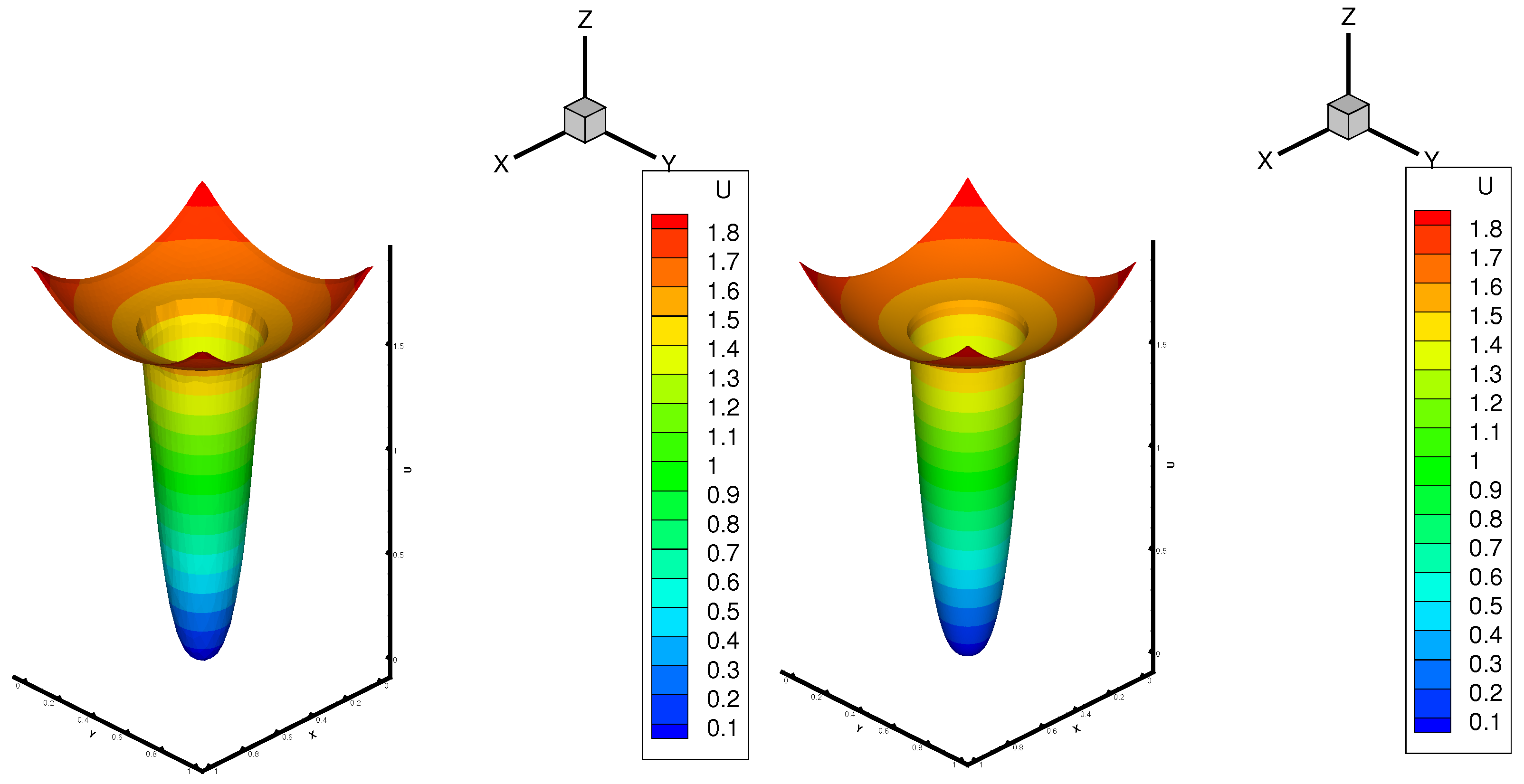
• Example 2. (Interface Problem).

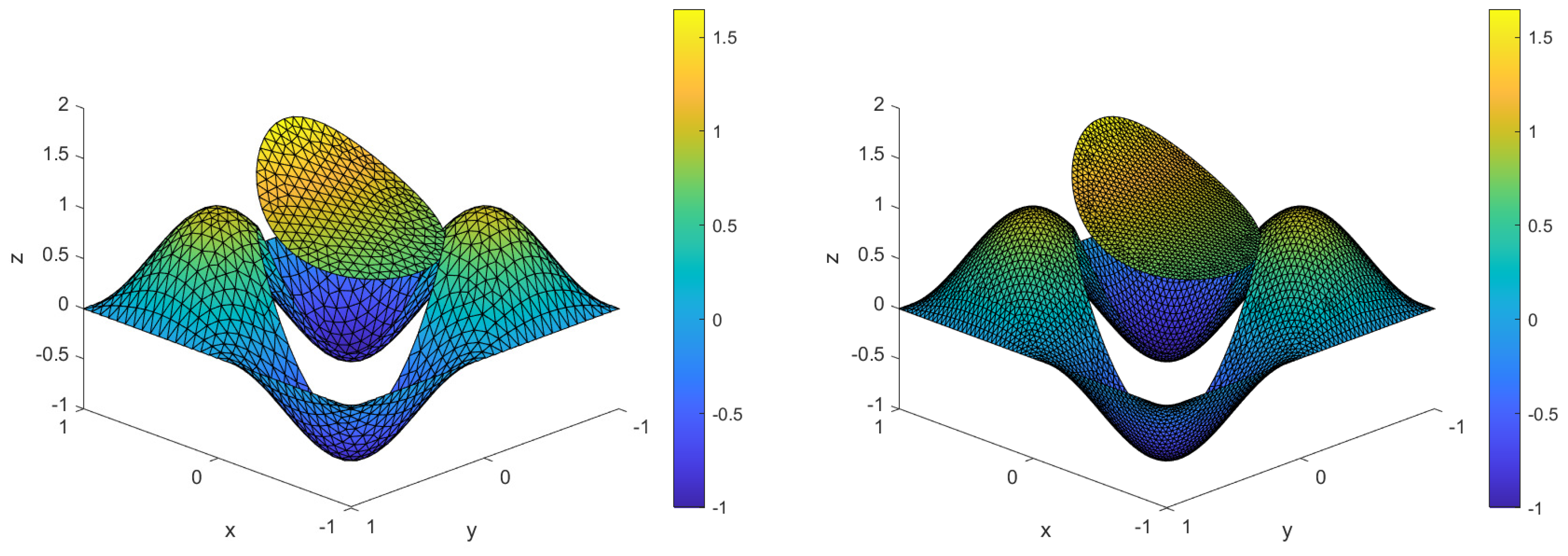
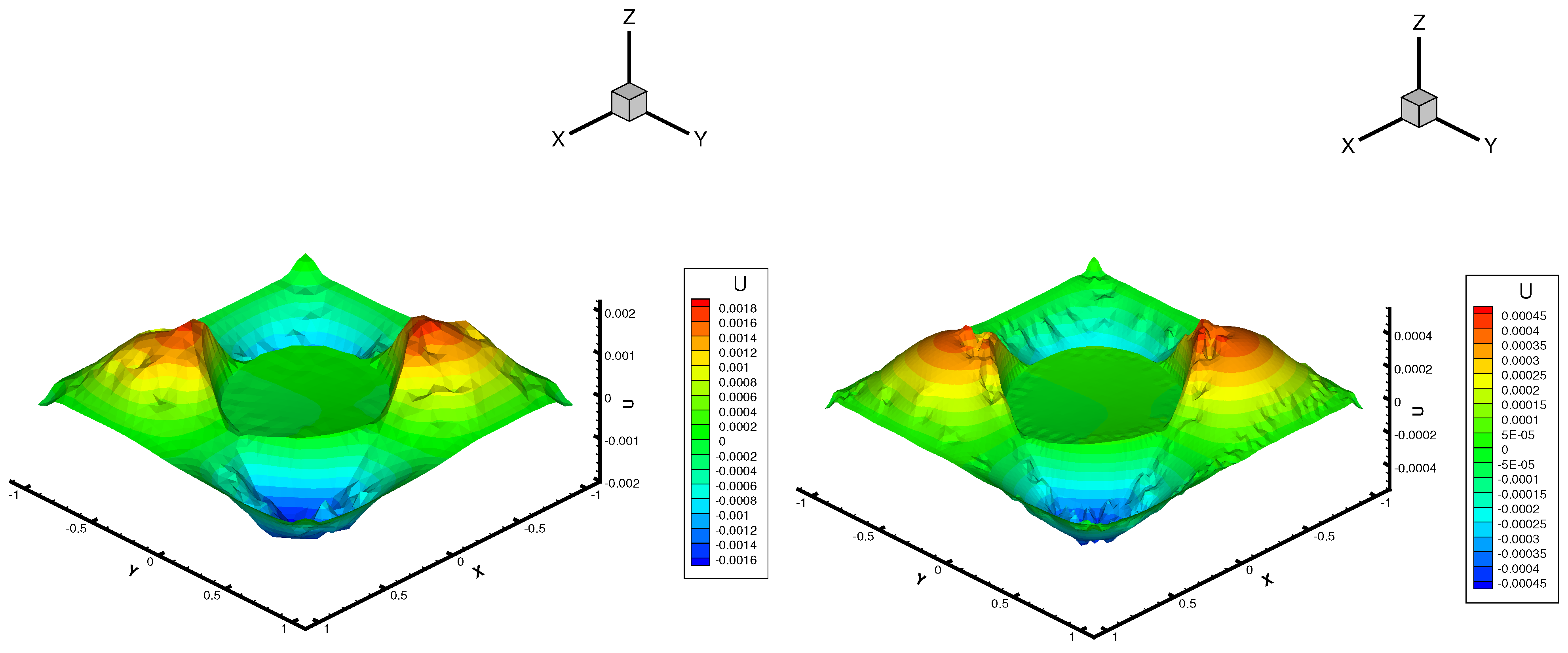
Consider the elliptic problems (1) with discontinuous coefficients. The computational domain is $\mathsf{\Omega }={\left[-1,1\right]}^2$, the interface is $\mathsf{\Gamma }=\left\{\left(x,y\right)\left|x^2+y^2={0.5}^2\right.\right\}$, and ${\mathsf{\Omega }}_1=\left\{\left(x,y\right)\left|x^2+y^2\le {0.5}^2\right.\right\},$$\begin{array}{c}\end{array}{\mathsf{\Omega }}_2=\mathsf{\Omega }\setminus {\mathsf{\Omega }}_1$, and the diffusion coefficient of this problem is $\kappa \left(x,y\right)\equiv 1$. The solution and flow at the interface satisfy the following jump conditions:

$${\left[u\right]}_{{\mathsf{\Gamma }}_I}={\mathrm{e}}^x\cos \left(\mathrm{y}\right)-\sin (\pi \mathrm{x}\left)\sin \right(\pi \mathrm{y});$$

$${\left[-\kappa \nabla u·\mathbf{n}\right]}_{{\mathsf{\Gamma }}_I}=2\mathrm{x}\left(\pi \cos (\pi \mathrm{x}\left)\sin \right(\pi \mathrm{y})-{\mathrm{e}}^x\cos \left(\mathrm{y}\right)\right)+2\mathrm{y}\left(\pi \sin (\pi \mathrm{x}\left)\cos \right(\pi \mathrm{y})+{\mathrm{e}}^x\sin \left(\mathrm{y}\right)\right)$$

The exact solution of this problem is

$$u=\left\{\begin{array}{c}{\mathrm{e}}^x\cos \left(\mathrm{y}\right),\begin{array}{ccc}& & \left(x,y\right)\in {\mathsf{\Omega }}_1\end{array}\hfill \\ \sin (\pi \mathrm{x}\left)\sin \right(\pi \mathrm{y}),\begin{array}{c}\end{array}\left(x,y\right)\in {\mathsf{\Omega }}_2\hfill \end{array}\right.$$

The $L_2$ errors of the solution u and flow p are shown in

Table 3. Convergence analysis of example 2 for RT0.

Number of Elements	${∥\mathit{u}-{\mathit{u}}_{\mathit{h}}∥}_{{\mathit{L}}_2}$	Convergence Order	${∥\mathbf{p}-{\mathbf{p}}_{\mathit{h}}∥}_{{\mathit{L}}_2}$	Convergence Order
2418	5.21 × 10${ }^{-2}$	-	2.19 × 10${ }^{-1}$	-
9556	2.60 × 10${ }^{-2}$	1.00	1.10 × 10${ }^{-1}$	1.00
37,952	1.30 × 10${ }^{-2}$	1.00	5.49 × 10${ }^{-2}$	1.00

and

Table 4. Convergence analysis of example 2 for RT1.

Number of Elements	${∥\mathit{u}-{\mathit{u}}_{\mathit{h}}∥}_{{\mathit{L}}_2}$	Convergence Order	${∥\mathbf{p}-{\mathbf{p}}_{\mathit{h}}∥}_{{\mathit{L}}_2}$	Convergence Order
2418	1.62 × 10${ }^{-3}$	-	1.48 × 10${ }^{-2}$	-
9556	3.88 × 10${ }^{-4}$	2.06	5.08 × 10${ }^{-3}$	1.54
37,952	9.64 × 10${ }^{-5}$	2.00	1.77 × 10${ }^{-3}$	1.52

, respectively. We observe similar convergence orders. The numerical solutions at t = 1 are shown in Figure 4, in which the left one contains 2418 triangles and the right one contains 9556 triangles. Figure 5 shows the contours of the errors with two triangulations.

• Example 3.

In paraxial approximations for wave propagations in optical waveguides, Schrödinger equations are applied to solve the propagation direction. Due to the mismatch of refractive indices in waveguides, the electromagnetic fields are discontinuous solutions to Schrödinger equations. It is simple to extend these principles to a broader class of problems by incorporating time. In this example, the time is discretized and the spatial components and interface conditions still align with the elliptic interface problem’s methodology; the following two-dimensional Schrödinger equation is employed to demonstrate the discontinuous wave propagation:

$$ic\frac{\partial \phi }{\partial t}={\nabla }^2\phi (x,y,t)$$

The jump conditions for Equations (5) and (6) are given in the following:

$$\begin{array}{c}{\left[u\right]}_{{\mathsf{\Gamma }}_I}=e^{i{E}_{2}t}{e}^{i{k}_{x2}x+i{k}_{y2}y}-e^{i{E}_{1}t}{e}^{i{k}_{x1}x+i{k}_{y1}y}\\ {\left[-\kappa \nabla u·\mathbf{n}\right]}_{{\mathsf{\Gamma }}_I}=e^{i{E}_{2}t}(i{k}_{x_2}x+i{k}_{y_2}y)e^{i{k}_{x2}x+i{k}_{y2}y}-e^{i{E}_{1}t}(i{k}_{x_1}x+i{k}_{y_1}y)e^{i{k}_{x1}x+i{k}_{y1}y}\end{array}$$

where $E_i=\left(k_{x_i}^2+k_{y_i}^2\right)/c_i$ for $i=1,2$ and ${\mathsf{\Omega }}_1=\left\{\left(x,y\right)|x^2+y^2\le 1\right\},{\mathsf{\Omega }}_2=\left\{\left(x,y\right)|1\le x^2+y^2\le 2\right\}.$ Then, the time term is discretized as

$$ic\frac{{\phi }_{n+1}-{\phi }_n}{\Delta t}={\nabla }^2{\phi }_{n+1}\left(x,y,t\right),$$

setting $\mathbf{q}=-\nabla {\phi }_{n+1}$, we obtain

$$ic\frac{{\phi }_{n+1}}{\Delta t}+\nabla ·\mathbf{q}=ic\frac{{\phi }_n}{\Delta t}.$$

The parameters are chosen as $k_{x1}=k_{x2}=k_{x3}=2,k_{y1}=3,c_1=3,c_2=3.1,A_1=A_2=1$, $B_1=B_2=0$, and the jump is given at the interface. Starting from t = 0, the solution is computed up to t = 1 with a time step $\Delta t=1d-4$. Figure 6 shows the real and imaginary parts of the numerical results using the HMFE method with three different meshes.

5. Conclusions

(1)

The matrix of the linear system of equations in the HMFE format is symmetric positive definite, thus enabling the application of the conjugate gradient method to solve the system of equations. Compared to LDG and HDG methods, the HMFE method does not require the introduction of numerical fluxes and stabilization parameters, making its formulation more concise. Through comprehensive numerical examples, the effectiveness and convergence of the HMFE method are validated.

(2)

The proposed hybrid mixed finite element (HMFE) method achieves second-order accuracy and the convergence orders for the gradient term are order 1 and 1.5 with RT0 and RT1 elements, providing significant improvements over first-order methods. Detailed error analysis shows optimal order convergence for both the solution and its gradient, crucial for applications needing precise gradient computations.

(3)

Low-order terms $+u$ and jump conditions are introduced. The inclusion of low-order terms and the enforcement of jump conditions play a critical role in accurately capturing the physical behavior at interfaces. These elements ensure the solution and its flux meet the necessary discontinuities, effectively representing phenomena like sources or sinks and enhancing the method’s overall accuracy and applicability in complex interface problems.

Future Work: While the current work focused on two-dimensional problems, future research will extend the HMFE method to three-dimensional interface problems. Additionally, further studies will explore adaptive mesh refinement techniques to enhance the computational efficiency and accuracy of the method in handling more complex geometries and boundary conditions.

References

1. Leveque, R.J.; Li, Z. The immersed interface method for elliptic equations with discontinuous coefficients and singular sources. Siam J. Numer. Anal. 1994, 31, 1019–1044. [Google Scholar] [CrossRef]
2. Qin, Q.; Song, L.; Wang, Q. High-order meshless method based on the generalized finite difference method for 2D and 3D elliptic interface problems. Appl. Math. Lett. 2023, 137, 108479. [Google Scholar] [CrossRef]
3. Li, D.Y.; Dong, S.Q. Segment explicit-implicit schemes for a parabolic equation with discontinuous coefficients. Math. Numer. Sin. 1997, 19, 193–204. [Google Scholar]
4. Wang, Q.; Zhang, Z.; Wang, L. New immersed finite volume element method for elliptic interface problems with non-homogeneous jump conditions. J. Comput. Phys. 2021, 427, 110075. [Google Scholar] [CrossRef]
5. Vieira, L.M.; Giacomini, M.; Sevilla, R.; Huerta, A. A second-order face-centred finite volume method for elliptic problems. Comput. Methods Appl. Mech. Eng. 2020, 358, 112655. [Google Scholar] [CrossRef]
6. Chen, Y.; Li, Q.; Wang, Y.; Huang, Y. Two-grid methods of finite element solutions for semi-linear elliptic interface problems. Numer. Algorithms 2020, 84, 307–330. [Google Scholar] [CrossRef]
7. Guo, R.; Lin, T. An immersed finite element method for elliptic interface problems in three dimensions. J. Comput. Phys. 2020, 414, 109478. [Google Scholar] [CrossRef]
8. Lin, T.; Sheen, D.; Zhang, X. A nonconforming immersed finite element method for elliptic interface problems. J. Sci. Comput. 2019, 79, 442–463. [Google Scholar] [CrossRef]
9. Zhuang, Q.; Guo, R. High degree discontinuous Petrov–Galerkin immersed finite element methods using fictitious elements for elliptic interface problems. J. Comput. Appl. Math. 2019, 362, 560–573. [Google Scholar] [CrossRef]
10. Zhu, J.; Poblete, H.A.V. Robust And Efficient Mixed Hybrid Discontinuous Finite Element Methods for Elliptic Interface Problems. Int. J. Numer. Anal. Model. 2019, 16, 767–788. [Google Scholar]
11. Guyomarc’h, G.; Lee, C.O.; Jeon, K. A discontinuous Galerkin methods for elliptic interface problems with application to electroporation. Commun. Numer. Methods Eng. 2009, 25, 991–1008. [Google Scholar] [CrossRef]
12. Huynh, L.N.T.; Nguyen, N.C.; Peraire, J.; Khoo, B.C. A high-order hybridizable discontinuous Galerkin method for elliptic interface problems. Int. J. Numer. Meth. Eng. 2013, 93, 183–200. [Google Scholar] [CrossRef]
13. Cockburn, B.; Gopalakrishnan, J. A chracterization of hybridized mixed methods for second order elliptic problems. SIAM J. Numer. Anal. 2005, 42, 283–301. [Google Scholar] [CrossRef]
14. Boffi, D.; Brezzi, F.; Fortin, M. Mixed Finite Element Methods and Applications; Springer: Heidelberg/Berlin, Germany, 2013. [Google Scholar]
15. Bahriawati, C.; Carstensen, C. Three MATLAB implementations of the lowest-order Raviart-Thomas MFEM with a posteriori error control. Comput. Methods Appl. Math. 2005, 5, 333–361. [Google Scholar] [CrossRef]
Figure 1. The computation domain separated by the interface.
Mathematics 12 01892 g001
Figure 2. Triangle T with vertices and opposite edges T 1 , T 2 , and T 3 .
Mathematics 12 01892 g002
Figure 3. Numerical results of example 1.
Mathematics 12 01892 g003
Figure 4. The numerical solution of example 2.
Mathematics 12 01892 g004
Figure 5. The contours of errors with three triangulations.
Mathematics 12 01892 g005
Figure 6. The real and imaginary numerical solutions of example 3 at t = 1 with different meshes.
Mathematics 12 01892 g006