Improving Solid-Phase Fluidization Prediction in Circulating Fluidized Bed Risers: Drag Model Sensitivity and Turbulence Modeling

Abstract

This contribution underscores the importance of selecting an appropriate interphase momentum transfer model for accurately predicting the distribution of the solid phase in a full-scale circulating fluidized bed (CFB) riser equipped with a smooth C-type exit. It also explores other critical factors such as domain configuration, grid size, the scope of time averaging, and turbulence modulation. The flow in a cold-CFB riser is simulated using the Eulerian–Eulerian two-fluid model within a commercial CFD package. Particle interactions in the rapid-flow regime are determined utilizing the kinetic theory of granular flow while enduring particle contacts are accounted for by incorporating frictional stresses. The turbulent dynamics of the continuous phase are described using two-equation turbulence models with additional modulation terms. The three-dimensional computational domain replicates an actual CFB riser geometry where experimental measurements are available for particulate phase axial and radial solid concentration. The simulation results reveal that the choice of drag model correlation significantly impacts both axial and radial solid distribution. Notably, the energy-minimization multi-scale drag model accurately depicts the dense solid region at the bottom and core–annular flow structure in the upper part. The solid-phase fluidization is overestimated in the lower riser section when a 2D domain is utilized. Neglecting turbulence modulation terms in the k-$\omega$ SST model results in nearly flat solid volume fraction radial profiles in the analyzed upper sections of the riser, resembling those obtained with the k-$ϵ$ model.

1. Introduction

Circulating fluidized bed systems are commonly used in the petrochemical and energy sectors for various processes such as fluid catalytic cracking, solid fuel combustion for steam generation, and gasification of carbonaceous feedstocks. Implementing CFB technologies leads to improved combustion efficiencies and reduced pollutant emissions. Notable advantages of CFBs include effective gas–solid mixing, uniform temperature distribution in the riser reactor, lower pressure drops compared to stationary fluidized beds, high throughput of gas and solid materials, and continuous powder handling capability [1]. Studying CFBs theoretically as well as experimentally is quite challenging due to concurrent phenomena like multiphase flow, mass transfer, heat transfer, and chemical reactions.

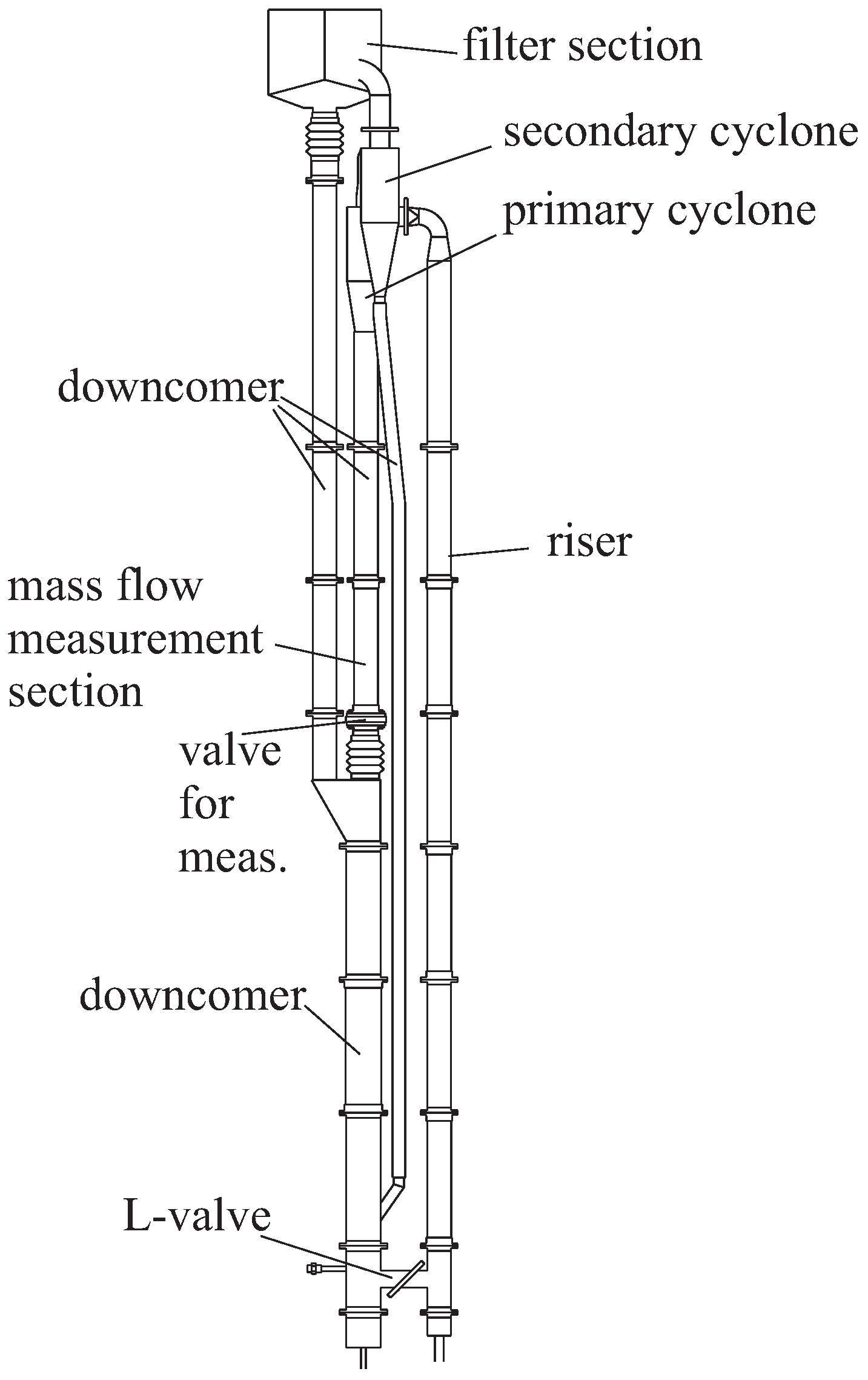
Consider the illustration of a CFB unit depicted in Figure 1. The tall and slender column within the equipment is commonly known as the riser reactor. Gas moving upwards causes solid particles to become fluidized in the lower section of the riser. The gas–solid flow within a riser is quite diverse, leading to variations in particle concentration both axially and radially. Empirical observations have indicated that solid holdup decreases along the axial direction of a riser [2]. The void fraction throughout the riser is influenced not only by operational conditions and particle characteristics but also by its geometric design. Additionally, void fraction profiles along a riser may exhibit an S-shaped or C-shaped pattern, which heavily depends on inlet and outlet configurations [3]. Riser units typically operate under fast fluidization conditions, characterized by dilute particle flow at its core and dense annular regions (particle clusters) along its walls, a phenomenon referred to as core–annular flow [4]. Due to the intricate hydrodynamics involved in CFB units, their design process has historically relied heavily on empirical correlations derived from experience. With advancements in computing capabilities, computational fluid dynamics has emerged as an essential tool for simulating complex multiphase flows such as gas–solid interactions within risers; however, experimental data remain crucial for validation purposes.

In the realm of computer simulations for gas–solid flows, there exist two potential methods for handling the solid phase. The Lagrangian approach involves representing the solid phase with a finite number of particles whose movement is monitored in both space and time. When particle concentration reaches a certain level, it becomes important to account for particle collisions and interactions with the fluid. This method is most suitable for modeling gas–solid flow when the particle concentration is low or dilute [6,7,8]. The Lagrangian approach provides information on individual particle trajectories, velocities, and interactions, allowing for a more accurate representation of the solid phase. However, as particle concentration increases, keeping track of individual particles, their collisions, and interactions with the fluid becomes computationally demanding, which necessitates an alternative framework. Conversely, the Eulerian approach is a continuum-based model that treats the solid phase as a quasi-fluid possessing properties similar to those of the primary phase (the gas). This methodology is best suited for situations where there is high particle concentration such as in industrial scale equipment [9]. Rather than dealing with particles individually, this framework averages out their motion while treating both solid and gas phases as interpenetrating continuums—also known as Eulerian–Eulerian or two-fluid model [10,11,12,13]. The E-E model has significantly lower computational demands compared to tracking a large number of individual particles using the Lagrangian methodology and monitoring each one’s movement separately. E-E excels particularly well in managing dense flows marked by frequent occurrences of particle interactions alongside permanent contact between particles. A monodispersed particle size distribution (single-particle mean diameter) is commonly assumed to simplify the mathematical description of the solid phase in favor of this approach. E-E model simulations capture macroscopic behaviors such as gas- and solid-phase distributions and the velocity field of each phase, which is essential information in many engineering applications. In the current study, the Eulerian–Eulerian approach is employed to simulate the gas–solid flow within the CFB riser.

The two-fluid model does not resolve the individual motion of particles; the averaging of microscopic interactions creates a challenge in defining the interphase momentum exchange (drag force) and modeling the solid-phase stress tensor. The success of the E-E approach largely relies on accurate closure models able to represent all relevant interaction forces. Drag force models, often based on experimental data under uniform conditions, are frequently utilized in simulating fluidized beds [14,15,16]. These models usually work well in zones of low particle concentration, i.e., dilute flow, where homogeneous conditions are satisfied [17]. The energy-minimization multi-scale drag model has proven effective in predicting axial solid distribution and core–annular flow structures in riser simulations by considering meso-scale structures commonly observed in fluidization technology [18,19]. The core principle of the EMMS framework is to minimize the energy required for particle transport and suspension. As particle concentration rises, particles naturally form clusters to decrease fluid flow resistance. Consequently, the fluid bypasses these clusters rather than flowing through them. The EMMS drag model accounts for key mechanisms seen in circulating fluidized beds such as interactions between gas and particles in both dense cluster and dilute states, along with interaction between dense clusters and dilute regions. The EMMS model introduces a correction factor that reduces the drag coefficient ($C_D$) when particle clusters form, making it suitable for approximating flow patterns observed in a CFB riser. A model for predicting the heterogeneous flow structure parameters within the EMMS framework was proposed by Hou et al. [20] that seems to improve the prediction of axial distribution of average voidage in a 2D riser. Qi et al. [17] also adopted the EMMS theory to account for the cluster effect in their riser simulations. They did not consider gas-phase turbulence, asserting that it is of minor importance in dense flow simulations. Solid-phase stress tensor closures are typically derived from the kinetic theory of granular flow [11,21]. The stress tensor in the solid phase is proportionally related to the mean velocity gradients. By expressing solid-phase viscosities in terms of the mean particle diameter, volume fraction, and fluctuating kinetic energy (granular temperature), the equation set can be effectively closed.

The E-E model has been widely used to simulate the gas–solid flow in risers of different configurations. This type of multiphase flow is inherently three-dimensional (3D), time-dependent, and turbulent. Nevertheless, prior numerical simulations have opted for simplifications, modeling the gas–solid flow in a riser as two-dimensional (2D) flow [20,22,23,24]. While these simplified simulations managed to capture either the axial or radial solid distributions, it was observed that the 2D domains constrained particle motion in the transverse direction, therefore leading to results of solid holdup that are not entirely accurate. The recent works have also featured additional simplifications, such as neglecting turbulence in the gas phase [25,26,27,28]. Li et al.’s comparison of axial pressure gradients and radial solid concentration profiles obtained from both 2D and 3D simulations in CFB risers with square and circular cross-sections showed that square cross-section predictions from 2D simulations resulted in significantly lower axial pressure gradients—a measure of axial solid distribution; no axisymmetric behavior was observed for their 2D cylindrical riser simulation results [29]. They demonstrated that due to removing the third coordinate direction, matching both axial pressure gradient and radial solid concentration profiles using only two dimensions is not feasible for simulating CFB risers.

Shah et al. [23] studied the impact of different models on predicting solid distribution in a riser, including the interphase drag force model and the gas-phase stress model. They found that the partial-slip wall-boundary condition for the solid phase significantly affects predictions of axial and radial profiles of solid concentration. The study concluded that this boundary condition is flow-dependent, with major discrepancies at low solid flux. Additionally, they discussed using specularity coefficient as a criterion to prescribe momentum conservation equation at the wall, reporting values from 0.1 to 0.0001 as providing reasonable results. The EMMS drag model was also highlighted for its significant influence on predicting radial solid-phase volume fraction, showing good agreements, especially at high solid flux levels. On the other hand, the 2D fluidized bed simulations performed by Venier et al. [28] showed that a no-slip condition ($\phi =1$) in combination with an adjusted Di Felice drag model [30] led to better predictions of solid-phase velocity for a wide range of fluidization conditions. Consequently, there is little consensus on the appropriate value for the specularity coefficient, leaving it as a parameter that must be tuned in riser simulations.

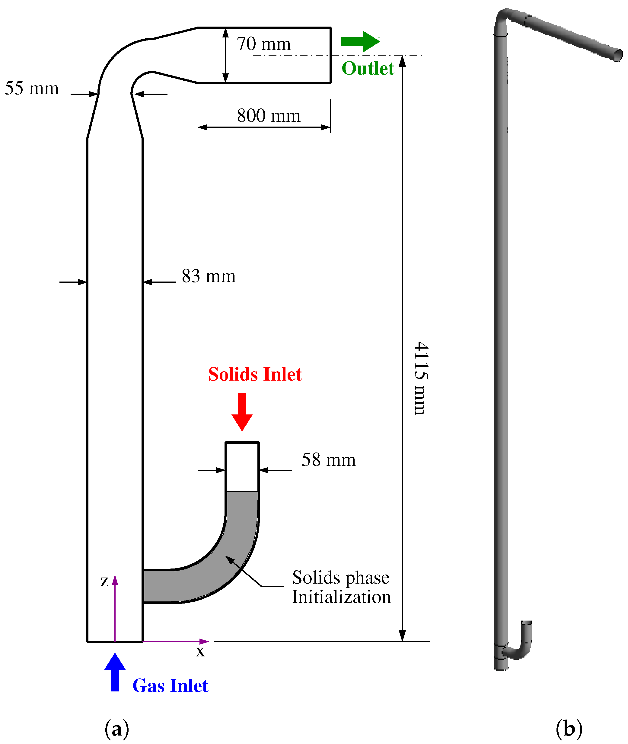
Despite the extensive research, it is crucial to analyze the influence of drag models on various three-dimensional flow conditions, variations in CFB-riser design, and specific characteristics of particulate matter. This study investigates the impact of three different drag models on the predictions of axial and radial solid-phase volume fraction in a CFB riser. The analysis also includes examining the effects of a three-dimensional domain configuration, time-averaging, and turbulence modulation on solid concentration within the riser. In the computational approach proposed here, RANS turbulence models with additional modulation terms are used to approximate two-way coupling effects at fluctuation levels, a feature seldom integrated into or implemented in two-phase flow simulations of CFB riser. An interesting finding of this study is that employing the k-$\omega$ SST turbulence model without modulation terms yields comparable results for solid-phase distribution in the dilute section of the riser as those obtained with the k-$ϵ$ model. The solid-phase transport equations incorporate the full granular temperature equation and constitutive relations derived from the kinetic theory of granular flow, as well as the departure from a semi-empirical model for frictional viscosity. To our knowledge, no previous work has covered all these mechanisms examined in this study concerning CFB risers. The commercial CFD software ANSYS-Fluent 2022R2 is employed for solving two-fluid model equations. The simulation results are compared with the experimental measurements obtained from five different elevations along the riser [5] to provide a quantitative assessment of the investigated drag models in terms of the root mean square error.

2. Methods

2.1. Experimental Rig

The assessment of particle concentration in CFB units has been conventionally centered around measurements in risers featuring a squared cross-sectional geometry [2,31]. Reliable experimental measurements conducted in risers with a circular cross-section are relatively scarce in the literature. The CFB unit shown in Figure 1 corresponds to a schematic of the cold-CFB test unit used at Delft University of Technology; this facility shares similarities with other CFB units employed in various experimental campaigns [26,32,33]. Professor Rudd van Ommen led an experimental campaign to measure the axial pressure gradient and radial solid concentration in the riser depicted in Figure 1 [5]. The experimental setup consists of a stainless steel riser with a circular cross-section of 83 mm and a height of approximately 4 m. This riser is larger and wider than the one described by Mathiesen et al. [32] but shorter and more slender than the riser researched by Malcus et al. [34]. The single-loop CFB unit in Figure 1 is equipped with a porous plate gas distributor. The solids enter laterally at the bottom of the riser and are fluidized by the upward airflow. Primary and secondary cyclones separate the gas from the solids. A downcomer returns solids to the bottom of the riser. The downcomer operates as a moving bed to recirculate the material back to the riser via an L-valve. Several compartments of the riser are made of glass to facilitate visual inspection. Further details of the CFB unit and its operation can be found in [35].

The average pressure drop along the riser was determined by using pressure taps placed at eleven positions above the gas distributor. Druck pressure sensors type PMP 4165 were used to measure the pressure drop at each pair of adjacent pressure taps. The average was taken over 8 min. The pressure drop measurements along the riser serve as an indirect means to estimate the axial solid-phase concentration [36]. Optical probes of the reflection type were used to determine the radial solid concentration profiles at five different heights above the distributor. The probes consist of sending and receiving elements placed at the tip of a tube of 5 mm diameter. The measurements obtained with this type of probe may exhibit lower accuracy compared to non-intrusive techniques [37], such as particle-image velocimetry (PIV), which are also suitable for investigating particle clusters [38]. The probes were first deeply inserted in the riser to measure the voidage, i.e., the fraction of the total volume available for the gas to flow through, near the opposite riser surface. The probes were then traversed across the riser diameter in steps of 5 mm, and signals were recorded for 2 min at every position. The average voidage was determined from such measurements. The solid mass-flux was measured at a transparent section of the downcomer [5].

2.2. Computational Model

The two-phase flow E-E model is implemented in ANSYS-Fluent software version 2022R2 to compute the gas- and solid-phase flow in the riser of the cylindrical cold CFB unit shown in Figure 1. A symmetry plane of the corresponding computational domain is depicted in Figure 2a, indicating the main dimensions taken from the actual riser in the unit. The computational domain shown in Figure 2b features a full cylindrical 3D geometry, although one case was simulated as two-dimensional (2D) by just taking the center plane of the riser. The gas flow enters the bottom of the riser in plug flow, and a short elbow attached to the riser is used to feed the solids, resembling the way particles are conveyed from the downcomer to the riser in the actual CFB unit. Special care was taken to accurately model the riser exit geometry; at the upper section of the riser, the gas–solid flow passes through a gradual contraction, a ${90}^{\circ }$ bend, and a diffuser before exiting the domain through a 70 mm diameter pipe, as can be seen in Figure 2a. This configuration resembles a smooth C-type exit, as described by Shi et al. [39], facilitating the flow of particles out of the riser. Typically, the riser exit geometry has been simplified to a straight outlet in various numerical simulations [22,32,40,41]. Nevertheless, there is evidence that the exit layout can have a significant effect on both local and overall solid hydrodynamics in the riser [42]. The previous studies indicate that the exit effect is more important in risers of circular and square cross-sections [43], underscoring the importance of accurately accounting for their geometric details.

Gas- and solid-phase properties are listed in

Table 1. Cold-CFB riser parameters.

Riser	Diameter, D	83 mm
	Height, H	4.1 m
Solid phase	Particle mean diameter, $d_s$	$410\mathsf{\mu }$m
	Particle density, ${\rho }_s$	2600 kg/m3
Gas phase	Gas density, ${\rho }_g$	$1.225$ kg/m3
	Gas viscosity, ${\mu }_g$	$1.8\times {10}^{-5}$ kg/m·s
Flow condition	Superficial gas velocity, $U_0$	5 m/s
	solid flux	40 kg/m2·s

. The solid phase is considered monodispersed, whose mean diameter indicates that particles belong to the Geldart B group [44]. The superficial gas velocity is specified at the inlet boundary for the gas phase. This velocity is much larger than the minimum fluidization velocity (0.16 m/s) determined with the empirical correlation proposed by Grace [9]. Governing equations of the E-E model are presented in Table 2. In the two-fluid model, the conservation equations for the gas phase incorporate the effect of the particles through the volume fraction (${\varphi }_g=1-{\varphi }_s$) and the interphase momentum exchange terms. Volume conservation requires that gas and solid volume fractions sum up to unity. In this work, the mean drag force proportional to the relative velocity $\left({\overrightarrow{V}}_g-{\overrightarrow{V}}_s\right)$ is considered as the main momentum exchange term between the phases. The employed drag model correlations strongly depend on volume fraction and the flow regime, characterized by the particle Reynolds number,

$$R{e}_s=\frac{{\rho }_g{d}_s\left|{\overrightarrow{V}}_s-{\overrightarrow{V}}_g\right|}{{\mu }_g}$$

(1)

The dispersed k-$\omega$ SST turbulence model is chosen to account for turbulence in the gas phase for most of the simulated cases. While most CFD simulations on gas–solid flow in risers have used k-$ϵ$ turbulence models, the less common k-$\omega$ SST model has consistently shown better predictive abilities for different flow conditions [45]. With its potential to provide a more precise representation of the near-wall region with adequately refined grid resolution, the inclusion of the k-$\omega$ SST model can help effectively capture gas–solid interactions and cluster dynamics close to the riser wall. The turbulence model includes the modulation term, ${\mathrm{\Pi }}_k$, in the transport equation for turbulence kinetic energy [46],

$${\mathrm{\Pi }}_k={\beta }_{sg}\left[k_{sg}-2k-\left({\overrightarrow{V}}_g-{\overrightarrow{V}}_s\right)·{\overrightarrow{V}}_{dr}\right]$$

(2)

The drift velocity ${\overrightarrow{V}}_{dr}$ accounts for the correlation between the instantaneous distribution of particles and the turbulent fluid motion at scales larger than the particle diameter. It is also needed to compute the turbulence dispersion force ${\overrightarrow{F}}_{td}$ in the momentum conservation equations (Table 2). It is customary to model the drift velocity as proportional to gradients of volume fraction and introduce a turbulent dispersion coefficient (${\mathcal{D}}_{sg}$) that depends on the covariance of gas and solid velocity fluctuations, $k_{sg}$. Closure models for the drift velocity and other correlations are grouped in

Table A3. Turbulence closures.

Turbulence dispersion force  [21], used in Equations (6) and (7), Table 2, $${\displaystyle {\overrightarrow{F}}_{td}=-{\beta }_{sg}{\overrightarrow{V}}_{dr}}$$ (A17)

Covariance of gas-phase and solid-phase velocity fluctuations, $k_{sg}$ [21],

used in Equation (2)

$${\displaystyle k_{sg}=2k\left(\frac{\chi +\eta }{1+\eta }\right),\mathrm{with}\chi =\left(1+C_v\right){\left(\frac{{\rho }_s}{{\rho }_g}+C_v\right)}^{-1},\mathrm{and}\eta =\frac{{\tau }_{t,sg}}{{\tau }_{F,sg}}}$$ (A18)

Drift velocity [21,46] used in Equation (2), $${\displaystyle {\overrightarrow{V}}_{dr}=-\frac{{\mathcal{D}}_{sg}}{{\sigma }_{sg}}\left(\frac{1}{{\varphi }_s}\nabla {\varphi }_s-\frac{1}{{\varphi }_g}\nabla {\varphi }_g\right),\mathrm{with}{\mathcal{D}}_{sg}=\frac{1}{3}{k}_{sg}{\tau }_{t,sg}}$$ (A19)

Lagrangian integral time-scale calculated along particle trajectories [21]

$${\displaystyle {\tau }_{t,sg}=\frac{{\tau }_{t,g}}{\sqrt{1+C_{\beta }{\xi }^2}},\mathrm{with}{C}_{\beta }=1.8-1.35{cos}^2{\theta }_t,\mathrm{and}\xi =\frac{\left|{\overrightarrow{V}}_g-{\overrightarrow{V}}_s\right|{\tau }_{t,g}}{L_{t,g}}}$$ (A20)

${\theta }_t$ is the angle between the mean particle velocity and the mean relative velocity.

Particle relaxation time due to inertial effects acting on the solid phase [21] $${\displaystyle {\tau }_{F,sg}=\frac{{\varphi }_s{\rho }_s}{{\beta }_{sg}}\left(\frac{{\rho }_s}{{\rho }_g}+C_v\right)}$$ (A21)

Characteristic turbulent time-scale ${\displaystyle {\tau }_{t,g}=\frac{3}{2}{b}^{*}{\omega }^{-1}}$ and Characteristic turbulent length-scale ${\displaystyle L_{t,g}=\sqrt{\frac{3}{2}}{b}^{*}\frac{\sqrt{k}}{\omega }}$

Turbulent viscosity [59], $${\displaystyle {\mu }_t=\frac{{\rho }_{g}k/\omega }{max\left[\frac{1}{{\alpha }^{*}},\frac{Stanh\left({\zeta }_2^2\right)}{a_1\omega }\right]},\mathrm{with}{\zeta }_2=max\left[\frac{2\sqrt{k}}{0.09\omega y},\frac{500{\mu }_g}{{\rho }_g{y}^2\omega }\right]}$$ (A22)

y is the distance to the next surface.

Gas-phase mean rate of strain tensor, $${\displaystyle S=\sqrt{\frac{1}{2}\left(\nabla {\overrightarrow{V}}_g+\nabla {\overrightarrow{V}}_g^T\right):\left(\nabla {\overrightarrow{V}}_g+\nabla {\overrightarrow{V}}_g^T\right)}}$$ (A23)

Turbulent Prandtl numbers for k and $\omega$ [59], $${\displaystyle {\sigma }_k=\frac{1}{\frac{tanh{\zeta }_1^4}{{\sigma }_{k,1}}+\frac{1-tanh{\zeta }_1^4}{{\sigma }_{k,2}}}\mathrm{and}{\sigma }_{\omega }=\frac{1}{\frac{tanh{\zeta }_1^4}{{\sigma }_{\omega ,1}}+\frac{1-tanh{\zeta }_1^4}{{\sigma }_{\omega ,2}}}}$$ (A24)

with ${\displaystyle {\zeta }_1=min\left[max\left(\frac{\sqrt{k}}{0.09\omega y},\frac{500{\mu }_g}{{\rho }_g{y}^2\omega }\right),\frac{4{\rho }_{g}k}{{\sigma }_{\omega ,2}{D}_{\omega }^{+}{y}^2}\right],}$ ${\displaystyle D_{\omega }^{+}=max\left[2{\rho }_g\frac{1}{{\sigma }_{\omega ,2}}\frac{1}{\omega }\left(\nabla k·\nabla \omega \right),{10}^{-10}\right]}$

Cross diffusion term [59], $${\displaystyle D_{\omega }=\frac{2\left(1-tanh{\zeta }_1^4\right)}{{\sigma }_{\omega ,2}\omega }\left(\nabla k·\nabla \omega \right)}$$ (A25)

Turbulence modeling functions and constants

${\displaystyle f_{\omega }={\alpha }_{\infty }\left(\frac{{\alpha }_0+R{e}_t/R_{\omega }}{1+R{e}_t/R_{\omega }}\right),}$ ${\alpha }_{\infty }={\alpha }_{\infty ,1}tanh{\zeta }_1^4+{\alpha }_{\infty ,2}\left(1-tanh{\zeta }_1^4\right),$ ${\displaystyle {\alpha }_0=\frac{1}{9},{\alpha }^{*}=1}$

${\displaystyle {\alpha }_{\infty ,1}=\frac{b_1}{b^{*}}-\frac{{\kappa }^2}{{\sigma }_{\omega ,1}\sqrt{b^{*}}},}$${\displaystyle {\alpha }_{\infty ,2}=\frac{b_2}{b^{*}}-\frac{{\kappa }^2}{{\sigma }_{\omega ,2}\sqrt{b^{*}}},}$$b_i=b_{1}tanh{\zeta }_1^4+b_2\left(1-tanh{\zeta }_1^4\right)$

${\displaystyle R{e}_t=\frac{{\rho }_{g}k}{{\mu }_g\omega },}$${\sigma }_{k,1}=1.176$${\sigma }_{k,2}=1.0$${\sigma }_{\omega ,1}=2.0$${\sigma }_{\omega ,2}=1.168$${\sigma }_{sg}=0.75$$C_v=0.5$

$b_1=0.075$$b_2=0.0828$$b^{*}=0.09$$R_{\omega }=2.95$$a_1=0.31$$C_3=1.2$$\kappa =0.41$

in the Appendix A. The effect of the solid phase on the specific dissipation rate equation [47],

$${\mathrm{\Pi }}_{\omega }=C_3\omega {\mathrm{\Pi }}_k$$

(3)

Table 2. Governing equations of the E-E model. Closure relations for the general interphase momentum transfer coefficient (${\beta }_{sg}$), turbulence dispersion force (${\overrightarrow{F}}_{td}$), collisional dissipation (${\gamma }_s$), and others are found in

Table A1. Constitutive relations of the Euler–Euler model.

Laminar flow stress tensor, used in Equation (6), Table 2	$${\overline{\overline{\tau }}}_{g,l}={\mu }_g\left[\left(\nabla {\overrightarrow{V}}_g+\nabla {\overrightarrow{V}}_g^T\right)-\frac{2}{3}\left(\nabla ·{\overrightarrow{V}}_g\right)\overline{\overline{I}}\right]$$ (A1)
Turbulent flow stress tensor, used in Equation (6), Table 2	$${\overline{\overline{\tau }}}_{g,t}={\mu }_t\left(\nabla {\overrightarrow{V}}_g+\nabla {\overrightarrow{V}}_g^T\right)-\frac{2}{3}{\rho }_{f}k\overline{\overline{I}}$$ (A2)
solid shear stress tensor, used in Equation (7), Table 2	$${\overline{\overline{\tau }}}_s={\mu }_s\left(\nabla {\overrightarrow{V}}_s+\nabla {\overrightarrow{V}}_s^T\right)-\left({\lambda }_s-\frac{2}{3}{\mu }_s\right)\left(\nabla ·{\overrightarrow{V}}_s\right)\overline{\overline{I}}$$ (A3)
solid-phase pressure [48], used in Equations (7) and (10), Table 2	$$P_s={\varphi }_s{\rho }_s{\mathrm{\Theta }}_s+2{\rho }_s\left(1+e_s\right){\varphi }_s^2{g}_0{\mathrm{\Theta }}_s$$ (A4)
solid-phase viscosity	$${\mu }_s={\mu }_{s,c}+{\mu }_{s,k}+{\mu }_{s,f}$$ (A5)
solid collisional viscosity [16]	$${\mu }_{s,c}=\frac{4}{5}{\varphi }_s^2{\rho }_s{d}_s{g}_0\left(1+e_s\right)\sqrt{\frac{{\mathrm{\Theta }}_s}{\pi }}$$ (A6)
solid kinetic viscosity [16]	$${\mu }_{s,k}=\frac{10{\rho }_s{d}_s\sqrt{\pi {\mathrm{\Theta }}_s}}{96{\varphi }_s\left(1+e_s\right)g_0}{\left[1+\frac{4}{5}{g}_0{\varphi }_s\left(1+e_s\right)\right]}^2$$ (A7)
solid frictional viscosity [57], used only in Equation (7), Table 2	$${\mu }_{s,f}=\frac{P_{s}sin\delta }{2\sqrt{I_{2D}+{\mathrm{\Theta }}_s/d_s^2}}$$ (A8)
	$I_{2D}$ is the second invariant of the deviatoric strain-rate tensor.
solid bulk viscosity [48]	$${\lambda }_s=\frac{4}{3}{\varphi }_s^2{\rho }_s{d}_s{g}_0\left(1+e_s\right)\sqrt{\frac{{\mathrm{\Theta }}_s}{\pi }}$$ (A9)
solid conductivity [16], used in Equation (10), Table 2	$${\kappa }_s=\frac{150{\rho }_s{d}_s\sqrt{\pi {\mathrm{\Theta }}_s}}{384\left(1+e_s\right)g_0}{\left[1+\frac{6}{5}{\varphi }_s{g}_0\left(1+e_s\right)\right]}^2+2{\rho }_s{\varphi }_s^2{d}_s\left(1+e_s\right)g_0\sqrt{\frac{{\mathrm{\Theta }}_s}{\pi }}$$ (A10)
Collisional dissipation of ${\mathrm{\Theta }}_s$ [48], used in Equation (10), Table 2	$${\gamma }_s=\frac{12\left(1-e_s^2\right)g_0}{d_s\sqrt{\pi }}{\rho }_s{\varphi }_s^2{\mathrm{\Theta }}_s^{3/2}$$ (A11)
Radial distribution function [58]	$$g_0={\left[1-{\left(\frac{{\varphi }_s}{{\varphi }_{s,max}}\right)}^{1/3}\right]}^{-1}$$ (A12)
General interphase momentum transfer coefficient	$${\beta }_{sg}=\frac{3}{4}{C}_D\frac{{\varphi }_s{\varphi }_g^n{\rho }_g\left|{\overrightarrow{V}}_s-{\overrightarrow{V}}_g\right|}{q^2{d}_s}{H}_D$$ (A13)

and Table A3 in the Appendix A.

Continuity equation for gas phase

$${\displaystyle \frac{\partial }{\partial t}\left({\varphi }_g{\rho }_g\right)+\nabla ·\left({\varphi }_g{\rho }_g{\overrightarrow{V}}_g\right)=0}$$ (4)

Volume fraction

$${\varphi }_g+{\varphi }_s=1$$ (5)

Momentum conservation equation for gas phase

$${\displaystyle \frac{\partial }{\partial t}\left({\varphi }_g{\rho }_g{\overrightarrow{V}}_g\right)+\nabla ·\left({\varphi }_g{\rho }_g{\overrightarrow{V}}_g{\overrightarrow{V}}_g\right)=-{\varphi }_g\nabla P+{\varphi }_g\nabla ·\left({\overline{\overline{\tau }}}_{g,l}+{\overline{\overline{\tau }}}_{g,t}\right)+{\varphi }_g{\rho }_g\overrightarrow{g}-{\beta }_{sg}\left({\overrightarrow{V}}_g-{\overrightarrow{V}}_s\right)+{\overrightarrow{F}}_{td}}$$ (6)

Momentum conservation equation for solid phase

$${\displaystyle \frac{\partial }{\partial t}\left({\varphi }_s{\rho }_s{\overrightarrow{V}}_s\right)+\nabla ·\left({\varphi }_s{\rho }_s{\overrightarrow{V}}_s{\overrightarrow{V}}_s\right)=-{\varphi }_s\nabla P-\nabla P_s+\nabla ·{\overline{\overline{\tau }}}_s+{\varphi }_s{\rho }_s\overrightarrow{g}+{\beta }_{sg}\left({\overrightarrow{V}}_g-{\overrightarrow{V}}_s\right)-{\overrightarrow{F}}_{td}}$$ (7)

k-$\omega$ SST dispersed turbulence model

$${\displaystyle \frac{\partial }{\partial t}\left({\varphi }_g{\rho }_{g}k\right)+\nabla ·\left({\varphi }_g{\rho }_g{\overrightarrow{V}}_{g}k\right)=\nabla ·\left[{\varphi }_g\left({\mu }_g+\frac{{\mu }_t}{{\sigma }_k}\right)\nabla k\right]+{\varphi }_g{\overline{\overline{\tau }}}_{g,t}:\nabla {\overrightarrow{V}}_g-{\varphi }_g{\rho }_g\left(b^{*}k\omega -{\mathrm{\Pi }}_k\right)}$$ (8)

$${\displaystyle \frac{\partial }{\partial t}\left({\varphi }_g{\rho }_g\omega \right)+\nabla ·\left({\varphi }_g{\rho }_g{\overrightarrow{V}}_g\omega \right)=\nabla ·\left[{\varphi }_g\left({\mu }_g+\frac{{\mu }_t}{{\sigma }_{\omega }}\right)\nabla \omega \right]+{\varphi }_g{\rho }_g\left[\frac{f_{\omega }}{{\mu }_t}\left({\overline{\overline{\tau }}}_{g,t}:\nabla {\overrightarrow{V}}_g\right)-b_i{\omega }^2+D_{\omega }+{\mathrm{\Pi }}_{\omega }\right]}$$ (9)

Granular temperature equation

$${\displaystyle \frac{3}{2}\left[\frac{\partial }{\partial t}\left({\varphi }_s{\rho }_s{\mathrm{\Theta }}_s\right)+\nabla ·\left({\varphi }_s{\rho }_s{\overrightarrow{V}}_s{\mathrm{\Theta }}_s\right)\right]=\nabla ·\left({\kappa }_s\nabla {\mathrm{\Theta }}_s\right)+\left[-P_s\overline{\overline{I}}+\left({\overline{\overline{\tau }}}_{s,c}+{\overline{\overline{\tau }}}_{s,k}\right)\right]:\nabla {\overrightarrow{V}}_s-{\gamma }_s-3{\beta }_{sg}{\mathrm{\Theta }}_s}$$ (10)

Table 2. Governing equations of the E-E model. Closure relations for the general interphase momentum transfer coefficient (${\beta }_{sg}$), turbulence dispersion force (${\overrightarrow{F}}_{td}$), collisional dissipation (${\gamma }_s$), and others are found in Table A1 and Table A3 in the Appendix A.

Continuity equation for gas phase

$${\displaystyle \frac{\partial }{\partial t}\left({\varphi }_g{\rho }_g\right)+\nabla ·\left({\varphi }_g{\rho }_g{\overrightarrow{V}}_g\right)=0}$$ (4)

Volume fraction

$${\varphi }_g+{\varphi }_s=1$$ (5)

Momentum conservation equation for gas phase

$${\displaystyle \frac{\partial }{\partial t}\left({\varphi }_g{\rho }_g{\overrightarrow{V}}_g\right)+\nabla ·\left({\varphi }_g{\rho }_g{\overrightarrow{V}}_g{\overrightarrow{V}}_g\right)=-{\varphi }_g\nabla P+{\varphi }_g\nabla ·\left({\overline{\overline{\tau }}}_{g,l}+{\overline{\overline{\tau }}}_{g,t}\right)+{\varphi }_g{\rho }_g\overrightarrow{g}-{\beta }_{sg}\left({\overrightarrow{V}}_g-{\overrightarrow{V}}_s\right)+{\overrightarrow{F}}_{td}}$$ (6)

Momentum conservation equation for solid phase

$${\displaystyle \frac{\partial }{\partial t}\left({\varphi }_s{\rho }_s{\overrightarrow{V}}_s\right)+\nabla ·\left({\varphi }_s{\rho }_s{\overrightarrow{V}}_s{\overrightarrow{V}}_s\right)=-{\varphi }_s\nabla P-\nabla P_s+\nabla ·{\overline{\overline{\tau }}}_s+{\varphi }_s{\rho }_s\overrightarrow{g}+{\beta }_{sg}\left({\overrightarrow{V}}_g-{\overrightarrow{V}}_s\right)-{\overrightarrow{F}}_{td}}$$ (7)

k-$\omega$ SST dispersed turbulence model

$${\displaystyle \frac{\partial }{\partial t}\left({\varphi }_g{\rho }_{g}k\right)+\nabla ·\left({\varphi }_g{\rho }_g{\overrightarrow{V}}_{g}k\right)=\nabla ·\left[{\varphi }_g\left({\mu }_g+\frac{{\mu }_t}{{\sigma }_k}\right)\nabla k\right]+{\varphi }_g{\overline{\overline{\tau }}}_{g,t}:\nabla {\overrightarrow{V}}_g-{\varphi }_g{\rho }_g\left(b^{*}k\omega -{\mathrm{\Pi }}_k\right)}$$ (8)

$${\displaystyle \frac{\partial }{\partial t}\left({\varphi }_g{\rho }_g\omega \right)+\nabla ·\left({\varphi }_g{\rho }_g{\overrightarrow{V}}_g\omega \right)=\nabla ·\left[{\varphi }_g\left({\mu }_g+\frac{{\mu }_t}{{\sigma }_{\omega }}\right)\nabla \omega \right]+{\varphi }_g{\rho }_g\left[\frac{f_{\omega }}{{\mu }_t}\left({\overline{\overline{\tau }}}_{g,t}:\nabla {\overrightarrow{V}}_g\right)-b_i{\omega }^2+D_{\omega }+{\mathrm{\Pi }}_{\omega }\right]}$$ (9)

Granular temperature equation

$${\displaystyle \frac{3}{2}\left[\frac{\partial }{\partial t}\left({\varphi }_s{\rho }_s{\mathrm{\Theta }}_s\right)+\nabla ·\left({\varphi }_s{\rho }_s{\overrightarrow{V}}_s{\mathrm{\Theta }}_s\right)\right]=\nabla ·\left({\kappa }_s\nabla {\mathrm{\Theta }}_s\right)+\left[-P_s\overline{\overline{I}}+\left({\overline{\overline{\tau }}}_{s,c}+{\overline{\overline{\tau }}}_{s,k}\right)\right]:\nabla {\overrightarrow{V}}_s-{\gamma }_s-3{\beta }_{sg}{\mathrm{\Theta }}_s}$$ (10)

The turbulence model parameters needed to compute ${\mathrm{\Pi }}_k$ and ${\mathrm{\Pi }}_{\omega }$ are summarized in Table A3. To assess the sensitivity of results to turbulence modeling, the standard k-$ϵ$ model was exclusively applied in Case 9 as part of the evaluation process, as it is highlighted in

Table 3. Summary of CFB-riser simulations.

Case	Number of Cells	Geometry	Drag Model	Turbulence Modulation Equations (2) and (3)
1	$1.9\times {10}^4$	2D	EMMS [19]	yes
2	$7.0\times {10}^4$	3D	EMMS	yes
3	$1.4\times {10}^5$	3D	EMMS	yes
4	$2.9\times {10}^5$	3D	Wen–Yu [14]	yes
5	$2.9\times {10}^5$	3D	EMMS	yes
6	$2.9\times {10}^5$	3D	Syamlal–O’Brien [15]	yes
7	$2.9\times {10}^5$	3D	EMMS	no
8	$2.7\times {10}^6$	3D	EMMS	yes
9	$2.9\times {10}^5$	3D	EMMS	yes, k-$ϵ$ model

. The standard k-$ϵ$ model incorporates similar modulation terms to those given by Equations (2) and (3). The energy associated with particle velocity fluctuations is modeled by considering a transport equation for the granular temperature (${\mathrm{\Theta }}_s=\langle v_s{v}_s\rangle /3$) in the solid phase. The closure relations from kinetic theory of granular flow [11,48,49] are used to specify pressure, kinetic and collisional viscosity coefficients, bulk viscosity, conductivity, radial distribution function, and collisional dissipation in the solid phase. These closure relations are provided in Appendix A (Table A1). The E-E model also incorporates a frictional viscosity (${\mu }_{s,f}$) to account for long and permanent particle contact when the solid-phase volume fraction is greater than a threshold value (${\varphi }_{s,max}$). The expression of solid frictional viscosity usually adopts a frictional pressure framework borrowed from soil mechanics. It incorporates empirical parameters that require fine-tuning based on the bed material (such as the angle of internal friction, $\delta$ in

Table 4. Modeling parameters and simulation settings.

Parameter	Value
Inter-particle restitution coefficient, $e_s$	$0.9$
Particle–wall restitution coefficient, $e_w$	$0.9$
Specularity coefficient, $\phi$	$0.005$
Maximum packing limit, ${\varphi }_{s,max}$	$0.63$
Friction packing limit, ${\varphi }_{s,min}$	$0.5$
Angle of internal friction, $\delta$	${28}^{\circ }$
Pressure–velocity coupling	Phase-coupled SIMPLE
Pressure discretization	PRESTO!
Momentum discretization	Second-order upwind
Volume fraction discretization	QUICK
Turbulence discretization	Second-order upwind
Granular temperature	First-order upwind
Unsteady formulation	Bounded second-order implicit
Convergence criteria	10−4
Time step	0.0001 s

) and the fluidization regime [50]. In this work, the closure relation for the solid frictional viscosity does not incorporate an empirical equation for normal frictional stresses [12]; instead, the solid-phase pressure derived from the kinetic theory of granular flow is adopted as the normal frictional stress, so a custom implementation of the frictional viscosity was required in the commercial software used. Although the full solid shear stress tensor acts in the momentum conservation equation for the solid phase, the kinetic and collisional viscosities (${\mu }_{s,k}$ and ${\mu }_{s,c}$) are only taken into account to compute the production term in the granular temperature equation (see ${\mathrm{\Theta }}_s$ equation in Table 2).

In this work, three different drag model correlations are evaluated, namely, the Wen and Yu [14] drag model, usually employed to simulate dilute systems; the drag correlation proposed by Syamlal–O’Brien [15], commonly employed in the simulation of Geldart B particles; and the EMMS [19] drag model are used to compute the general interphase momentum transfer coefficient, ${\beta }_{sg}$ (see Table A1 and

Table A2. Drag model correlations.

Wen and Yu  [14]	$${\displaystyle C_D=\frac{24}{{\varphi }_{g}R{e}_s}\left(1+0.15·{\left[{\varphi }_{g}R{e}_s\right]}^{0.687}\right),n=-1.65,q=H_D=1}$$ (A14)
Syamlal–O’Brien  [15]	$${\displaystyle C_D={\left[0.63+4.8\sqrt{q/R{e}_s}\right]}^2,n=H_D=1}$$ (A15)
	where $q=0.5\left[A-0.06R{e}_s+\sqrt{{\left(0.06R{e}_s\right)}^2+0.12R{e}_s\left(2B-A\right)+A^2}\right]$
	$A={\varphi }_g^{4.14}$, $B=\left\{\begin{array}{cc}0.8{\varphi }_g^{1.28},\hfill & \mathrm{if}{\varphi }_g\le 0.85\hfill \\ {\varphi }_g^{2.65},\hfill & \mathrm{if}{\varphi }_g>0.85\hfill \end{array}\right.$
EMMS [19]	$$C_D=\left\{\begin{array}{cc}{\displaystyle \frac{24\left[1+0.15{\left({\varphi }_{g}R{e}_s\right)}^{0.687}\right]}{{\varphi }_{g}R{e}_s},}\hfill & \mathrm{if}{\varphi }_{g}R{e}_s<1000\hfill \\ 0.44,\hfill & \mathrm{if}{\varphi }_{g}R{e}_s\ge 1000\hfill \end{array}\right.$$ (A16)
	where $n=q=1$ and $H_D=a{\left({\varphi }_{g}R{e}_s+b\right)}^c,0.001\le {\varphi }_{g}R{e}_s\le 35$
	If $0.4\le {\varphi }_g\le 0.46$ then $\left\{\begin{array}{c}a=0.8526-\frac{0.5846}{1+{\left({\varphi }_g/0.4325\right)}^{22.6279}}\hfill \\ b=c=0\hfill \end{array}\right.$
	If $0.46\le {\varphi }_g\le 0.545$ then $\left\{\begin{array}{c}a=0.032+\frac{0.7399}{1+{\left({\varphi }_g/0.4912\right)}^{54.4265}}\hfill \\ b=0.00225+\frac{772.0074}{1+{10}^{66.3224\left({\varphi }_g-0.3987\right)}}+\frac{0.02404}{1+{10}^{53.8948\left(0.5257-{\varphi }_g\right)}}\hfill \\ c=0.1705-\frac{0.1731}{1+{\left({\varphi }_g/0.502\right)}^{37.7091}}\hfill \end{array}\right.$
	If $0.545\le {\varphi }_g\le 0.99$ then $\left\{\begin{array}{c}a={\left(2124.956-2142.349{\varphi }_g\right)}^{-0.4896}\hfill \\ b={\left(0.8223-0.1293{\varphi }_g\right)}^{13.031}\hfill \\ c=\frac{{\varphi }_g-1.0013}{-0.06633+9.1391\left({\varphi }_g-1.0013\right)+6.9231{\left({\varphi }_g-1.0013\right)}^2}\hfill \end{array}\right.$
	If $0.99\le {\varphi }_g\le 0.9997$ then $\left\{\begin{array}{c}a=0.4243+\frac{0.88\left[1-\frac{1}{1+exp\left(-\left[{\varphi }_g-0.9989\right]/0.00003\right)}\right]}{1+exp\left[-\left({\varphi }_g-0.9942\right)/0.00218\right]}\hfill \\ b=0.01661+0.2436exp\left[-0.5{\left(\frac{{\varphi }_g-0.9985}{0.00191}\right)}^2\right]\hfill \\ c=0.0825-0.0574exp\left[-0.5{\left(\frac{{\varphi }_g-0.9979}{0.00703}\right)}^2\right]\hfill \end{array}\right.$
	If $0.9997\le {\varphi }_g\le 1$ then $a=1,b=c=0$.

). Even though the drag correlation proposed by Gidaspow [16] has been commonly used in the previous numerical studies of risers and similar reactors [51,52], it was not considered here due to the discontinuity observed at a solid volume fraction of 0.2 [44] and its poor performance found in riser simulations [23]. Turbulence closures and constants are summarized in Table A3. The turbulence dispersion force (${\overrightarrow{F}}_{td}$) in the momentum equations accounts for particle dispersion by the gas-phase turbulent motion. Such effect is approximated by a gradient diffusion model [21]. The expression for ${\overrightarrow{F}}_{td}$ is found in Table A3 in the Appendix A.

2.3. Simulation Setup

The numerical solver parameters used are summarized in Table 3. The segregated phase-coupled SIMPLE algorithm together with high-order schemes were used throughout the iterative process. Note that first-order upwind discretization was only specified for the granular temperature. Using higher-order discretization schemes for this quantity resulted in an oscillating behavior of the residual, and convergence below the specified threshold was difficult to achieve. However, employing high-order schemes in the other equations and incorporating a bounded second-order unsteady formulation notably enhances solution accuracy in contrast to the existing literature methodologies [22]. The pressure staggered (PRESTO!) scheme was selected to compute the pressure at cell face centers. The PRESTO! scheme is particularly effective in scenarios involving strong body forces in the flow, such as the weight of particles. The pressure gradients calculated at cell centers are then used to extrapolate pressure to the cell faces, utilizing a staggered grid approach [53]. The default under-relaxation factors for pressure, body force, momentum, volume fraction, turbulence, and granular temperature were adjusted to overcome convergence issues.

The implemented boundary conditions correspond to the parameters from the experimental campaign carried out with the CFB unit shown in Figure 1 [5]. A uniform velocity magnitude (5 m/s), solid volume fraction of ${10}^{-6}$, and turbulence intensity of 1% were specified at the gas inlet boundary. The solid flux determined in the experiments was used to specify the solid inlet velocity. The 800 mm exit duct shown in Figure 2a was further extended to ensure fully developed flow at the outlet boundary (zero normal gradient). Low values of back flow were specified for the turbulent quantities ($k_{\mathrm{outlet}}=1\times {10}^{-3}$ m²/s², ${\omega }_{\mathrm{outlet}}=1\times {10}^{-3}$ s⁻¹), granular temperature (${\mathrm{\Theta }}_{s,\mathrm{outlet}}=1\times {10}^{-5}$ m²/s²) and solid-phase volume fraction (${\varphi }_{s,\mathrm{outlet}}=1\times {10}^{-6}$). Back flow through a few cell faces of the outlet boundary was only observed during the initial stage of the simulations. The partial-slip wall boundary condition proposed by Johnson and Jackson [54] was specified for the solid phase. Following recommendations of the previous studies [11,23,26], a constant specularity coefficient much less than 1 was chosen, as well as fixed values for the restitution coefficients of the particle–wall and inter-particle collisions. Hybrid initialization was used to initialize the flow variables, and the solid volume fraction in the feeding elbow was set to $0.3$, which is represented by the shaded area in Figure 2a.

All of the simulated cases are summarized in Table 4, featuring different cases to analyze grid sensitivity, drag model correlations, domain configuration (2D or 3D), and turbulence model effects. Between 20 to 30 iterations per time-step were necessary to satisfy the convergence criteria. Except for case 8, all simulated cases were run for a total time of 15 s, and instantaneous values were time-averaged during the last 6 s. Due to the high computational burden, case 8 was run for a total of 5 s, and time averaging was taken during the last 3 s.

3. Results and Discussion

The simulation results obtained from the cases in Table 4 are presented in this section. The results are compared against the experimental data of solid volume fraction along the riser height and the radial profiles at different elevations. The effect of domain configuration (2D versus 3D), mesh refinement, time-averaging window, drag model, and turbulence modulation on the solid distribution in the riser is analyzed and discussed thoroughly to provide comprehensive insights into their impact.

To provide a quantitative comparison between the simulated cases, the root mean square error (RMSE) is calculated,

$$RMSE=\sqrt{\frac{1}{n}\sum _{i=1}^n{\left({\varphi }_{s,i}^{\mathrm{Experiment}}-{\varphi }_{s,i}^{\mathrm{Case}}\right)}^2}$$

(11)

where ${\varphi }_{s,i}^{\mathrm{Experiment}}$ is the solid volume fraction reported in [5], and ${\varphi }_{s,i}^{\mathrm{Case}}$ is the solid volume fraction obtained from the simulated cases listed in Table 4.

3.1. Model Sensitivity

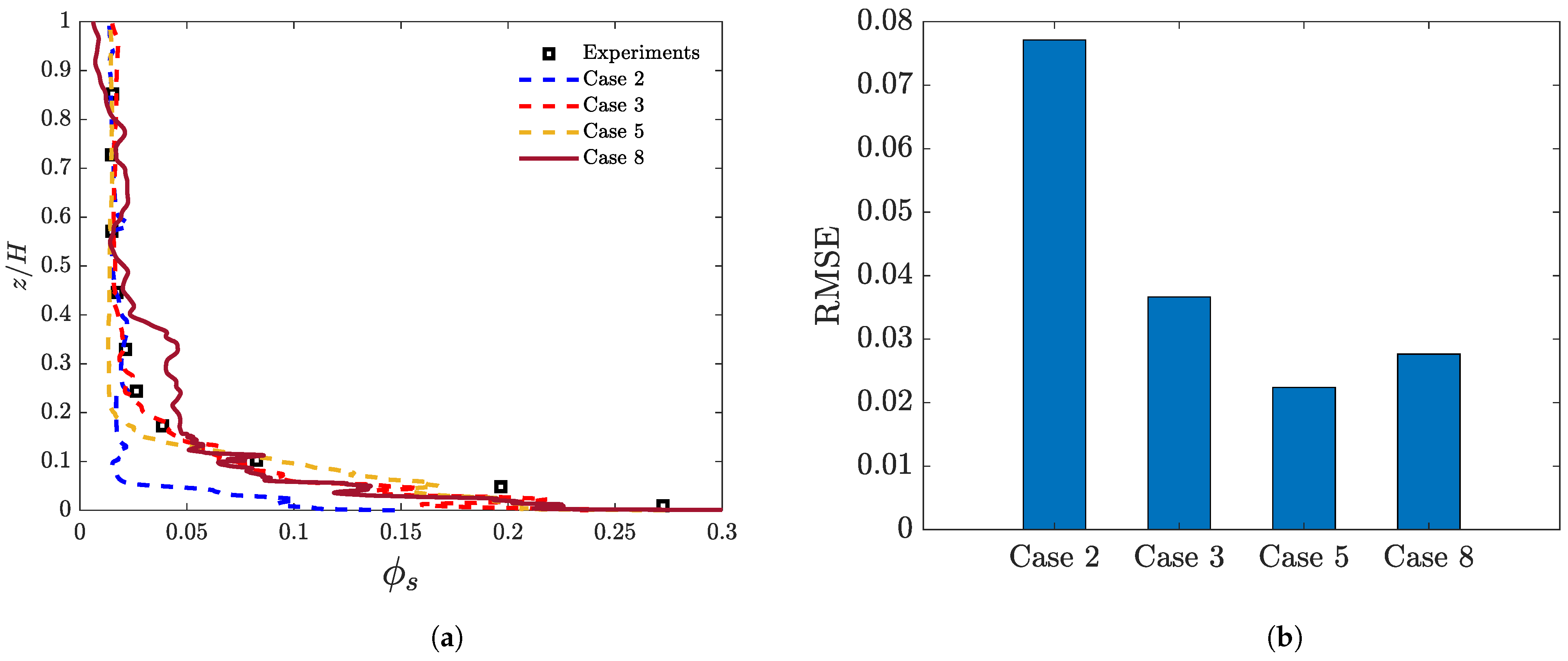
Figure 3a compares the time-averaged simulation results of solid-phase volume fraction (averaged over the cross-sectional area) and the solid holdup distribution determined from measurements of pressure drop [5] along the riser length. The experimental data exhibit an L-shape solid holdup profile along the riser height.

The challenge of accurately representing the dense bottom zone of the riser with homogeneous drag models has been reported in various numerical studies [22,40]. For example, Wang et al. [33] used Gidaspow’s drag correlation in their full-loop simulation of a CFB unit but found an underestimation of solid holdup near the bottom section of the riser. It is important to consider the effect of grid resolution on the peak value of solid volume fraction close to the gas inlet boundary (see Figure 3a). Notably, Case 5 ($2.9\times {10}^5$ cells) and Case 8 ($2.7\times {10}^6$ cells) predict nearly identical peak values for solid-phase volume fraction, making the mesh resolution of Case 5 suitable as a standard for most subsequent simulations. This choice aligns with the grid sizes used in other 3D riser simulations reported in the literature [26] and offers a more manageable computational cost compared to using a finer mesh like that employed in Case 8.

In the middle and upper dilute part of the riser, the predictions of solid volume fraction obtained from Case 5 align well with the experimental data. Utilizing a finer mesh in Case 8 does not enhance the results of solid volume fraction near the riser exit. Additionally, as previously mentioned, Case 5 required considerably less simulation time. The asymmetrical exit layout in the computational model may hinder achieving grid-independent results, especially when monitoring the axial pressure gradient (or the solid holdup), as also noted by Li et al. [26]. Overall, the RMSE values seen in Figure 3b show that the performed simulations provide predictions of solid volume fraction along the riser that are in reasonable agreement with the experimental measurements. It can be concluded that the EMMS drag model is suitable to effectively simulate the fluidization of Geldart B particles, as was also shown by Lu et al. [55] and Zhang et al. [27]. In terms of mesh sensitivity, Case 5 provides the smallest RMSE.

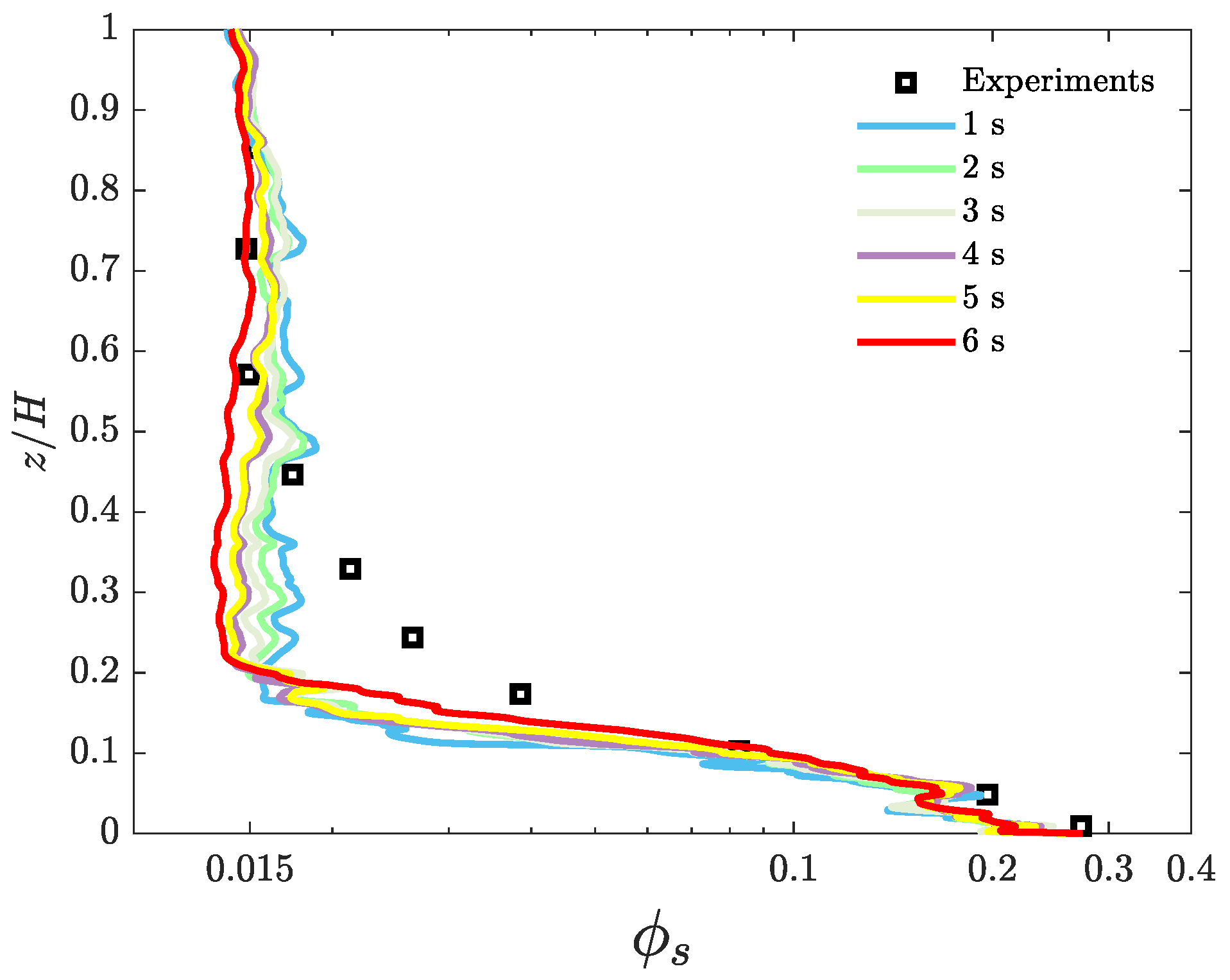
The impact of the span of time-averaging on solid holdup is illustrated in Figure 4. The results from Case 5 show that as the time-averaging period exceeds 4 s, minor discrepancies are found in the predictions of vertical solid holdup. The horizontal axis in the figure employs a logarithmic scale for better appreciation of these differences.

3.2. Two-Phase Flow in the Riser

Figure 5, Figure 6 and Figure 7 display the instantaneous time series for the solid-phase volume fraction, solid velocity, and gas velocity respectively. Contour plots depicting these variables are displayed on the central symmetry plane of the cylindrical riser at various times. These contours are obtained from Case 8 in Table 4. Furthermore, due to the riser’s substantial height-to-diameter ratio ($H/D\approx 49.4$), the figure’s height was reduced by a factor of 5 in all illustrations. This adjustment provides a clearer representation of the two-phase flow. It is worth noting that the lateral feeding elbow is not depicted.

The dynamic nature of the simulation is illustrated by these time series. Figure 5 reveals the time development of solids volume fraction in a few snapshots taken at defined times. High particle volume fraction is distinguished by the red color, while the blue color identifies very dilute regions of the two-phase flow. At 2.5 s, solids are mainly concentrated at the bottom of the riser, showing some ropes of high ${\varphi }_s$ values distributed in upper locations (up to 75% of the riser height); such ropes are quasi-horizontal in the center of the plane or vertical near the walls. The upper part of the column remains with an appreciably smaller particle volume fraction than the lower sections. At the horizontal pipe exit, the predominant color is dark blue, meaning that very few particles reach this area. At 3.0 s, an area of remarkable size of medium to low ${\varphi }_s$ (green–blue colors) is observed close to the riser bottom (below 10% of its height), which has displaced particles towards the right wall; such flow pattern is called a bubble, that is, a fluid region with a low solids volume fraction. Bubbles are identified in the contour plots as dark blue patches surrounded by intense red color areas and are typical structures of fluidized beds. Above the bubble, there is a dense area of high particle concentration, extending to approximately 20% of the riser’s height. Additionally, above this region, ropes of solids can be observed, reaching up to 50% of the riser’s height. Beyond such a point, the flow tends to be dilute, with values of ${\varphi }_s$ below 2%. At 3.5 s, the majority of the solids have descended and are located below the middle of the column, so high-concentration particle ropes are not visible in the upper half of the riser. Additionally, two areas with low solids volume fraction are identified between slugs of high values of ${\varphi }_s$ (larger than 20%) at the bottom of the cylindrical vessel. At 4.0 s, solids are mainly located at the bottom of the reactor and above a large bubble visible between 5% and 20% of the column height; such a bubble also displaces particles towards the container walls, increasing the concentration there, contributing to the annular two-phase flow regime. Finally, the snapshot at 5 s shows that the particle volume fraction is higher in the vessel bottom surrounding a large bubble that drives the solids towards the riser walls. The showcased time-series snapshots collectively unveil the dynamic evolution of high-concentration clusters and vertical streamers that continuously disappear and reform. Therefore, to compare with experimental data, it is necessary to perform a time averaging of the numerical results.

Figure 6 and Figure 7 complement the previous description of the behavior of particle volume fraction by showing snapshots, at the same time points, of solid phase (Figure 6) and gas (Figure 7) axial velocity. At 2.5 s, particles in the fluidized state have started to descend, as evidenced by the negative value of the solid-phase velocity in Figure 6; in that figure, the blue color (light and dark) indicates negative settling velocities, while the green to red colors mean positive particles rising velocity. However, gas velocities at the core of lower sections of the riser tend to be high (Figure 7) every time, coinciding with the highest solids concentration; at the exit of the riser, the contraction to the exit duct always accelerates the gas flow owing to mass conservation, which also drags some particles in this area. At 3.0 s, particle velocity in the lower 20% of the column is mainly positive, implying its fluidization in this area; however, there is a sharp axial gradient of $V_{s,z}$, meaning that the particle ropes and clusters above such region (between 20% and 60% of the column height) are settling. In the upper sections, solids show ascending velocity on the right side and settling movement on the left side. Regarding the gas velocity at 3.0 s, it is observed that a bubble region identified in this snapshot in Figure 5 presents high values in the dilute region, but it is very low near the right wall where ${\varphi }_s$ is the highest. Above the particle slug directly above the bubble, axial gas velocity is reduced in areas of higher particle concentration (the red color in Figure 5) and augmented in more dilute areas (the green to blue colors in Figure 5). Along the upper 50% length of the column, gas velocity is larger on the right side than on the left side, due to the effect of particle velocity in this area, as drag force in the fluid increases with increasing relative velocity between the phases, i.e., slip velocity.

At 3.5 s, the region of positive $V_{s,z}$ is remarkably larger and the settling velocity is lower than in the previous snapshot. Therefore, particle clusters reach higher locations in the riser. Gas velocity is again high in the dilute flow regions of the bubbles and lower in the areas with higher solids concentration surrounding them; moreover, in the upper riser sections, gas flow tends to be higher on the core than close to the walls. At 4.0 s, particles and gas axial velocity behavior are similar to that described for 3.5 s, as clusters reach similar heights on the column, although the solids ascending velocity is higher in the upper half of the riser. Particles settle down in the proximity of the left wall and in the lower region of the column where ${\varphi }_s$ is high. In the bottom sections of the vessel, gas velocity tends to increase within the bubbles and decrease in areas of high particle concentration, as mentioned before. In the upper sections, $V_{g,z}$ is greater near the right wall compared to the left wall. Finally, at 5 s, the particle velocity resembles that at 3 s, with moderate ascending velocities in the large bubble area and a sharp decrease immediately over it, where solids are settling. This zone is anticipated as one with strong inter-particle interactions owing to the high concentration and opposed velocities, positive from below and negative from above. In the upper half of the vessel, particles tend to move upwards, faster in the core than near the walls. Regarding the gas velocity, it is the highest in the core of lower riser sections due to the bubble presence. In the upper cylinder region, the gas rises faster near the core than the walls, showing a similar behavior to $V_{s,z}$.

In summary, the two-phase flow within the CFB riser displays complex dynamics involving a variety of physical phenomena whose modeling is really challenging and still in development.

Figure 8a shows the comparison of the solid-phase radial distribution obtained from Case 8 with experimental data. The corresponding RMSE values at each elevation are depicted in Figure 8b. It is clear that the simulations effectively capture the decreasing solid volume fraction as riser height increases. The deviation between experimental data and simulation results from Case 8 decreases in the axial direction. Furthermore, the peak ${\varphi }_s$ near the walls is qualitatively well captured, especially for the lower sections. In contrast, in higher sections, simulation profiles are slightly flatter than their experimental counterparts, though a slight increase in particles near the walls is still noticeable. Overall, there is an acceptable agreement between the experiments and computations, which is anticipated to improve with increased average time on this fine grid case. However, conducting extended simulations on a finer grid poses an excessive computational burden not feasible with the currently available hardware.

3.3. Effects of Drag Model and Turbulence Modulation on Solid Distribution in the Riser

Figure 9 illustrates the comparison of time-averaged axial (Figure 9a) and radial profiles (Figure 9b–d) of the solid-phase volume fraction in selected vertical cross-sections. In the case of 3D simulations (Cases 4 to 9), the profiles are extracted at the center plane ($y=0$, as depicted in Figure 2a). These profiles were derived from simulations employing three drag models (Cases 4, 5, and 6), the omission of turbulence modulation terms (Case 7), and the utilization of a different turbulence model (Case 9 uses k-$ϵ$ model). Results from a simplified two-dimensional domain (Case 1) are also included for completeness.

Comparing the 2D and 3D computational domains, the simulation results show that for both domains, the solid-phase volume fraction decreases with height, following the experimental trend, as is seen in Figure 9a. However, in the 2D domain, the vertical profile values of ${\varphi }_s$ are above those of the 3D domain in the bottom part of the riser but present lower values in the upper zone. This fact is corroborated by graphs in Figure 9b–d. In fact, a 2D approximation overestimates fluidization of solid particles in the lower zone and under-predicts it in the upper part compared to a full 3D representation, being insufficient to adequately describe particle distribution. This behavior might be due to substantial interparticle interactions imposed within a two-dimensional domain. Conversely, in a 3D environment, particle trajectories unfold within a volume, diminishing the likelihood of direct interaction between particles.

Cases 5 and 9 illustrate the sensitivity of the computations to the modeling of the turbulent dynamics of the flow while remaining within the frame of two-equation turbulence models. These considerations are significant in understanding how different turbulence models affect computational results, particularly when comparing between k-$\omega$ SST and standard k-$ϵ$ model evaluations. From Figure 9, it is clear that in Case 9, the ${\varphi }_s$ values at the bottom of the riser exceed those in Case 5 (see Figure 9b), resulting in an overestimation of the experimental measurements. However, in the uppermost sections (Figure 9c,d), the ${\varphi }_s$ profiles in Case 9 exhibit lower values compared to Case 5, indicating flatter profiles and a loss of their core–annular shape with volume fraction peaks near the wall. This behavior suggests that the deficiencies inherent in the k-$ϵ$ model near walls lead to these flat profiles. It further implies that the k-$\omega$ SST model offers a more accurate depiction of the gas–solid flow near walls compared to the standard k-$ϵ$ approach.

The preceding explanation is supported by RMSE calculations for radial profiles at three analyzed elevations, as shown in Figure 10. Case 9 displays a larger RMSE at the topmost elevations, while some discrepancies are found between Cases 5 and 8 at the riser wall in these upper sections. These differences can be explained by variations in mesh resolution and time-averaging window. The radial profile obtained with the fine mesh (Case 8) at $z/H=0.048$ shows the best agreement with the experimental data, holding the lowest RMSE. This result suggests that a sufficiently fine grid resolution is needed to capture the dynamics of the riser’s dense bottom section.

Disregarding two-way coupling, i.e., ignoring the interaction terms (Equations (2) and (3)) in the turbulent variables equations, is considered in Case 7. Nearly uniform solid-phase volume fraction profiles are found in the upper section of the riser when turbulence modulation terms are omitted, contrary to the core–annular distribution suggested by the experimental data. It is also noteworthy that Case 7 and Case 9 (k-$ϵ$ turbulence model) have nearly the same RMSE value at the highest elevations. In the bottom section of the riser, the ${\varphi }_s$ curve obtained in Case 7 tends to be higher than the measurements and the profiles obtained in Cases 5 and 8. These observations reflect the importance of considering two-way coupling in the numerical simulations of CFB risers and show the insufficiency of some previously documented numerical studies in this kind of systems [22,26,41,56].

The Wen and Yu and Syamlal–O’Brien drag correlations fail to capture the dense bottom bed observed in the experiments. Cases 4 and 6 exhibit the largest RMSE for the radial profiles at the riser bottom section. In this respect, simulations incorporating the EMMS drag model show a significant improvement in reproducing the dense bottom section and a more dilute region towards the top of the riser, as clearly illustrated in Figure 9a, following the trend depicted by the experiments.

Cases 5 and 8 successfully replicate the highest solid volume fraction seen in CFB experiments, consistent with the previous studies using the EMMS drag model in a 2D domain [23]. Interestingly, when comparing results in the upper sections of the CFD riser, the computation of drag force using the Syamlal–O’Brien correlation produces a more distinct core–annular solid distribution (Figure 9c,d) compared to Case 4 and implementation of the EMMS drag model (Cases 5 and 8). In fact, in the topmost sections, Wen and Yu and EMMS (Case 8) models offer similar profiles, although Case 4 tends to be more symmetrical. Cases 4 and 8 fail to accurately reproduce near-wall peaks at $z/H=0.64$. Regarding RMSE values, Cases 4 and 6 show similar performances with the lowest value in the top section.

From the simulated radial profiles of solid volume fraction, it can be concluded that the Wen and Yu and Syamlal–O’Brien drag models perform much better in the dilute regime. However, when evaluating the performance of these different drag models, only the EMMS drag model reproduces the trend of the experimental measurements along the entire riser height in both the axial and radial directions.

4. Conclusions

In this work, a computational study of the turbulent gas–solid flow in a cold-CFB riser is conducted using an E-E approach (the two-fluid model) that incorporates closures from the kinetic theory of granular flow and two-equation turbulence models along with turbulence modulation terms. The effect of three drag model correlations, namely, Wen and Yu, Syamlal–O’Brien, and EMMS models, on the axial and radial profiles of the solid phase in the riser is investigated. Calculations of a turbulent gas–solid flow in a simplified 2D computational model of the riser are also compared with the set of simulations performed in a 3D domain. The main conclusions of the study are the following:

• The investigation into three drag model correlations (Wen and Yu, Syamlal–O’Brien, and EMMS models) revealed notable variations in the axial and radial profiles of the solid-phase concentration along the riser height. The differences were quantified in terms of the root mean square error (RMSE).
• The EMMS drag model emerged as the most effective in reproducing both the axial and radial measured profiles of solid volume fraction, particularly at the bottom of the riser, where other models failed. This fact illustrates the critical role of drag model selection in providing an adequate prediction of the peak solid volume fraction, emphasizing the superiority of the EMMS model in agreement with the experimental data.
• A mesh sensitivity analysis underscored the importance of finely adjusted mesh resolution for reliable results in riser simulations. The time-averaging window also needs to be sufficiently long.
• The comparison between the 2D and 3D computational models of the riser with experiments pointed out the insufficiency of two-dimensional computations due to an overestimation of particle–particle interactions. Such a mechanism leads to an excessive spreading of solids in the upper cross-sections, not reflecting the measured annular core shape of particle distribution.
• The predictions of radial solid distribution in the riser were also found to be influenced by the choice of turbulence model, turbulence modulation, and computational domain configuration. In particular, neglecting the turbulence modulation terms leads to a nearly uniform distribution of particles in the upper riser sections, failing to reproduce the observed annular core shape.

A limitation of the performed study has been the consideration of a single particle size; the future research will be focused on exploring the impact of using a particle size distribution and varying solid wall boundary conditions on the axial and radial solid volume fraction profiles.