An Efficient Numerical Method for Solving a Class of Nonlinear Fractional Differential Equations and Error Estimates

Abstract

In this paper, we present an efficient method for solving a class of higher order fractional differential equations with general boundary conditions. The convergence of the numerical method is proved and an error estimate is given. Finally, eight numerical examples, both linear and nonlinear, are presented to demonstrate the accuracy of our method. The proposed method introduces suitable base functions to calculate the approximate solutions and only requires us to deal with the linear or nonlinear systems. Thus, our method is convenient to implement. Furthermore, the numerical results show that the proposed method performs better compared to the existing ones.

1. Introduction

The study of nonlinear fractional differential equations has attracted a lot of attention in recent years due to their widespread applications in the natural sciences. The history of fractional differential equations can be traced back to three hundred years ago. Leibniz and Euler first studied such equations. Then L’Hospital, Laplace, and Caputo made great contributions to fractional differential equation theory. In recent years, more and more researchers have devoted themselves to working on such equations. The application and theory of fractional equations are developing rapidly. The reader may refer to [1,2,3,4,5] for recent developments in fractional differential equations.

In this paper, we study the numerical method for solving nonlinear fractional BVPs:

$$\begin{array}{cc}\hfill & p_0\left(x\right)u^{\left({\alpha }_0\right)}\left(x\right)+p_1\left(x\right)u^{\left({\alpha }_1\right)}\left(x\right)+\cdots +p_{m-1}\left(x\right)u^{\left({\alpha }_{m-1}\right)}\left(x\right)+p_m\left(x\right)u^{\left({\alpha }_m\right)}\left(x\right)=f(x,u),\hfill \\ \hfill & {\lambda }_{i}u=r_i,(i=1,2,...,N),\hfill \end{array}$$

(1)

where $0\le x\le 1$, $m_j-1<{\alpha }_j<m_j$, $m_j$ is a positive integer, $m=max\left\{m_j\right\}$. $p_j\left(x\right)\in L^2[0,1]$, $(j=0,1,2,...,m)$. ${\lambda }_{i}u(i=1,2,...,N)$ are boundary conditions. If ${\lambda }_{i}u={\int }_0^1{k}_i\left(t\right)u\left(t\right)dt(i=1,2,...,N)$, problem (1) is a nonlocal problem. If ${\lambda }_{i}u=u\left(x_i\right)(i=1,2,...,N)$, problem (1) is a multi-point problem, and so on. The $\alpha$-order Caputo derivative of $u\left(x\right)$ is defined in Definition 1.

Definition 1. 

The Caputo fractional derivative of order $\alpha >0$ is defined as

$$D^{\alpha }u\left(x\right)=\frac{1}{\Gamma (N-\alpha )}{\int }_0^x{(x-t)}^{N-\alpha -1}{u}^{\left(N\right)}\left(t\right)dt$$

(2)

 where $0<x<1$, $N-1<\alpha <N$, and $N\in \mathbb{N}$.

Based on Definition 1, the problem is equivalent to the following problem:

$$\begin{array}{cc}\hfill & Lu\triangleq \sum _{j=0}^m\frac{p_j\left(x\right)}{\Gamma (m_j-{\alpha }_j)}{\int }_0^x{(x-t)}^{m_j-{\alpha }_j-1}{u}^{\left(m_j\right)}\left(t\right)dt=f(x,u),x\in [0,1],\hfill \\ \hfill & {\lambda }_{i}u=r_i,(i=1,2,...,N),\hfill \end{array}$$

(3)

where $m_j-1<{\alpha }_j<m_j$, $m=max\left\{m_j\right\}$. Over the last couple of years, many numerical methods [6,7,8,9,10,11,12,13,14,15,16,17,18] have been developed for solving problem (3). However, the accuracy of the above method cannot meet our requirements. In this paper, we introduce polynomial base functions to solve (3). The proposed method only requires dealing with a nonlinear system; thus, it is easy to implement. Furthermore, the proposed method is more accurate than the other numerical methods.

This paper is organized as follows. In Section 2, we propose the method for solving problem (3). Then, we analyze the convergence and give an error estimate in Section 3. In Section 4, we present eight numerical examples to show the accuracy of the method. Finally, the conclusions are drawn in Section 6.

2. Numerical Method

Now, we will examine the method for solving problem (3). Considering the function space whose base functions are

$$\mathbf{X}=[{\phi }_0\left(x\right),{\phi }_1\left(x\right),{\phi }_2\left(x\right),{\phi }_3\left(x\right),\dots ],$$

then, the true solution of (3) can be given by

$$u\left(x\right)=\sum _{k=0}^{\infty }{\beta }_k{\phi }_k\left(x\right),$$

(4)

where ${\beta }_k$ is to be determined.

Let

$${\mathbf{X}}_n=[{\phi }_0\left(x\right),{\phi }_1\left(x\right),{\phi }_2\left(x\right),\dots ,{\phi }_n\left(x\right)],$$

and

$${\mathbf{Y}}_n={[{\beta }_0,{\beta }_1,{\beta }_2,\dots ,{\beta }_n]}^T,$$

then, the n-th order approximate solution of (3) can be expressed by

$$u_n\left(x\right)=\sum _{k=0}^n{\beta }_k{\phi }_k\left(x\right)={\mathbf{X}}_n{\mathbf{Y}}_n.$$

(5)

Furthermore, the higher derivatives of $u_n\left(x\right)$ can also be calculated by

$$u_n^{\left(i\right)}={\mathbf{X}}_n{\mathbf{B}}^i{\mathbf{Y}}_n,i\ge 1,$$

(6)

where matrix $\mathbf{B}$ is dependent on the choice of ${\mathbf{X}}_n$.

Assuming $H=L^2[a,b]$ is the working space with inner product,

$$<f,g>={\int }_a^{b}f\left(x\right)g\left(x\right)dx.$$

Substituting Equation (6) into (3), we have

$$L{u}_n=f(x,u_n).$$

(7)

Assume that $\mathbf{Q}=[{\psi }_0\left(x\right),{\psi }_1\left(x\right),{\psi }_2\left(x\right),\dots ,{\psi }_n\left(x\right)]$ is a linear independent set in H. Taking the inner product of Equation (7) with the element in $\mathbf{Q}$, two new matrices ${\mathbf{S}}_{(n+1)\times 1}$ and ${\mathbf{T}}_{(n+1)\times 1}$ are defined as

$${\mathbf{S}}_{(n+1)\times 1}={\mathbf{T}}_{(n+1)\times 1},$$

and

$${\mathbf{S}}_{q,1}=<L{u}_n,{\psi }_{q-1}>,$$

$${\mathbf{T}}_{q,1}=<f(x,u_n),{\psi }_{q-1}\left(x\right)>,$$

where $1\le q\le n+1$.

Considering the boundary conditions in problem (3),

$${\lambda }_i{u}_n=r_i,(i=1,2,...,N),$$

(8)

these N equations just modify N rows of ${\mathbf{S}}_{(n+1)\times 1}$ and ${\mathbf{T}}_{(n+1)\times 1}$, respectively. If the linear or nonlinear system $\mathbf{S}=\mathbf{T}$ is solved, the coefficients ${\mathbf{Y}}_n={[{\beta }_0,{\beta }_1,{\beta }_2,\dots ,{\beta }_n]}^T$ are determined uniquely. Then, the numerical solution of (3) can be expressed by

$$u_n\left(x\right)=\sum _{k=0}^n{\beta }_k{\phi }_k\left(x\right).$$

(9)

Notice that continuous polynomials $\{x^k:k\in \mathbb{Z}\}$ are recommended when ${\mathbf{X}}_n$ is chosen since they are calculated rapidly, precisely defined, and can represent a variety of functions [19].

3. The Convergence of the Method and Error Estimate

Suppose that $H=L^2[a,b]$ is the working space, $P_n=\{{\varphi }_0,{\varphi }_1,\cdots ,{\varphi }_n\}$ is the set of polynomials of n-th degree and $Y=span\left(P_n\right)$. Then, the $L_2$-error can be achieved [19,20]. For $\forall u\in H$, u has the unique best approximation in Y. That is to say that there exists $\overline{u}\in Y$, such that

$$\parallel u-\overline{u}{\parallel }_2\le {\parallel u-h\parallel }_2,for\forall h\in Y.$$

Let $\Phi ={[{\varphi }_0,{\varphi }_1,\cdots ,{\varphi }_n]}^T$; there exists unique coefficients $\mathbf{A}=[a_0,a_1,\cdots ,a_n]$ such that

$$u\simeq \overline{u}=\sum _{i=0}^n{a}_i{\varphi }_i=\mathbf{A}\Phi ,$$

$\mathbf{A}$ can be obtained by

$$\mathbf{A}<\Phi ,\Phi >=<u,\Phi >,$$

where

$$<u,\Phi >={\int }_a^{b}y\left(x\right)\Phi {\left(x\right)}^{T}dx=[<u,{\varphi }_0>,<u,{\varphi }_1>,\cdots ,<u,{\varphi }_n>],$$

and $<\Phi ,\Phi >$ is a $(n+1)\times (n+1)$ matrix. Let

$$\mathbf{C}=<\Phi ,\Phi >={\int }_a^b\Phi \left(x\right)\Phi {\left(x\right)}^{T}dx,$$

then,

$$\mathbf{A}=<u,\Phi >{\mathbf{C}}^{-1}.$$

Since the coefficients $\mathbf{A}$ are determined, we obtain the approximate solution $\overline{u}$. We have the following conclusion. Since we have defined the inner product in H by $<f,g>={\int }_a^{b}f\left(x\right)g\left(x\right)dx$ and $Y=span\left(P_n\right)$, then $L_2$-error can be obtained by

$$\parallel u-\overline{u}{\parallel }_2^2=\frac{det[{\int }_a^b\Psi \left(x\right)\Psi {\left(x\right)}^{T}dx]}{det[{\int }_a^b\Phi \left(x\right)\Phi {\left(x\right)}^{T}dx]},$$

where $\Phi ={[{\varphi }_0,{\varphi }_1,\cdots ,{\varphi }_n]}^T$ and $\Psi ={[y,{\varphi }_0,{\varphi }_1,\cdots ,{\varphi }_n]}^T$.

Next, we will prove that the approximation $\overline{u}$ converges to u.

Lemma 1. 

A function $u\left(x\right)$ is continuous on $[a,b]$ if and only if

$$\underset{\delta \to 0}{lim}\omega (u,\delta )=0,$$

 $\omega (u,\delta )=sup|u\left(x_1\right)-u\left(x_2\right)|$ where $x_1,x_2\in [a,b]and|x_1-x_2|\le \delta$.

Proof. 

Refer to [21].    □

If $u\left(x\right)$ is bounded on $[a,b]$, we come to the following conclusion.

Lemma 2. 

If $u\left(x\right)$ is bounded on $[a,b]$, then

$${∥u-\sum _{k=0}^{n}u\left(\frac{k}{n}\right){\varphi }_k∥}_{\infty }\le \frac{3}{2}\omega \left(u,\sqrt{\frac{1}{n}}\right),$$

 where ${\parallel f\left(x\right)\parallel }_{\infty }=sup\left\{\right|f\left(x\right)|:x\in [a,b]\}$.

Proof. 

Refer to [21].    □

Theorem 1. 

If $u\left(x\right)$ is bounded on interval $[a,b]$ and $Y=span\left\{P_n\right\}$, then

$${\parallel u-\mathbf{A}\Phi \parallel }_2\le \frac{3}{2}\omega \left(u,\sqrt{\frac{1}{n}}\right),$$

(10)

 where $\mathbf{A}\Phi$ is the best approximation to u in Y.

Proof. 

Since $\mathbf{A}\Phi$ is the best approximation to u in Y, then

$${\parallel u-\mathbf{A}\Phi \parallel }_2\le {∥u-\sum _{k=0}^{n}u\left(\frac{k}{n}\right){\varphi }_k∥}_2\le {∥u-\sum _{k=0}^{n}u\left(\frac{k}{n}\right){\varphi }_k∥}_{\infty }\le \frac{3}{2}\omega \left(u,\sqrt{\frac{1}{n}}\right).$$

□

If $u\left(x\right)$ is continuous on $[a,b]$, then we have the following conclusion by Lemma 1

$$\underset{n\to \infty }{lim}\omega \left(u,\sqrt{\frac{1}{n}}\right)=0,$$

which means that $\mathbf{A}\Phi$ converges to u when $n\to \infty$.

If u is $n+1$ times continuously differentiable, the following conclusion can be obtained.

Theorem 2. 

Suppose $u\left(x\right)$ is the true solution and $u_n\left(x\right)$ is the approximate solution to problem (3), $Y=span\left(P_n\right)$ and $u_n$ is the best approximation to u in Y, $u\in C^{n+1}[a,b]$, an $L_2$-error estimate is given by

$$\parallel u-u_n{\parallel }_2\le \frac{M{(b-a)}^{\frac{2n+3}{2}}}{\sqrt{2n+3}·(n+1)!},$$

(11)

 where $M=\underset{x\in [a,b]}{max}\left|u^{(n+1)}\left(x\right)\right|$.

Proof. 

Using Taylor’s formula,

$$u_n\left(x\right)=u\left(a\right)+u^{\prime }\left(a\right)(x-a)+\frac{u^{″}\left(a\right)}{2!}{(x-a)}^2+\cdots +\frac{u^{\left(n\right)}\left(a\right)}{n!}{(x-a)}^n+R_n\left(x\right),$$

where $R_n\left(x\right)=\frac{u^{(n+1)}\left(\eta \right)}{(n+1)!}{(x-a)}^{n+1}$, $\eta \in (a,b)$. And let

$$p\left(x\right)=u\left(a\right)+u^{\prime }\left(a\right)(x-a)+\frac{u^{″}\left(a\right)}{2!}{(x-a)}^2+\cdots +\frac{u^{\left(n\right)}\left(a\right)}{n!}{(x-a)}^n.$$

Then, we have

$$\begin{array}{cc}\hfill \parallel u-u_n{\parallel }_2& \le {\parallel u-p\parallel }_2\le \sqrt{{\int }_a^b{|y\left(x\right)-p\left(x\right)|}^{2}dx}\le \sqrt{{\int }_a^b{R}_n^2\left(x\right)dx}\hfill \\ \hfill & \le \frac{M{(b-a)}^{\frac{2n+3}{2}}}{\sqrt{2n+3}·(n+1)!},\hfill \end{array}$$

where $M=\underset{x\in [a,b]}{max}\left|u^{(n+1)}\left(x\right)\right|$.    □

4. Applications of the Method

In this section, eight numerical examples are presented to demonstrate the accuracy of the proposed method.

Example 1. 

Consider the following Bagley–Torivik equation [22]:

$$\begin{array}{cc}\hfill & [D^2+D^{3/2}+D^0]u\left(x\right)=2+x^2+\frac{4\sqrt{x}}{\sqrt{\pi }},x\in [0,1],\hfill \\ \hfill & u\left(0\right)=0,u^{\prime }\left(0\right)=0.\hfill \end{array}$$

(12)

The exact solution is $u\left(x\right)=x^2$. Our results are shown in Equation (13). The exact solution can be obtained by our method. The numerical result is shown in Figure 1.

$$\begin{array}{cc}\hfill & u_0\left(x\right)=0,\hfill \\ \hfill & u_1\left(x\right)=0,\hfill \\ \hfill & u_n\left(x\right)=x^2,n\ge 2.\hfill \end{array}$$

(13)

Example 2. 

Consider the following fractional differential equation [23]:

$$\begin{array}{cc}\hfill & D^{1/2}u\left(x\right)+\sqrt{\pi }u\left(x\right)=\frac{8}{3\sqrt{\pi }}+\sqrt{\pi }{x}^2,x\in [0,1],\hfill \\ \hfill & u\left(0\right)=0.\hfill \end{array}$$

(14)

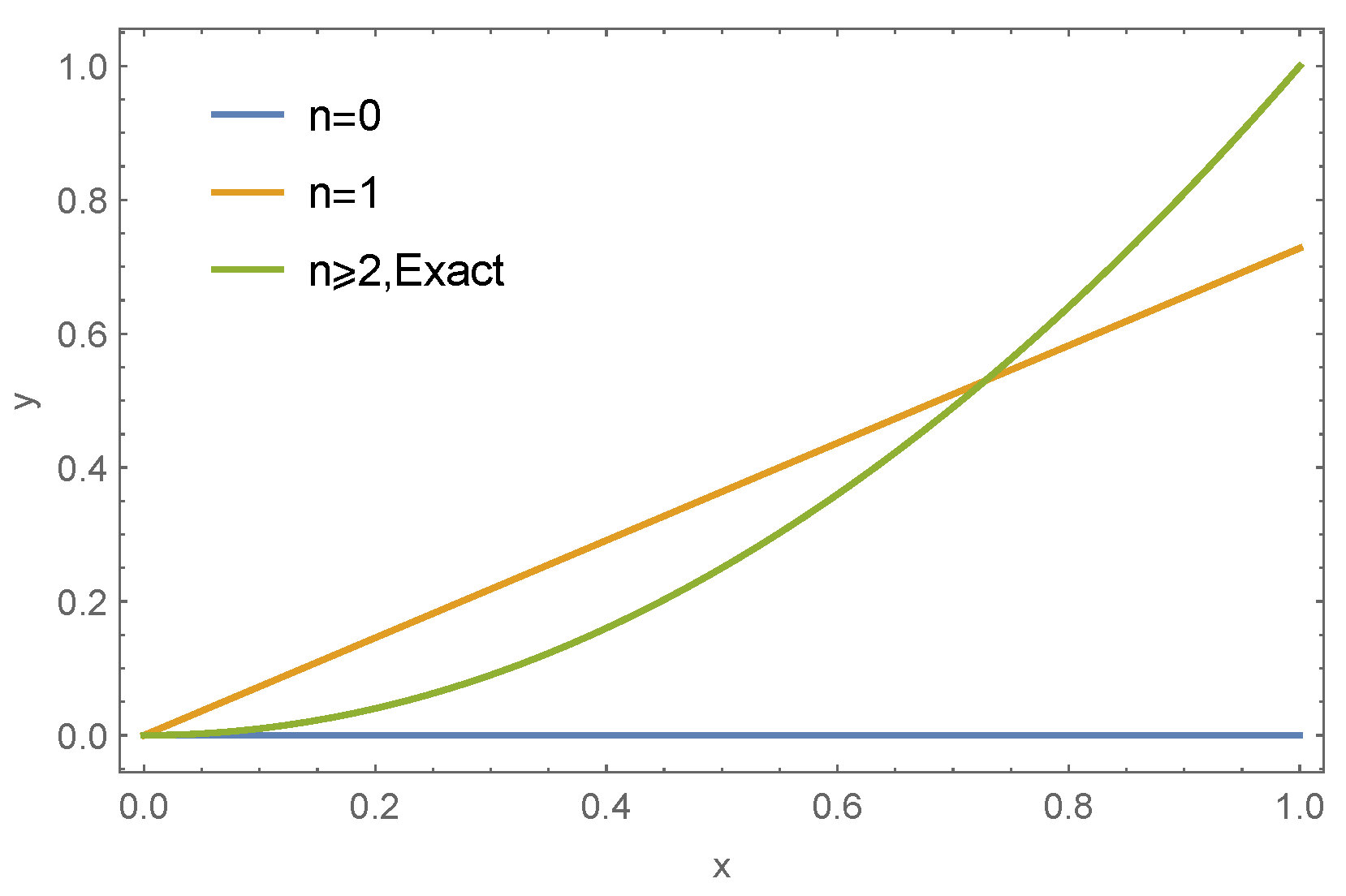
The exact solution is $u\left(x\right)=x^2$. The results are shown in Equation (15). The true solution is achieved by the proposed method. The numerical result is presented in Figure 2.

$$\begin{array}{cc}\hfill & u_0\left(x\right)=0,\hfill \\ \hfill & u_1\left(x\right)=\frac{32+10\pi }{40+15\pi }x,\hfill \\ \hfill & u_n\left(x\right)=x^2,n\ge 2.\hfill \end{array}$$

(15)

Example 3. 

Let us consider the following fractional differential equation [23]:

$$\begin{array}{cc}\hfill & [D^{1/4}+D^0]u\left(x\right)=-\frac{x^3}{2}+x^4+\frac{64x^{11/4}(32x-15)}{1155\Gamma \left(\frac{3}{4}\right)},\hfill \\ \hfill & u\left(0\right)=0.\hfill \end{array}$$

(16)

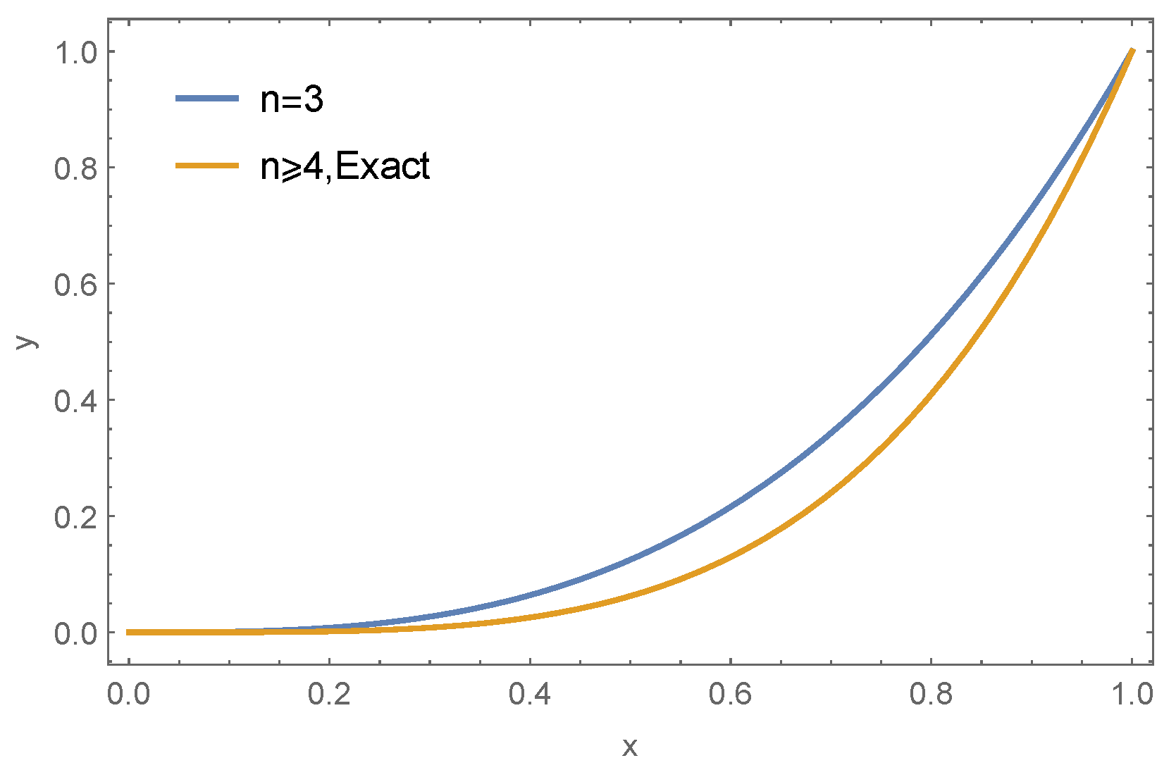
The exact solution is $u\left(x\right)=x^4-\frac{x^3}{2}$. Our solutions for various n are shown in Equation (17). The plots of the numerical solutions and the exact solution are shown in Figure 3. It can be found that the numerical solutions converge to the exact solution quickly.

$$\begin{array}{cc}\hfill & u_0\left(x\right)=0,\hfill \\ \hfill & u_1\left(x\right)=\frac{-26624-13167c}{4180(32+21c)}x,\hfill \\ \hfill & u_2\left(x\right)=\frac{-687865856-728437248c-194322975c^2}{8740(262144+303072c+88935c^2)}x+\frac{3(26214400+28519568c+7772919c^2)}{437(262144+303072c+88935c^2)}{x}^2,\hfill \\ \hfill & u_3\left(x\right)=\frac{4(140737488355328+215214653964288c+110716498835712c^2+19167948297729c^3)}{3933(1099511627776+1753074892800c+941834456640c^2+170576707455c^3)}x\hfill \\ \hfill & -\frac{2(35184372088832+54747587411968c+28650322067136c^2+5044196920455c^3)}{69(1099511627776+1753074892800c+941834456640c^2+170576707455c^3)}{x}^2\hfill \\ \hfill & +\frac{-25288767438848-39712678477824c-20978221978560c^2-3728319462945c^3}{18(1099511627776+1753074892800c+941834456640c^2+170576707455c^3)}{x}^3,\hfill \\ \hfill & u_n\left(x\right)=-\frac{1}{2}{x}^3+x^4,n\ge 4,\hfill \end{array}$$

(17)

 where $c=\Gamma \left(\frac{3}{4}\right)$. Again, the true solution is obtained by the proposed method.

Example 4. 

Now consider the following Liouville–Bratu–Gelfand equation [6,14,24,25]:

$$\begin{array}{cc}\hfill & u^{″}\left(x\right)+\lambda e^{u\left(x\right)}=0,\hfill \\ \hfill & u\left(0\right)=0,u\left(1\right)=0.\hfill \end{array}$$

(18)

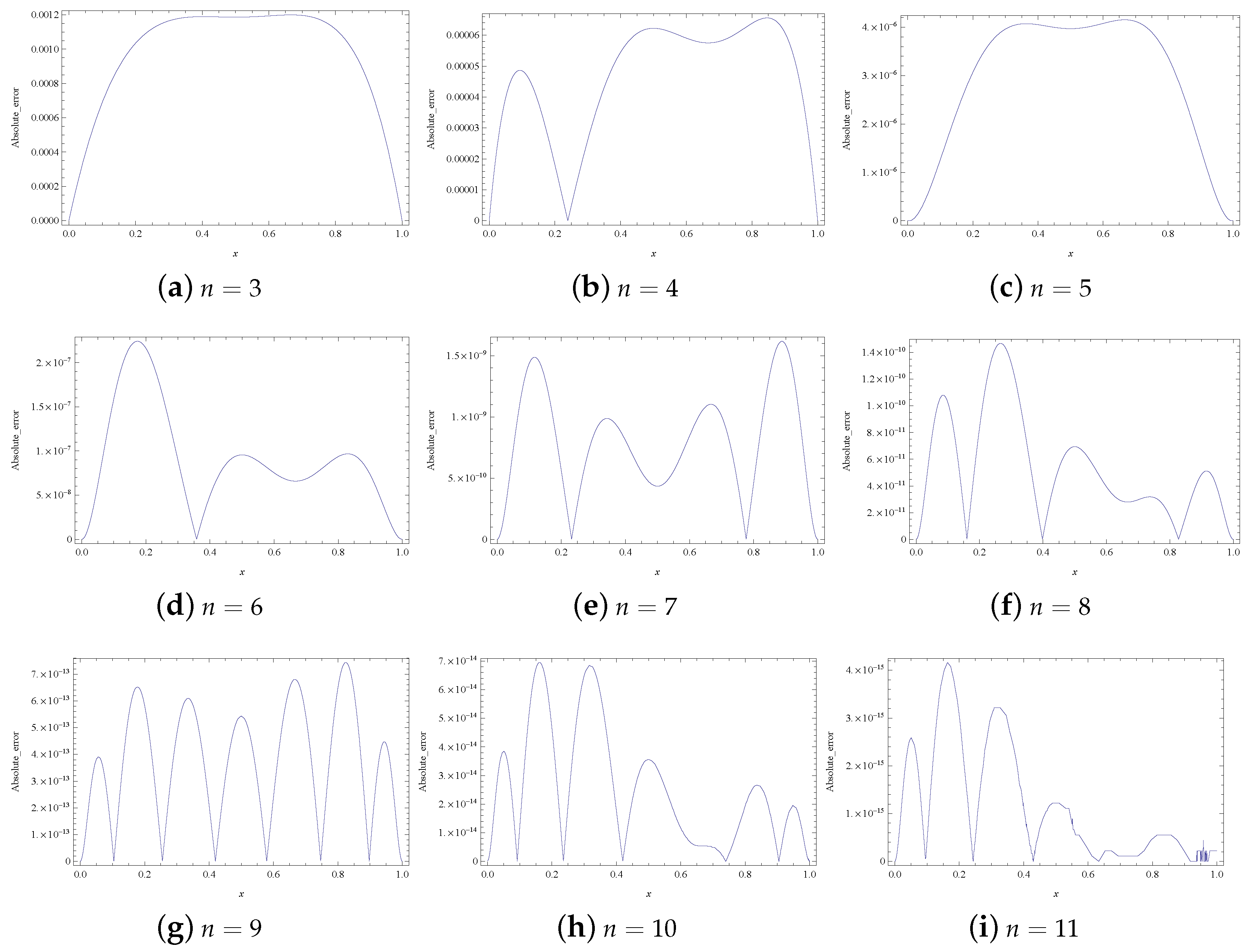
The exact solution is $u\left(x\right)=-2ln\left[\frac{cosh\left((x-\frac{1}{2})\frac{\theta }{2}\right)}{cosh\left(\frac{\theta }{4}\right)}\right]$, where θ is the solution of $\theta =\sqrt{2\lambda }cosh\left(\frac{\theta }{4}\right)$. The absolute errors when $n=10$ are shown in

Table 1. Comparison of absolute errors for Example 4.

$\mathit{\lambda }$	Node	LGSM [6]	B-spline [7]	Laplace [8]	ADM [9]	RKSM [23]	Present Method
	0.1	7.5 $\times {10}^{-7}$	3.0 $\times {10}^{-6}$	2.0 $\times {10}^{-6}$	2.7 $\times {10}^{-3}$	6.2 $\times {10}^{-5}$	2.8 $\times {10}^{-10}$
	0.2	1.0 $\times {10}^{-6}$	5.5 $\times {10}^{-6}$	3.9 $\times {10}^{-6}$	2.0 $\times {10}^{-3}$	1.1 $\times {10}^{-4}$	3.6 $\times {10}^{-10}$
$\lambda =1$	0.4	5.2 $\times {10}^{-7}$	8.5 $\times {10}^{-6}$	7.7 $\times {10}^{-6}$	2.2 $\times {10}^{-3}$	1.7 $\times {10}^{-4}$	2.5 $\times {10}^{-10}$
	0.6	5.1 $\times {10}^{-7}$	8.5 $\times {10}^{-6}$	1.1 $\times {10}^{-5}$	2.2 $\times {10}^{-3}$	1.6 $\times {10}^{-4}$	2.5 $\times {10}^{-10}$
	0.9	7.4 $\times {10}^{-7}$	3.0 $\times {10}^{-6}$	1.2 $\times {10}^{-5}$	2.7 $\times {10}^{-3}$	5.6 $\times {10}^{-5}$	2.8 $\times {10}^{-10}$
	0.2	5.7 $\times {10}^{-6}$	1.9 $\times {10}^{-5}$	4.2 $\times {10}^{-3}$	1.5 $\times {10}^{-2}$	5.8 $\times {10}^{-4}$	5.0 $\times {10}^{-8}$
	0.3	5.2 $\times {10}^{-6}$	2.8 $\times {10}^{-5}$	6.2 $\times {10}^{-3}$	5.9 $\times {10}^{-3}$	7.9 $\times {10}^{-4}$	2.0 $\times {10}^{-8}$
$\lambda =2$	0.5	1.5 $\times {10}^{-6}$	1.1 $\times {10}^{-5}$	9.6 $\times {10}^{-3}$	7.0 $\times {10}^{-3}$	9.7 $\times {10}^{-4}$	6.6 $\times {10}^{-8}$
	0.7	5.2 $\times {10}^{-6}$	6.9 $\times {10}^{-5}$	1.2 $\times {10}^{-2}$	5.9 $\times {10}^{-3}$	7.8 $\times {10}^{-4}$	2.0 $\times {10}^{-8}$
	0.9	4.0 $\times {10}^{-6}$	2.6 $\times {10}^{-5}$	1.1 $\times {10}^{-2}$	1.5 $\times {10}^{-2}$	3.0 $\times {10}^{-4}$	4.4 $\times {10}^{-8}$

. It can be found that our method performs better than the other methods. The curves of the absolute errors are plotted in Figure 4 and Figure 5 for $\lambda =1$ and $\lambda =2$ respectively.

Example 5. 

Consider the following nonlinear boundary value problem [13,26,27,28,29]:

$$\begin{array}{cc}\hfill & u^{\left(5\right)}\left(x\right)=e^{-x}{u}^2\left(x\right),\hfill \\ \hfill & u\left(0\right)=u^{\prime }\left(0\right)=u^{″}\left(0\right)=1,u\left(1\right)=u^{\prime }\left(1\right)=e.\hfill \end{array}$$

(19)

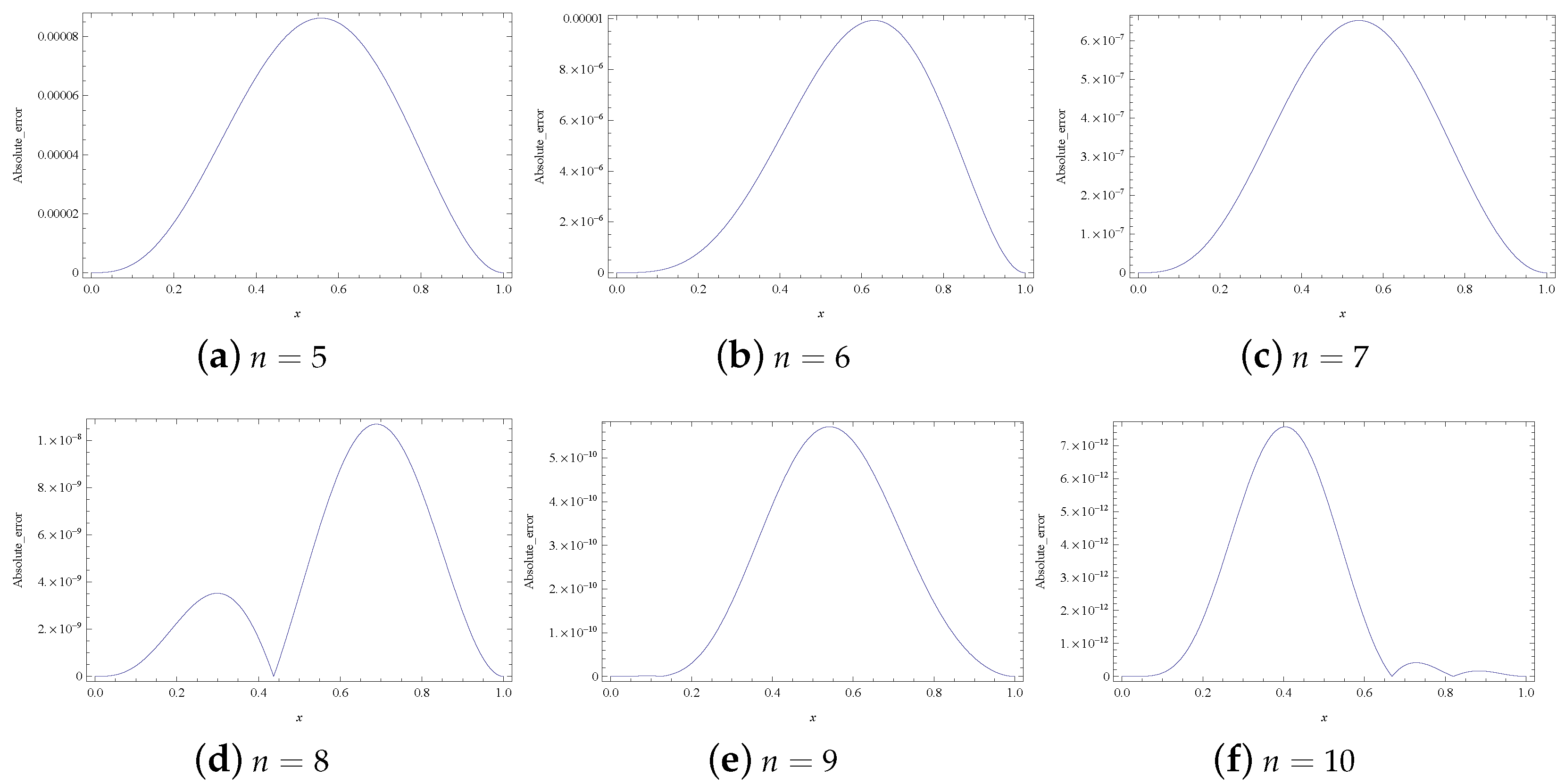
The exact solution is $u\left(x\right)=e^x$. Our result when $n=10$ is shown in Equation (20). The comparison with the other methods is shown in

Table 2. Comparison of absolute errors for Example 5.

Node	ADM [10]	HPM [11]	VIMHP [11]	VIM [11]	B-Spline [12]	Method in [13]	Method in [14]	RKSM [23]	Present Method
0.1	1.0 $\times {10}^{-9}$	1.0 $\times {10}^{-9}$	1.0 $\times {10}^{-9}$	1.0 $\times {10}^{-9}$	7.0 $\times {10}^{-4}$	2.3 $\times {10}^{-7}$	0	7.1 $\times {10}^{-10}$	1.1 $\times {10}^{-13}$
0.2	2.0 $\times {10}^{-9}$	2.0 $\times {10}^{-9}$	2.0 $\times {10}^{-9}$	2.0 $\times {10}^{-9}$	7.2 $\times {10}^{-4}$	1.6 $\times {10}^{-6}$	1.0 $\times {10}^{-5}$	4.6 $\times {10}^{-9}$	1.7 $\times {10}^{-12}$
0.3	1.0 $\times {10}^{-8}$	1.0 $\times {10}^{-8}$	1.0 $\times {10}^{-8}$	1.0 $\times {10}^{-8}$	4.1 $\times {10}^{-4}$	4.6 $\times {10}^{-6}$	1.0 $\times {10}^{-5}$	1.2 $\times {10}^{-8}$	5.4 $\times {10}^{-12}$
0.4	2.0 $\times {10}^{-8}$	2.0 $\times {10}^{-8}$	2.0 $\times {10}^{-8}$	2.0 $\times {10}^{-8}$	4.6 $\times {10}^{-4}$	8.9 $\times {10}^{-6}$	1.0 $\times {10}^{-4}$	2.2 $\times {10}^{-8}$	7.6 $\times {10}^{-12}$
0.5	3.1 $\times {10}^{-8}$	3.1 $\times {10}^{-8}$	3.1 $\times {10}^{-8}$	3.1 $\times {10}^{-8}$	4.7 $\times {10}^{-4}$	1.3 $\times {10}^{-5}$	3.2 $\times {10}^{-4}$	3.1 $\times {10}^{-8}$	5.6 $\times {10}^{-12}$
0.6	3.7 $\times {10}^{-8}$	3.7 $\times {10}^{-8}$	3.7 $\times {10}^{-8}$	3.7 $\times {10}^{-8}$	4.8 $\times {10}^{-4}$	1.6 $\times {10}^{-5}$	3.6 $\times {10}^{-4}$	3.5 $\times {10}^{-8}$	1.7 $\times {10}^{-12}$
0.7	4.1 $\times {10}^{-8}$	4.1 $\times {10}^{-8}$	4.1 $\times {10}^{-8}$	4.1 $\times {10}^{-8}$	3.9 $\times {10}^{-4}$	1.6 $\times {10}^{-5}$	1.4 $\times {10}^{-4}$	3.3 $\times {10}^{-8}$	3.4 $\times {10}^{-13}$
0.8	3.1 $\times {10}^{-8}$	3.1 $\times {10}^{-8}$	3.1 $\times {10}^{-8}$	3.1 $\times {10}^{-8}$	3.1 $\times {10}^{-4}$	1.2 $\times {10}^{-5}$	3.1 $\times {10}^{-4}$	2.2 $\times {10}^{-8}$	1.1 $\times {10}^{-13}$
0.9	1.4 $\times {10}^{-8}$	1.4 $\times {10}^{-8}$	1.4 $\times {10}^{-8}$	1.4 $\times {10}^{-8}$	1.6 $\times {10}^{-4}$	5.1 $\times {10}^{-6}$	5.8 $\times {10}^{-4}$	8.1 $\times {10}^{-9}$	1.6 $\times {10}^{-13}$

. The proposed method is more accurate. The absolute errors are shown in Figure 6.

$$\begin{array}{cc}\hfill & u_{10}\left(x\right)=1+x+0.5x^2+0.166667x^3+0.0416667x^4+0.00833331x^5+0.00138905x^6\hfill \\ \hfill & +0.000197971x^7+0.0000254219x^8+2.27637\times {10}^{-6}{x}^9+4.63724\times {10}^{-7}{x}^{10}.\hfill \end{array}$$

(20)

Example 6. 

Consider the nonlinear four-point BVP, which has widely been given as an example in [30,31,32,33].

$$\begin{array}{cc}\hfill & u^{\left(4\right)}\left(x\right)+u\left(x\right)u^{\prime }\left(x\right)-4x^7-24=0,x\in [0,1],\hfill \\ \hfill & u\left(0\right)=0,u^{\left(3\right)}\left(\frac{1}{4}\right)=6,u^{″}\left(\frac{1}{2}\right)=3,u\left(1\right)=1.\hfill \end{array}$$

(21)

Using the present method, we can obtain the approximate solutions which are shown in Equation (22). The exact solution is obtained when $n\ge 4$. The result is presented in Figure 7.

$$\begin{array}{cc}\hfill & y_3\left(x\right)=x^3,\hfill \\ \hfill & y_n\left(x\right)=x^4,n\ge 4.\hfill \end{array}$$

(22)

Example 7. 

Consider the following linear fourth order problem [15].

$$\begin{array}{cc}\hfill & u^{\left(4\right)}\left(x\right)-(1+c)u^{″}\left(x\right)+cu\left(x\right)=\frac{1}{2}c{x}^2-1,x\in [0,1],\hfill \\ \hfill & u\left(0\right)=1,u^{\prime }\left(0\right)=1,u\left(1\right)=1+sinh\left(1\right),u^{\prime }\left(1\right)=1+cosh\left(1\right).\hfill \end{array}$$

(23)

The exact solution is $u\left(x\right)=1+\frac{x^2}{2}+sinh\left(x\right)$. The numerical results are shown in

Table 3. Comparison of absolute errors for Example 7.

Node	ADM [15]	HPM [15]	DTM [15]	RKSM [23]	Present Method
0.1	6.5 $\times {10}^3$	6.5 $\times {10}^3$	1.5 $\times {10}^{-10}$	1.8 $\times {10}^{-8}$	1.2 $\times {10}^{-14}$
0.2	8.8 $\times {10}^4$	8.8 $\times {10}^4$	3.7 $\times {10}^{-8}$	2.8 $\times {10}^{-8}$	4.6 $\times {10}^{-14}$
0.3	3.6 $\times {10}^5$	3.6 $\times {10}^5$	9.0 $\times {10}^{-7}$	4.6 $\times {10}^{-8}$	6.5 $\times {10}^{-14}$
0.4	9.1 $\times {10}^5$	9.1 $\times {10}^5$	8.5 $\times {10}^{-6}$	5.5 $\times {10}^{-8}$	1.8 $\times {10}^{-14}$
0.5	1.6 $\times {10}^6$	1.6 $\times {10}^6$	4.8 $\times {10}^{-5}$	6.3 $\times {10}^{-8}$	3.6 $\times {10}^{-14}$
0.6	2.3 $\times {10}^6$	2.3 $\times {10}^6$	1.9 $\times {10}^{-4}$	6.4 $\times {10}^{-8}$	1.2 $\times {10}^{-14}$
0.7	2.6 $\times {10}^6$	2.6 $\times {10}^6$	6.4 $\times {10}^{-4}$	5.8 $\times {10}^{-8}$	4.9 $\times {10}^{-15}$
0.8	2.1 $\times {10}^6$	2.1 $\times {10}^6$	1.7 $\times {10}^{-3}$	4.5 $\times {10}^{-8}$	1.9 $\times {10}^{-14}$
0.9	9.1 $\times {10}^5$	9.1 $\times {10}^5$	4.2 $\times {10}^{-3}$	2.1 $\times {10}^{-8}$	3.3 $\times {10}^{-15}$

when $c={10}^6$ and $n=10$. Compared to the other existing method, the present method performs better. Proceeding as before, we describe the absolute errors of the numerical results in Figure 8.

Example 8. 

Finally, we consider the BVP governed by integro-differential equation involving nonlocal integral boundary conditions [34]:

$$\begin{array}{cc}\hfill & u^{\left(4\right)}\left(x\right)+e^{x}u\left(x\right)+{\int }_0^{x}u\left(s\right)ds=(1+e^x)sinh\left(x\right)+cosh\left(x\right)-1,x\in [0,1],\hfill \\ \hfill & u\left(0\right)=0,u^{″}\left(\frac{1}{4}\right)+3u^{\left(3\right)}\left(\frac{1}{4}\right)+{\int }_0^{\frac{1}{4}}u\left(t\right)dt=sinh\left(\frac{1}{4}\right)+4cosh\left(\frac{1}{4}\right)-1,\hfill \\ \hfill & 2u^{″}\left(\frac{1}{2}\right)-u^{\left(3\right)}\left(\frac{1}{2}\right)+{\int }_{\frac{1}{4}}^{\frac{1}{2}}{u}^{″}\left(t\right)dt=2sinh\left(\frac{1}{2}\right)-cosh\left(\frac{1}{4}\right),u\left(1\right)=sinh\left(1\right).\hfill \end{array}$$

(24)

The exact solution of this problem is given by $u\left(x\right)=sinh\left(x\right)$. The numerical results are shown in

Table 4. Comparison of absolute errors for Example 8.

Node	$|\mathit{u}-{\mathit{u}}_8|$	$|\mathit{u}-{\mathit{u}}_{10}|$	$|\mathit{u}-{\mathit{u}}_{12}|$	$|\mathit{u}-{\mathit{u}}_8|$	$|\mathit{u}-{\mathit{u}}_{10}|$	$|\mathit{u}-{\mathit{u}}_{12}|$
	Method in [34]	Method in [34]	Method in [34]	Present Method	Present Method	Present Method
0.1	6.2 $\times {10}^{-7}$	4.2 $\times {10}^{-9}$	1.1 $\times {10}^{-10}$	3.7 $\times {10}^{-8}$	2.2 $\times {10}^{-10}$	2.6 $\times {10}^{-11}$
0.2	1.2 $\times {10}^{-6}$	8.1 $\times {10}^{-9}$	2.3 $\times {10}^{-10}$	6.7 $\times {10}^{-8}$	4.5 $\times {10}^{-10}$	5.1 $\times {10}^{-11}$
0.3	1.6 $\times {10}^{-6}$	1.2 $\times {10}^{-8}$	4.2 $\times {10}^{-10}$	9.1 $\times {10}^{-8}$	7.4 $\times {10}^{-10}$	7.6 $\times {10}^{-11}$
0.4	2.0 $\times {10}^{-6}$	1.4 $\times {10}^{-8}$	4.9 $\times {10}^{-10}$	1.1 $\times {10}^{-7}$	1.1 $\times {10}^{-9}$	1.0 $\times {10}^{-10}$
0.5	2.3 $\times {10}^{-6}$	1.7 $\times {10}^{-8}$	5.2 $\times {10}^{-10}$	1.2 $\times {10}^{-7}$	1.3 $\times {10}^{-9}$	1.2 $\times {10}^{-10}$
0.6	2.5 $\times {10}^{-6}$	2.0 $\times {10}^{-8}$	7.6 $\times {10}^{-10}$	1.2 $\times {10}^{-7}$	1.4 $\times {10}^{-9}$	1.2 $\times {10}^{-10}$
0.7	2.6 $\times {10}^{-6}$	2.1 $\times {10}^{-8}$	7.3 $\times {10}^{-10}$	1.1 $\times {10}^{-7}$	1.3 $\times {10}^{-9}$	1.1 $\times {10}^{-10}$
0.8	2.4 $\times {10}^{-6}$	2.1 $\times {10}^{-8}$	1.2 $\times {10}^{-9}$	8.2 $\times {10}^{-8}$	1.0 $\times {10}^{-9}$	9.0 $\times {10}^{-11}$
0.9	1.8 $\times {10}^{-6}$	1.7 $\times {10}^{-8}$	1.1 $\times {10}^{-9}$	4.7 $\times {10}^{-8}$	6.6 $\times {10}^{-10}$	5.5 $\times {10}^{-11}$

. It can be observed that our method works well for this nonlocal boundary value problem.

5. Results and Discussion

In this part, we give a brief discussion on the numerical results. For the numerical example whose exact solution is polynomial, the proposed method performs well and can give the true solution. And the numerical solution converges to the true solution quickly, as shown in Examples 1, 2, 3, and 6. The present method performs better than the other numerical methods for the remaining numerical examples. That is to say the current method is more accurate. Although the presented problems are subject to different types of boundary conditions, the numerical results show that the current method can handle these boundary conditions conveniently. The main difficulty of the proposed method is that we need to deal with the nonlinear system $\mathbf{S}=\mathbf{T}$. Since all the computations are performed by Mathematica, we can use ‘FindRoot’ or ‘NSolve’ command to solve such nonlinear equations.

6. Conclusions

In this paper, we give an efficient and reliable method for solving a class of nonlinear fractional differential equations. We have proved the convergence of the current method and give an error estimate. The proposed method is convenient to implement and only requires us to solve linear or nonlinear systems. Also, we present several numerical examples to show the accuracy of the method. Compared to the other existing methods, our method performs better. We can even achieve the exact solution if the true solution of the problem is in the polynomial form. In our future work, we may extend the proposed method to solve problems with boundary layers (singularity), such as Troesch’s problem [35].

References

1. Sandev, T.; Tomovski, Z. Fractional Equations and Models, Theory and Applications; Springer Nature: Cham, Switzerland, 2019. [Google Scholar]
2. Sandev, T.; Tomovski, Z.; Dubbeldam, J.L.; Chechkin, A. Generalized diffusion-wave equation with memory kernel. J. Phys. Math. Theor. 2018, 52, 015201. [Google Scholar] [CrossRef]
3. Tomovski, Ž.; Dubbeldam, J.L.; Korbel, J. Applications of hilfer-prabhakar operator to option pricing financial model. Fract. Calc. Appl. Anal. 2020, 23, 996–1012. [Google Scholar] [CrossRef]
4. Kilbas, A. Theory and Applications of Fractional Differential Equations; Elsevier: Amsterdam, The Netherlands, 2006. [Google Scholar]
5. Marynets, K.; Pantova, D. Successive approximations and interval halving for fractional BVPs with integral boundary conditions. J. Comput. Appl. Math. 2024, 436, 115361. [Google Scholar] [CrossRef]
6. Abbasbandy, S.; Hashemi, M.; Liu, C.-S. The Lie-group shooting method for solving the bratu equation. Commun. Nonlinear Sci. Numer. Simul. 2011, 16, 4238–4249. [Google Scholar] [CrossRef]
7. Abu Arqub, O. Adaptation of reproducing kernel algorithm for solving fuzzy Fredholm–Volterra integrodifferential equations. Neural Comput. Appl. 2017, 28, 1591–1610. [Google Scholar] [CrossRef]
8. Arqub, O.A.; Al-Smadi, M.; Momani, S.; Hayat, T. Numerical solutions of fuzzy differential equations using reproducing kernel hilbert space method. Soft Comput. 2016, 20, 3283–3302. [Google Scholar] [CrossRef]
9. Arqub, O.A.; Maayah, B. Solutions of Bagley–Torvik and Painlevé equations of fractional order using iterative reproducing kernel algorithm with error estimates. Neural Comput. Appl. 2018, 29, 1465–1479. [Google Scholar] [CrossRef]
10. Akram, G.; Rehman, H.U. Solution of fifth order boundary value problems in reproducing kernel space. Middle-East J. Sci. Res. 2011, 10, 191–195. [Google Scholar]
11. Al-Said, E.A.; Noor, M.A. Cubic splines method for a system of third-order boundary value problems. Appl. Math. Comput. 2003, 142, 195–204. [Google Scholar] [CrossRef]
12. Bai, Z. On positive solutions of a nonlocal fractional boundary value problem. Nonlinear Anal. Theory Methods Appl. 2010, 72, 916–924. [Google Scholar] [CrossRef]
13. Caglar, H.; Caglar, S.; Twizell, E. The numerical solution of fifth-order boundary value problems with sixth-degree B-spline functions. Appl. Math. Lett. 1999, 12, 25–30. [Google Scholar] [CrossRef]
14. Caglar, H.; Caglar, N.; Özer, M.; Valarıstos, A.; Anagnostopoulos, A.N. B-spline method for solving Bratu’s problem. Int. J. Comput. Math. 2010, 87, 1885–1891. [Google Scholar] [CrossRef]
15. Momani, S.; Noor, M.A. Numerical comparison of methods for solving a special fourth-order boundary value problem. Appl. Math. Comput. 2007, 191, 218–224. [Google Scholar] [CrossRef]
16. Yousif, M.A.; Hamasalh, F.K. The fractional non-polynomial spline method: Precision and modeling improvements. Math. Comput. Simul. 2024, 218, 512–525. [Google Scholar] [CrossRef]
17. Jassim, H.K.; Hussein, M.A. A new approach for solving nonlinear fractional ordinary differential equations. Mathematics 2023, 11, 1565. [Google Scholar] [CrossRef]
18. Temimi, H.; Ben-Romdhane, M. A highly accurate discontinuous galerkin method for solving nonlinear Bratu’s problem. Alex. Eng. J. 2024, 95, 50–58. [Google Scholar] [CrossRef]
19. Turkyilmazoglu, M. An effective approach for numerical solutions of high-order Fredholm integro-differential equations. Appl. Math. Comput. 2014, 227, 384–398. [Google Scholar] [CrossRef]
20. Kreyszig, E. Introductory Functional Analysis with Applications; John Wiley & Sons: Hoboken, NJ, USA, 1991; Volume 17. [Google Scholar]
21. Rivlin, T.J. An Introduction to the Approximation of Functions; Courier Corporation: North Chelmsford, MA, USA, 1981. [Google Scholar]
22. Torvik, P.J.; Bagley, R.L. On the appearance of the fractional derivative in the behavior of real materials. J. Appl. Mech. 1984, 51, 294–298. [Google Scholar] [CrossRef]
23. Wang, Y.-L.; Tian, D.; Bao, S.-H.; Li, Z.-Y. Using the iterative reproducing kernel method for solving a class of nonlinear fractional differential equations. Int. J. Comput. Math. 2017, 94, 2558–2572. [Google Scholar] [CrossRef]
24. Liao, S.; Tan, Y. A general approach to obtain series solutions of nonlinear differential equations. Stud. Appl. Math. 2007, 119, 297–354. [Google Scholar] [CrossRef]
25. McGough, J.S. Numerical continuation and the Gelfand problem. Appl. Math. Comput. 1998, 89, 225–239. [Google Scholar] [CrossRef]
26. Noor, M.A.; Mohyud-Din, S.T. Variational iteration method for fifth-order boundary value problems using he’s polynomials. Math. Probl. Eng. 2008, 2008, 954794. [Google Scholar] [CrossRef]
27. Noor, M.A.; Mohyud-Din, S.T. A new approach to fifth-order boundary value problems. Int. J. Nonlinear Sci. 2009, 7, 143–148. [Google Scholar]
28. Wazwaz, A.-M. The numerical solution of fifth-order boundary value problems by the decomposition method. J. Comput. Appl. Math. 2001, 136, 259–270. [Google Scholar] [CrossRef]
29. Zhang, J. The numerical solution of fifth-order boundary value problems by the variational iteration method. Comput. Math. Appl. 2009, 58, 2347–2350. [Google Scholar] [CrossRef]
30. Ali, J.; Islam, S.; Islam, S.; Zaman, G. The solution of multipoint boundary value problems by the optimal homotopy asymptotic method. Comput. Math. Appl. 2010, 59, 2000–2006. [Google Scholar] [CrossRef]
31. Saadatmandi, A.; Dehghan, M. The use of Sinc-collocation method for solving multi-point boundary value problems. Commun. Nonlinear Sci. Numer. Simul. 2012, 17, 593–601. [Google Scholar] [CrossRef]
32. Tatari, M.; Dehghan, M. The use of the Adomian decomposition method for solving multipoint boundary value problems. Phys. Scr. 2006, 73, 672. [Google Scholar] [CrossRef]
33. Tatari, M.; Dehghan, M. An efficient method for solving multi-point boundary value problems and applications in physics. J. Vib. Control. 2012, 18, 1116–1124. [Google Scholar] [CrossRef]
34. Xie, L.-j.; Zhou, C.-l.; Xu, S. A new algorithm based on differential transform method for solving multi-point boundary value problems. Int. J. Comput. Math. 2016, 93, 981–994. [Google Scholar] [CrossRef]
35. Temimi, H.; Kurkcu, H. An accurate asymptotic approximation and precise numerical solution of highly sensitive Troesch’s problem. Appl. Math. Comput. 2014, 235, 253–260. [Google Scholar] [CrossRef]
Figure 1. Numerical result for Example 1.
Mathematics 12 01824 g001
Figure 2. Numerical result for Example 2.
Mathematics 12 01824 g002
Figure 3. Numerical result for Example 3.
Mathematics 12 01824 g003
Figure 4. Absolute error for various n in Example 4 when λ = 1 .
Mathematics 12 01824 g004
Figure 5. Absolute error for various n in Example 4 when λ = 2 .
Mathematics 12 01824 g005
Figure 6. Absolute errors for various n in Example 5.
Mathematics 12 01824 g006
Figure 7. Numerical result for Example 6.
Mathematics 12 01824 g007
Figure 8. Absolute error for various n in Example 7.
Mathematics 12 01824 g008