Research on Quantile Regression Method for Longitudinal Interval-Censored Data Based on Bayesian Double Penalty

Abstract

The increasing prominence of the problem of censored data in various fields has made studying how to perform parameter estimation and variable selection in censored mixed-effects models one of the hotspots of current research. In this paper, considering the situation that the response variable is restricted by the bilateral limit, a double-penalty Bayesian Tobit quantile regression model was constructed to carry out parameter estimation and variable selection in the interval-censored mixed-effects model, and at the same time, the fixed-effects and random effects coefficients are compressed in Tobit’s mixed-effects model, so as to reduce the estimation error of the model at the same time as the variable selection of the model is carried out. The posterior distribution of each unknown parameter was derived using the conditional Laplace prior and the mixed truncated normal distribution of interval-censored data, and then the Gibbs sampling algorithm for unknown parameter estimation was constructed. Through Monte Carlo simulation, it was found that the new method is more advantageous than the classical method in terms of variable selection and parameter estimation accuracy in various situations, such as different model sparsity, different data censoring ratios and different random error distributions, and the model is able to realize automatic variable selection. Finally, the new method is used to analyze the correlation between the crime rate and various economic indicators in China.

1. Introduction

In practical research in statistics, the problem of censored data due to various factors is becoming more and more prominent, and studying how to estimate parameters and select variables in censored mixed-effects models has become a hot research topic. Interval-censored data challenge traditional least squares estimation methods due to their boundedness, asymmetry, and bias. Earlier studies, such as Song et al. [1] and Ferrari [2], have pointed out that general linear regression methods lead to significant estimation bias when dealing with interval-censored data. Although Lesaffre et al. [3] attempted regression analysis through parameter transformation, the results were not satisfactory. To cope with the asymmetric problem, Espinheira [4] proposed a regression model based on the Beta distribution, but the method was limited to proportionate data that conformed to the Beta distribution. Zhao [5] investigated the variable selection problem combined with the penalty function in the context of interval censoring. On the other hand, Ying et al. [6] proposed a resampling algorithm applicable to the nature of large samples that significantly improved the computational efficiency. However, the problem of parameter estimation and variable selection for interval-censored data in high-dimensional contexts still requires in-depth research.

As early as 1958, Tobin J proposed the Tobit model with restricted response variables [7]. Since this type of model and traditional linear regression models rely mainly on the mean to estimate the regression coefficients [8], they often fail to reveal the full extent of regression information. To improve on this, Powel investigated quantile regression estimation for the Tobit model in 1986 [9], but its asymptotic covariance matrix is affected by the error density function, which affects estimation reliability [10]. When applied to high-dimensional longitudinal data, the complexity of truncated-tailed data, random effects, and random errors further exacerbates the difficulty of parameter estimation [11]. Therefore, the development of novel and efficient sampling algorithms to optimize parameter estimation and variable selection for Tobit quantile regression models is important in terms of improving model accuracy and providing reliable statistical tools for related fields.

In Tobit quantile regression models, although mixed-effects models can comprehensively consider the covariates affecting the response variables [12], they are computationally intensive and may affect the accuracy of parameter estimation [13]. Parameter estimation and variable selection of mixed-effects models with censored data using different penalization methods can effectively make up for the shortcomings of traditional methods [14]. Facing the complexity of variable selection and estimation [15], the Bayesian method avoids the difficulty of penalty parameter selection by treating the parameters as distributions [16]. Incorporating the penalty function into the Bayesian method to construct a hierarchical quantile regression model provides a new idea for parameter estimation of the Tobit quantile regression model. In this paper, based on the Bayesian framework, a double-penalty quantile regression method is proposed to deepen the application and effect study of the Tobit quantile regression model in censored data.

In recent years, the use of penalized methods for downscaling and modeling analysis of high-dimensional data has attracted much attention. Alhamzawi et al. [17] and Alhamzawi [18] proposed Tobit quantile regression methods for adaptive Lasso and adaptive elastic net from a Bayesian perspective, which achieved variable selection through the gamma prior and Gibbs sampling algorithms. Alhusseini [19], on the other hand, introduces Lasso penalties into a Bayesian Tobit quantile regression model with coefficient estimation using scale-mixed homogeneous prior parameters. However, applying these methods directly in mixed-effects models with latent variables may lead to biased regression coefficient estimates. For this reason, Alhamzawi and Ali [20] use a mixture of asymmetric Laplace distributions for regularization to avoid the non-convex miniaturization problem. Abbas [21] introduces ridge regression parameters in the covariance matrix to deal with the multicollinearity problem. Although most of the current research focuses on fixed-effects models, the inference of censored statistics in mixed-effects models, especially from the perspective of Bayesian incorporation of penalties, still needs to be further explored.

This paper focuses on longitudinal data Tobit models containing latent variables, which are transformed into Tobit models for interval-censored data by adjusting the constraints on the response variables. Based on the Bayesian approach and combined with the penalty function, the Bayesian double-penalty Tobit quantile regression model with interval censoring of the response variable is constructed. We will explore the parameter estimation and variable selection problems under different penalty function methods, different censoring proportions, and different random error distributions, respectively, with a view to providing new perspectives and ideas for research in this field.

2. Model Building and Estimation Methods

2.1. Bayesian Tobit Hierarchical Quantile Regression Model for Longitudinal Interval-Censored Data

Since the response variable has both lower and upper bounds for interval-censored data, the estimates obtained by directly building the binned regression model of Powell [9] will be out of the upper and lower bounds. In the mixed-effects model, the Tobit model for interval-censored data will be developed based on the Tobit linear model with the introduction of latent variables as follows:

$$\{\begin{array}{l}{y}_{ij}^{\ast }=x_{ij}^{\prime }\beta +z_{ij}^{\prime }{\alpha }_i+{\epsilon }_{ij}\\ y_{ij}=y_{ij}^{\ast }\cdot I\left( \tilde{\mathrm{N}}\le y_{ij}^{\ast }\le \tilde{M}\right)+\tilde{M}I\left(y_{ij}^{\ast }>\tilde{M}\right)+ \tilde{\mathrm{N}}I\left(y_{ij}^{\ast }< \tilde{\mathrm{N}}\right)\end{array}$$

(1)

x_ij′ is the value of the explanatory variable taken by the i-th individual at the j-th time observation point, z_ij′ is the covariate corresponding to the random effect, β and α_i are the fixed-effect and random effect coefficient vectors, respectively. The distribution of perturbation term ε_ij is unknown; y_ij is the value of the response variable that can be observed for the i-th individual at the j-th time point, y_ij* is the corresponding unknown potential-dependent variable, and $I(\cdot )$ is an indicative function. To be specific,

$$I\left( \tilde{\mathrm{N}}\le y_{ij}^{\ast }\le \tilde{M}\right)=\{\begin{array}{l}1, \tilde{\mathrm{N}}\le y_{ij}^{\ast }\le \tilde{M}\\ 0, y_{ij}^{\ast }>\tilde{M} or y_{ij}^{\ast }< \tilde{\mathrm{N}}\end{array}$$

(2)

$$I\left(y_{ij}^{\ast }>\tilde{M}\right)=\left\{\begin{array}{l}1, y_{ij}^{\ast }>\tilde{M}\\ 0, y_{ij}^{\ast }\le \tilde{M}\end{array}\right\}$$

(3)

$$I\left(y_{ij}^{\ast }< \tilde{\mathrm{N}}\right)=\left\{\begin{array}{l}1, y_{ij}^{\ast }< \tilde{\mathrm{N}}\\ 0, y_{ij}^{\ast }\ge \tilde{\mathrm{N}}\end{array}\right\}$$

(4)

For the estimation of the quantile regression coefficients, β and α in the above model can be obtained by minimizing the following Equation (5).

$$\underset{\beta , \alpha }{\min }{\displaystyle \sum _{i=1}^n{\displaystyle \sum _{j=1}^m{\rho }_{\tau }\left(y_{ij}^{\ast }-\max \left(\tilde{N},\min \left(\tilde{M},x_{ij}^{\prime }\beta +z_{\iota j}^{\prime }{\alpha }_i\right)\right)\right)}}$$

(5)

Among them, ${\rho }_{\tau }\left(u\right)=u\left(\tau -1\left(u\le 0\right)\right)$ is the quantile loss function. According to the traditional Bayesian quantile regression method, assuming $y_{ij}^{\ast }~ALD\left(\mu ,\sigma ,\tau \right)$, the likelihood function of the sample is as follows:

$$L(y_{\mathrm{ij}}^{\ast },\beta ,{\alpha }_i,\sigma ,\tau )={\left(\frac{\tau \left(1-\tau \right)}{\sigma }\right)}^{\mathrm{nm}}\exp \left\{-{\displaystyle \sum _{i=1}^n{\displaystyle \sum _{j=1}^m{\rho }_{\tau }(\frac{y_{\mathrm{ij}}^{\ast }-{\mu }_{ij}}{\sigma })}}\right\}$$

(6)

Kottas and Krnjaji [22] found that the asymmetric Laplace distribution can be decomposed into a mixture of normal and exponential distributions. The ALD distribution was further decomposed into N(0,1) and E(1/σ). Then, y_ij* can be expressed as [23]:

$$y_{\mathrm{ij}}^{\ast }=x_{ij}^{\prime }\beta +z_{ij}^{\prime }{\alpha }_i+k_1{\nu }_{ij}+\sqrt{k_2\sigma v_{ij}}{\theta }_{ij},i=1,\dots ,n;j=1,\dots ,m$$

(7)

Among them $\theta ~\mathrm{N}\left(0,1\right),\nu ~E\left(1/\sigma \right),$ $k_1=\frac{1-2\tau }{\tau \left(1-\tau \right)},k_2=\frac{2}{\tau \left(1-\tau \right)}$. So, $y_{\mathrm{ij}}^{\ast }|{\nu }_{ij},\sigma ,\beta ,{\alpha }_i~N\left(x_{ij}^{\prime }\beta +z_{ij}^{\prime }{\alpha }_i+{\mathrm{k}}_1{\nu }_{i\mathrm{j}},{\mathrm{k}}_2\sigma {\nu }_{ij}\right)$.

Assuming that each parameter has a prior distribution, a Bayesian Tobit hierarchical quantile regression model for interval-censored data can be built (P-BTQR):

$$\{\begin{array}{l}{y}_{ij}=y_{ij}^{\ast }\cdot I\left( \tilde{\mathrm{N}}\le y_{ij}^{\ast }\le \tilde{M}\right)+\tilde{M}I\left(y_{ij}^{\ast }>\tilde{M}\right)+ \tilde{\mathrm{N}}I\left(y_{ij}^{\ast }< \tilde{\mathrm{N}}\right)\\ y_{ij}^{\ast }=x_{ij}^{\prime }\beta +z_{ij}^{\prime }{\alpha }_i+k_1{\nu }_{ij}+\sqrt{k_2\sigma {\nu }_{ij}}{\theta }_{ij}\\ {\theta }_{ij}~N\left(0,1\right),\hspace{0.17em}{\nu }_{ij}|\sigma ~\mathrm{E}\left(\frac{1}{\sigma }\right)\\ \beta ~\pi \left(\beta \right),\hspace{0.17em}{\alpha }_i~\pi \left({\alpha }_i\right),\hspace{0.17em}\sigma ~\pi \left(\sigma \right)\end{array}$$

(8)

2.2. Bayesian Double Lasso Penalized Quantile Regression Method for Tobit Model

Lasso penalties and adaptive Lasso penalties are applied to fixed-effect β and random effect α_i, respectively, and the dual Lasso Bayesian Tobit quantile regression method (PDL-BTQR) and dual-adaptive Lasso Bayesian Tobit quantile regression method (PDAL-BTQR) for interval-censored data are proposed.

Firstly, in the mixed-effects model, both fixed-effects β and random effects α_i are assumed to have conditional Laplace priors as follows:

$$\pi (\beta |\sigma ,{\lambda }_1)={\displaystyle \prod _{l=1}^k\frac{{\lambda }_1}{2\sigma }\exp \left\{-\frac{{\lambda }_1}{\sigma }|{\beta }_l|\right\}},l=1,\dots ,k$$

(9)

$$\pi ({\alpha }_i|\sigma ,{\lambda }_2)={\displaystyle \prod _{i=1}^n{\displaystyle \prod _{t=1}^q\frac{{\lambda }_2}{2\sigma }\exp \left\{-\frac{{\lambda }_2}{\sigma }|{\alpha }_{it}|\right\}}},t=1,\dots ,q$$

(10)

Using the integral constancy equation proposed by Mallows and Andrews [24]:

$$\frac{\mathrm{a}}{2}{e}^{-a\left|z\right|}={\displaystyle {\int }_0^{+\infty }\frac{1}{\sqrt{2\pi s}}}\exp \left(-\frac{z^2}{2s}\right)\frac{a^2}{2}\exp \left(-\frac{a^{2}s}{2}\right)ds$$

Let ${\eta }_1=\frac{{\lambda }_1}{\sigma },{\eta }_2=\frac{{\lambda }_2}{\sigma }$, $S=\left(s_1,\dots ,s_k\right)$, $R=\left(r_{11},\dots ,r_{nq}\right)$, we can obtain:

$$\pi \left(\beta ,S|{{\eta }_1}^2\right)={\displaystyle \prod _{l=1}^k\frac{1}{\sqrt{2\pi s_l}}\exp \left(-\frac{{\beta }_l^2}{2s_l}\right)}\frac{{{\eta }_1}^2}{2}\exp \left(-\frac{{{\eta }_1}^2{s}_l}{2}\right)$$

(11)

$$\pi ({\alpha }_i,R|{\eta }_2^2)={\displaystyle \prod _{i=1}^n{\displaystyle \prod _{t=1}^q\frac{1}{\sqrt{2\pi r_{\mathrm{it}}}}\exp \left(-\frac{{\alpha }_{it}^2}{2r_{it}}\right)\frac{{\eta }_2^2}{2}\exp \left(-\frac{{\eta }_2^2}{2}{r}_{it}\right)}}$$

(12)

Then, $\beta |s_l~N(0,s_l)$, $s_l|{\eta }_1^2~E(-\frac{{\eta }_1^2}{2})$; ${\alpha }_i|r_{it}~N\left(0,r_{it}\right)$, ${\mathrm{r}}_{\mathrm{it}}|{\eta }_2^2~E(-\frac{{\eta }_2^2}{2})$.

Additionally, assuming ${\eta }_1^2~IG(e_0,f_0)$, ${\eta }_2^2~IG({\mathrm{g}}_0,h_0)$. From Equations (8), (11) and (12), the posterior distribution of the fixed-effects β and random effects α_i can be derived as:

$$\begin{array}{l}\pi (\beta ,{\alpha }_i|y_{\mathrm{ij}}^{\ast },\sigma ,{\eta }_1,{\eta }_2)\\ \propto \exp \left\{-\frac{1}{\sigma }{\displaystyle \sum _{i=1}^n{\displaystyle \sum _{j=1}^m{\rho }_{\tau }\left(y_{ij}^{\ast }-\max \left(\tilde{N},\min \left(\tilde{M},x_{ij}^{\prime }\beta +z_{\iota j}^{\prime }{\alpha }_i\right)\right)\right)}}-{\displaystyle \sum _{l=1}^k{\eta }_1|{\beta }_l|-{\displaystyle \sum _{i=1}^n{\displaystyle \sum _{t=1}^q{\eta }_2\left|{\alpha }_{it}\right|}}}\right\}\end{array}$$

(13)

In Bayesian statistics, maximizing the conditional posterior density function is equivalent to minimizing the negative logarithmic posterior density function because the logarithmic function is monotonically increasing and can be converted from multiplication to addition, making the optimization process simpler. For Bayesian Tobit quantile regression with a double Lasso penalty, define a posterior distribution that contains the data likelihood, the prior distribution, and the Lasso penalty term. The parameters are then estimated by minimizing the negative logarithmic posterior. Maximize the conditional posterior density in Equation (13) and also to minimize the Bayesian Tobit quantile regression function in Equation (14) with the following double Lasso penalty:

$${\displaystyle \sum _{i=1}^n{\displaystyle \sum _{j=1}^m{\rho }_{\tau }\left(y_{ij}^{\ast }-\max \left(\tilde{N},\min \left(\tilde{M},x_{ij}^{\prime }\beta +{z^{\prime }}_{\iota j}{\alpha }_i\right)\right)\right)}}+{\displaystyle \sum _{l=1}^k{\eta }_1|{\beta }_l|+{\displaystyle \sum _{i=1}^n{\displaystyle \sum _{t=1}^q{\eta }_2\left|{\alpha }_{it}\right|}}}$$

(14)

Next, assuming $\pi \left(\sigma \right)$ obeys the inverse Gamma distribution $\pi \left(\sigma \right)~IG\left(c_0,d_0\right)$. The priori density function is $\pi \left(\sigma \right)\propto {\left(\sigma \right)}^{-c_0-1}\exp \left\{-\frac{d_0}{\sigma }\right\}$. Based on the prior distribution and prior density function, the likelihood function of the resulting model can be rewritten as:

$$L\left(y_{\mathrm{ij}}^{\ast }|\beta ,{\alpha }_i,\nu ,\sigma \right)={\left(2\pi k_2\sigma \right)}^{-\frac{nm}{2}}{\left({\displaystyle \prod _{i=1}^n{\displaystyle \prod _{j=1}^m{\nu }_{\mathrm{ij}}}}\right)}^{-\frac{1}{2}} \cdot \exp \left\{-\frac{1}{2k_2\sigma }{\displaystyle \sum _{i=1}^n{\displaystyle \sum _{j=1}^m{\left(\frac{y_{\mathrm{ij}}^{\ast }-{\mu }_{ij}}{\sqrt{{\nu }_{ij}}}\right)}^2}}\right\}$$

(15)

The conditional posterior distribution of the latent variable y_ij^* is obviously an interval truncated normal distribution as follows:

$$\begin{array}{cc}\hfill \pi (y_{ij}^{\ast }|y_{ij},\beta ,{\alpha }_i,\nu ,\sigma )& ~y_{ij}I(\tilde{N}\le y_{ij}\le \tilde{M})\hfill \\ & +{\mathrm{TN}}_{(-\infty ,\tilde{N}]}(x_{ij}^{\prime }\beta +z_{ij}^{\prime }\alpha +k_1\nu ,k_2\sigma \nu )I(y_{ij}<\tilde{N})\hfill \\ & +{\mathrm{TN}}_{[\tilde{M},+\infty )}(x_{ij}^{\prime }\beta +z_{ij}^{\prime }\alpha +k_1\nu ,k_2\sigma \nu )I(y_{ij}>\tilde{M})\hfill \end{array}$$

(16)

where ${\mathrm{TN}}_{(-\infty ,\tilde{N}]}(\cdot )$ and ${\mathrm{TN}}_{[\tilde{M},+\infty )}(\cdot )$ denote the right-truncated and left-truncated normal distributions, respectively. y_ij is only related to the distribution of y_ij*, so y_ij is also normally truncated. The conditional posterior densities for each of the other unknown parameters in the model will be derived below:

For, s_l, l = 1, …, k, there are:

$$\pi \left({\mathrm{s}}_l|y_{\mathrm{ij}}^{\ast },\beta ,{\eta }_1^2,{\alpha }_i\right)\propto {s_l}^{\frac{1}{2}-1}\exp \left(-\frac{1}{2}\left({\beta }_l^2{s_l}^{-1}+{\eta }_1^2{s}_l\right)\right)$$

(17)

The posterior distribution of the mixture parameters is $\pi \left(s_l|y_{ij}^{\ast },\beta ,{\eta }_1^2,{\alpha }_i\right)~\mathrm{GIG}\left(1/2,\left|{\beta }_l\right|,\left|{\eta }_1\right|\right)$, where $GIG\left(\xi ,\psi ,\zeta \right)$ is the inverse Gaussian distribution and the conditional probability density function is as follows, where $K_{\xi }(\cdot )$ denotes the third-class modified Bessel function:

$$f\left(x|\xi ,\psi ,\zeta \right)=\frac{\left(\zeta /\psi \right)}{2K_{\xi }\left(\psi \zeta \right)}{x}_{\xi -1}\exp \left\{-\frac{1}{2}\left({\psi }^2{x}^{-1}+n^{2}x\right)\right\},x>0,-\infty <\xi <\infty ,\psi ,\zeta \ge 0$$

(18)

For ${\eta }_1^2$, there is:

$$\pi \left({\eta }_1^2|y_{ij}^{\ast },R,\beta ,{\alpha }_i\right)\propto {\left({\eta }_1^2\right)}^k\exp \left(-\frac{{\eta }_1^2}{2}{\displaystyle \sum _{l=1}^k{s}_l}\right){\left({\eta }_1^2\right)}^{e_0-1}\exp \left(-f_0{\eta }_1^2\right)$$

(19)

The penalty parameter is ${\eta }_1^2$, the obedience shape parameters are (k + e₀), the scale parameter is the inverse Gamma distribution of $(f_0+s_l/2)$ denoted as:

$$\pi \left({\eta }_1^2|y_{ij}^{\ast },R,\beta ,{\alpha }_i\right)~I\mathrm{G}\left(\mathrm{k}+{\mathrm{e}}_0,f_0+{\displaystyle \sum _{l=1}^k\frac{s_l}{2}}\right)$$

(20)

For fixed effects β:

$$\begin{array}{l}\pi \left(\beta |y_{ij}^{\ast },{\alpha }_i,\nu ,\sigma ,S\right)\propto L\left(y_{ij}^{\ast }|\beta ,{\alpha }_i,\nu ,\sigma \right)\pi \left(\beta ,S|{{\eta }_1}^2\right)\\ \propto \exp \left\{-\frac{1}{2k_2\sigma }{\displaystyle \sum _{i=1}^n{\displaystyle \sum _{j=1}^m{\left(\frac{y_{ij}^{\ast }-x_{ij}^{\prime }\beta -z_{ij}^{\prime }{\alpha }_i-k_1{\nu }_{ij}}{\sqrt{{\nu }_{ij}}}\right)}^2}}\right\}\cdot {\displaystyle \prod _{l=1}^k\exp \left(-\frac{{\beta }_l^2}{2s_l}\right)}\end{array}$$

(21)

This yields a fixed-effects posterior distribution that obeys a normal distribution $\pi (\beta |y_{ij}^{\ast },{\alpha }_i,\nu ,\sigma ,S)~\mathrm{N}(\mathrm{\Theta },\mathsf{\Delta })$, where $\mathsf{\Delta }={(X^{\prime }DX+H)}^{-1}$, $\mathrm{\Theta }={\displaystyle \sum X^{\prime }D(y_{ij}^{\ast }-z_{ij}^{\prime }{\alpha }_i-k_1\nu )}$, $H=diag(s_1^{-1},s_2^{-1},\dots ,s_l^{-1})$, and $D=diag(1/k_2\sigma {\nu }_{\mathrm{ij}})$.

For r_it, i = 1, …, n, t = 1, …, q, there is:

$$\pi ({\mathrm{r}}_{it}|y_{\mathrm{ij}}^{\ast },{\alpha }_i,{\eta }_2^2)\propto r_q^{\frac{1}{2}-1}\exp (-\frac{1}{2}({\alpha }_{it}^2{r}_{it}^{-1}+{\eta }_2^2{r}_{it}))$$

(22)

This means that the mixing parameter r_it obeys the inverse Gaussian distribution, noted as $\pi ({\mathrm{r}}_{it}|y_{\mathrm{ij}}^{\ast },{\alpha }_i,{\eta }_2^2)~\mathrm{GIG}(\frac{1}{2},\left|{\alpha }_{it}\right|,\left|{\eta }_2\right|)$. For ${\eta }_2^2$, there is:

$$\pi ({\eta }_2^2|y_{\mathrm{ij}}^{\ast },R,\beta ,{\alpha }_i)\propto {({\eta }_2^2)}^{\left(nq+g_0\right)-1}\exp (-(h_0+\frac{1}{2}{\displaystyle \sum _{i=1}^n{\displaystyle \sum _{t=1}^q{r}_{it}}}){\eta }_2^2)$$

(23)

the posterior distribution of the penalty parameter ${\eta }_2^2$ is:

$$\pi ({\eta }_2^2|y_{ij}^{\ast },R,\beta ,{\alpha }_i)~\mathrm{G}(nq+{\mathrm{g}}_0,h_0+\frac{1}{2}{\displaystyle \sum _{i=1}^n{\displaystyle \sum _{t=1}^q{r}_{it}}})$$

(24)

For random effects α_i:

$$\begin{array}{l}\pi \left({\alpha }_i|y_{ij}^{\ast },\beta ,\sigma ,\nu ,R\right) \propto \mathrm{L}\left(y_{ij}^{\ast }|\beta ,{\alpha }_i,\nu ,\sigma \right)\pi \left({\alpha }_i,R|{\eta }_2^2\right)\\ \propto \exp \left(-\frac{1}{2k_2\sigma }{\displaystyle \sum _{i=1}^N{\displaystyle \sum _{j=1}^M{\left(\frac{y_{ij}^{\ast }-x_{ij}^{\prime }\beta -z_{ij}^{\prime }{\alpha }_i-k_1{\nu }_{ij}}{\sqrt{{\nu }_{ij}}}\right)}^2}}\right)\cdot {\displaystyle \prod _{\mathrm{i}=1}^{\mathrm{n}}{\displaystyle \prod _{\mathrm{t}=1}^{\mathrm{q}}\exp \left(-\frac{{\alpha }_i^2}{2r_{it}}\right)}}\end{array}$$

(25)

The random effect follows a normal distribution where the mean is $\mathsf{\Lambda }$ and the variance is $\mathsf{\Gamma }$, denoted as $\pi \left({\alpha }_i|y_{ij}^{\ast },\beta ,\nu ,\sigma ,R\right)~\mathrm{N}\left(\mathsf{\Lambda },\mathsf{\Gamma }\right)$, where $\mathsf{\Gamma }={\left(Z^{\prime }DZ+Q\right)}^{-1}$, $\mathsf{\Lambda }={\displaystyle \sum Z^{\prime }D\left(y_{ij}^{\ast }-x_{ij}^{\prime }\beta -k_1{\nu }_{ij}\right)}$, $Q=diag\left(r_{it}^{-1}\right)$, and $D=diag\left(1/k_2\sigma {\nu }_{\mathrm{ij}}\right)$.

The posterior density function for v_ij has:

$$\pi \left({\nu }_{ij}|y_{\mathrm{ij}}^{\ast },\beta ,{\alpha }_i,\sigma ,\right)\propto {{\nu }_{ij}}^{-\frac{1}{2}}\exp \left\{-\frac{1}{2}\left({\phi }_{ij}^2{{\nu }_{ij}}^{-1}+{\gamma }_{ij}^2{\nu }_{ij}\right)\right\}$$

(26)

where ${\phi }_{\mathrm{ij}}^2=\frac{{(y_{ij}^{\ast }-x_{ij}^{\prime }\beta -z_{ij}^{\prime }{\alpha }_i)}^2}{k_2\sigma }$, ${\gamma }_{ij}^2=\frac{k_1^2}{k_2\sigma }+\frac{2}{\sigma }$, $\pi ({\nu }_{ij}|y_{ij}^{\ast },\beta ,{\alpha }_i,\sigma ,)~GIG(\frac{1}{2},{\phi }_{ij},{\gamma }_{ij})$.

Finally, for σ:

$$\pi (\sigma |y_{ij}^{\ast },\beta ,{\alpha }_i,{\nu }_{ij})\propto L(y_{ij}^{\ast }|\beta ,{\alpha }_i,{\nu }_{ij},\sigma )\pi ({\nu }_{ij}|\sigma )\pi (\sigma ) ~\mathrm{IG}(\kappa ,\iota )$$

(27)

Among them: $\kappa =\frac{3nm}{2}+c_0,\iota =d_0+\frac{1}{2k_2}{\displaystyle \sum _{i=1}^n{\displaystyle \sum _{j=1}^m\left[{(\frac{y_{\mathrm{ij}}^{\ast }-x_{ij}^{\prime }\beta -z_{ij}^{\prime }\alpha }{\sqrt{{\nu }_{ij}}})}^2+{\nu }_{ij}\right]}}$.

2.3. Bayesian Dual Adaptive Lasso Penalized Quantile Regression for Tobit Models

Adaptive LASSO assigns different penalties to different coefficients to improve the estimation accuracy and have an Oracle ability [25]. Under the Lasso penalty studied by Alhamzawi et al. [26], in the mixed-effects model, since both fixed β and random effects α_i have dependent conditional parameters η₁ and η₂, respectively, but the compression coefficients should be different for each of the different β and α_i. Therefore, this section proposes a Tobit quantile regression model with a dual adaptive Lasso penalty from a Bayesian perspective. First, assume that the fixed-effects β and the random effects α_i both have conditional Laplace priors as follows:

$$\pi (\beta |\sigma ,{\lambda }_l)={\displaystyle \prod _{l=1}^k\frac{{\lambda }_l}{2\sigma }\exp \left\{-\frac{{\lambda }_l}{\sigma }|{\beta }_l|\right\}},l=1,\dots ,k$$

(28)

$$\pi ({\alpha }_i|\sigma ,{\lambda }_q)={\displaystyle \prod _{i=1}^n{\displaystyle \prod _{t=1}^q\frac{{\lambda }_q}{2\sigma }\exp \left\{-\frac{{\lambda }_q}{\sigma }|{\alpha }_{it}|\right\}}},t=1,\dots ,q$$

(29)

Among them, ${\lambda }_l=({\lambda }_1,{\lambda }_2,\dots ,{\lambda }_k{)}^{\prime }$, ${\lambda }_q=({\lambda }_1,{\lambda }_2,\dots ,{\lambda }_q{)}^{\prime }$, let ${\eta }_l=\frac{{\lambda }_l}{\sigma },{\eta }_q=\frac{{\lambda }_q}{\sigma }$, for β and α_i. Equations (28) and (29) can be rewritten as:

$$\pi (\beta |{\eta }_l)={\displaystyle \prod _{l=1}^k\frac{{\eta }_l}{2}\exp \left\{-{\eta }_l\left|{\beta }_l\right|\right\},l=1,\dots ,k}$$

(30)

$$\pi ({\alpha }_i|{\eta }_q)={\displaystyle \prod _{i=1}^n{\displaystyle \prod _{t=1}^q\frac{{\eta }_q}{2}\exp \left\{-{\eta }_q\left|{\alpha }_{it}\right|\right\}},t=1,\dots ,q}$$

(31)

So, there is:

$$\begin{array}{l}\pi (\beta ,{\alpha }_i|y_{\mathrm{ij}}^{\ast },\sigma ,{\eta }_l,{\eta }_q)\\ \propto \exp \left\{-\frac{1}{\sigma }{\displaystyle \sum _{i=1}^n{\displaystyle \sum _{j=1}^m{\rho }_{\tau }\left(y_{ij}^{\ast }-\max \left(\tilde{N},\min \left(\tilde{M},x_{ij}^{\prime }\beta +z_{\iota j}^{\prime }{\alpha }_i\right)\right)\right)}}-{\displaystyle \sum _{l=1}^k{\eta }_l|{\beta }_l|-{\displaystyle \sum _{i=1}^n{\displaystyle \sum _{t=1}^q{\eta }_q\left|{\alpha }_{it}\right|}}}\right\}\end{array}$$

(32)

To maximize the conditional posterior density function of β and α_i, also to minimize the Bayesian Tobit quantile regression function of the double adaptive Lasso penalty in Equation (32).

$${\displaystyle \sum _{i=1}^n{\displaystyle \sum _{j=1}^m{\rho }_{\tau }\left(y_{ij}^{\ast }-\max \left(\tilde{N},\min \left(\tilde{M},x_{ij}^{\prime }\beta +z_{\iota j}^{\prime }{\alpha }_i\right)\right)\right)}}+{\displaystyle \sum _{l=1}^k{\eta }_l|{\beta }_l|+{\displaystyle \sum _{i=1}^n{\displaystyle \sum _{t=1}^q{\eta }_q\left|{\alpha }_{it}\right|}}}$$

(33)

The double adaptive lasso with oracle properties [27], using Bayesian methods, is theoretically equivalent. Considering that the Laplace prior in Equation (28) has no conjugate prior with Equation (29), an expression for the conditional prior distribution can be written by integrating. The conditional prior distribution of the fixed effects of Equation (30) can be rewritten, again using the integral constants, as:

$$\pi \left(\beta ,R|{{\eta }_l}^2\right)={\displaystyle \prod _{l=1}^k\frac{1}{\sqrt{2\pi r_l}}\exp \left(-\frac{{\beta }_l^2}{2r_l}\right)}\frac{{{\eta }_l}^2}{2}\exp \left(-\frac{{{\eta }_l}^2{r}_l}{2}\right)$$

(34)

By introducing auxiliary variables $R={\left(r_1,\dots ,r_l\right)}^{\prime }$, available $\beta |r_l~N(0,r_l)$, $r_l|{\eta }_l^2~E(-{\eta }_l^2/2)$, assuming the prior distribution of ${\eta }_l^2$ is the inverse Gamma distribution ${\eta }_l^2~IG(e_0,f_0)$.

Similarly, for the random effects α_i, the conditional prior distribution is:

$$\pi ({\alpha }_i,S|{\eta }_q^2)={\displaystyle \prod _{i=1}^n{\displaystyle \prod _{t=1}^q\frac{1}{\sqrt{2\pi s_{\mathrm{it}}}}\exp \left(-\frac{{\alpha }_{it}^2}{2s_{it}}\right)\frac{{\eta }_q^2}{2}\exp \left(-\frac{{\eta }_q^2}{2}{s}_{it}\right)}}$$

(35)

among them, by introducing auxiliary variables $S=(s_{11},\dots ,s_{1q},\dots ,s_{nq}{)}^{\prime }$. The joint prior of (α_i, S) can be viewed as a mixture of the normal and exponential distributions, i.e., ${\alpha }_i|s_{it}~N\left(0,s_{it}\right)$, ${\mathrm{s}}_{\mathrm{it}}|{\eta }_q^2~E(-{\eta }_q^2/2)$, and assuming ${\eta }_q^2~G(g_0,h_0)$.

Next, assuming π(σ)~IG (c₀, d₀), the likelihood function of the model is:

$$L\left(y_{\mathrm{ij}}^{\ast }|\beta ,{\alpha }_i,\nu ,\sigma \right)={\left(2\pi k_2\sigma \right)}^{-\frac{nm}{2}}{\left({\displaystyle \prod _{i=1}^n{\displaystyle \prod _{j=1}^m{\nu }_{\mathrm{ij}}}}\right)}^{-\frac{1}{2}} \cdot \exp \left\{-\frac{1}{2k_2\sigma }{\displaystyle \sum _{i=1}^n{\displaystyle \sum _{j=1}^m{\left(\frac{y_{\mathrm{ij}}^{\ast }-{\mu }_{ij}}{\sqrt{{\nu }_{ij}}}\right)}^2}}\right\}$$

(36)

In contrast to the dual Lasso Bayesian Tobit quantile regression method, here it is sufficient to change the conditional posterior distribution of $R,{\eta }_l^2,S,{\eta }_q^2$. Further derivation is as follows:

For r_l, l = 1, …, k, there is:

$$\pi (r_l|y_{\mathrm{ij}}^{\ast },\beta ,{\eta }_l^2,{\alpha }_i)\propto {r_l}^{\frac{1}{2}-1}\exp (-\frac{1}{2}({\beta }_l^2{r_l}^{-1}+{\eta }_l^2{r}_l))$$

(37)

The posterior distribution of the mixing parameter r_l is $\pi (r_l|y_{ij}^{\ast },\beta ,{\eta }_l^2,{\alpha }_i)~\mathrm{GIG}(\frac{1}{2},\left|{\beta }_l\right|,\left|{\eta }_l\right|)$.

For ${\eta }_l^2$, l = 1, …, k, there is:

$$\pi ({\eta }_l^2|y_{ij}^{\ast },R,{\beta }_{\tau },{\alpha }_{i\tau })\propto ({\eta }_l^2)\exp (-\frac{{\eta }_l^2}{2}{r}_l){({\eta }_l^2)}^{e_0-1}\exp (-f_0{\eta }_l^2)$$

(38)

The adaptive penalty parameter ${\eta }_l^2$ obeys the inverse Gamma distribution with the shape parameter being 1 + e₀ and the scale parameter being (f₀ + r_l/2), denoted as $\pi ({\eta }_l^2|y_{ij}^{\ast },R,\beta ,{\alpha }_i)~I\mathrm{G}(1+{\mathrm{e}}_0,f_0+\frac{r_l}{2})$. For s_it, i = 1, …, n, t = 1, …, q, there is:

$$\pi ({\mathrm{s}}_{it}|y_{\mathrm{ij}}^{\ast },\beta ,{\alpha }_i,{\eta }_q^2)\propto s_q^{\frac{1}{2}-1}\exp (-\frac{1}{2}({\alpha }_{it}^2{s}_{it}^{-1}+{\eta }_q^2{s}_{it}))$$

(39)

The mixing parameters s_it obey the inverse Gaussian distribution, denoted as:

$$\pi ({\mathrm{s}}_{it}|y_{\mathrm{ij}}^{\ast },\beta ,{\alpha }_i,{\eta }_q^2)~\mathrm{GIG}(\frac{1}{2},\left|{\alpha }_{it}\right|,\left|{\eta }_q\right|)$$

(40)

For ${\eta }_q^2$, q = 1, …k, there is:

$$\pi \left({\eta }_q^2|y_{\mathrm{ij}}^{\ast },S,\beta ,{\alpha }_i\right)\propto {\left({\eta }_q^2\right)}^{\left(nq+g_0\right)-1}\exp \left(-\left(h_0+\frac{1}{2}{\displaystyle \sum _{i=1}^n{\displaystyle \sum _{t=1}^q{s}_{it}}}\right){\eta }_q^2\right)$$

(41)

the posterior distribution of the penalty parameter ${\eta }_q^2$ is:

$$\pi ({\eta }_q^2|y_{ij}^{\ast },S,\beta ,{\alpha }_i)~\mathrm{G}(nq+{\mathrm{g}}_0,h_0+\frac{1}{2}{\displaystyle \sum _{i=1}^n{\displaystyle \sum _{t=1}^q{s}_{it}}})$$

(42)

Bayesian approaches, which utilize prior distributions of regression coefficients and regularization parameters, allow for a Bayesian treatment of the adaptive Lasso that quantifies uncertainty by introducing prior knowledge and providing posterior distributions [28].

2.4. Gibbs Sampling Algorithm for Parameter Estimation and Variable Selection

2.4.1. Gibbs Sampling Algorithm for DL-BTQR

The Gibbs sampling algorithm for the dual Lasso Bayesian Tobit quantile regression method (DL-BTQR) is as follows.

(1)

Given the initial value α(0), β(0), σ(0), from truncated normal distributions $\pi (y_{ij}^{\ast }|y_{ij},\beta ,{\alpha }_i,\nu ,\sigma )$ to generate unobserved latent variables $y_{ij}^{\ast }$;

(2)

From conditional posterior distribution $\pi ({\nu }_{ij}|y_{ij}^{\ast },\beta ,{\alpha }_i,\sigma )~\mathrm{GIG}(\frac{1}{2},{\phi }_{ij},{\gamma }_{ij})$ to generate ν_ij;

(3)

From conditional posterior distribution to generate σ;

(4)

From conditional posterior distribution $\pi (s_l|y_{ij}^{\ast },\beta ,{\eta }_1^2,{\alpha }_i)~\mathrm{GIG}(\frac{1}{2},\left|{\beta }_l\right|,\left|{\eta }_1\right|)$ to generate s_l;

(5)

From conditional posterior distribution $\pi ({\eta }_1^2|y_{ij}^{\ast },R,\beta ,{\alpha }_i)~\mathrm{G}(\mathrm{k}+{\mathrm{e}}_0,f_0+{\displaystyle \sum _{l=1}^k\frac{s_l}{2}})$ to generate ${\eta }_1^2$;

(6)

From conditional posterior distribution $\pi (\beta |y_{ij}^{\ast },{\alpha }_i,\nu ,\sigma ,S)~\mathrm{N}(\mathrm{\Theta },\mathsf{\Delta })$ to update the fixed effects coefficient β;

(7)

From conditional posterior distribution $\pi ({\mathrm{r}}_{it}|y_{\mathrm{ij}}^{\ast },{\alpha }_i,{\eta }_2^2)~\mathrm{GIG}(\frac{1}{2},\left|{\alpha }_{it}\right|,\left|{\eta }_2\right|)$ to generate r_it;

(8)

From conditional posterior distribution $\pi ({\eta }_2^2|y_{ij}^{\ast },R,\beta ,{\alpha }_i)~\mathrm{G}(nq+{\mathrm{g}}_0,h_0+\frac{1}{2}{\displaystyle \sum _{i=1}^n{\displaystyle \sum _{t=1}^q{r}_{it}}})$ to generate ${\eta }_2^2$;

(9)

From conditional posterior distribution $\pi ({\alpha }_i|y_{ij}^{\ast },\beta ,\nu ,\sigma ,R)~\mathrm{N}(\mathsf{\Lambda },\mathsf{\Gamma })$ to update the random effect coefficients α_i;

Repeat (2)–(9) until convergence.

2.4.2. Gibbs Sampling Algorithm for DAL-BTQR

The main advantage of the Bayesian double-penalized adaptive lasso with Gibbs sampling algorithm does include the fact that it does not require consistent initial estimates of regression coefficients. In high-dimensional data, the number of features may be much larger than the number of samples, causing traditional regression methods to fail. The Bayesian adaptive lasso combined with the Gibbs sampling algorithm, on the other hand, is able to handle such high-dimensional situations without the need for consistent initial estimates by introducing prior distributions and posterior inferences that give parameter values directly through sampling, allowing for efficient variable selection and parameter estimation. The Gibbs sampling algorithm for the dual adaptive Lasso Bayesian Tobit quantile regression method (DAL-BTQR) is as follows.

(1)

Given the initial value α₀, β₀, τ, σ;

(2)

From conditional posterior distribution $\pi ({\nu }_{ij}|y_{ij}^{\ast },\beta ,{\alpha }_i,\sigma )~GIG(\frac{1}{2},{\phi }_{ij},{\gamma }_{ij})$ to generate ν_ij; from truncated normal distributions $\pi (y_{ij}^{\ast }|y_{ij},\beta ,{\alpha }_i,\nu ,\sigma )$ to generate unobserved latent variables $y_{ij}^{\ast }$;

(3)

From conditional posterior distribution $\pi (\sigma |y_{ij}^{\ast },\beta ,{\alpha }_i,{\nu }_{ij})~\mathrm{IG}(\kappa ,\iota )$ to generate σ;

(4)

From conditional posterior distribution $\pi (r_l|y_{ij}^{\ast },\beta ,{\eta }_l^2,{\alpha }_i)~\mathrm{GIG}(\frac{1}{2},\left|{\beta }_l\right|,\left|{\eta }_l\right|)$ to generate r_l;

(5)

From conditional posterior distribution $\pi ({\eta }_l^2|y_{ij}^{\ast },R,\beta ,{\alpha }_i)~I\mathrm{G}(1+{\mathrm{e}}_0,f_0+\frac{r_l}{2})$ to generate ${\eta }_l^2$;

(6)

From conditional posterior distribution $\pi (\beta |y_{ij}^{\ast },{\alpha }_i,\nu ,\sigma ,R)~\mathrm{N}(\mathrm{\Theta },\mathsf{\Delta })$ to update the fixed effects coefficient β;

(7)

From conditional posterior distribution $\pi ({\mathrm{s}}_{it}|y_{ij}^{\ast },\beta ,{\alpha }_i,{\eta }_q^2)~\mathrm{GIG}(\frac{1}{2},\left|{\alpha }_{it}\right|,\left|{\eta }_q\right|)$ to generate s_it;

(8)

From conditional posterior distribution $\pi ({\eta }_q^2|y_{ij}^{\ast },S,\beta ,{\alpha }_i)~\mathrm{G}(nq+{\mathrm{g}}_0,h_0+\frac{1}{2}{\displaystyle \sum _{i=1}^n{\displaystyle \sum _{t=1}^q{s}_{it}}})$ to generate ${\eta }_q^2$;

(9)

From conditional posterior distribution $\pi ({\alpha }_i|y_{ij}^{\ast },\beta ,\nu ,\sigma ,S)~\mathrm{N}(\mathsf{\Lambda },\mathsf{\Gamma })$ to update the random effect coefficients α_i;

Repeat (2)–(9) until convergence.

3. Comparative Analysis of Monte Carlo Simulations

The analog data is provided by:

$$\{\begin{array}{l}{y}_{ij}^{\ast }=x_{ij}^{\prime }\beta +z_{ij}^{\prime }{\alpha }_i+{\epsilon }_{ij}\\ y_{ij}=y_{ij}^{\ast }\cdot I\left( \tilde{\mathrm{N}}\le y_{ij}^{\ast }\le \tilde{M}\right)+\tilde{M}I\left(y_{ij}^{\ast }>\tilde{M}\right)+ \tilde{\mathrm{N}}I\left(y_{ij}^{\ast }< \tilde{\mathrm{N}}\right)\end{array}$$

(43)

among them, ${\mathrm{x}}_{ij}^{\prime }=\left(x_{ij1},x_{ij2},x_{ij3},x_{ij4},x_{ij5},x_{ij6},x_{ij7},x_{ij8}\right)$ of any x follows a standard normal distribution. In some practical applications, there may indeed be strong correlations between neighboring variables and weak correlations between variables in more distant locations. Choosing ρ = 0.5 may be a reasonable approximation. The correlation coefficient between any two explanatory variables x_l and x_k is ${\rho }^{\left|l-k\right|}=0.5$, let $\tilde{N}=0$ and $\tilde{M}=6$. Take two sets of explanatory variable coefficients as sparse longitudinal data: $\beta ={\left(1,0,0,1,0,0,0,0\right)}^{\prime }$, dense longitudinal data: $\beta ={(1,1,0.5,0.5,0.5,0.5,0.5,0.5)}^{\prime }$, assuming that ${\alpha }_{\mathrm{i}}={({\alpha }_{i1},{\alpha }_{i2},{\alpha }_{i3})}^{\prime }\stackrel{i.i.d.}{~}{N}_3(0,D)$, $D=diag(1,1,0)$, $z_{ij}^{\prime }=(1,x_{ij1}^{\prime },x_{ij2}^{\prime })$ and ${\epsilon }_{ij}~N(0,1)$. Each simulation is performed 100 times, with the following weak prior information during the simulation process: $\sigma ~IG({10}^{-6},{10}^{-6})$, ${\eta }_1^2~IG({10}^{-6},{10}^{-6})$, ${\eta }_2^2~IG({10}^{-6},{10}^{-6})$, ${\eta }_l^2~IG({10}^{-6},{10}^{-6})$, ${\eta }_{\mathrm{q}}^2~IG({10}^{-6},{10}^{-6})$.

This section simulates first the estimation results of the three methods of unpenalized Bayesian Tobit quantile regression (P-BTQR) [19], double Lasso penalized Bayesian Tobit quantile regression (PDL-BTQR) [21], and double adaptive Lasso penalized Bayesian Tobit quantile regression (PDAL-BTQR) [17] for the interval-censored data under different quantile points, and conducts two explanatory variable coefficients; then changing the censoring ratio and conducting a comparative study of the coefficients of the two explanatory variables under the three methods; and finally changing the distribution conditions of the random errors for the simulation of parameter estimation. In order to evaluate the accuracy of model estimation, mean square error (MSE) is still selected as the evaluation index in this section. Its mean value indicates the mean value of MSE and the coefficients of the explanatory variables under 100 simulations, and the standard deviation is the standard deviation of MSE and the coefficients of the explanatory variables under 100 simulations, and the confidence level of the confidence interval of each explanatory variable is 95%.

3.1. Comparative Analysis of Simulation Results at Different Quartiles

By maintaining $\rho =0.5$, $D=diag(1,1,0)$, ${\epsilon }_{ij}~N(0,1)$ constant, this section investigates the estimation results of sparse longitudinal data and dense longitudinal data under different quartiles and methods, which contain the mean and standard deviation of MSE with the estimated coefficients of each explanatory variable and their corresponding interval estimates. The results are presented in

Table 1. Estimation results for sparse longitudinal data at different quartiles.

Method	Estimation	MSE	β1	β2	β3	β4	β5	β6	β7	β8
			1	0	0	1	0	0	0	0
τ = 0.25
P-BTQR	Mean	0.070	0.635	0.002	−0.011	0.584	0.012	−0.016	−0.003	−0.008
	Sd	0.152	0.227	0.251	0.107	0.241	0.190	0.139	0.108	0.105
	Confidence interval	-	[0.591, 0.679]	[−0.047, 0.051]	[−0.032, 0.010]	[0.537, 0.631]	[−0.027, 0.051]	[−0.043, 0.011]	[−0.024, 0.018]	[−0.029, 0.013]
PDL-BTQR	Mean	0.079	0.574	0.062	0.001	0.493	0.014	0.001	−0.005	−0.010
	Sd	0.137	0.198	0.195	0.081	0.244	0.170	0.999	0.083	0.078
	Confidence interval	-	[0.536, 0.612]	[0.024, 0.099]	[−0.015, 0.017]	[0.445, 0.541]	[−0.019, 0.047]	[−0.019, 0.021]	[−0.021, 0.011]	[−0.026, 0.006]
PDAL-BTQR	Mean	0.067	0.595	0.040	−0.006	0.530	−0.004	0.002	−0.007	−0.003
	Sd	0.061	0.209	0.216	0.085	0.163	0.096	0.082	0.086	0.072
	Confidence interval	-	[0.555, 0.635]	[−0.003, 0.083]	[−0.022, 0.010]	[0.498, 0.562]	[−0.023, 0.015]	[−0.014, 0.018]	[−0.024, 0.010]	[−0.017, 0.011]
τ = 0.5
P-BTQR	Mean	0.054	0.896	0.052	−0.015	0.740	0.016	0.007	−0.023	0.011
	Sd	0.141	0.311	0.330	0.125	0.246	0.172	0.137	0.116	0.117
	Confidence interval	-	[0.834, 0.958]	[−0.012, 0.116]	[−0.038, 0.008]	[0.690, 0.790]	[−0.017, 0.049]	[−0.021, 0.035]	[−0.044, −0.002]	[−0.011, 0.033]
PDL-BTQR	Mean	0.041	0.912	0.128	−0.002	0.727	0.000	0.003	−0.001	0.006
	Sd	0.070	0.263	0.273	0.101	0.204	0.106	0.102	0.092	0.098
	Confidence interval	-	[0.859, 0.965]	[0.075, 0.181]	[−0.021, 0.017]	[0.688, 0.766]	[−0.021, 0.021]	[−0.017, 0.023]	[−0.019, 0.017]	[−0.013, 0.025]
PDAL-BTQR	Mean	0.039	0.946	0.097	−0.002	0.726	0.002	−0.002	0.001	0.005
	Sd	0.052	0.283	0.248	0.104	0.207	0.100	0.099	0.092	0.095
	Confidence interval	-	[0.890, 1.002]	[0.049, 0.146]	[−0.023, 0.019]	[0.685, 0.767]	[−0.017, 0.021]	[−0.021, 0.017]	[−0.017, 0.019]	[−0.014, 0.024]
τ = 0.75
P-BTQR	Mean	0.071	1.241	0.052	−0.008	0.915	−0.001	−0.011	0.011	−0.010
	Sd	0.125	0.329	0.395	0.167	0.301	0.204	0.181	0.143	0.161
	Confidence interval	-	[−0.024, 0.128]	[1.177, 1.305]	[−0.041, 0.025]	[0.853, 0.977]	[−0.041, 0.039]	[−0.047, 0.025]	[−0.018, 0.040]	[−0.040, 0.020]
PDL-BTQR	Mean	0.051	1.200	0.149	0.008	0.874	0.008	0.008	0.007	−0.016
	Sd	0.058	0.330	0.304	0.130	0.236	0.129	0.148	0.116	0.122
	Confidence interval	-	[1.138, 1.262]	[0.088, 0.210]	[−0.018, 0.034]	[0.827, 0.921]	[−0.017, 0.033]	[−0.022, 0.038]	[−0.015, 0.029]	[−0.040, 0.008]
PDAL-BTQR	Mean	0.050	1.207	0.141	0.006	0.830	0.005	0.000	0.004	0.002
	Sd	0.046	0.333	0.287	0.125	0.215	0.114	0.133	0.117	0.112
	Confidence interval	-	[1.139, 1.275]	[0.086, 0.196]	[−0.018, 0.030]	[0.787, 0.873]	[−0.017, 0.027]	[−0.026, 0.026]	[−0.019, 0.027]	[−0.020, 0.024]
τ = 0.95
P-BTQR	Mean	0.225	1.629	0.034	−0.011	1.285	−0.037	0.015	0.006	−0.050
	Sd	0.239	0.438	0.600	0.325	0.500	0.358	0.357	0.292	0.275
	Confidence interval	-	[1.544, 1.714]	[−0.082, 0.150]	[−0.072, 0.050]	[1.188, 1.382]	[−0.106, 0.032]	[−0.054, 0.084]	[−0.052, 0.064]	[−0.104, 0.004]
PDL-BTQR	Mean	0.132	1.500	0.170	0.015	1.178	−0.009	0.031	0.006	−0.031
	Sd	0.096	0.452	0.438	0.224	0.365	0.218	0.242	0.188	0.190
	Confidence interval	-	[1.413, 1.587]	[0.084, 0.256]	[−0.029, 0.059]	[1.105, 1.251]	[−0.051, 0.033]	[−0.016, 0.078]	[−0.030, 0.042]	[−0.068, 0.006]
PDAL-BTQR	Mean	0.108	1.416	0.202	0.012	1.027	0.000	0.012	−0.004	−0.010
	Sd	0.086	0.469	0.408	0.197	0.316	0.170	0.201	0.150	0.148
	Confidence interval	-	[1.325, 1.507]	[0.125, 0.279]	[−0.027, 0.051]	[0.965, 1.089]	[−0.032, 0.033]	[−0.028, 0.052]	[−0.032, 0.025]	[−0.039, 0.019]

and

Table 2. Estimation results of the three methods with dense longitudinal data.

Method	Estimation	MSE	β1	β2	β3	β4	β5	β6	β7	β8
			1	1	0.5	0.5	0.5	0.5	0.5	0.5
τ = 0.25
P-BTQR	Mean	0.074	0.642	0.704	0.314	0.349	0.315	0.316	0.304	0.329
	Sd	0.021	0.204	0.207	0.127	0.151	0.143	0.107	0.151	0.129
	Confidence interval	-	[0.602, 0.682]	[0.665, 0.743]	[0.289, 0.339]	[0.318, 0.380]	[0.286, 0.344]	[0.296, 0.336]	[0.275, 0.333]	[0.303, 0.355]
PDL-BTQR	Mean	0.070	0.663	0.755	0.302	0.328	0.318	0.294	0.319	0.319
	Sd	0.025	0.187	0.207	0.118	0.148	0.137	0.114	0.127	0.119
	Confidence interval	-	[0.626, 0.700]	[0.714, 0.796]	[0.279, 0.325]	[0.300, 0.356]	[0.291, 0.345]	[0.271, 0.317]	[0.295, 0.343]	[0.296, 0.342]
PDAL-BTQR	Mean	0.062	0.728	0.761	0.294	0.346	0.324	0.298	0.323	0.325
	Sd	0.017	0.179	0.191	0.127	0.162	0.133	0.110	0.126	0.118
	Confidence interval	-	[0.693, 0.763]	[0.723, 0.799]	[0.269, 0.319]	[0.312, 0.380]	[0.300, 0.349]	[0.278, 0.319]	[0.298, 0.348]	[0.303, 0.347]
τ = 0.5
P-BTQR	Mean	0.040	0.899	1.058	0.358	0.402	0.366	0.359	0.366	0.398
	Sd	0.018	0.237	0.243	0.126	0.146	0.143	0.136	0.127	0.126
	Confidence interval	-	[0.851, 0.947]	[1.011, 1.105]	[0.333, 0.383]	[0.374, 0.430]	[0.338, 0.394]	[0.332, 0.386]	[0.342, 0.390]	[0.373, 0.423]
PDL-BTQR	Mean	0.039	0.902	1.040	0.365	0.404	0.359	0.376	0.370	0.390
	Sd	0.018	0.227	0.230	0.129	0.138	0.138	0.138	0.131	0.129
	Confidence interval	-	[0.860, 0.944]	[0.996, 1.084]	[0.340, 0.390]	[0.377, 0.431]	[0.331, 0.387]	[0.349, 0.403]	[0.344, 0.396]	[0.365, 0.415]
PDAL-BTQR	Mean	0.040	0.905	1.013	0.352	0.395	0.367	0.365	0.362	0.382
	Sd	0.018	0.224	0.240	0.131	0.142	0.142	0.134	0.131	0.129
	Confidence interval	-	[0.861, 0.949]	[0.965, 1.061]	[0.326, 0.378]	[0.366, 0.424]	[0.339, 0.395]	[0.339, 0.391]	[0.336, 0.388]	[0.357, 0.407]
τ = 0.75
P-BTQR	Mean	0.059	1.085	1.290	0.372	0.466	0.399	0.404	0.425	0.426
	Sd	0.033	0.284	0.302	0.172	0.169	0.155	0.160	0.171	0.175
	Confidence interval	-	[1.027, 1.143]	[1.230, 1.350]	[0.337, 0.407]	[0.433, 0.499]	[0.369, 0.429]	[0.373, 0.435]	[0.393, 0.457]	[0.392, 0.460]
PDL-BTQR	Mean	0.056	1.099	1.297	0.383	0.460	0.389	0.430	0.421	0.405
	Sd	0.033	0.269	0.298	0.149	0.148	0.146	0.164	0.148	0.171
	Confidence interval	-	[1.044, 1.154]	[1.237, 1.357]	[0.353, 0.413]	[0.431, 0.489]	[0.361, 0.417]	[0.398, 0.462]	[0.393, 0.449]	[0.372, 0.438]
PDAL-BTQR	Mean	0.058	1.087	1.272	0.347	0.428	0.367	0.396	0.396	0.375
	Sd	0.031	0.264	0.300	0.151	0.150	0.154	0.168	0.154	0.173
	Confidence interval	-	[1.034, 1.140]	[1.214, 1.330]	[0.318, 0.376]	[0.399, 0.457]	[0.336, 0.398]	[0.363, 0.429]	[0.366, 0.426]	[0.341, 0.409]
τ = 0.95
P-BTQR	Mean	0.245	1.469	1.806	0.524	0.645	0.576	0.546	0.641	0.572
	Sd	0.124	0.438	0.478	0.316	0.339	0.327	0.329	0.330	0.320
	Confidence interval	-	[1.380, 1.558]	[1.710, 1.902]	[0.462, 0.586]	[0.578, 0.712]	[0.511, 0.641]	[0.481, 0.611]	[0.580, 0.703]	[0.510, 0.634]
PDL-BTQR	Mean	0.201	1.399	1.765	0.498	0.590	0.495	0.532	0.544	0.493
	Sd	0.116	0.410	0.449	0.265	0.287	0.264	0.300	0.288	0.307
	Confidence interval	-	[1.320, 1.478]	[1.677, 1.853]	[0.446, 0.550]	[0.533, 0.646]	[0.445, 0.545]	[0.475, 0.589]	[0.489, 0.599]	[0.433, 0.553]
PDAL-BTQR	Mean	0.193	1.295	1.753	0.371	0.506	0.431	0.419	0.479	0.406
	Sd	0.117	0.409	0.504	0.255	0.284	0.230	0.282	0.271	0.285
	Confidence interval	-	[1.216, 1.374]	[1.655, 1.851]	[0.323, 0.419]	[0.451, 0.561]	[0.387, 0.475]	[0.365, 0.473]	[0.428, 0.530]	[0.350, 0.462]

.

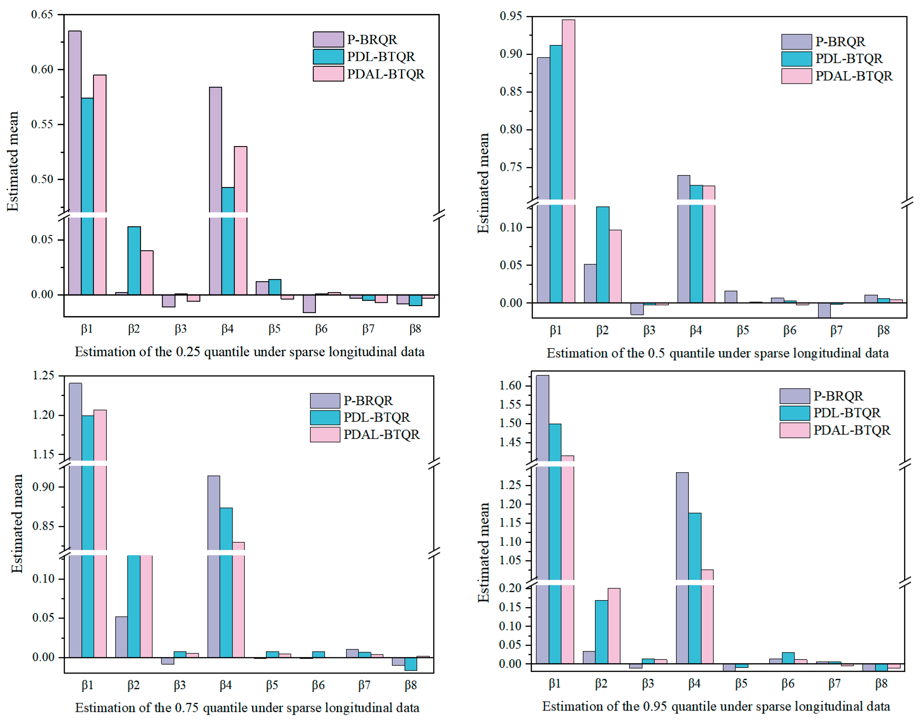
3.1.1. Simulation Results under Different Quartiles of Sparse Longitudinal Data

In the mixed-effects model, the double-penalized quantile regression method differs from existing studies in that both fixed effects and random effects have corresponding compression coefficients, thus eliminating irrelevant variables to a greater extent. In addition, this paper breaks with the existing literature by considering the estimation and selection of variables under the influence of different random effects only.

According to Figure 1, Figure 2 and Figure 3, the discussion is developed for sparse longitudinal data, and the interval censoring range is [0, 6]. At the lower quantile τ = 0.25, the lowest estimation error and fluctuations are observed from the MSE mean, and standard deviation metrics for the double adaptive Lasso penalty, i.e., the PDAL-BTQR method has the best estimation, and the redundant variables are almost all compressed to 0. At the middle quantile τ = 0.5, the MSEs mean obtained by the P-BTQR, PDL-BTQR, and PDAL-BTQR methods. The standard deviation of MSE for the P-BTQR method without penalty is two times that of the PDL-BTQR method and nearly three times that of the PDAL-BTQR method, which fully demonstrates the superiority of the two-penalty method for parameter estimation. At the middle and high quartiles τ = 0.75, the mean MSEs of the PDL-BTQR method and the PDAL-BTQR method are not significantly different, and the former is slightly higher than the latter, but both are smaller than the mean MSEs of the P-BTQR method. This means that both double-penalized methods can obtain accurate estimation results. At the high quantile τ = 0.95, the MSE means of the three methods are significantly higher, but the PDAL-BTQR method obtains the smallest MSE mean, standard deviation, and more accurate range of interval estimation in 100 simulations. In addition, in the model setting, assuming the explanatory variable coefficients β₁ and β₂ are disturbed by random effects, especially at the extreme quantile with the fluctuations of with are more obvious, indicating that their disturbances have the greatest impact on the estimation at the extreme quantile τ = 0.25 and τ = 0.95.

3.1.2. Simulation Results under Different Quartiles of Dense Longitudinal Data

According to Figure 4, Figure 5 and Figure 6, under the condition of dense longitudinal data, the estimation effect of the PDAL-BTQR method is better than that of the PDL-BTQR and P-BTQR methods at the lower quartile τ = 0.25, with the smallest MSE mean value of 0.062. At the middle quartile τ = 0.5 and the MSE mean value of the PDL-BTQR method is slightly lower than that of the PDAL-BTQR and P-BTQR methods. At the point where τ = 0.75, the MSE means of the double-punishment PDAL-BTQR and PDL-BTQR methods were smaller than those of the P-BTQR unpunished method, so the parameter estimation and variable selection of the unpunished method under this condition was not as good as those of the double-punished method. In terms of the mean and standard deviation of MSE, the estimation effects of the PDAL-BTQR method and the PDL-BTQR method were not significantly different and were similar to the results obtained in Table 1. At the high quantile, τ = 0.95, the mean square error of all three methods becomes relatively large, and the mean MSEs of the P-BTQR and PDL-BTQR methods are 0.245 and 0.201, respectively, while the mean MSE of the PDAL-BTQR method is 0.193, indicating that it has the best estimation effect of the dual adaptive Lasso at the high quantile.

In summary, it can be concluded that the double-penalized Bayesian Tobit quantile regression method can obtain more accurate parameter estimates for two different sets of explanatory variable coefficients at both low and high quantile points, and its performance is more advantageous than that of the no-penalty method, although the performance is comparable at the middle quantile point, but the accuracy of the double-penalized method is higher at the extreme quantile point.

3.2. Comparative Analysis of Simulation Results under Different Censoring Ratios

The estimation results of each method under different censoring ratios were compared by setting the censoring ratios to 10%, 20%, and 40%, respectively, keeping $\rho =0.5$, ${\epsilon }_{ij}~N\left(0,1\right)$, $D_1=diag\left(1,1,0\right)$ and taking $\tilde{N}=0$ and $\tilde{M}=3$ as constant. Since the estimation results of each quantile are similar,

Table 3. Estimation results for sparse longitudinal data with different censoring ratios.

Method	Estimation	MSE	β1	β2	β3	β4	β5	β6	β7	β8
			1	0	0	1	0	0	0	0
Censoring ratio = 10%
P-BTQR	Mean	0.029	0.846	−0.071	−0.008	0.931	−0.016	−0.006	0.013	−0.006
	Sd	0.026	0.232	0.242	0.127	0.138	0.116	0.129	0.120	0.115
	Confidence interval	-	[0.801, 0.891]	[−0.119, −0.023]	[−0.032, 0.016]	[0.904, 0.958]	[−0.039, 0.007]	[−0.031, 0.019]	[−0.011, 0.037]	[−0.028, 0.016]
PDL-BTQR	Mean	0.026	0.786	0.003	0.007	0.873	0.004	0.010	0.006	−0.003
	Sd	0.016	0.215	0.183	0.108	0.132	0.092	0.105	0.100	0.096
	Confidence interval	-	[0.744, 0.828]	[−0.032, 0.038]	[−0.014, 0.028]	[0.846, 0.900]	[−0.014, 0.022]	[−0.011, 0.031]	[−0.013, 0.025]	[−0.022, 0.016]
PDAL-BTQR	Mean	0.025	0.798	−0.024	−0.001	0.893	−0.004	0.003	0.006	0.007
	Sd	0.015	0.224	0.197	0.111	0.134	0.101	0.106	0.098	0.101
	Confidence interval	-	[0.755, 0.841]	[−0.063, 0.015]	[−0.023, 0.021]	[0.866, 0.920]	[−0.024, 0.016]	[−0.018, 0.024]	[−0.013, 0.025]	[−0.013, 0.027]
Censoring ratio = 20%
P-BTQR	Mean	0.030	0.866	−0.048	−0.013	0.901	−0.006	0.003	0.002	0.010
	Sd	0.018	0.228	0.248	0.123	0.162	0.129	0.124	0.126	0.118
	Confidence interval	-	[0.821, 0.911]	[−0.098, 0.002]	[−0.037, 0.011]	[0.868, 0.934]	[−0.031, 0.019]	[−0.022, 0.028]	[−0.022, 0.026]	[−0.013, 0.033]
PDL-BTQR	Mean	0.027	0.804	0.038	−0.001	0.840	0.000	0.011	0.005	0.006
	Sd	0.017	0.212	0.188	0.106	0.160	0.102	0.101	0.104	0.102
	Confidence interval	-	[0.763, 0.845]	[0.001, 0.075]	[−0.023, 0.021]	[0.808, 0.872]	[−0.020, 0.020]	[−0.009, 0.031]	[−0.014, 0.024]	[−0.014, 0.026]
PDAL-BTQR	Mean	0.026	0.840	−0.003	−0.007	0.864	−0.008	0.012	−0.001	0.009
	Sd	0.016	0.223	0.199	0.112	0.158	0.103	0.108	0.105	0.106
	Confidence interval	-	[0.797, 0.883]	[−0.042, 0.036]	[−0.029, 0.015]	[0.832, 0.896]	[−0.028, 0.012]	[−0.009, 0.033]	[−0.022, 0.020]	[−0.012, 0.030]
Censoring ratio = 40%
P-BTQR	Mean	0.033	0.867	−0.016	0.004	0.784	−0.014	−0.007	0.013	−0.007
	Sd	0.018	0.234	0.253	0.124	0.148	0.115	0.108	0.107	0.107
	Confidence interval	-	[0.821, 0.913]	[−0.068, 0.036]	[−0.019, 0.027]	[0.755, 0.813]	[−0.039, 0.008]	[−0.028, 0.014]	[−0.008, 0.034]	[−0.028, 0.014]
PDL-BTQR	Mean	0.032	0.811	0.074	0.007	0.729	−0.011	0.001	0.007	−0.006
	Sd	0.019	0.219	0.197	0.102	0.145	0.090	0.092	0.096	0.092
	Confidence interval	-	[0.769, 0.853]	[0.036, 0.112]	[−0.013, 0.027]	[0.700, 0.758]	[−0.028, 0.006]	[−0.017, 0.019]	[−0.011, 0.025]	[−0.024, 0.012]
PDAL-BTQR	Mean	0.031	0.833	0.033	0.003	0.743	−0.005	0.001	0.006	−0.001
	Sd	0.018	0.225	0.200	0.103	0.147	0.094	0.092	0.099	0.095
	Confidence interval	-	[0.789, 0.877]	[−0.006, 0.072]	[−0.017, 0.023]	[0.714, 0.772]	[−0.023, 0.013]	[−0.017, 0.019]	[−0.013, 0.025]	[−0.020, 0.018]

and

Table 4. Estimation results for dense longitudinal data with different censoring ratios.

Method	Estimation	MSE	β1	β2	β3	β4	β5	β6	β7	β8
			1	1	0.5	0.5	0.5	0.5	0.5	0.5
Censoring ratio = 10%
P-BTQR	Mean	0.042	0.810	0.787	0.441	0.492	0.431	0.464	0.474	0.459
	Sd	0.015	0.255	0.257	0.147	0.143	0.164	0.143	0.119	0.134
	Confidence interval	-	[0.759, 0.861]	[0.736, 0.838]	[0.413, 0.469]	[0.464, 0.520]	[0.399, 0.463]	[0.437, 0.491]	[0.450, 0.498]	[0.434, 0.484]
PDL-BTQR	Mean	0.040	0.793	0.826	0.444	0.466	0.428	0.435	0.459	0.441
	Sd	0.020	0.226	0.248	0.137	0.144	0.149	0.151	0.140	0.131
	Confidence interval	-	[0.748, 0.838]	[0.778, 0.874]	[0.417, 0.471]	[0.438, 0.494]	[0.399, 0.457]	[0.405, 0.465]	[0.433, 0.485]	[0.416, 0.466]
PDAL-BTQR	Mean	0.041	0.793	0.817	0.436	0.465	0.430	0.443	0.451	0.440
	Sd	0.021	0.235	0.256	0.140	0.150	0.160	0.149	0.140	0.139
	Confidence interval	-	[0.748, 0.838]	[0.766, 0.868]	[0.408, 0.464]	[0.435, 0.495]	[0.399, 0.461]	[0.413, 0.473]	[0.424, 0.478]	[0.413, 0.467]
Censoring ratio = 20%
P-BTQR	Mean	0.044	0.848	0.845	0.425	0.482	0.434	0.417	0.427	0.455
	Sd	0.019	0.269	0.286	0.160	0.171	0.155	0.136	0.151	0.127
	Confidence interval	-	[0.796, 0.900]	[0.789, 0.901]	[0.393, 0.457]	[0.448, 0.516]	[0.403, 0.465]	[0.391, 0.443]	[0.398, 0.456]	[0.430, 0.480]
PDL-BTQR	Mean	0.038	0.840	0.904	0.420	0.456	0.418	0.431	0.430	0.421
	Sd	0.020	0.233	0.258	0.143	0.157	0.145	0.138	0.151	0.131
	Confidence interval	-	[0.795, 0.885]	[0.852, 0.956]	[0.392, 0.448]	[0.426, 0.486]	[0.390, 0.446]	[0.402, 0.460]	[0.403, 0.457]	[0.395, 0.447]
PDAL-BTQR	Mean	0.039	0.841	0.890	0.418	0.453	0.422	0.421	0.434	0.439
	Sd	0.020	0.234	0.266	0.144	0.165	0.149	0.137	0.154	0.138
	Confidence interval	-	[0.796, 0.886]	[0.838, 0.942]	[0.389, 0.447]	[0.420, 0.486]	[0.393, 0.451]	[0.393, 0.449]	[0.404, 0.464]	[0.412, 0.466]
Censoring ratio = 40%
P-BTQR	Mean	0.048	0.793	0.830	0.375	0.388	0.362	0.355	0.371	0.382
	Sd	0.018	0.233	0.237	0.145	0.147	0.152	0.137	0.129	0.130
	Confidence interval	-	[0.748, 0.838]	[0.784, 0.876]	[0.346, 0.404]	[0.360, 0.416]	[0.332, 0.392]	[0.328, 0.382]	[0.345, 0.397]	[0.357, 0.407]
PDL-BTQR	Mean	0.046	0.794	0.876	0.373	0.382	0.356	0.374	0.371	0.374
	Sd	0.019	0.214	0.228	0.139	0.147	0.134	0.135	0.139	0.134
	Confidence interval	-	[0.752, 0.836]	[0.830, 0.922]	[0.346, 0.400]	[0.354, 0.410]	[0.329, 0.383]	[0.347, 0.401]	[0.345, 0.397]	[0.348, 0.400]
PDAL-BTQR	Mean	0.047	0.800	0.861	0.358	0.372	0.356	0.368	0.366	0.384
	Sd	0.021	0.209	0.237	0.145	0.148	0.145	0.131	0.140	0.135
	Confidence interval	-	[0.761, 0.839]	[0.815, 0.907]	[0.329, 0.387]	[0.343, 0.401]	[0.327, 0.385]	[0.342, 0.394]	[0.339, 0.393]	[0.358, 0.410]

only show the simulation results under 0.5 quantile.

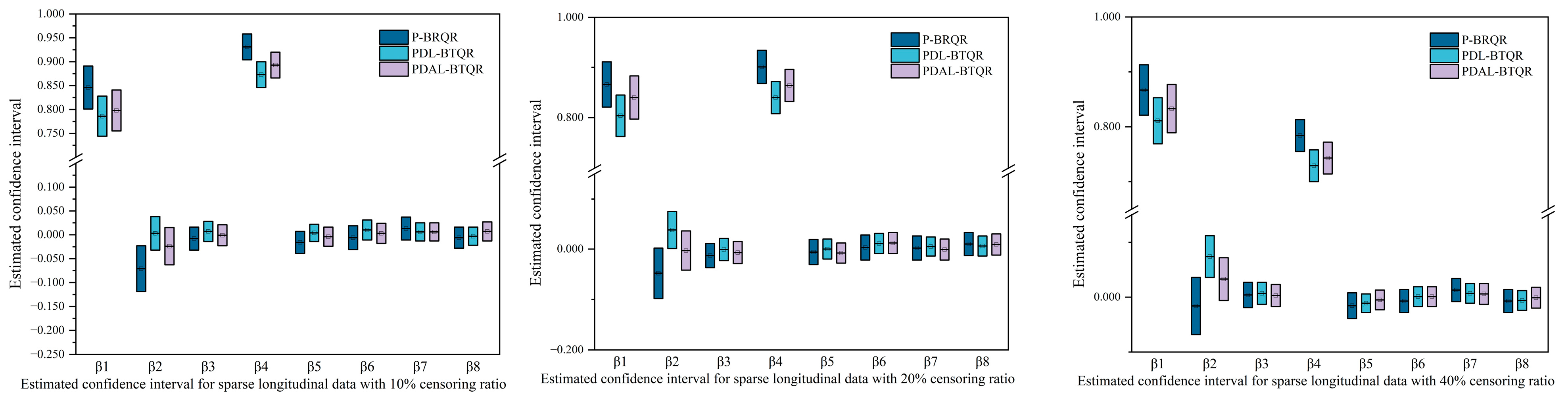
3.2.1. Simulation Results under Different Censoring Ratios of Sparse Longitudinal Data

According to Figure 7, Figure 8 and Figure 9, in the sparse longitudinal data model, with increasing censoring ratios, the mean MSE values for the P-BTQR method were 0.029, 0.030, and 0.033 for the three conditions comparing censoring ratios of 10%, 20%, and 30%, respectively; the mean MSE values for the PDL-BTQR method were 0.026, 0.027, and 0.032, respectively; and the mean MSE values for the PDAL-BTQR method were 0.025, 0.026, and 0.031, respectively. The mean MSE values corresponding to the three methods are reduced in order, because the Lasso quantile regression, compared to quantile regression, imposes a Lasso penalty on each explanatory variable, which can improve the speed of model calculation and reduce the bias of parameter estimation, and the results obtained from the simulation of the PDL-BTQR method are more accurate than those of the P-BTQR method, which is more accurate than the PDL-BTQR method. The adaptive Lasso penalty function breaks through this limitation. From the simulation results, the PDAL-BTQR method is more effective than the PDL-BTQR and P-BTQR methods for parameter estimation and variable selection under different censoring ratios.

3.2.2. Simulation Results under Different Censoring Ratios for Dense Longitudinal Data

According to Figure 10, Figure 11 and Figure 12, for dense longitudinal data, the mean MSEs of the P-BTQR, PDL-BTQR, and PDAL-BTQR methods are 0.042, 0.040, and 0.041, respectively, at a 10% censoring ratio, and the estimation method with a double Lasso penalty is more accurate. As the censoring ratio increases to 20%, the mean MSE of the P-BTQR method becomes larger while the mean MSEs of the PDL-BTQR and PDAL-BTQR methods decrease, which also indicates that the parameter estimation performance of the dual-penalty method is significantly better than that of the P-BTQR method. When the censoring ratio is further increased to 30%, the MSEs of all three methods increase, but the MSEs of the double-penalized PDL-BTQR and PDAL-BTQR methods are 0.046 and 0.047, respectively, which are still smaller than the MSE of the P-BTQR method of 0.048, indicating that the MSEs of the fixed-effects and random effects coefficients in the interval-censored mixed-effects model with double penalties are still smaller than the MSEs of the P-BTQR method. The estimation method for estimating the fixed-effects and random effects coefficients in the interval-censored mixed-effects model yields more accurate estimates of the model parameters. The PDL-BTQR method outperforms the other two methods for dense longitudinal data under the condition that the censoring ratio becomes larger, and the PDAL-BTQR method has the best estimation for sparse longitudinal data.

The MSE mean value increases correspondingly with the increase in the censoring proportion, implying that the estimation accuracy of fixed effects is decreasing, especially β₁ and β₂, which is the result of assuming the previous two variables subject are to random effects in this section during the simulation. Combining the simulation results of the coefficients of the two sets of explanatory variables, the PDL-BTQR method and the PDAL-BTQR method have better estimation results, and the advantages of their variable selection and estimation are more prominent than those of the P-BTQR method.

3.3. Comparative Analysis of Simulation Results under Different Random Error Distributions

Keeping $\rho =0.5$ and $D=diag\left(1,1,0\right)$ and taking $\tilde{N}=0$ and $\tilde{M}=6$ as constant, this paper will consider the variable selection and estimation results of three methods, P-BTQR, PDL-BTQR, and PDAL-BTQR, simulated under random errors obeying a standard normal distribution, a t(3) distribution, and an ALD(0,0.5,1) distribution, respectively. The advantage of the Bayesian-based framework is that the unknown parameters can be viewed as obeying a certain prior conditional distribution. After the prior conditional distributions of the different parameters to be estimated are given, the Gibbs sampling algorithm is used for parameter estimation and variable selection, and the estimation results under the 0.5 quantile are shown in

Table 5. Estimation results for sparse longitudinal data with different distributions.

Method	Estimation	MSE	β1	β2	β3	β4	β5	β6	β7	β8
			1	0	0	1	0	0	0	0
N(0,1)
P-BTQR	Mean	0.054	0.896	0.052	−0.015	0.740	0.016	0.007	−0.023	0.011
	Sd	0.141	0.311	0.330	0.125	0.246	0.172	0.137	0.116	0.117
	Confidence interval	-	[0.834, 0.958]	[−0.012, 0.116]	[−0.038, 0.008]	[0.690, 0.790]	[−0.017, 0.049]	[−0.021, 0.035]	[−0.044, −0.002]	[−0.011, 0.033]
PDL-BTQR	Mean	0.041	0.912	0.128	−0.002	0.727	0.000	0.003	−0.001	0.006
	Sd	0.070	0.263	0.273	0.101	0.204	0.106	0.102	0.092	0.098
	Confidence interval	-	[0.859, 0.965]	[0.075, 0.181]	[−0.021, 0.017]	[0.688, 0.766]	[−0.021, 0.021]	[−0.017, 0.023]	[−0.019, 0.017]	[−0.013, 0.025]
PDAL-BTQR	Mean	0.039	0.946	0.097	−0.002	0.726	0.002	−0.002	0.001	0.005
	Sd	0.052	0.283	0.248	0.104	0.207	0.100	0.099	0.092	0.095
	Confidence interval	-	[0.890, 1.002]	[0.049, 0.146]	[−0.023, 0.019]	[0.685, 0.767]	[−0.017, 0.021]	[−0.021, 0.017]	[−0.017, 0.019]	[−0.014, 0.024]
t(3)
P-BTQR	Mean	0.077	1.248	0.133	−0.029	0.944	−0.016	0.058	−0.075	0.006
	Sd	0.041	0.324	0.347	0.229	0.207	0.237	0.227	0.231	0.227
	Confidence interval	-	[1.186, 1.310]	[0.064, 0.202]	[−0.072, 0.015]	[0.903, 0.985]	[−0.061, 0.029]	[0.013, 0.103]	[−0.121, −0.029]	[−0.037, 0.049]
PDL-BTQR	Mean	0.057	1.178	0.250	0.010	0.918	0.022	0.051	−0.047	−0.003
	Sd	0.034	0.308	0.254	0.172	0.215	0.201	0.179	0.162	0.175
	Confidence interval	-	[1.120, 1.236]	[0.200, 0.300]	[−0.022, 0.042]	[0.877, 0.959]	[−0.017, 0.061]	[0.017, 0.085]	[−0.079, −0.015]	[−0.035, 0.029]
PDAL-BTQR	Mean	0.056	1.190	0.208	−0.009	0.901	0.008	0.044	−0.043	0.006
	Sd	0.033	0.305	0.257	0.168	0.201	0.201	0.189	0.178	0.178
	Confidence interval	-	[1.129, 1.251]	[0.158, 0.258]	[−0.042, 0.024]	[0.862, 0.940]	[−0.031, 0.047]	[0.008, 0.080]	[−0.077, −0.009]	[−0.027, 0.039]
ALD
P-BTQR	Mean	0.044	1.118	0.054	0.006	0.852	0.007	−0.022	−0.006	0.016
	Sd	0.028	0.327	0.306	0.123	0.173	0.128	0.152	0.138	0.134
	Confidence interval	-	[1.057, 1.179]	[−0.005, 0.113]	[−0.019, 0.031]	[0.818, 0.886]	[−0.018, 0.032]	[−0.051, 0.007]	[−0.033, 0.021]	[−0.010, 0.042]
PDL-BTQR	Mean	0.037	1.059	0.138	0.024	0.837	0.010	−0.012	0.007	0.004
	Sd	0.025	0.328	0.246	0.112	0.176	0.099	0.122	0.110	0.112
	Confidence interval	-	[0.997, 1.121]	[0.090, 0.186]	[0.002, 0.046]	[0.802, 0.872]	[−0.009, 0.029]	[−0.036, 0.012]	[−0.014, 0.028]	[−0.018, 0.026]
PDAL-BTQR	Mean	0.037	1.091	0.110	0.010	0.836	0.008	−0.022	0.007	0.001
	Sd	0.025	0.320	0.253	0.113	0.171	0.100	0.125	0.106	0.111
	Confidence interval	-	[1.029, 1.153]	[0.061, 0.159]	[−0.013, 0.033]	[0.802, 0.870]	[−0.012, 0.028]	[−0.046, 0.002]	[−0.013, 0.027]	[−0.021, 0.023]

and

Table 6. Estimation results for dense longitudinal data with different distributions.

Method	Estimation	MSE	β1	β2	β3	β4	β5	β6	β7	β8
			1	1	0.5	0.5	0.5	0.5	0.5	0.5
N(0,1)
P-BTQR	Mean	0.040	0.899	1.058	0.358	0.402	0.366	0.359	0.366	0.398
	Sd	0.018	0.237	0.243	0.126	0.146	0.143	0.136	0.127	0.126
	Confidence interval	-	[0.851, 0.947]	[1.011, 1.105]	[0.333, 0.383]	[0.374, 0.430]	[0.338, 0.394]	[0.332, 0.386]	[0.342, 0.390]	[0.373, 0.423]
PDL-BTQR	Mean	0.039	0.902	1.040	0.365	0.404	0.359	0.376	0.370	0.390
	Sd	0.018	0.227	0.230	0.129	0.138	0.138	0.138	0.131	0.129
	Confidence interval	-	[0.860, 0.944]	[0.996, 1.084]	[0.340, 0.390]	[0.377, 0.431]	[0.331, 0.387]	[0.349, 0.403]	[0.344, 0.396]	[0.365, 0.415]
PDAL-BTQR	Mean	0.040	0.905	1.013	0.352	0.395	0.367	0.365	0.362	0.382
	Sd	0.018	0.224	0.240	0.131	0.142	0.142	0.134	0.131	0.129
	Confidence interval	-	[0.861, 0.949]	[0.965, 1.061]	[0.326, 0.378]	[0.366, 0.424]	[0.339, 0.395]	[0.339, 0.391]	[0.336, 0.388]	[0.357, 0.407]
t(3)
P-BTQR	Mean	0.074	1.056	1.231	0.370	0.438	0.362	0.434	0.355	0.376
	Sd	0.041	0.293	0.323	0.215	0.214	0.213	0.218	0.218	0.214
	Confidence interval	-	[0.999, 1.113]	[1.171, 1.291]	[0.330, 0.410]	[0.397, 0.479]	[0.320, 0.404]	[0.391, 0.477]	[0.312, 0.398]	[0.335, 0.417]
PDL-BTQR	Mean	0.065	1.061	1.208	0.381	0.447	0.380	0.453	0.357	0.375
	Sd	0.034	0.280	0.293	0.199	0.205	0.200	0.208	0.208	0.204
	Confidence interval	-	[1.006, 1.116]	[1.152, 1.264]	[0.343, 0.419]	[0.407, 0.487]	[0.341, 0.419]	[0.413, 0.493]	[0.316, 0.398]	[0.336, 0.414]
PDAL-BTQR	Mean	0.068	1.039	1.184	0.350	0.425	0.346	0.424	0.335	0.354
	Sd	0.035	0.278	0.296	0.199	0.213	0.207	0.201	0.199	0.207
	Confidence interval	-	[0.984, 1.094]	[1.128, 1.240]	[0.312, 0.388]	[0.385, 0.465]	[0.306, 0.386]	[0.385, 0.463]	[0.300, 0.373]	[0.315, 0.393]
ALD
P-BTQR	Mean	0.046	1.011	1.155	0.400	0.411	0.419	0.374	0.414	0.410
	Sd	0.030	0.296	0.297	0.144	0.142	0.133	0.146	0.137	0.145
	Confidence interval	-	[0.953, 1.069]	[1.097, 1.213]	[0.372, 0.428]	[0.383, 0.439]	[0.393, 0.445]	[0.346, 0.402]	[0.387, 0.441]	[0.382, 0.438]
PDL-BTQR	Mean	0.043	1.022	1.133	0.407	0.422	0.416	0.402	0.406	0.397
	Sd	0.026	0.283	0.287	0.137	0.143	0.132	0.144	0.138	0.147
	Confidence interval	-	[0.968, 1.076]	[1.076, 1.190]	[0.381, 0.433]	[0.395, 0.449]	[0.391, 0.441]	[0.373, 0.431]	[0.379, 0.433]	[0.368, 0.426]
PDAL-BTQR	Mean	0.044	1.015	1.112	0.393	0.404	0.413	0.383	0.406	0.396
	Sd	0.025	0.282	0.279	0.142	0.148	0.139	0.153	0.148	0.151
	Confidence interval	-	[0.961, 1.069]	[1.056, 1.168]	[0.366, 0.420]	[0.375, 0.433]	[0.386, 0.440]	[0.354, 0.412]	[0.376, 0.436]	[0.367, 0.424]

.

3.3.1. Simulation Results under Different Random Error Distributions for Sparse Longitudinal Data

According to Figure 13, Figure 14 and Figure 15, from the estimation results of sparse longitudinal data with different random error distributions, when the random errors obey the standard normal distribution, the mean values of MSE estimated by the three methods P-BTQR, PDL-BTQR, and PDAL-BTQR are 0.054, 0.041, and 0.039, respectively, and all three methods can obtain the parameter estimation results with less deviation, but the PDL-BTQR method performs better than the P-BTQR method. Comparing the estimation results of the two double-penalty methods, the PDAL-BTQR method is superior, and its corresponding MSE standard deviation is the smallest at 0.052, indicating that the fluctuation of the 100 simulation results is smaller and its effect of obtaining accurate estimation is more stable. When the random errors obey the t(3) distribution, the mean MSE of the unpunished P-BTQR method increases significantly to 0.077, indicating that the parameter estimation results obtained by the P-BTQR method under the t(3) distribution are not as accurate as those under the standard normal distribution, while the corresponding mean MSEs of the PDL-BTQR method and the PDAL-BTQR method are 0.057 and 0.056, respectively, at this time. The difference between the two is not significant, which fully indicates that the estimation effect of the double-penalty method has obvious advantages. When the random errors obey the ALD(0,0.5,1) distribution, the estimation effects of the PDL-BTQR method and the PDAL-BTQR method are almost the same, and the mean MSE values are lower than those of the P-BTQR method. From the simulation results, the PDL-BTQR method and the PDAL-BTQR method perform better than the P-BTQR method regardless of the change in the random error.

3.3.2. Simulation Results under Different Random Error Distributions for Dense Longitudinal Data

According to Figure 16, Figure 17 and Figure 18, in the dense longitudinal data model, when the random errors obey the standard normal distribution, the MSEs obtained by the P-BTQR method and the PDAL-BTQR method have the same mean values, and both can obtain more accurate estimation results, and the PDL-BTQR method is better in comparison. When the random errors obey the t(3) distribution, similar to the results in Table 5, the mean MSE values of the three methods also increase significantly, but the P-BTQR method obtains the highest mean MSE value of 0.074, indicating that the estimation effect of the no-penalty method is poor, while the mean MSE values of the PDL-BTQR method and the PDAL-BTQR method are 0.065 and 0.068, respectively, indicating that the double-penalty method yields less biased parameter estimates. For the sparse longitudinal data, the mean MSEs of the PDL-BTQR and PDAL-BTQR methods are lower than those of the dense longitudinal data under the t(3) distribution, indicating that the dual-penalty method is more advantageous in handling the sparse longitudinal data. When the random errors obey the ALD(0,0.5,1) distribution, the mean MSE values obtained by the P-BTQR, PDL-BTQR, and PDAL-BTQR methods are 0.046, 0.043, and 0.044, respectively, and the two-penalty methods continue to perform better than the no-penalty methods. In addition, the simulation results show that the PDL-BTQR method has the best parameter estimation effect for processing dense longitudinal data under different random error distribution conditions.

In summary, the estimation error of the two-penalty Bayesian Tobit quantile regression method is the smallest regardless of whether the random errors obey the standard normal distribution or the t(3) distribution and the ALD(0,0.5,1) distribution. For different types of longitudinal data, the PDL-BTQR method and the PDAL-BTQR method both yield better parameter estimation and variable selection results for mixed-effects models with censored response variable intervals.

3.4. Time Consumption for the Methods

One important topic in modeling analysis is about the time required for computation. Although, with the advance in computer technology, the existing computational speed for much ordinary data can be handled comfortably, with the increasing requirements for model accuracy and the emergence of high-dimensional massive and complex data, computation time consumption is an issue of extreme concern even for the most advanced computers. The double-penalized Bayesian quantile regression method proposed in this study also involves large-scale operations. Below we use the sparse longitudinal data mixed-effects model from Section 3 to provide a demonstration of the various methods proposed in this thesis in terms of computing time. These methods include:

(1)

Unpenalized Bayesian Tobit quantile regression for interval-censored data (P-BTQR);

(2)

Single-Lasso penalized Bayesian Tobit quantile regression for interval-censored data (PL-BTQR);

(3)

Single-Adaptive Lasso penalized Bayesian Tobit quantile regression for interval-censored data (PAL-BTQR);

(4)

Double-Lasso penalized Bayesian Tobit quantile regression for interval-censored data (PDL-BTQR);

(5)

Double-Adaptive Lasso penalized Bayesian Tobit quantile regression for interval-censored data (PDAL-BTQR)

The prior settings in the Bayesian approach and the parameter settings in the double-penalized quantile regression are the same as in the previous simulations:

The number of iterations for all Bayesian methods was 20,000. The computer configuration is: Intel(R) Core (TM) 2 Duo CPU, 2.10 GHz, 2 G RAM; the running platform software is R software version 4.4.2, and the Bayesian methods all use the BUGS 1.4.

Table 7. Comparison of computational runtimes for different simulation methods based on Gibbs sampling.

Methods	User Time	System Time	Elapsed Time
P-BTQR	0.224	0.069	54.840
PL-BTQR	0.247	0.084	102.377
PAL-BTQR	0.219	0.043	104.179
PDL-BTQR	0.241	0.028	95.354
PDAL-BTQR	0.238	0.033	98.353

gives the average user time, system time and elapsed time of the above methods in 50 repetitions of simulation, all in seconds. Since, in the Bayesian method, we call the BUGS software, the user time and system time do not include the real sampling time of the calculation, so here we compare the total running time as more appropriate.

The double-penalized Bayesian method is slightly shorter in running time than the single-penalized method and it offers greater advantages in practical applications. Since the dual-penalty method is able to consider the effects of both fixed and random effects and penalize them appropriately, it can provide more accurate parameter estimates and more reliable prediction results. In addition, the dual-penalty method is capable of automatic variable selection and parameter compression, which further improves the generalization ability and interpretability of the model.

In summary, the dual-penalty method provides more accurate parameter estimates and more reliable prediction results while maintaining a similar runtime as the single-penalty method. This makes the double-penalized Bayesian Tobit quantile regression method an attractive option, especially when dealing with complex data and constructing high-precision models.

4. Interprovincial Longitudinal Crime Rate Data Analysis

The Bayesian double-penalty-based longitudinal interval-censored data quantile regression method studied in this paper may be more suitable for the case where the dependent variables are not categorical variables data, with higher model accuracy and better variable selection and model estimation in continuous-type data.

Currently, many scholars at home and abroad have conducted more in-depth empirical studies on the relationship between crime rates and some conventional economic indicators, such as regional income disparity, urbanization, and unemployment rate, which are important reasons for the rise of crime rate indicators [29]. Based on the study of Monte Carlo simulation analysis in the previous section, this section will discuss the relationship between crime rates and economic indicator data for 31 provinces across the country from 2010 to 2016 using the two new methods, PDL-BTQR and PDAL-BTQR, which contain 1302 observations; 31 provinces across the country were classified into eastern, central and western regions. The conclusion found that crime rates were higher in the eastern and western regions than in the central region, suggesting a correlation with regional income disparities at this stage of the country’s history.

Since the crime rate is expressed by the number of crimes with approved arrests per 10,000 people, using it as a response variable will be limited by the left-hand side being greater than 0. Secondly, in this section, we will select the top 10 regions with high crime rates in the eastern and western regions, calculate the average crime rate of these 10 regions, and use the average crime rate as the upper limit of the response variable to obtain the upper limit of the response variable of 9.35. Therefore, the crime rate is a set of response variable bilaterally constrained data, i.e., between [0, 9.35], the censored rate is 12.9%.

According to previous studies, scholars have studied the main causes of rising crime rates from several perspectives, including total economy, urban population, education, wealth gap, and employment. Therefore, this section identifies the explanatory variables as: gross per capita product, urbanization rate, regional income gap, education level, and unemployment rate. Among them, the crime rate data are obtained from the Chinese Prosecution Yearbook and the Chinese Law Yearbook, and the economic indicators are obtained from the Chinese Statistical Yearbook. The specific variable definitions and descriptive statistics are shown in

Table 8. Variable definitions and descriptive statistics.

Variant	Name	Define	Mean	Sd	Max	Min
Y	Crime rate	Number of criminal suspects arrested by the Public Prosecutor’s Office per 10,000 population	6.684	2.301	14.840	3.549
X1	Per capita GDP	GDP output per unit of population	4.277	2.088	12.319	1.299
X2	Urbanization rate	Ratio of regional urban population to total population	0.543	0.137	0.896	0.222
X3	Regional income gap	Difference between per capita disposable income of regional residents and per capita disposable income of national residents	0.545	0.543	3.048	0.002
X4	Educational level	Average number of students enrolled in higher education per 100,000 population	0.247	0.086	0.620	0.108
X5	Unemployment rate	Urban registered unemployment rate	3.369	0.654	4.500	1.200

. To provide insight into the relationship between the variables in the dataset, analysis of correlation coefficients and covariances was introduced and the results are displayed in Figure 19 and Figure 20.

Utilizing equation $\{\begin{array}{l}{y}_{ij}^{\ast }=x_{ij}^{\prime }\beta +z_{ij}^{\prime }{\alpha }_i+{\epsilon }_{ij}\\ y_{ij}=y_{ij}^{\ast }\cdot I\left( \tilde{\mathrm{N}}\le y_{ij}^{\ast }\le \tilde{M}\right)+\tilde{M}I\left(y_{ij}^{\ast }>\tilde{M}\right)+ \tilde{\mathrm{N}}I\left(y_{ij}^{\ast }< \tilde{\mathrm{N}}\right)\end{array}$ for the interval-censored model; among these, the response variable y_ij denotes the value of the crime rate of the i-th province in the j-th year, $i=31$ and $j=7$; $y_{ij}^{\ast }$ is a latent variable.${\mathrm{x}}_{ij}^{\prime }=\left(1, {\mathrm{x}}_{1ij}^{\prime }, {\mathrm{x}}_{2ij}^{\prime }, {\mathrm{x}}_{3ij}^{\prime }, {\mathrm{x}}_{4ij}^{\prime }, {\mathrm{x}}_{5ij}^{\prime }\right)$ for the intercept distance term and five explanatory variables; among them $x_{1ij}^{\prime }$, $x_{2ij}^{\prime }$, $x_{3ij}^{\prime }$, $x_{4ij}^{\prime }$, $x_{5ij}^{\prime }$ are the observed values of the relevant explanatory variables for the i-th province in the j-th year, respectively. β = (β₀, β₀, …, β₀)′ are the coefficients of each explanatory variable; α_i is the random effects coefficient; $z_{ij}^{\prime }$ denotes an explanatory variable that produces a random effect and ${\mathrm{z}}_{ij}^{\prime }\subset x_{ij}^{″}$, assuming that ${\mathrm{z}}_{ij}^{\prime }=x_{ij}^{\prime }$.

We are interested in the degree of influence of each explanatory variable on the response variable at different quantile points, and

Table 9. Estimates of the two methods at different quartiles.

Variant	$\mathit{\tau }=0.1$	$\mathit{\tau }=0.2$	$\mathit{\tau }=0.3$	$\mathit{\tau }=0.4$	$\mathit{\tau }=0.5$	$\mathit{\tau }=0.6$	$\mathit{\tau }=0.7$	$\mathit{\tau }=0.8$	$\mathit{\tau }=0.9$
PDL-BTQR
Per capita GDP	−0.097	−0.079	−0.060	−0.068	−0.099	−0.134	−0.153	−0.117	−0.010
Urbanization rate	0.456	0.423	0.406	0.424	0.449	0.442	0.380	0.334	0.264
Regional income disparities	0.161	0.178	0.175	0.182	0.201	0.232	0.273	0.229	0.125
Educational level	−0.399	−0.366	−0.359	−0.392	−0.428	−0.430	−0.413	−0.358	−0.298
Unemployment rate	−0.102	−0.117	−0.135	−0.171	−0.211	−0.240	−0.249	−0.212	−0.151
PDAL-BTQR
Per capita GDP	−0.162	−0.129	−0.111	−0.119	−0.153	−0.195	−0.230	−0.208	−0.046
Urbanization rate	0.610	0.581	0.536	0.546	0.572	0.563	0.510	0.473	0.356
Regional income disparities	0.187	0.199	0.206	0.212	0.240	0.281	0.319	0.277	0.169
Educational level	−0.592	−0.592	−0.585	−0.602	−0.646	−0.643	−0.630	−0.556	−0.475
Unemployment rate	−0.126	−0.149	−0.166	−0.190	−0.239	−0.257	−0.259	−0.218	−0.163

shows the estimation results of both the PDL-BTQR and PDAL-BTQR methods at each quantile point.

Table 8 shows that GDP per capita, education level, and unemployment rate are inversely related to crime rate at each quantile, i.e., as the regional GDP per capita, education level, and unemployment rate increase, they effectively suppress the increase in crime rate, especially the education level, whose estimated coefficients at each quantile are larger in absolute value than GDP per capita and unemployment rate. The urbanization rate and regional income disparity act as positive shocks to crime rates, i.e., an increase in the urbanization rate and an increase in income disparity both lead to an increase in crime rates, and both estimation methods indicate that the urbanization rate reaches a maximum at the 0.5 quantile and the income disparity has the greatest impact at the 0.7 quantile. A high urbanization rate responds to a certain extent to the high mobility of the mobile population, which is more likely to breed crime, while an increase in regional income disparity and a widening gap between rich and poor in the region can easily cause class conflicts, trigger social unrest, and generate delinquent behavior. In the real data, the estimation of the model and variable selection in this paper are performed simultaneously, and the penalty part enables automatic variable selection.

5. Discussion

In this paper, considering the situation that the response variable is restricted by the bilateral limit, we construct a double-penalized Bayesian Tobit quantile regression model for interval-censored data, add the penalty function to the fixed-effect and random-effect coefficients at the same time, make parameter estimation and variable selection of the interval-censored mixed-effects model, and obtain the estimation results of the two sets of longitudinal data in a Monte Carlo simulation under different estimation methods, different censoring ratios, and different random error distributions, and use the new method to analyze and discuss the correlation between crime rate and various economic indicators in China. The Monte Carlo simulation is used to obtain the estimation results of the two sets of longitudinal data under different estimation methods, different censoring ratios, and different random error distributions.

In the mixed-effects model with censored data, the general Tobit quantile regression method cannot obtain effective estimation of the parameters [1]. On the one hand, due to the random effects added to the mixed-effects model on the basis of the general linear model [30], there are a large number of unknown parameters and the distribution of random errors is unknown, and the random errors under different distributions will increase the complexity of the model computation, which will bring great difficulties to the model parameter estimation; on the other hand, due to the restricted response variable generating a large number of censored data, the mixed-effects model contains latent variables that make the Markov Chain of the parameter estimation Monte Carlo (MCMC) sampling algorithm for parameter estimation extremely complex, resulting in low computational efficiency and a large bias in the estimation results. In recent years, parameter estimation and variable selection based on the idea of a penalty function under the Bayesian framework is one of the hot topics of academic discussion [1]. Therefore, on the basis of existing research, in order to solve the above problems, this paper is devoted to constructing a Bayesian double-penalty Tobit quantile regression model for censored data, so as to provide a new way of thinking for the parameter estimation and variable selection methods of censored mixed-effects models [31].

For interval-censored data, Richard Cox proposed the Cox PH model in 1972 [32], which is mainly used to study the relationship between multiple independent variables and the dependent variable (survival time) and can handle censored data, which is highly practical. Cox proportional risk model may not be the best choice when the data are truncated and an explicit concept of survival time does not exist. This paper discusses the parameter estimation and variable selection under the condition that the response variable is subject to bilateral restrictions at the same time. Due to the characteristics of boundedness and bias of interval-censored data [33], the estimation results of simple regression methods cannot effectively screen important variables and exclude redundant variables [34]. The main reason is that the fitted and estimated values obtained by traditional regression methods may exceed the upper and lower bounds of the response variables, and the model interpretation is relatively weak [35]. The Tobit quantile regression method provides a new way of parameter estimation for the mixed-effects model with interval-censored response variables [36]. Therefore, this paper firstly combines the Bayesian method and constructs the Bayesian empirical likelihood function under interval-censored data [37]. Secondly, the penalty function is introduced, and a more efficient Gibbs sampling algorithm is constructed using the truncated normal distribution of the asymmetric Laplace prior part [38]. Finally, Monte Carlo simulation experiments and real data analysis are carried out, which fully illustrate the advantages of Bayesian double-penalty Tobit quantile regression model such as high estimation efficiency and robustness.

However, although this paper proposes the double-penalized Bayesian Tobit quantile regression method for the mixed-effects model with censored data and constructs the Gibbs sampling algorithm for parameter estimation, and the simulation results confirm that the estimation effect of the new method is better than that of the traditional method, there are still some shortcomings. This paper only analyzes the Lasso penalty and adaptive Lasso penalty for the commonly used variable selection methods, and subsequently can use SCAD, elastic net, adaptive elastic net, and other penalty methods for parameter estimation and variable selection; this paper centers on the study of linear models and subsequently can construct a Bayesian Tobit quantile regression model for the censored data under the nonlinear model and explore the nonlinear model’s variable selection problem.

6. Conclusions

This paper proposes a Bayesian double-penalized Tobit quantile regression method for interval-censored data in mixed-effects models. The method compresses the fixed and random effects parameters using an unconditional Laplace prior to improve the estimation accuracy. The posterior distributions are derived from a mixture of truncated normal distributions and a Gibbs sampling algorithm is constructed for parameter estimation. Both simulation and real data analysis show that the method outperforms traditional methods in parameter estimation and variable selection, and is particularly suitable for dealing with censored data.

(1)

Significantly improved model accuracy and efficiency

In complex mixed-effects models, the double-penalty approach of PDL-BTQR and PDAL-BTQR effectively reduces the estimation error of the model and improves the accuracy of parameter estimation by compressing the random effects coefficients. This approach significantly improves the predictive power and interpretability of the model by simultaneous parameter estimation and variable selection when dealing with longitudinal data, regardless of whether the data are sparse or dense. In addition, this dual-penalty strategy helps to identify and exclude redundant variables, thus further optimizing the model structure.

(2)

Demonstrated robustness in handling complex and variable datasets

In practical applications, data often have different censoring ratios and complex random error distributions. In this case, the dual-penalty method shows good robustness. Whether facing high censoring ratios or different random error distributions, the dual-penalty approach provides stable parameter estimation and accurate variable selection. In particular, the PDL-BTQR method excels when dealing with dense longitudinal data, while the PDAL-BTQR method is even better when dealing with sparse longitudinal data. This robustness makes the dual-penalty method widely applicable and flexible in practical applications.

(3)

New and effective tool for dealing with interval-censored data

In statistics and data analysis, interval-censored data is a common and complex data type. Traditional treatments often make it difficult to accurately estimate parameters and make effective variable selection. However, the model proposed in this study is particularly suitable for dealing with interval-censored data, and its superiority in parameter estimation and variable selection is verified by setting a bilateral truncation of the response variable and conducting a simulation study, and the model is able to realize automatic variable selection. A new effective method is provided for dealing with data with censored characteristics.

References

1. Song, X.K.; Ming, T. Marginal Models for Longitudinal Continuous Proportional Data. Biometrics 2000, 56, 496–502. [Google Scholar] [CrossRef] [PubMed]
2. Ferrari, S.; Cribari-Neto, F. Beta Regression or Modeling Rates and Proportions. J. Appl. Stat. 2004, 31, 799–815. [Google Scholar] [CrossRef]
3. Lesaffre, E.; Rizopoulos, D.; Tsonaka, R. The logistic transform for bounded outcomes scores. Biostatistics 2007, 8, 72–85. [Google Scholar] [CrossRef] [PubMed]
4. Espinheira, P.L.; Ferrari, S.L.P.; Cribari-Neto, F. Infuence diagnostics in beta regression. Comput. Stat. Data Anal. 2008, 52, 4417–4431. [Google Scholar] [CrossRef]
5. Zhao, W.; Zhang, R.; Lv, Y.; Liu, J. Variable selection for varying dispersion beta regression model. J. Appl. Stat. 2014, 41, 95–108. [Google Scholar] [CrossRef]
6. Ying, Z.L.; Yu, W.; Zhao, Z.Q.; Zheng, M. Regression Analysis of Doubly Truncated Data. J. Am. Stat. Assoc. 2019, 115, 810–821. [Google Scholar] [CrossRef] [PubMed]
7. Tobin, J. Estimation of relationships for limited dependent variables. Econometrica 1958, 26, 24–36. [Google Scholar] [CrossRef]
8. Cunha Danúbia, R.; Angelo, J.D.; Helton, S. On a log-symmetric quantile Tobit model applied to female labor supply data. J. Appl. Stat. 2022, 49, 4225–4253. [Google Scholar] [CrossRef]
9. Powell, J.L. Censored regression quantiles. J. Econom. 1986, 32, 143–155. [Google Scholar] [CrossRef]
10. Frumento, P. A quantile regression estimator for interval-censored data. Int. J. Biostat. 2023, 19, 81–96. [Google Scholar] [CrossRef]
11. Li, L.; Hao, R.; Yang, X. Data Augmentation Based Quantile Regression Estimation for Censored Partially Linear Additive Model. Comput. Econ. 2023, 1–30. [Google Scholar] [CrossRef]
12. Hao, R.; Weng, C.; Liu XYang, X. Data augmentation based estimation for the censored quantile regression neural network model. Expert Syst. Appl. 2023, 214, 119097. [Google Scholar] [CrossRef]
13. Yu, R.; Long, X.; Quddus, M.; Wang, J.H. A Bayesian Tobit quantile regression approach for naturalistic longitudinal driving capability assessment. Accid. Anal. Prev. 2020, 147, 105779. [Google Scholar] [CrossRef] [PubMed]
14. Tibshirani, R.J. Regression shrinkage and selection via the lasso. J. R. Stat. Soc. Ser. B Stat. Methodol. 1996, 58, 267–288. [Google Scholar] [CrossRef]
15. Fan, J.; Li, R. Variable Selection via Non-concave Penalized Likelihood and Its Oracle Properties. J. Am. Stat. Assoc. 2001, 96, 1348–1360. [Google Scholar] [CrossRef]
16. Kim, S.M.; Lee, S.B.; Lee, S.H.; Kim, W. Robust estimation of outage costs in South Korea using a machine learning technique: Bayesian Tobit quantile regression. Appl. Energy 2020, 278, 115702. [Google Scholar] [CrossRef]
17. Alhamzawi, R.; Keming, Y.; Dries, F.B. Bayesian adaptive Lasso quantile regression. Stat. Model. 2012, 12, 279–297. [Google Scholar] [CrossRef]
18. Alhamzawi, R. Bayesian Elastic Net Tobit Quantile Regression. Commun. Stat.—Simul. Comput. 2016, 45, 2409–2427. [Google Scholar] [CrossRef]
19. Alhusseini, F. New Bayesian Lasso in Tobit Quantile Regression. Rom. Statal Rev. Suppl. 2017, 65, 213–229. [Google Scholar]
20. Alhamzawi, R.; Ali, M.T.H. Bayesian tobit quantile regression with penalty. Commun. Stat.—Simul. Comput. 2018, 47, 1739–1750. [Google Scholar] [CrossRef]
21. Abbas, H.K. Bayesian Lasso Tobit regression. J. Al-Qadisiyah Comput. Sci. Math. 2019, 11, 1–13. [Google Scholar] [CrossRef]
22. Kottas, A.; Krnjaji, M. Bayesian Semiparametric Modelling in Quantile Regression. Scand. J. Stat. 2009, 36, 297–319. [Google Scholar] [CrossRef]
23. Narjes, G.; Reza, P. The likelihood and Bayesian analyses for asymmetric Laplace nonlinear regression model. Comput. Appl. Math. 2024, 43, 21. [Google Scholar]
24. Mallows, D.F.; Andrews, L. Scale Mixtures of Normal Distributions. J. R. Stat. Soc. Ser. B Methodol. 1974, 36, 99–102. [Google Scholar]
25. Zou, H. The Adaptive Lasso and Its Oracle Properties. J. Am. Stat. Assoc. 2006, 101, 1418–1429. [Google Scholar] [CrossRef]
26. Alhamzawi, R.; Yu, K. Bayesian Lasso-mixed Quantile Regression. J. Stat. Comput. Simul. 2012, 84, 868–880. [Google Scholar] [CrossRef]
27. Luo, Y.X.; Li, H.F. The Research of Double Adaptive Lasso Quantile Regression Model with Random Effects. J. Quant. Technol. Econ. 2017, 34, 136–148. [Google Scholar]
28. Alhamzawi, R.; Ali, H.T.M. The Bayesian adaptive lasso regression. Math. Biosci. 2018, 303, 75–82. [Google Scholar] [CrossRef]
29. Bhattacharya, A. Analysis of the Factors Affecting Violent Crime Rates in the US. Int. J. Eng. Manag. Res. 2020, 10, 106–109. [Google Scholar] [CrossRef]
30. Shen, P.S. Median regression model with left truncated and interval-censored data. J. Korean Stat. Soc. 2013, 42, 469–479. [Google Scholar] [CrossRef]
31. Zhou, X.; Feng YDu, X. Quantile regression for interval censored data. Commun. Stat.-Theory Methods 2017, 46, 3848–3863. [Google Scholar] [CrossRef]
32. Cox David, R. Regression models and life-tables. J. R. Stat. Soc. Ser. B 1972, 34, 187–202. [Google Scholar]
33. Angelov, A.G.; Magnus, E.; Klarizze, P.; Arcenas, A.; Bengt, K. Quantile regression with interval-censored data in questionnaire-based studies. Comput. Stat. 2022, 39, 583–603. [Google Scholar] [CrossRef]
34. Dengluan, D.; Anmin, T.; Jinli, Y. High-Dimensional Variable Selection for Quantile Regression Based on Variational Bayesian Method. Mathematics 2023, 11, 2232. [Google Scholar] [CrossRef]
35. Wang, Z.F.; Li, T.; Xiao, L.Q.; Tu, D.S. A threshold longitudinal Tobit quantile regression model for identification of treatment-sensitive subgroups based on interval-bounded longitudinal measurements and a continuous covariate. Stat. Med. 2023, 42, 4618–4631. [Google Scholar] [CrossRef]
36. Wang, Z.Q.; Wu, Y.; Cheng, W.L. Variational inference on a Bayesian adaptive lasso Tobit quantile regression model. Stat 2023, 12, 13. [Google Scholar] [CrossRef]
37. Kobayashi, G. Bayesian Endogenous Tobit Quantile Regression. Bayesian Anal. 2017, 12, 161–191. [Google Scholar] [CrossRef]
38. Alhusseini, H.H.F.; Georgescu, V. Bayesian composite Tobit quantile regression. J. Appl. Stat. 2017, 45, 727–739. [Google Scholar] [CrossRef]
Figure 1. Estimated mean of three methods for different quartiles under sparse longitudinal data.
Mathematics 12 01782 g001
Figure 2. Estimated standard deviation of three methods for different quartiles under sparse longitudinal data.
Mathematics 12 01782 g002
Figure 3. Estimated confidence interval of three methods for different quartiles under sparse longitudinal data.
Mathematics 12 01782 g003
Figure 4. Estimated means of three methods for different quartiles under dense longitudinal data.
Mathematics 12 01782 g004
Figure 5. Estimated standard deviations of three methods for different quartiles under dense longitudinal data.
Mathematics 12 01782 g005
Figure 6. Estimated confidence intervals of three methods for different quartiles under dense longitudinal data.
Mathematics 12 01782 g006
Figure 7. Estimated means for sparse longitudinal data with different censoring ratios.
Mathematics 12 01782 g007
Figure 8. Estimated standard deviations for sparse longitudinal data with different censoring ratios.
Mathematics 12 01782 g008
Figure 9. Estimated confidence intervals for sparse longitudinal data with different censoring ratios.
Mathematics 12 01782 g009
Figure 10. Estimated means for dense longitudinal data with different censoring ratios.
Mathematics 12 01782 g010
Figure 11. Estimated standard deviations for dense longitudinal data with different censoring ratios.
Mathematics 12 01782 g011
Figure 12. Estimated confidence intervals for dense longitudinal data with different censoring ratios.
Mathematics 12 01782 g012
Figure 13. Estimated means for sparse longitudinal data with different distributions.
Mathematics 12 01782 g013
Figure 14. Estimated standard deviations for sparse longitudinal data with different distributions.
Mathematics 12 01782 g014
Figure 15. Estimated confidence intervals for sparse longitudinal data with different distributions.
Mathematics 12 01782 g015
Figure 16. Estimated means for dense longitudinal data with different distributions.
Mathematics 12 01782 g016
Figure 17. Estimated standard deviations for dense longitudinal data with different distributions.
Mathematics 12 01782 g017
Figure 18. Estimated confidence intervals for dense longitudinal data with different distributions.
Mathematics 12 01782 g018
Figure 19. Heat map between variables.
Mathematics 12 01782 g019
Figure 20. Network diagram of covariance between variables.
Mathematics 12 01782 g020