Matrix Pencil Optimal Iterative Algorithms and Restarted Versions for Linear Matrix Equation and Pseudoinverse

Abstract

We derive a double-optimal iterative algorithm (DOIA) in an m-degree matrix pencil Krylov subspace to solve a rectangular linear matrix equation. Expressing the iterative solution in a matrix pencil and using two optimization techniques, we determine the expansion coefficients explicitly, by inverting an $m\times m$ positive definite matrix. The DOIA is a fast, convergent, iterative algorithm. Some properties and the estimation of residual error of the DOIA are given to prove the absolute convergence. Numerical tests demonstrate the usefulness of the double-optimal solution (DOS) and DOIA in solving square or nonsquare linear matrix equations and in inverting nonsingular square matrices. To speed up the convergence, a restarted technique with frequency m is proposed, namely, DOIA(m); it outperforms the DOIA. The pseudoinverse of a rectangular matrix can be sought using the DOIA and DOIA(m). The Moore–Penrose iterative algorithm (MPIA) and MPIA(m) based on the polynomial-type matrix pencil and the optimized hyperpower iterative algorithm OHPIA(m) are developed. They are efficient and accurate iterative methods for finding the pseudoinverse, especially the MPIA(m) and OHPIA(m).

1. Introduction

Since pioneering works [1,2], Krylov subspace methods have been studied and developed extensively in the iterative solution of linear equations systems [3,4,5,6,7,8,9], like the minimum residual algorithm [10], the generalized minimal residual method (GMRES) [6,7], the quasiminimal residual method [8], the biconjugate gradient method [11], the conjugate gradient squared method [12], and the biconjugate gradient stabilized method [13]. For more discussion on the Krylov subspace methods, one can refer to review papers [5,14,15] and text books [16,17].

In this paper, we use the matrix pencil Krylov subspace method to derive some novel numerical algorithms to solve the following linear matrix equation:

$$AZ=F,$$

(1)

where $Z\in {\mathbb{R}}^{n\times p}$ is an unknown matrix. We consider two possible cases:

$$\begin{array}{ccc}\hfill & & \mathrm{Case} 1:A\in {\mathbb{R}}^{n\times n},F\in {\mathbb{R}}^{n\times p},\hfill \end{array}$$

(2)

$$\begin{array}{ccc}\hfill & & \mathrm{Case} 2:A\in {\mathbb{R}}^{q\times n},F\in {\mathbb{R}}^{q\times p}.\hfill \end{array}$$

(3)

We assume $\mathrm{rank}\left(A\right)=\mathrm{rank}\left[AF\right]$ for consistency in Equation (1).

The problem of solving a matrix equation is one of the most important topics in computational mathematics and has been widely studied in many different fields. As shown by Jbilou et al. [18], there are many methods for solving square linear matrix equations. Many iterative algorithms based on the block Krylov subspace method have been developed to solve matrix equations [19,20,21]. For a multiple-righthand-side system with A being nonsingular, the block Krylov subspace methods for computing $A^{-1}F$ in Equation (1) comprise an even larger body of the literature [22,23,24]. There are some novel algorithms for solving Equation (1) with nonsquare A and square Z in [25,26,27,28]. Having an effective and fast solution to matrix equations plays a fundamental role in numerous fields of science. To reduce the computational complexity and increase the accuracy, a more efficient method is still required.

One of the applications of Equation (1) is finding the solution to the following linear equation system:

$$Ax=b.$$

(4)

It is noted that for the solution to Equation (4), we need to find the left inversion of A, which is denoted by $A_L^{-1}$. When we take $F=I_n$, Equation (1) is used to find the right inversion of A, which is denoted by $A_R^{-1}$. Mathematically, $A_L^{-1}=A_R^{-1}$ for nonsingular square matrices; however, from the numerical outputs, $A_L^{-1}\ne A_R^{-1}$, especially for ill-conditioned matrices.

In order to find the left inversion of A, we can solve

$$XA=I_n;$$

(5)

a transpose leads to

$$A^{\mathrm{T}}{X}^{\mathrm{T}}=I_n.$$

(6)

If we use $A^{\mathrm{T}}$ to replace A, then we supply an optimal solution and optimal iterative scheme to seek $X^{\mathrm{T}}$; inserting its transpose into Equation (4), we can obtain the solution of x with

$$x=Xb.$$

(7)

There are many algorithms for finding $A_L^{-1}$ or $A_R^{-1}$ for nonsingular matrices. Liu et al. [29] modified the conjugate gradient (CG)-type method to the matrix conjugate gradient method (MCGM), which performed well in finding the inverse matrix. Other iterative schemes encompass the Newton–Schultz method [30], the Chebyshev method [31], the Homeier method [32], the method by Petkovic and Stanimirovic [33], and some cubic and higher-order convergence methods [34,35,36,37].

We can apply Equation (1) to find a pseud-inverse $A^{†}$ with dimensions $n\times q$ of a rectangular matrix A with dimensions $q\times n$:

$$A{A}^{†}=I_q,$$

(8)

where $I_q$ is a q-dimensional identity matrix. This is a special Case 2 in Equation (3) with $p=q$ and $F=I_q$.

For wide application, the pseudoinverse and the Moore–Penrose inverse matrices have been investigated and computed using many methods [33,34,35,36,37,38,39,40,41,42,43,44,45]. More higher-order iterative schemes for the Moore–Penrose inverse were recently analyzed by Sayevand et al. [46].

In order to compare different solvers for systems of nonlinear equations, some novel goodness and qualification criteria are defined in [47]. They include convergence order, number of function evaluations, number of iterations, CPU time, etc., for evaluating the quality of a proposed iterative method.

From Equation (1),

$$B=F-A{Z}_0$$

(9)

is an initial residual matrix, if an initial guess $Z_0$ is given. Let

$$X=Z-Z_0.$$

(10)

Then, Equation (1) is equivalent to

$$AX=B,$$

(11)

which is used to search a descent direction X after giving an initial residual. It follows from Equations (9) and (10) that

$$R=F-AZ=B-AX$$

(12)

is a residual matrix. Below we will develop novel method to solve Equation (11), and hence Equation (1), if we replace B by F and Z by X. Since we cannot find the exact solutions of Equations (1) and (11) in general, the residual R in Equation (12) is not zero.

1.1. Notation

Throughout this paper, uppercase letters denote matrices, while lowercase letters denote vectors or scalars. If two matrices A and B have the same order, their inner product is defined by $A:B=tr\left(A^{\mathrm{T}}B\right)$, where $tr$ is the trace of a square matrix, and the superscript T signifies the transpose. As a consequence, the Frobenius norm of A is given by ${\parallel A\parallel }^2:=tr\left(A^{\mathrm{T}}A\right)=A:A$. The component of a vector a is written as $a_i$, while the component of a matrix A is written as $A_{ij}$. A single subscript k in a matrix $U_k$ means that it is the kth matrix in a matrix pencil.

1.2. Main Contribution

In GMRES [16], an m-dimensional matrix Krylov subspace is supposed,

$${\mathcal{K}}_m(A,B):=\mathrm{Span}\{B,AB,\dots ,A^{m-1}B\}.$$

(13)

The Petrov–Galerkin method searches $X\in {\mathcal{K}}_m$ via a perpendicular property:

$$B-AX\perp {\mathcal{L}}_m=A{\mathcal{K}}_m.$$

(14)

The descent matrix $X\in {\mathcal{K}}_m$ can be achieved by minimizing the residual [16]:

$${min\parallel R\parallel }^2=min{\parallel B-AX\parallel }^2.$$

(15)

Equation (14) is equivalent to the projection of B on ${\mathcal{L}}_m$, and R is perpendicular to ${\mathcal{L}}_m$. To seek a fast convergent iterative algorithm, we must keep the orthogonality and simultaneously maximize the projection quantity:

$$max\frac{{[B:\left(AX\right)]}^2}{{\parallel AX\parallel }^2}.$$

(16)

The main contribution of this paper is that we seek the best descent matrix X simultaneously satisfying (15) and (16). Some excellent properties including the absolute convergence of the proposed iterative algorithm are proven. When the matrix Krylov subspace method in Equation (13) is not suitable for the Case 2 problem, we can treat both Case 1 and 2 problems of linear matrix equations in a unified manner. Now, our problem is to construct double-optimal iterative algorithms with an explicit expansion form to solve the linear matrix Equation (1), which involves inverting a low-dimensional $m\times m$ positive definite matrix. Our problem is more difficult than that using (15) to derive iterative algorithms of the GMRES type. For the pseudoinverse problem of a rectangular matrix, higher-order polynomial methods and hyperpower iterative algorithms are unified into the frame of a double-optimal matrix pencil method but with different matrix pencils.

1.3. Outline

We start from an m-degree matrix pencil Krylov subspace to express the solution to the linear matrix equation in Section 2; two cases of linear matrix equations are considered. In Section 3, two merit functions are optimized for the determination of the expansion coefficients. More importantly, an explicit form double-optimal solution (DOS) to Equation (11) is created, for which we needed to invert an $m\times m$ positive definite matrix. In Section 4, we propose an iterative algorithm updated using the DOS method, which provides the best descent direction used in the double-optimal iterative algorithm (DOIA). A restarted version with frequency m, namely, the DOIA(m) is proposed. The DOS can be viewed as a single-step DOIA. Linear matrix equations are solved by the DOS, DOIA, and DOIA(m) methods in Section 5 to display some advantages of the presented methodology to find the approximate solution of Equation (1). The Moore–Penrose inverse of a rectangular matrix is addressed in Section 6, proposing two optimized methods based on a new matrix pencil of polynomials and a new modification of the hyperpower method. Numerical testing of the Moore–Penrose inverse of rectangular matrix is carried out in Section 7. Finally, the conclusions are drawn in Section 8.

2. The Matrix Pencil Krylov Subspace Method

This section constructs suitable bases for Case 1 and Case 2 problems of the linear matrix Equation (1). We denote the expansion space with $\mathrm{Span}\{U_0,\mathcal{U}\}$. For Case 1,

$$\begin{array}{ccc}\hfill & & U_0=B,\hfill \end{array}$$

(17)

$$\begin{array}{ccc}\hfill & & \mathcal{U}:=[U_1,\dots ,U_m]=[A{U}_0,\dots ,A^m{U}_0],\hfill \end{array}$$

(18)

while, for Case 2,

$$\begin{array}{ccc}\hfill & & U_0=A^{\mathrm{T}}B,\hfill \end{array}$$

(19)

$$\begin{array}{ccc}\hfill & & \mathcal{U}:=[U_1,\dots ,U_m]=[A^{\mathrm{T}}A{U}_0,\dots ,{\left(A^{\mathrm{T}}A\right)}^m{U}_0].\hfill \end{array}$$

(20)

In $\mathcal{U}$, the matrices $U_1,\dots ,U_m$ are orthonormalized by using the modified Gram–Schmidt process, such that $U_i:U_j={\delta }_{ij}$, where : denotes the inner product of $U_i$ and $U_j$.

In the space of $\mathrm{Span}\{U_0,\mathcal{U}\}$, X in Equation (11) can be expanded as

$$X={\alpha }_0{U}_0+\sum _{k=1}^m{\alpha }_k{U}_k={\alpha }_0{U}_0+\mathcal{U}\alpha ,$$

(21)

where $\alpha :={({\alpha }_1,\dots ,{\alpha }_m)}^{\mathrm{T}}$. The coefficients ${\alpha }_0$ and $\alpha$ are determined optimally from a combination of $U_0\in {\mathbb{R}}^{n\times p}$ and the m matrix $U_k\in {\mathbb{R}}^{n\times p},k=1,\dots ,m$ in a degree m matrix pencil Krylov subspace.

Both Case 1 and Case 2 can be treated in a unified manner as shown below, but with different $U_0$ and $\mathcal{U}$. $\mathcal{U}$ is a matrix pencil consisting of m matrices in the matrix Krylov subspace, and $\mathcal{U}\alpha$ is the product of the pencil with vector $\alpha \in {\mathbb{R}}^m$. For the frequent use of the later, we give a definition of $\mathcal{U}\alpha$ as

$$\mathcal{U}\alpha :=\sum _{j=1}^m{\alpha }_j{U}_j.$$

(22)

In Equation (21), X is spanned by $\{U_0,\mathcal{U}\}$, and we may write it as $X\in \mathrm{Span}\{U_0,\mathcal{U}\}$. So, we call our expansion method a degree $m+1$ matrix- pencil Krylov subspace method. It is different from the fixed affine matrix Krylov subspace $X\in U_0+\mathrm{Span}\left\{\mathcal{U}\right\}$. The concept of fixed and varying affine Krylov subspaces was elaborated in [48].

3. Double-Optimal Solution

In this section, we seek the best descent matrix X simultaneously satisfying (15) and (16). The properties including the orthogonality of residual and absolute convergence of the proposed iterative algorithm are proven. We must emphasize that the derived iterative algorithms have explicit expansion forms to solve the linear matrix Equation (11), by inverting an $m\times m$ positive definite matrix.

3.1. Two Minimizations

To simplify the notation, let

$$Y:=AX;$$

(23)

we consider the orthogonal projection of B to Y, measured by the error matrix:

$$E:=B-B:\left(\frac{Y}{\parallel Y\parallel }\right)\frac{Y}{\parallel Y\parallel }.$$

(24)

The best approximation of X in Equation (11) can be found, when $Y=AX$ minimizes

$${\parallel E\parallel }^2={\parallel B\parallel }^2-\frac{{(B:Y)}^2}{{\parallel Y\parallel }^2}\ge 0,$$

(25)

or maximizes the orthogonal projection of B to Y:

$$\underset{Y}{max}\left\{\frac{{(B:Y)}^2}{{\parallel Y\parallel }^2}\right\}.$$

(26)

We can solve $AX=B$ by an approximation of X from the above optimization technique, but $B-AX$ is not exactly equal to zero, since $Y=AX$ involves the unknown matrix X, and Y is not exactly equal to B.

Let

$$f:=\frac{{\parallel Y\parallel }^2}{{(B:Y)}^2}\ge \frac{1}{{\parallel B\parallel }^2},$$

(27)

which is the reciprocal of the merit function in Equation (26).

Let

$$Y_j=A{U}_j.$$

(28)

Then, Equation (23), with the aid of Equation (21), can be written as

$$Y=Y_0+\mathcal{Y}\alpha ,$$

(29)

where

$$\begin{array}{ccc}\hfill & & Y_0:={\alpha }_{0}A{U}_0,\hfill \end{array}$$

(30)

$$\begin{array}{ccc}\hfill & & \mathcal{Y}:=[Y_1,\dots ,Y_m]=A\mathcal{U}=[A{U}_1,\dots ,A{U}_m];\hfill \end{array}$$

(31)

$\mathcal{Y}$ is an m-degree matrix-pencil. We suppose that for each $Y_j,j=1,\dots ,m$, rank$\left(Y_j\right)=min[n,p]$ for Case 1, and rank$\left(Y_j\right)=min[q,p]$ for Case 2. We take rank$\left(Y_j\right)=n_0$, where $n_0=min[n,p]$ for Case 1, and $n_0=min[q,p]$ for Case 2.

Inserting Equation (29) for Y into Equation (27), we encounter the following minimization problem:

$$\underset{\alpha }{min}\left\{f=\frac{{\parallel Y\parallel }^2}{{(B:Y)}^2}=\frac{\parallel Y_0{+\mathcal{Y}\alpha \parallel }^2}{{[B:Y_0+B:\left(\mathcal{Y}\alpha \right)]}^2}\right\};$$

(32)

however, in Y there is still an unknown scalar ${\alpha }_0$ in $Y_0={\alpha }_{0}A{U}_0$. Other minimization of the residual is supplemented:

$$\underset{{\alpha }_0}{min}{\{\parallel R\parallel }^2={\parallel B-AX\parallel }^2={\parallel B-Y\parallel }^2\}.$$

(33)

The solution of these two optimization problems is a major task at the next subsection.

3.2. Two Main Theorems

The first theorem determines the expansion coefficients ${\alpha }_j,j=0,1,\dots ,m$ in Equation (21).

Theorem 1.

For $X\in Span\{U_0,\mathcal{U}\}$, the optimal solution of Equation (11) derived from the optimizations in (32) and (33) is given by

$$X={\alpha }_0[U_0+{\lambda }_0\mathcal{U}Dv-\mathcal{U}Du],$$

(34)

where

$$\begin{array}{ccc}\hfill & & C=\left[C_{ij}\right],C_{ij}=Y_i:Y_j,\hfill \\ & & D=C^{-1},\hfill \\ & & v=\left[v_i\right],v_i=B:Y_i,\hfill \\ & & u=\left[u_i\right],u_i=\left(A{U}_0\right):Y_i,\hfill \\ & & {\lambda }_0=\frac{\parallel A{U}_0{\parallel }^2-u^{T}Du}{B:\left(A{U}_0\right)-v^{T}Du},\hfill \\ & & W={\lambda }_0\mathcal{Y}Dv-\mathcal{Y}Du+A{U}_0,\hfill \\ & & {\alpha }_0=\frac{W:B}{{\parallel W\parallel }^2}.\hfill \end{array}$$

(35)

We suppose that rank$\left(C\right)=m<n_0$, such that $C^{-1}$ exists.

Proof. 

With the help of Equation (29), $B:Y$ in (32) can be written as

$$B:Y=B:Y_0+v^{\mathrm{T}}\alpha ,$$

(36)

where the components of $v\in {\mathbb{R}}^m$ are given by

$$v_i:=B:Y_i.$$

(37)

Taking the squared norms of Equation (29) yields

$${\parallel Y\parallel }^2=\parallel Y_0{+\mathcal{Y}\alpha \parallel }^2={\parallel Y_0\parallel }^2+2{(Y_0:\mathcal{Y})}^{\mathrm{T}}\alpha +{\alpha }^{\mathrm{T}}\mathcal{Y}:\mathcal{Y}\alpha ,$$

where $\mathcal{Y}:\mathcal{Y}=Y_i:Y_j,i,j=1,\dots ,m$ is an $m\times m$ matrix. We can derive

$${\parallel Y\parallel }^2={\parallel Y_0\parallel }^2+2w^{\mathrm{T}}\alpha +{\alpha }^{\mathrm{T}}C\alpha ,$$

(38)

where

$$\begin{array}{ccc}\hfill & & w_i:=Y_0:Y_i,\hfill \end{array}$$

(39)

$$\begin{array}{ccc}\hfill & & C_{ij}=Y_i:Y_j;\hfill \end{array}$$

(40)

$w\in {\mathbb{R}}^m$ and $C\in {\mathbb{R}}^{m\times m}$ is a symmetric positive definite matrix.

The minimality condition of f is

$${\nabla }_{\alpha }\frac{{\parallel Y\parallel }^2}{{(B:Y)}^2}=0\Rightarrow {(B:Y)}^2{y}_2-2B:Y{\parallel Y\parallel }^2{y}_1=0,$$

(41)

where

$$\begin{array}{ccc}\hfill & & y_1:={\nabla }_{\alpha }(B:Y)=v,\hfill \end{array}$$

(42)

$$\begin{array}{ccc}\hfill & & y_2:={\nabla }_{\alpha }{\parallel Y\parallel }^2=2w+2C\alpha ;\hfill \end{array}$$

(43)

$y_1$ and $y_2$ are m-vectors, while $C>0\in {\mathbb{R}}^{m\times m}$ with rank$\left(C\right)=m$. Thus, the equation to determine $\alpha$ is

$$B:Y{y}_2-2{\parallel Y\parallel }^2{y}_1=0.$$

(44)

We can observe from Equation (44) that $y_2$ is proportional to $y_1$, which is supposed to be

$$y_2=2\lambda y_1,$$

(45)

where $\lambda$ is a multiplier to be determined from

$${\parallel Y\parallel }^2=\lambda B:Y.$$

(46)

Then, it follows from Equations (42), (43) and (45) that

$$\begin{array}{ccc}\hfill & & w+C\alpha =\lambda v,\hfill \end{array}$$

(47)

$$\begin{array}{ccc}\hfill & & \alpha =\lambda Dv-Dw,\hfill \end{array}$$

(48)

where

$$D:=C^{-1}>0\in {\mathbb{R}}^{m\times m}.$$

(49)

Inserting Equation (48) into Equations (36) and (38), we have

$$\begin{array}{ccc}\hfill & & B:Y=B:Y_0+\lambda v^{\mathrm{T}}Dv-v^{\mathrm{T}}Dw,\hfill \end{array}$$

(50)

$$\begin{array}{ccc}\hfill & & {\parallel Y\parallel }^2={\lambda }^2{v}^{\mathrm{T}}Dv+{\parallel Y_0\parallel }^2-w^{\mathrm{T}}Dw.\hfill \end{array}$$

(51)

Inserting Equations (50) and (51) into Equation (46) yields

$${\lambda }^2{v}^{\mathrm{T}}Dv+{\parallel Y_0\parallel }^2-w^{\mathrm{T}}Dw=\lambda B:Y_0+{\lambda }^2{v}^{\mathrm{T}}Dv-\lambda v^{\mathrm{T}}Dw.$$

Cancelling ${\lambda }^2{v}^{\mathrm{T}}Dv$ on both sides, we can derive

$$\parallel Y_0{\parallel }^2-w^{\mathrm{T}}Dw=\lambda [B:Y_0-v^{\mathrm{T}}Dw],$$

(52)

which renders

$$\lambda =\frac{\parallel Y_0{\parallel }^2-w^{\mathrm{T}}Dw}{B:Y_0-v^{\mathrm{T}}Dw}.$$

(53)

Inserting it into Equation (48), $\alpha$ is obtained as follows:

$$\alpha =\frac{\parallel Y_0{\parallel }^2-w^{\mathrm{T}}Dw}{B:Y_0-v^{\mathrm{T}}Dw}Dv-Dw.$$

(54)

Let

$$u_i:=\left(A{U}_0\right):Y_i.$$

(55)

Inserting Equation (30) for $Y_0={\alpha }_{0}A{U}_0$ into Equation (39), and comparing it to Equation (55), we have

$$w_i={\alpha }_0{u}_i⟹w={\alpha }_{0}u.$$

(56)

By inserting $\alpha$ in Equation (48) into Equation (21) and using $Y_0={\alpha }_{0}A{U}_0$, we can obtain

$$X={\alpha }_0{U}_0+\lambda \mathcal{U}Dv-\mathcal{U}Dw={\alpha }_0{U}_0+{\alpha }_0\mathcal{U}z,$$

(57)

where

$$\begin{array}{ccc}\hfill & & z:={\lambda }_{0}Dv-Du,\hfill \end{array}$$

(58)

$$\begin{array}{ccc}\hfill & & {\lambda }_0:=\frac{\parallel A{U}_0{\parallel }^2-u^{\mathrm{T}}Du}{B:\left(A{U}_0\right)-v^{\mathrm{T}}Du},\hfill \end{array}$$

(59)

$$\begin{array}{ccc}\hfill & & \lambda =\frac{\parallel Y_0{\parallel }^2-w^{\mathrm{T}}Dw}{B:Y_0-v^{\mathrm{T}}Dw}={\alpha }_0{\lambda }_0.\hfill \end{array}$$

(60)

Upon letting

$$V:=U_0+\mathcal{U}z,$$

(61)

Equation (57) can be expressed as

$$X={\alpha }_{0}V.$$

(62)

Now ${\alpha }_0$ can be determined by (33). Inserting Equation (62) into (33) yields

$${\parallel B-AX\parallel }^2=\parallel B-{\alpha }_0{AV\parallel }^2={\alpha }_0^2{\parallel W\parallel }^2-2{\alpha }_{0}W:B+{\parallel B\parallel }^2,$$

(63)

where

$$W:=AV=A{U}_0+\mathcal{Y}z={\lambda }_0\mathcal{Y}Dv-\mathcal{Y}Du+A{U}_0$$

(64)

is derived according to Equations (31) and (58).

Differentiating Equation (63) vs ${\alpha }_0$ and equating it to zero, generates

$${\alpha }_0=\frac{W:B}{{\parallel W\parallel }^2};$$

(65)

by Equation (62),

$$X=\frac{W:B}{{\parallel W\parallel }^2}V.$$

(66)

The proof of Theorem 1 is complete.   □

To prove Theorem 2, we need the following two lemmas.

Lemma 1.

In terms of the matrix-pencil $\mathcal{Y}$ in Equation (31), we have

$$\begin{array}{ccc}\hfill & & B:\left(\mathcal{Y}Dv\right)=v^{T}Dv,\hfill \end{array}$$

(67)

$$\begin{array}{ccc}\hfill & & B:\left(\mathcal{Y}Du\right)=v^{T}Du.\hfill \end{array}$$

(68)

Proof. 

By using the definition in Equation (22), the left-hand side of Equation (67) can be written as

$$B:\left(\mathcal{Y}Dv\right)=B:\left(\sum _{j=1}^m{\left(Dv\right)}_j{Y}_j\right)=\sum _{j=1}^m{\left(Dv\right)}_{j}B:Y_j=\sum _{j=1}^m{v}_j{\left(Dv\right)}_j,$$

where $v_j$ and ${\left(Dv\right)}_j$ denote, respectively, the jth component of v and $Dv$, and Equation (37) is used in the last equality. In terms of vector form the last term is just the right-hand side of Equation (67). Similarly, Equation (68) can be proved by the same manner, i.e.,

$$B:\left(\mathcal{Y}Du\right)=B:\left(\sum _{j=1}^m{\left(Du\right)}_j{Y}_j\right)=\sum _{j=1}^m{\left(Du\right)}_{j}B:Y_j=\sum _{j=1}^m{v}_j{\left(Du\right)}_j.$$

This ends the proof of Lemma 1.   □

Lemma 2.

In terms of the matrix-pencil $\mathcal{Y}$ in Equation (31), we have

$$\left(A{U}_0\right):\left(\mathcal{Y}z\right)=u^{T}z.$$

(69)

Proof. 

By using the definition in Equation (22), the left-hand side of Equation (69) can be written as

$$\left(A{U}_0\right):\left(\mathcal{Y}z\right)=\left(A{U}_0\right):\left(\sum _{j=1}^m{z}_j{Y}_j\right)=\sum _{j=1}^m{z}_j\left(A{U}_0\right):Y_j=\sum _{j=1}^m{z}_j{u}_j,$$

where $z_j$ and $u_j$ denote, respectively, the jth component of z and u, and Equation (55) is used in the last equality. In terms of vector form the last term is just the right-hand side of Equation (69). This ends the proof of Lemma 2.   □

Theorem 2.

In Theorem 1, the two parameters ${\alpha }_0$ and ${\lambda }_0$ satisfy the following reciprocal relation:

$$\lambda ={\alpha }_0{\lambda }_0=1.$$

(70)

Proof. 

Taking the inner product of B with Equation (64) and by Lemma 1, leads to

$$B:W={\lambda }_0{v}^{\mathrm{T}}Dv+B:\left(A{U}_0\right)-v^{\mathrm{T}}Du.$$

(71)

With the aid of Equation (59), we have

$$B:W={\lambda }_0{v}^{\mathrm{T}}Dv+\frac{1}{{\lambda }_0}[\parallel A{U}_0{\parallel }^2-u^{\mathrm{T}}Du].$$

(72)

Then after multiplying ${\lambda }_0$ on the above equation, and by Equation (65), we can obtain

$${\alpha }_0{\lambda }_0{\parallel W\parallel }^2={\parallel A{U}_0\parallel }^2+{\lambda }_0^2{v}^{\mathrm{T}}Dv-u^{\mathrm{T}}Du.$$

(73)

Next we prove that Equation (73) is equal to ${\parallel W\parallel }^2$. From Equation (64) and with the aids of Equations (40), (58) and (69), it follows that

$$\begin{array}{ccc}\hfill {\parallel W\parallel }^2& =& \parallel A{U}_0{\parallel }^2+2\left(A{U}_0\right):\left(\mathcal{Y}z\right)+z^{\mathrm{T}}Cz\hfill \\ & =& \parallel A{U}_0{\parallel }^2+2u^{\mathrm{T}}z+z^{\mathrm{T}}Cz\hfill \\ & =& \parallel A{U}_0{\parallel }^2+2{\lambda }_0{u}^{\mathrm{T}}Dv-2u^{\mathrm{T}}Du+({\lambda }_0{v}^{\mathrm{T}}D-u^{\mathrm{T}}D)C({\lambda }_{0}Dv-Du)\hfill \\ & =& \parallel A{U}_0{\parallel }^2+{\lambda }_0^2{v}^{\mathrm{T}}Dv-u^{\mathrm{T}}Du,\hfill \end{array}$$

(74)

where $DCD=D$ was used in view of Equation (49). Then by comparing Equations (73) and (74), we have proven Equation (70). This ends the proof of ${\alpha }_0{\lambda }_0=1$. Then by Equation (60), $\lambda =1$ is proven.   □

A more direct proof of $\lambda =1$ is available by comparing Equation (46) to Equation (96), which is derived in the proof of Theorem 4.

3.3. Estimating Residual Error

To estimate the residual error we begin with the following lemma.

Lemma 3.

In terms of the matrix-pencil $\mathcal{Y}$ in Equation (31), we have

$$\begin{array}{ccc}\hfill & & \left(A{U}_0\right):\left(\mathcal{Y}Dv\right)=u^{T}Dv,\hfill \end{array}$$

(75)

$$\begin{array}{ccc}\hfill & & \left(A{U}_0\right):\left(\mathcal{Y}Du\right)=u^{T}Du.\hfill \end{array}$$

(76)

Proof. 

By using the definition in Equations (22) and (55), the left-hand side of Equation (75) can be written as

$$\left(A{U}_0\right):\left(\mathcal{Y}Dv\right)=\left(A{U}_0\right):\left(\sum _{j=1}^m{\left(Dv\right)}_j{Y}_j\right)=\sum _{j=1}^m{\left(Dv\right)}_j\left(A{U}_0\right):Y_j=\sum _{j=1}^m{u}_j{\left(Dv\right)}_j,$$

where $u_j$ and ${\left(Dv\right)}_j$ denote, respectively, the jth component of u and $Dv$. In terms of vector form the last term is just the right-hand side of Equation (75). Similarly, Equation (76) can be proved by the same manner, i.e.,

$$\left(A{U}_0\right):\left(\mathcal{Y}Du\right)=\left(A{U}_0\right):\left(\sum _{j=1}^m{\left(Du\right)}_j{Y}_j\right)=\sum _{j=1}^m{\left(Du\right)}_j\left(A{U}_0\right):Y_j=\sum _{j=1}^m{u}_j{\left(Du\right)}_j.$$

This ends the proof of Lemma 3.   □

Lemma 4.

In terms of the matrix-pencil $\mathcal{Y}$ in Equation (31), we have

$$\begin{array}{ccc}\hfill & & \left(\mathcal{Y}Du\right):\left(\mathcal{Y}Du\right)=u^{T}Du,\hfill \end{array}$$

(77)

$$\begin{array}{ccc}\hfill & & \left(\mathcal{Y}Dv\right):\left(\mathcal{Y}Dv\right)=v^{T}Dv,\hfill \end{array}$$

(78)

$$\begin{array}{ccc}\hfill & & \left(\mathcal{Y}Du\right):\left(\mathcal{Y}Dv\right)=u^{T}Dv.\hfill \end{array}$$

(79)

Proof. 

By using the definition in Equation (22), we have

$$\left(\mathcal{Y}Du\right):\left(\mathcal{Y}Du\right)=\left({\left(Du\right)}_i{Y}_i\right):\left({\left(Du\right)}_j{Y}_j\right)={\left(Du\right)}_i{\left(Du\right)}_j{Y}_i:Y_j.$$

(80)

The above two repeated indices i and j are summed automatically from 1 to m according to the convention of Einstein [49]. Then with the aid of Equation (40), we have

$$\left(\mathcal{Y}Du\right):\left(\mathcal{Y}Du\right)=\left({\left(Du\right)}_i{Y}_i\right):\left({\left(Du\right)}_j{Y}_j\right)={\left(Du\right)}_i{C}_{ij}{\left(Du\right)}_j=u_i{D}_{ij}{u}_j,$$

(81)

where $D=C^{-1}$ was used. In terms of vector form the above equation leads to Equation (77). Similarly, we have

$$\begin{array}{ccc}\hfill & & \left(\mathcal{Y}Dv\right):\left(\mathcal{Y}Dv\right)={\left(Dv\right)}_i{C}_{ij}{\left(Dv\right)}_j=v_i{D}_{ij}{v}_j,\hfill \end{array}$$

(82)

$$\begin{array}{ccc}\hfill & & \left(\mathcal{Y}Du\right):\left(\mathcal{Y}Dv\right)={\left(Du\right)}_i{C}_{ij}{\left(Dv\right)}_j=u_i{D}_{ij}{v}_j.\hfill \end{array}$$

(83)

In terms of vector form the above two equations reduce to Equations (78) and (79). This ends the proof of Lemma 4.   □

Theorem 3.

For $X\in Span\{U_0,\mathcal{U}\}$, the residual error of the optimal solution in Equation (57) satisfies:

$${\parallel B-AX\parallel }^2={\parallel B\parallel }^2-v^{T}Dv-\frac{{[B:\left(A{U}_0\right)-v^{T}Du]}^2}{\parallel A{U}_0{\parallel }^2-u^{T}Du}.$$

(84)

Proof. 

According to Equation (70), we can refine X in Equation (34) to

$$X={\alpha }_0[U_0-\mathcal{U}Du]+\mathcal{U}Dv,$$

(85)

where

$${\alpha }_0=\frac{B:\left(A{U}_0\right)-v^{\mathrm{T}}Du}{\parallel A{U}_0{\parallel }^2-u^{\mathrm{T}}Du}.$$

(86)

Let us check residual square:

$${\parallel B-AX\parallel }^2={\parallel B-Y\parallel }^2={\parallel Y\parallel }^2-2B:Y+{\parallel B\parallel }^2,$$

(87)

where

$$Y=AX={\alpha }_{0}A{U}_0-{\alpha }_0\mathcal{Y}Du+\mathcal{Y}Dv$$

(88)

is obtained from Equation (85), in which $\mathcal{Y}=A\mathcal{U}$.

By using Lemmas 1, 3 and 4, it follows from Equation (88) that

$$\begin{array}{ccc}\hfill & & {\parallel Y\parallel }^2={\alpha }_0^2(\parallel A{U}_0{\parallel }^2-u^{\mathrm{T}}Du)+v^{\mathrm{T}}Dv,\hfill \end{array}$$

(89)

$$\begin{array}{ccc}\hfill & & B:Y={\alpha }_{0}B:\left(A{U}_0\right)-{\alpha }_0{v}^{\mathrm{T}}Du+v^{\mathrm{T}}Dv.\hfill \end{array}$$

(90)

Equation (90) is easily derived by taking the inner product of B to Equation (88):

$$B:Y={\alpha }_{0}B:\left(A{U}_0\right)-{\alpha }_{0}B:\mathcal{Y}Du+B:\mathcal{Y}Dv,$$

and using Lemma 1. Taking the squared norms of Equation (88), we have

$$\begin{array}{ccc}& & {\parallel Y\parallel }^2={\parallel {\alpha }_{0}A{U}_0-{\alpha }_0\mathcal{Y}Du+\mathcal{Y}Dv\parallel }^2\hfill \\ & & ={\alpha }_0^2\parallel A{U}_0{\parallel }^2+{\alpha }_0^2{\parallel \mathcal{Y}Du\parallel }^2+{\parallel \mathcal{Y}Dv\parallel }^2\hfill \\ & & -2{\alpha }_0^2\left(A{U}_0\right):\left(\mathcal{Y}Du\right)+2{\alpha }_0\left(A{U}_0\right):\left(\mathcal{Y}Dv\right)-2{\alpha }_0\left(\mathcal{Y}Du\right):\left(\mathcal{Y}Dv\right);\hfill \end{array}$$

by using Lemmas 3 and 4, it is simplified to

$$\begin{array}{ccc}& & {\parallel Y\parallel }^2={\alpha }_0^2{\parallel A{U}_0\parallel }^2+{\alpha }_0^2{u}^{\mathrm{T}}Du+v^{\mathrm{T}}Dv\hfill \\ & & -2{\alpha }_0^2{u}^{\mathrm{T}}Du+2{\alpha }_0{u}^{\mathrm{T}}Dv-2{\alpha }_0{u}^{\mathrm{T}}Dv={\alpha }_0^2{\parallel A{U}_0\parallel }^2-{\alpha }_0^2{u}^{\mathrm{T}}Du+v^{\mathrm{T}}Dv.\hfill \end{array}$$

It derives Equation (89).

Then, inserting the above two equations into Equation (87), we have

$$\begin{array}{ccc}\hfill & & {\parallel B-AX\parallel }^2={\alpha }_0^2(\parallel A{U}_0{\parallel }^2-u^{\mathrm{T}}Du)+v^{\mathrm{T}}Dv-2{\alpha }_{0}B:\left(A{U}_0\right)+2{\alpha }_0{v}^{\mathrm{T}}Du-2v^{\mathrm{T}}Dv+{\parallel B\parallel }^2\hfill \\ & & ={\alpha }_0^2(\parallel A{U}_0{\parallel }^2-u^{\mathrm{T}}Du)+2{\alpha }_0[v^{\mathrm{T}}Du-B:\left(A{U}_0\right)]+{\parallel B\parallel }^2-v^{\mathrm{T}}Dv.\hfill \end{array}$$

(91)

Consequently, inserting Equation (86) for ${\alpha }_0$ into the above equation, yields Equation (84).

   □

As a consequence, we can prove that the two merit functions ${\parallel E\parallel }^2={\parallel B\parallel }^2-{(B:Y)}^2/{\parallel Y\parallel }^2$ and ${\parallel B-AX\parallel }^2$ are the same.

Theorem 4.

In the optimal solution of $X\in Span\{U_0,\mathcal{U}\}$, the values of the two merit functions are the same, i.e.,

$${\parallel E\parallel }^2={\parallel B-AX\parallel }^2={\parallel R\parallel }^2,$$

(92)

where ${\parallel E\parallel }^2={\parallel B\parallel }^2-{(B:Y)}^2/{\parallel Y\parallel }^2$. Moreover, we have

$${\parallel R\parallel }^2<{\parallel B\parallel }^2.$$

(93)

Proof. 

Inserting Equation (86) for ${\alpha }_0$ into Equations (89) and (90), we can obtain

$$\begin{array}{ccc}\hfill & & {\parallel Y\parallel }^2=\frac{{(B:\left(A{U}_0\right)-v^{\mathrm{T}}Du)}^2}{\parallel A{U}_0{\parallel }^2-u^{\mathrm{T}}Du}+v^{\mathrm{T}}Dv,\hfill \end{array}$$

(94)

$$\begin{array}{ccc}\hfill & & B:Y=\frac{{(B:\left(A{U}_0\right)-v^{\mathrm{T}}Du)}^2}{\parallel A{U}_0{\parallel }^2-u^{\mathrm{T}}Du}+v^{\mathrm{T}}Dv.\hfill \end{array}$$

(95)

It is remarkable that

$${\parallel Y\parallel }^2=B:Y.$$

(96)

From Equations (84) and (94), we can derive

$${\parallel B-AX\parallel }^2={\parallel B\parallel }^2-{\parallel Y\parallel }^2.$$

(97)

Inserting Equation (96) for $B:Y$ into Equation (25), it follows that

$${\parallel E\parallel }^2={\parallel B\parallel }^2-{\parallel Y\parallel }^2.$$

(98)

This ends the proof of Equation (92).

By using the definition of residual matrix $R=B-AX$ and from Equation (97), we have

$${\parallel R\parallel }^2={\parallel B\parallel }^2-{\parallel Y\parallel }^2.$$

(99)

Because of ${\parallel Y\parallel }^2>0$, Equation (93) follows readily.   □

3.4. Orthogonal Projection

Equation (92) indicates that ${\parallel E\parallel }^2$ and ${\parallel R\parallel }^2$ have the same values when the double-optimality conditions are achieved, of which the key equation (70) plays a dominant role; it renders ${\parallel Y\parallel }^2=B:Y$ and the equality in Equation (92) holds. The residual error is absolutely decreased in Equation (93); Equation (84) gives the estimation of residual error.

Theorem 5.

For $X\in Span\{U_0,\mathcal{U}\}$, $Y=AX$ can be orthogonally decomposed into

$$Y={\alpha }_0[A{U}_0-\mathcal{Y}Du]+\mathcal{Y}Dv,$$

(100)

where $A{U}_0-\mathcal{Y}Du$ and $\mathcal{Y}Dv$ are orthogonal.

Proof. 

It follows from Equation (88) that

$$Y={\alpha }_0[A{U}_0-\mathcal{Y}Du]+\mathcal{Y}Dv.$$

(101)

From Lemma 3, we have

$$\left(A{U}_0\right):\left(\mathcal{Y}Dv\right)=u^{\mathrm{T}}Dv,$$

and from Lemma 4, we have

$$\left(\mathcal{Y}Du\right):\left(\mathcal{Y}Dv\right)=u^{\mathrm{T}}Dv.$$

Subtracting the above two equations, we have

$$(A{U}_0-\mathcal{Y}Du):\left(\mathcal{Y}Dv\right)=0.$$

This ends the proof.   □

Furthermore, $\mathcal{Y}Dv$ can be written as

$$\mathcal{Y}Dv=\sum _{i=1}^m{\left(Dv\right)}_i{Y}_i=\sum _{i=1}^m{D}_{ij}{v}_j{Y}_i=\sum _{i=1}^m{D}_{ij}{Y}_j:B{Y}_i,$$

with the aid of Equations (22) and (37). Now, we can introduce the projection operator $\mathcal{P}$ by

$$\mathcal{P}\left(B\right)=\left(\sum _{i=1}^m{D}_{ij}{Y}_i{Y}_j\right)\left(B\right)=\sum _{i=1}^m{D}_{ij}{Y}_i{Y}_j:B,$$

(102)

which acts on B and results in ${\sum }_{i=1}^m{D}_{ij}{Y}_i{Y}_j:B$. Accordingly, we can define the projection operator $\mathcal{P}$ as

$$\mathcal{P}=\sum _{i=1}^m{D}_{ij}{Y}_i{Y}_j.$$

(103)

Theorem 6.

For $X\in Span\{U_0,\mathcal{U}\}$, the optimal solution (34) is an exact solution of

$$\mathcal{P}\left(AX\right)=\mathcal{P}\left(B\right),$$

(104)

which is a projection of Equation (11) into the affine Krylov subspace.

Proof. 

From Equations (100) and (23), we have

$$AX={\alpha }_0[A{U}_0-\mathcal{Y}Du]+\mathcal{Y}Dv.$$

(105)

Applying the projection operator $\mathcal{P}$ to the above equation yields

$$\mathcal{P}\left(AX\right)={\alpha }_0\mathcal{P}(A{U}_0-\mathcal{Y}Du)+\mathcal{P}\left(\mathcal{Y}Dv\right).$$

(106)

We need to prove

$$\begin{array}{ccc}\hfill & & \mathcal{P}(A{U}_0-\mathcal{Y}Du)=0,\hfill \end{array}$$

(107)

$$\begin{array}{ccc}\hfill & & \mathcal{P}\left(\mathcal{Y}Dv\right)=\mathcal{P}\left(B\right).\hfill \end{array}$$

(108)

From Equations (103) and (55), we have

$$\mathcal{P}\left(A{U}_0\right)=D_{ij}{Y}_i{u}_j.$$

(109)

On the other hand, from Equations (103), (22), (40), and (49), we have

$$\begin{array}{ccc}\hfill & & \mathcal{P}\left(\mathcal{Y}Du\right)=D_{ij}{Y}_i{\left(Du\right)}_k{Y}_j:Y_k=D_{ij}{Y}_i{D}_{k\ell }{u}_{\ell }{C}_{jk}\hfill \\ & & =D_{ij}{C}_{jk}{D}_{k\ell }{Y}_i{u}_{\ell }=D_{i\ell }{Y}_i{u}_{\ell }=D_{ij}{Y}_i{u}_j.\hfill \end{array}$$

(110)

Subtracting the above two equations, we can prove Equation (107). From Equations (103), (22), (40), (49) and (37), we have

$$\begin{array}{ccc}\hfill & & \mathcal{P}\left(\mathcal{Y}Dv\right)=D_{ij}{Y}_i{\left(Dv\right)}_k{Y}_j:Y_k=D_{ij}{Y}_i{D}_{k\ell }{v}_{\ell }{C}_{jk}=D_{ij}{C}_{jk}{D}_{k\ell }{Y}_i{v}_{\ell }\hfill \\ & & =D_{i\ell }{Y}_i{v}_{\ell }=D_{ij}{Y}_i{v}_j=D_{ij}{Y}_i{Y}_j:B=\mathcal{P}\left(B\right).\hfill \end{array}$$

(111)

The proof is complete.   □

Corollary 1.

In Theorem 3,

$$\parallel A{U}_0{\parallel }^2-u^{T}Du>0;$$

(112)

hence,

$${\parallel B-AX\parallel }^2<{\parallel B\parallel }^2.$$

(113)

Proof. 

First, we need to prove

$$\parallel A{U}_0{\parallel }^2-u^{\mathrm{T}}Du>0.$$

(114)

By using Equations (103) and (55), we have

$${\left(A{U}_0\right)}^{\mathrm{T}}\mathcal{P}\left(A{U}_0\right)=u_i{D}_{ij}{u}_j,$$

(115)

which can be further written as

$$u^{\mathrm{T}}Du=u_i{D}_{ij}{u}_j={\left(A{U}_0\right)}^{\mathrm{T}}{\mathcal{P}}^2\left(A{U}_0\right)={\parallel \mathcal{P}\left(A{U}_0\right)\parallel }^2,$$

(116)

because $\mathcal{P}$ is a projection operator. Thus, we have

$$\parallel A{U}_0{\parallel }^2-u^{\mathrm{T}}Du={\left(A{U}_0\right)}^{\mathrm{T}}(I-\mathcal{P})\left(A{U}_0\right)>0,$$

(117)

because $I-\mathcal{P}$ is also a projection operator, where I is an identity operator. In view of Equations (84) and (112), the result in Equation (113) is straightforward.   □

Remark 1.

For the Case 1 problem, the conventional generalized minimal residual method (GMRES) [16,18] only takes the minimization in (15) into account. Therefore, ${\alpha }_0=0$ in the GMRES. To accelerate the convergence of the iterative algorithm, the maximal projection as mentioned in (16) must be considered. Therefore, in the developed iterative algorithm DOIA, we consider both optimization problems in (15) and (16), and simultaneously ${\alpha }_0$ and ${\alpha }_i,i=1,\dots ,m$ are derived explicitly.

Remark 2.

If we directly solve the optimization problem in (32) for ${\alpha }_i,i=1,\dots ,m+1$ in a larger $m+1$-degree matrix pencil with

$$X=\sum _{k=1}^{m+1}{\alpha }_k{U}_k,$$

then, via Equation (29), we have

$$Y=AX=\sum _{k=1}^{m+1}{\alpha }_k{Y}_k,$$

where $Y_k=A{U}_k$; it can be seen that $Y_0=0$. Consequently, $w=0$ in Equation (39), and λ in Equation (53) cannot be defined owing to $Y_0=0$ and $w=0$.

4. Double-Optimal Iterative Algorithm

According to Theorem 1, the double-optimal iterative algorithm (DOIA) to solve Equation (1) reads as follows (Algorithm 1).

Algorithm 1 DOIA

1: Select m and give an initial value of $Z_0$ 2: Do $k=0,1,\dots$ 3:    $U_0^k=R_k$ (Case 1), $U_0^k=A^{\mathrm{T}}{R}_k$  (Case 2) 4:    $U_j^k=A^j{U}_0^k$ (Case 1), $U_j^k={\left(A^{\mathrm{T}}A\right)}^j{U}_0^k$ (Case 2)  $j=1,\dots ,m$ 5:    ${\mathcal{U}}_k=[U_1^k,\dots ,U_m^k]$  (orthonormalization) 6:    ${\mathcal{Y}}_k=A{\mathcal{U}}_k$ 7:    $C_{ij}^k=Y_i^k:Y_j^k,C_k=\left[C_{ij}^k\right]$ 8:    $D_k=C_k^{-1}$ 9:    $v_i^k=R_k:Y_i^k,v_k=\left[v_i^k\right]$ 10:   $u_i^k=\left(A{U}_0^k\right):Y_i^k,u_k=\left[u_i^k\right]$ 11:   ${\lambda }_k=\frac{\parallel A{U}_0^k{\parallel }^2-u_k^{\mathrm{T}}{D}_k{u}_k}{R_k:\left(A{U}_0^k\right)-v_k^{\mathrm{T}}{D}_k{u}_k}$ 12:   $W_k={\lambda }_k{\mathcal{Y}}_k{D}_k{v}_k+A{U}_0^k-{\mathcal{Y}}_k{D}_k{u}_k$ 13:   ${\alpha }_k=\frac{R_k:W_k}{\parallel W_k{\parallel }^2}$ 14:   $X_k={\alpha }_k[U_0^k+{\lambda }_k{\mathcal{U}}_k{D}_k{v}_k-{\mathcal{U}}_k{D}_k{u}_k]$ 15:   $Z_{k+1}=Z_k+X_k$ 16: Enddo, if $\parallel R_k\parallel <\epsilon$

4.1. Crucial Properties of DOIA

In this section, we prove the crucial properties of the DOIA, including the absolute convergence and the orthogonality of the residual.

Corollary 2.

In the DOIA, Theorem 4 guarantees that the residual is decreased step-by-step, i.e.,

$$\begin{array}{ccc}\hfill & & \parallel R_{k+1}{\parallel }^2=\parallel R_k{\parallel }^2-{\parallel A{X}_k\parallel }^2,\hfill \end{array}$$

(118)

$$\begin{array}{ccc}\hfill & & \parallel R_{k+1}\parallel <\parallel R_k\parallel .\hfill \end{array}$$

(119)

Proof. 

Taking $R=R_{k+1}$, $B=R_k$ and $Y=A{X}_k$ in Equation (99), we can derive Equation (118) readily. From Equation (84), we have

$$\parallel R_{k+1}{\parallel }^2={\parallel R_k\parallel }^2-v_k^{\mathrm{T}}{D}_k{v}_k-\frac{{[B:\left(A{U}_0^k\right)-v_k^{\mathrm{T}}{D}_k{u}_k]}^2}{\parallel A{U}_0^2{\parallel }^2-u_k^{\mathrm{T}}{D}_k{u}_k}.$$

(120)

Then, from Equation (114), we can prove Equation (119).   □

Corollary 3.

In the DOIA, the convergence rate is given by

$$\frac{\parallel R_k\parallel }{\parallel R_{k+1}\parallel }=\frac{1}{\sin \theta }>1,0<\theta <\pi ,\theta \ne \frac{\pi }{2},$$

(121)

where θ is the intersection angle between $R_k$ and $Y_k$.

Proof. 

From Equations (99), (96), and (118), we have

$$\parallel R_{k+1}{\parallel }^2=\parallel R_k{\parallel }^2-\parallel R_k\parallel \parallel Y_k\parallel \cos \theta =\parallel R_k{\parallel }^2-{\parallel Y_k\parallel }^2,\theta \ne \frac{\pi }{2},$$

(122)

where $Y_k=A{X}_k$, and $0<\theta <\pi$ is the intersection angle between $R_k$ and $Y_k$, which can be written as

$$\cos \theta =\frac{\parallel Y_k\parallel }{\parallel R_k\parallel },$$

(123)

with the help of Equation (96). Then, Equation (122) can be further reduced to

$$\parallel R_{k+1}{\parallel }^2=\parallel R_k{\parallel }^2[1-{\cos }^2\theta ]={\parallel R_k\parallel }^2{\sin }^2\theta .$$

(124)

Taking the square roots of both sides, we can obtain Equation (121).   □

Corollary 4.

In the DOIA, the residual vector $R_{k+1}$ is A orthogonal to the descent direction $X_k$, i.e.,

$$R_{k+1}:\left(A{X}_k\right)=0.$$

(125)

Proof. 

From $R=F-AZ$ and Equations (12) and (23), we have

$$R=B-Y.$$

(126)

Taking the inner product with Y and using Equations (96) and (23), it follows that

$$R:Y=R:\left(AX\right)=0,$$

(127)

in which R is perpendicular to Y. Letting $R=R_{k+1}$ and $X=X_k$, Equation (125) is proven.   □

The DOIA can provide a good approximation of Equation (11) with a better descent direction $X_k$ in the matrix pencil of the matrix Krylov subspace. Under this situation, we can prove the following corollary, which guarantees that the present algorithm quickly converges to the true solution.

Corollary 5.

In the DOIA, two consecutive residual matrices $R_k$ and $R_{k+1}$ are orthogonal by

$$R_{k+1}:(R_{k+1}-R_k)=0.$$

(128)

Proof. 

From the last equation in the DOIA, we have

$$R_{k+1}=R_k-A{X}_k.$$

(129)

Taking inner product with $R_{k+1}$ and using Lemma 2, yields

$$R_{k+1}:R_{k+1}=R_{k+1}:R_k-R_{k+1}:\left(A{X}_k\right)=R_{k+1}:R_k,$$

(130)

which can be rearranged in Equation (128).   □

4.2. Restarted DOIA(m)

In the DOIA, we fix m of the dimensions of the Krylov subspace. An alternative version of the DOIA can perform well by varying m in the range $[m_0,m_1]$; like GMRES(m), it is named DOIA(m); $m=m_1-m_0+1$ is the frequency of the restart (Algorithm 2).

Algorithm 2 DOIA(m)

1: Select $m_0$ and $m_1$, and give $Z_0$ 2: Do $i=1,\dots$ 3: Do $m=m_0,\dots ,m_1$, $k=m-m_0$ 4:    $U_0^k=R_k$ (Case 1), $U_0^k=A^{\mathrm{T}}{R}_k$  (Case 2) 5:    $U_j^k=A^j{U}_0^k$ (Case 1), $U_j^k={\left(A^{\mathrm{T}}A\right)}^j{U}_0^k$ (Case 2)  $j=1,\dots ,m$ 6:    ${\mathcal{U}}_k=[U_1^k,\dots ,U_m^k]$  (orthonormalization) 7:    ${\mathcal{Y}}_k=A{\mathcal{U}}_k$ 8:    $C_{ij}^k=Y_i^k:Y_j^k,C_k=\left[C_{ij}^k\right]$ 9:    $D_k=C_k^{-1}$ 10:   $v_i^k=R_k:Y_i^k,v_k=\left[v_i^k\right]$ 11:   $u_i^k=\left(A{U}_0^k\right):Y_i^k,u_k=\left[u_i^k\right]$ 12:   ${\lambda }_k=\frac{\parallel A{U}_0^k{\parallel }^2-u_k^{\mathrm{T}}{D}_k{u}_k}{R_k:\left(A{U}_0^k\right)-v_k^{\mathrm{T}}{D}_k{u}_k}$ 13:   $W_k={\lambda }_k{\mathcal{Y}}_k{D}_k{v}_k+A{U}_0^k-{\mathcal{Y}}_k{D}_k{u}_k$ 14:   ${\alpha }_k=\frac{R_k:W_k}{\parallel W_k{\parallel }^2}$ 15:   $X_k={\alpha }_k[U_0^k+{\lambda }_k{\mathcal{U}}_k{D}_k{v}_k-{\mathcal{U}}_k{D}_k{u}_k]$ 16:   $Z_{k+1}=Z_k+X_k$ 17: Enddo of (3), if $\parallel R_{k+1}\parallel <\epsilon$ 18: Otherwise, $Z_0=Z_{k+1}$, go to (2)

5. Numerical Examples

To demonstrate the efficiency and accuracy of the presented iterative algorithms DOIA and DOIA(m), several examples were examined. All the numerical computations were carried out with Fortran 77 in Microsoft Developer Studio with Intel Core I7-3770, CPU 2.80 GHz and 8 GB memory. The precision was ${10}^{-16}$.

5.1. Example 1

We solve Equation (1) with

$$\begin{array}{ccc}\hfill & & A=\left[A_{ij}\right]={\left[i+j/2-1\right]}_{n\times n},\hfill \end{array}$$

(131)

$$\begin{array}{ccc}\hfill & & Z=\left[Z_{ij}\right]={[3i+2j]}_{n\times p}.\hfill \end{array}$$

(132)

Matrix F can be computed by inserting the above matrices into Equation (1).

This problem belongs to Case 1. When we apply the iterative algorithm in Section 4 to solve this problem with $n=50$ and $p=20$, we fix $m=3$, and the convergence criterion is $\epsilon ={10}^{-8}$. As shown in Figure 1a, the DOIA converges very fast with only three steps. In order compare the numerical results with the exact solution, the matrix elements are vectorized along each row, and the number of components is given sequentially. As shown in Figure 1b, the numerical and exact solutions are almost coincident, with the numerical error shown in Figure 1c. The maximum error (ME) is $1.9\times {10}^{-12}$, and the residual error is $\parallel AZ-F\parallel =1.04\times {10}^{-11}$.

Figure 1. For example 1 solved by the DOIA: (a) residual, (b) comparison of numerical and exact solutions, and (c) numerical error; (b,c) with the same x axis.

When the problem dimension is raised to $n=150$ and $p=50$, the original DOIA does not converge within 100 steps. However, using the restarted DOIA(m) with $m_0=2$ and $m_1=3$, it requires three steps under $\epsilon ={10}^{-6}$, obtaining a highly accurate solution with ME = $3.92\times {10}^{-11}$ and the error of $\parallel AZ-F\parallel =1.04\times {10}^{-9}$. The CPU time is 1.06 s.

Table 1 compares the results obtained by the DOIA(m) for different n in Equations (131) and (132): for $n=300$, we take $m_0=3$, $m_1=5$ and $\epsilon ={10}^{-5}$; for $n=500$, we take $m_0=4$, $m_1=6$ and $\epsilon ={10}^{-4}$.

Table 1. For Example 1, comparing ME, iterations number (IN), and CPU time obtained by DOIA(m) for different n.

n	60	100	150	300	500
ME	$1.06\times {10}^{-11}$	$1.83\times {10}^{-11}$	$3.92\times {10}^{-11}$	$2.38\times {10}^{-11}$	$6.89\times {10}^{-11}$
IN	3	3	3	3	3
CPU	0.45	0.69	1.06	8.32	29.22

Next, we consider Equation (1) with the A given in Equation (131), and F is given by $F_{ij}=1,i=1,\dots ,n,j=1,\dots ,p$. With $n=150$, $p=50$ and $\epsilon ={10}^{-6}$, the restarted DOIA(m) with $m_0=2$ and $m_1=3$ converges in two steps, obtaining a highly accurate solution with $max|{\left(A{Z}_N\right)}_{ij}-F_{ij}|=5.08\times {10}^{-10}$, where $Z_N$ is the numerical solution of Z in Equation (1).

5.2. Example 2

In Equation (1), we consider a cyclic matrix A. The first row is given by $(1,\dots ,N)$, where $N=max(n,q)$. The algorithm is given as follows (Algortim 3).

Algorithm 3 For cyclic matrix

1: Give N 2: Do $i=1:N$ 3:    Do $j=1:N$ 4:    If $i=1$, then $S_{i,j}=j$; otherwise 5:    $S_{i,j}=S_{i-1,j}+1$ 6:    If $S_{i,j}>N$, then $S_{i,j}=S_{i,j}-N$ 7:    Enddo of j 8: Enddo of i

The nonsquare matrix A is obtained by taking the first q rows from S if $n>q$ or the first n columns from S if $n<q$. Matrix Z in Equation (1) is given by

$$Z=\left[Z_{ij}\right]={[i+j-1]}_{n\times p},$$

where we fix $n=5$, $p=15$, and $q=30$. Matrix F can be computed by inserting the above matrices into Equation (1).

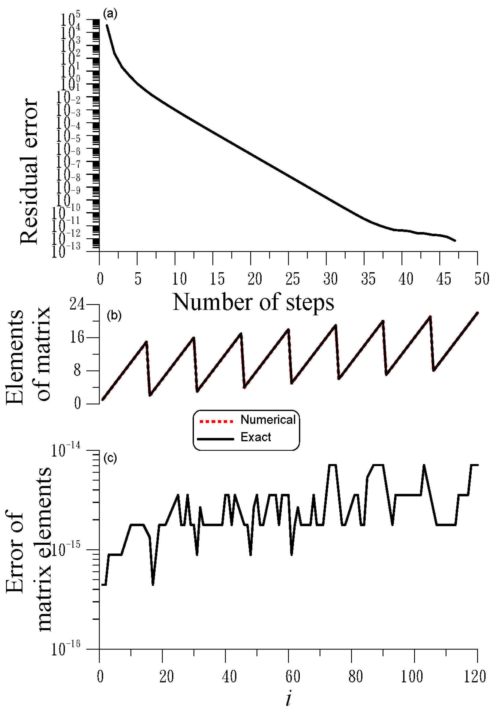
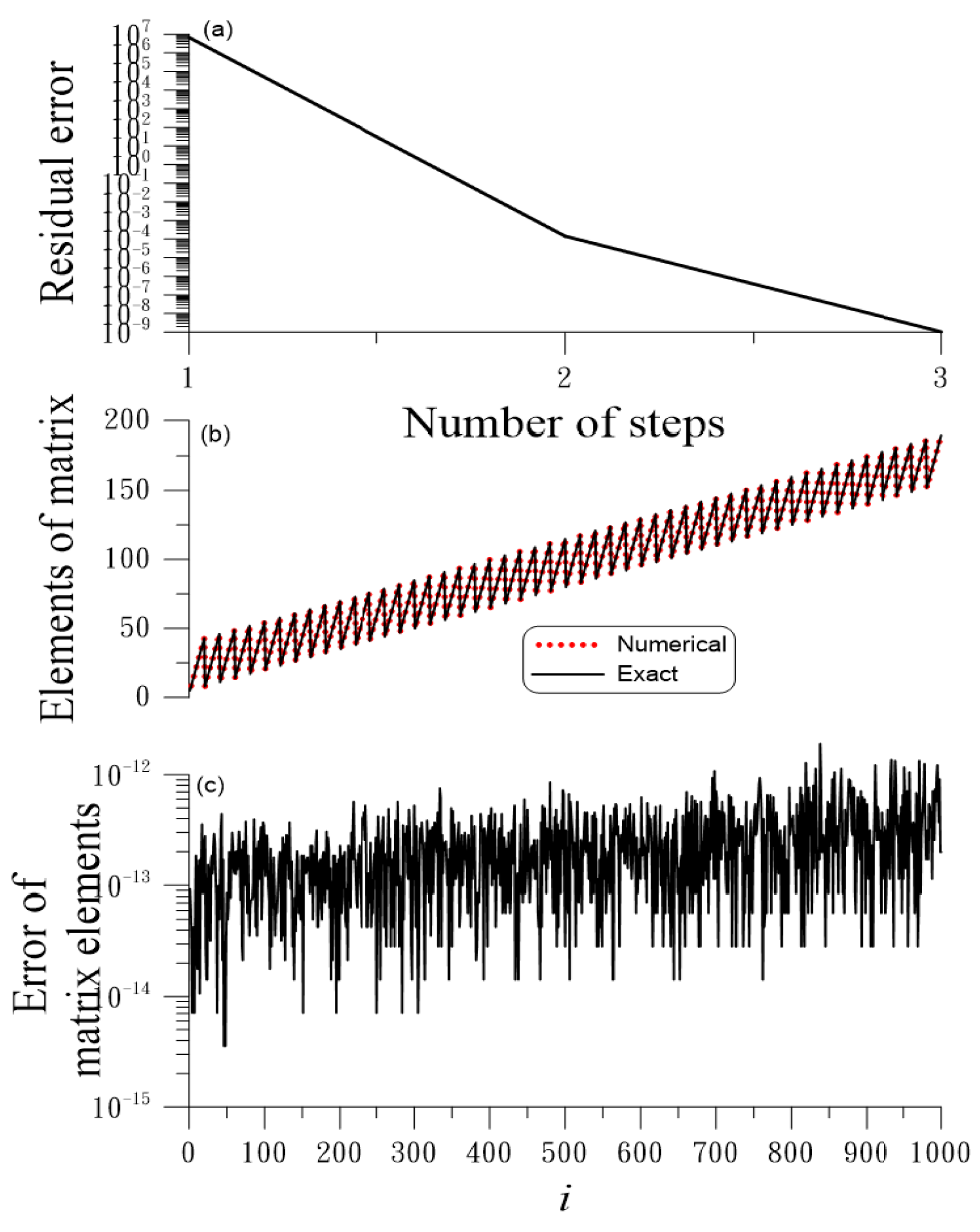
This problem belongs to Case 2. When we apply the iterative algorithm in Section 4 to find the solution, we fix $m=2$, and the convergence criterion is $\epsilon ={10}^{-12}$. As shown in Figure 2a, the DOIA converges very fast in 47 steps. As shown in Figure 2b, the numerical and exact solutions are almost coincident, with the numerical error shown in Figure 2c. The ME is $7.11\times {10}^{-15}$. Then, the DOIA(m), with $m_0=1$ and $m_1=2$, obtains an ME = $7.11\times {10}^{-15}$ in 43 steps.

Figure 2. For example 2 solved by the DOIA: (a) residual, (b) comparison of numerical and exact solutions, and (c) numerical error; (b,c) with the same x axis.

We consider the inverse matrix obtained in Case 2 with $q=p=n$ and $F=I_n$. Let X be the inverse matrix of A; the Newton–Schultz iterative method is

$$X_{k+1}=X_k(2I_n-A{X}_k).$$

For the initial value with $X_0=A^{\mathrm{T}}/{\parallel A\parallel }^2$, the Newton–Schultz iterative method can converge very quickly.

We consider the cyclic matrix constructed from Algorithm 3 for the cyclic matrix and apply the DOIA(m) to find the $A^{-1}$ with the same initial value with $X_0=A^{\mathrm{T}}/{\parallel A\parallel }^2$. Table 2 compares the $\parallel AX-I_n\parallel$ and iteration number (IN) obtained by the DOIA(m) and the Newton–Schultz iterative method (NSIM) with $\epsilon ={10}^{-15}$. The DOIA(m) can find a more accurate inverse matrix with a lower IN.

Table 2. For Example 2, ($\parallel AX-I_n\parallel$, IN) obtained by DOIA(m) and the Newton–Schultz iterative method (NSIM) for different n.

n	4	5	6	7
DOIA(m)	($3.82\times {10}^{-16}$, 4)	($4.60\times {10}^{-16}$, 4)	($8.37\times {10}^{-16}$, 7)	($8.12\times {10}^{-16}$, 14)
NSIM	($8.42\times {10}^{-16}$, 11)	($3.66\times {10}^{-16}$, 12)	($1.68\times {10}^{-16}$, 12)	($1.67\times {10}^{-15}$, 13)

For $n=7$, the CPU time of DOIA(m) is 0.41 s. Although n is raised to $n=50$, the DOIA(m), with $m_0=2$ and $m_1=3$, is still applicable, with $\parallel AX-I_n\parallel =7.72\times {10}^{-13}$ obtained in 149 steps, with a CPU time of 6.85 s.

5.3. Example 3

We consider

$$A=\left[\begin{array}{cccccc}1& 2& 3& 4& 5& 6\\ 2& 3& 4& 5& 6& 1\\ 3& 4& 5& 6& 1& 2\\ 4& 5& 6& 1& 2& 3\\ 5& 6& 1& 2& 3& 4\\ 6& 1& 2& 3& 4& 5\end{array}\right].$$

(133)

We first compute $A^{-1}$ and then the solution of the corresponding linear system. This problem belongs to Case 1.

We take $m=4$ and apply the DOS to find the inverse matrix of A by setting $B=I_6$ in Equation (11). The values of $AX-I_6$ obtained from the DOS with the accuracy to find the inverse matrix $A^{-1}$ has two orders. The residual error is $\parallel AX-I_5\parallel =0.159$. In the solution to Equation (4), when we compare the numerical solution with the exact solution $x_i=1,i=1,\dots ,6$, we find that the maximum error is $1.088\times {10}^{-4}$. Since the DOS is just a single-step DOIA, to improve the accuracy, we can apply the DOIA to solve the considered problem.

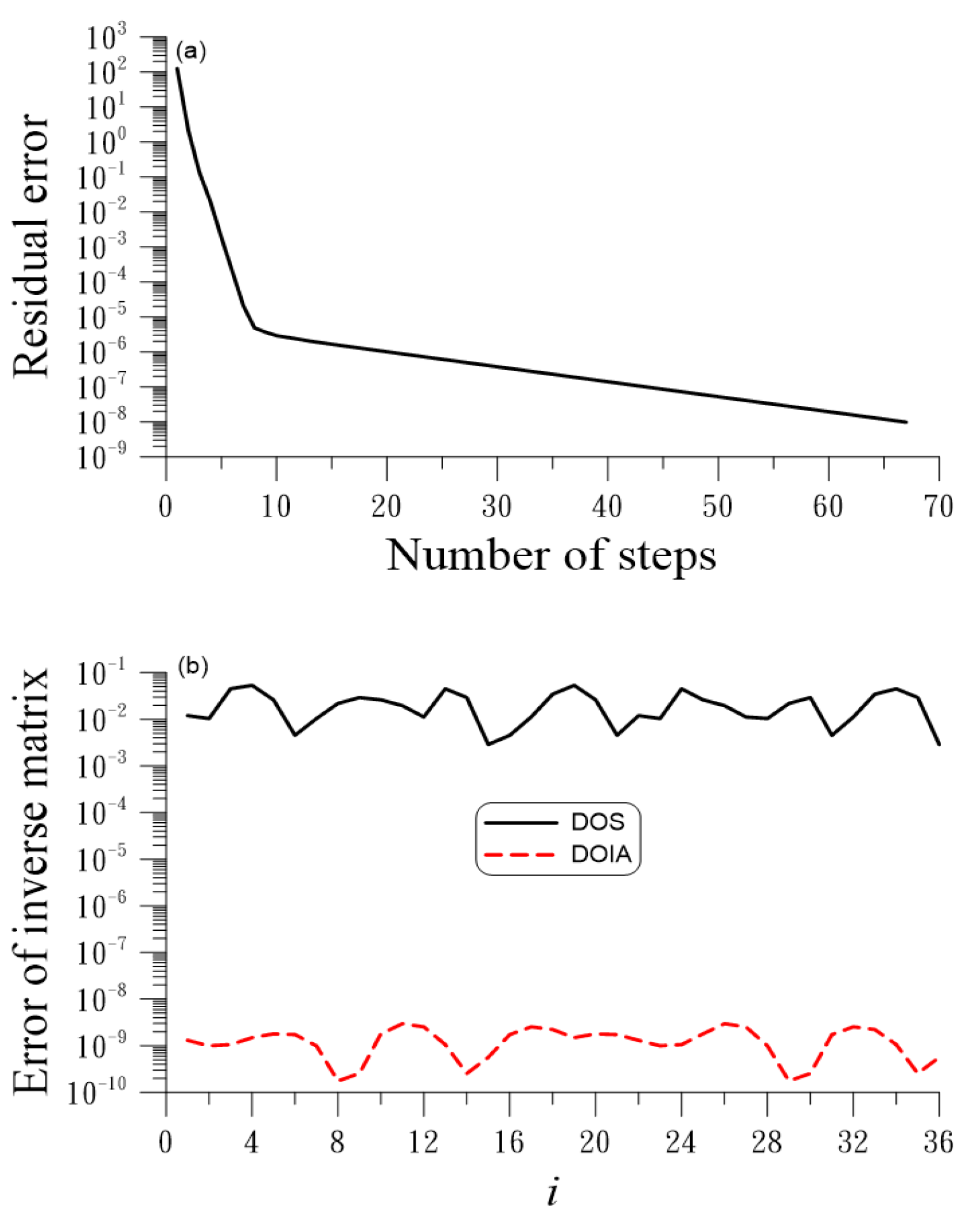
When we apply the DOIA to solve this problem with $m=3$, the accuracy can be raised to $\parallel AX-I_6\parallel =9.77\times {10}^{-9}$, while in the solution to Equation (4), ME = $5.73\times {10}^{-11}$. In Figure 3a, we show the residual error obtained by the DOIA, which is convergent in 67 steps under $\epsilon ={10}^{-8}$; Figure 3b compares the errors of the elements of the inverse matrix, using the components of $AX-I_6$. It can be seen that the DOIA is very effective and is much accurate than the DOS method. DOS is a single-step DOIA without iteration.

Figure 3. For example 3 solved by the DOS and DOIA, showing (a) residual and (b) comparison of error of inverse matrix.

For the DOIA(m) with $m_0=2$ and $m_1=4$, it converges in 28 steps under $\epsilon ={10}^{-8}$; the accuracy can be raised to $\parallel AX-I_6\parallel =9.73\times {10}^{-9}$, and ME = $2.13\times {10}^{-11}$. The CPU time of the DOIA(m) is 0.33 s, which converges faster than the DOIA.

To test the stability of the DOIA, we consider random noise with intensity s to disturb the coefficients in Equation (133). We take the same values of the parameters in the DOIA. Table 3 compares $\parallel AX-I_6\parallel$, ME, and iteration number (IN). Essentially, the noise does not influence the accuracy of $\parallel AX-I_6\parallel$; however, ME and IN worsen when s increases.

Table 3. For Example 3, $\parallel AX-I_6\parallel$, ME, and IN obtained by DOIA for different noise s values.

s	0	0.01	0.03	0.05	0.1
$\parallel AX-I_6\parallel$	$9.77\times {10}^{-9}$	$9.74\times {10}^{-9}$	$9.61\times {10}^{-9}$	$9.82\times {10}^{-9}$	$9.96\times {10}^{-9}$
ME	$5.73\times {10}^{-11}$	$8.24\times {10}^{-3}$	$2.48\times {10}^{-2}$	$4.15\times {10}^{-2}$	$8.37\times {10}^{-2}$
IN	67	124	84	246	622

5.4. Example 4

By testing the performance of the DOS on the solution to the linear equation system, we consider the following convex quadratic programming problem with an equality constraint:

$$\begin{array}{ccc}\hfill & & min\left\{f=\frac{1}{2}{x}^{\mathrm{T}}Px+q^{\mathrm{T}}x\right\},\hfill \end{array}$$

(134)

$$\begin{array}{ccc}\hfill & & Cx=b_0,\hfill \end{array}$$

(135)

where P is an $n_1\times n_1$ matrix, C is an $m_1\times n_1$ matrix, and $b_0$ is an $m_1$ vector, which means that Equation (135) provides $m_1$ linear constraints. According to Lagrange theory, we need to solve the linear system (4) with the following b and A:

$$\begin{array}{ccc}\hfill & & b:=\left[\begin{array}{c}-q\\ b_0\end{array}\right],\hfill \\ & & A=\left[\begin{array}{cc}P& C^{\mathrm{T}}\\ C& 0_{m_1\times m_1}\end{array}\right].\hfill \end{array}$$

For a definite solution, we take $n_1=3$ and $m_1=2$ with

$$\begin{array}{ccc}\hfill & & min\{f=x_1^2+2x_2^2+x_3^2-2x_1{x}_2+x_3\},\hfill \\ & & x_1+x_2+x_3=4,\hfill \\ & & 2x_1-x_2+x_3=2.\hfill \end{array}$$

The dimension of A is $n\times n$, where $n=n_1+m_1=5$. This problem belongs to Case 1. When we take $m=4$ and employ the DOS, ${\lambda }_0=-0.3716283$ and ${\alpha }_0=-2.690861$ meet ${\alpha }_0{\lambda }_0=1$. With $x=A^{-1}b$, the solution is $minf=3.977273$ at $(x_1,x_2,x_3)=(1.909091,1.954545,0.136364)$ with $\parallel Ax-b\parallel =3.729\times {10}^{-15}$; it is almost an exact solution obtained without any iteration, because the DOS can be viewed as a single-step DOIA.

5.5. Example 5: Solving Ill-Conditioned Hilbert Matrix Equation

The Hilbert matrix is highly ill-conditioned:

$$A_{ij}=\frac{1}{i+j-1}.$$

(136)

We consider an exact solution with $x_j=1,j=1,\dots ,n$, and $b_i$ is given by

$$b_i=\sum _{j=1}^n\frac{1}{i+j-1}.$$

It is known that the Hilbert matrix is a highly ill-conditioned matrix. For $n=5$, the condition number is $4.81\times {10}^5$, and, for $n=10$, the condition number is $1.19\times {10}^9$. It can be proved that the asymptotic of the condition number of the Hilbert matrix is [50]

$$\mathcal{O}\left(\frac{{(1+\sqrt{2})}^{4n+4}}{\sqrt{n}}\right).$$

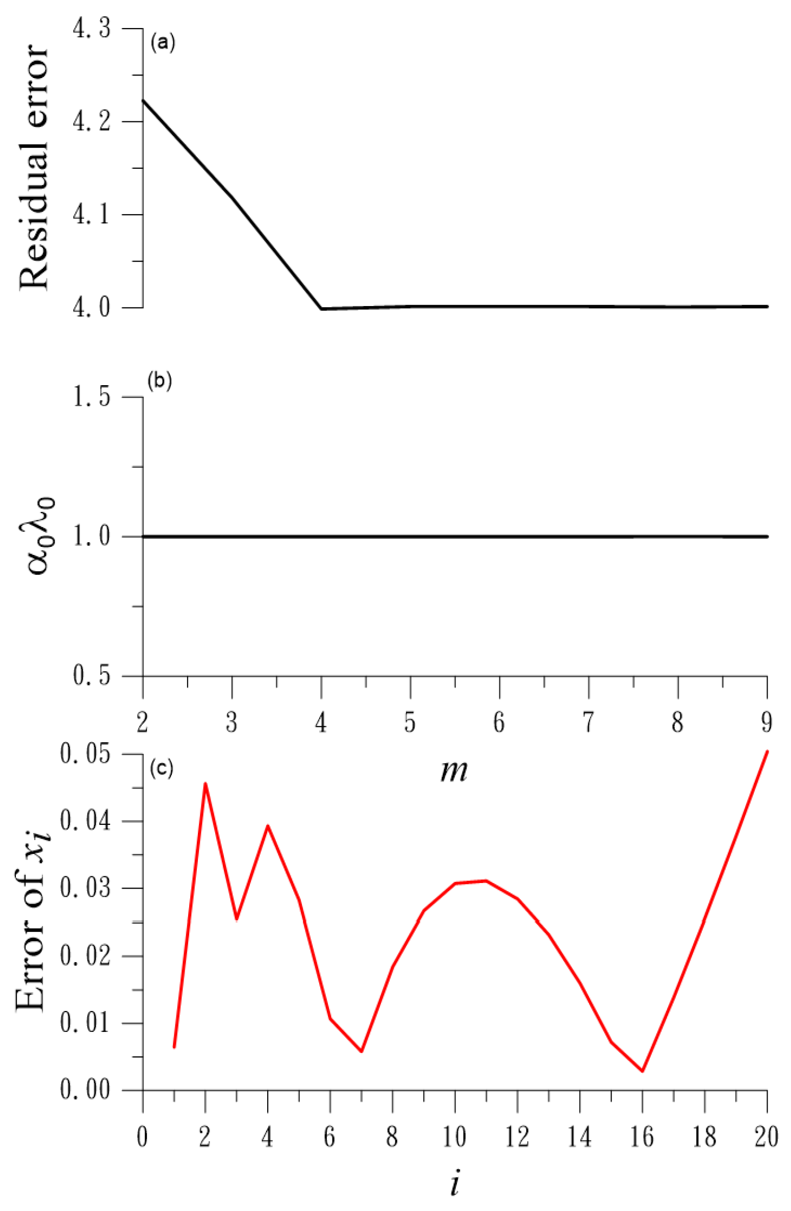
This problem belongs to Case 1. We solve this problem by using the DOS. For $n=20$, we let m run from 2 to 9, and peak the best m with the minimum error of

$$\parallel AX-I_n\parallel .$$

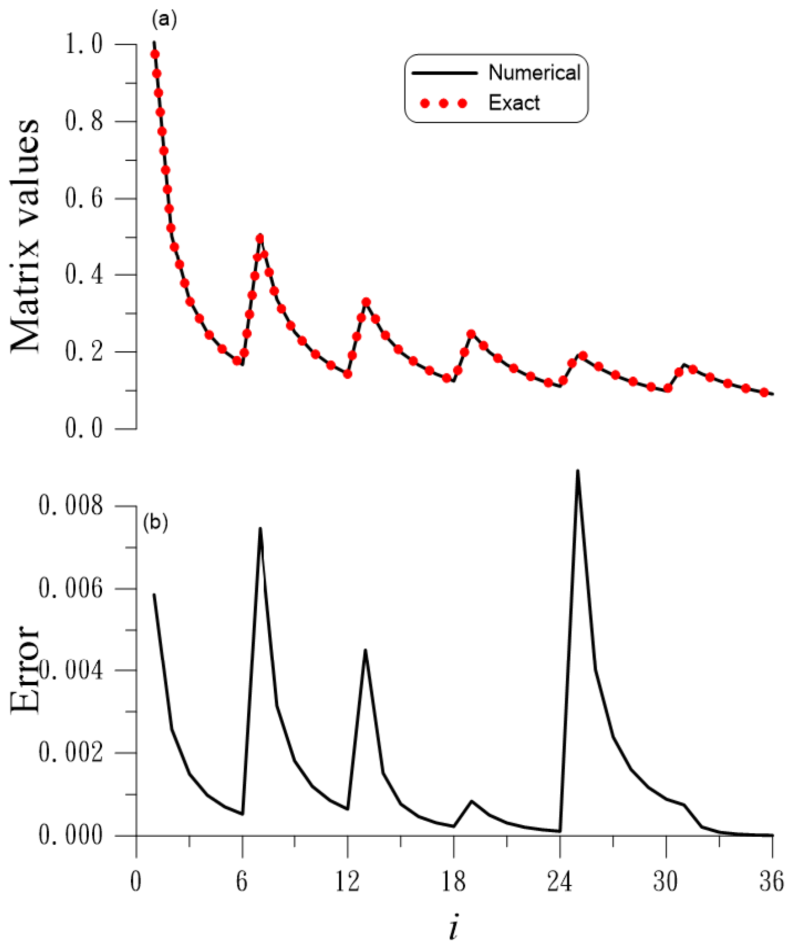
In Figure 4a, we plot the above residual with respect to m, where we can observe that the value of ${\alpha }_0{\lambda }_0$ is almost equal to 1, as shown in Figure 4b. We take $m=4$, and the maximum error of x is $0.05$.

Figure 4. For Example 5 solved by the DOS, showing (a) residual, (b) ${\alpha }_0{\lambda }_0$, and (c) error of $x_i$; (a,b) the same x axis.

Below, we solve the inverse of a five-dimensional Hilbert matrix with $n=5$ by using the DOS method, where we take $m=3$. It is interesting that $X=A^{-1}$ is also symmetric. The residual error is $\parallel AX-I_5\parallel =1.443$. However, when we apply the DOIA to solve this problem with $m=3$, the accuracy of $\parallel AX-I_5\parallel$ can be raised to $\parallel AX-I_5\parallel =0.912$. In Figure 5a, we show the residual error obtained by the DOIA, which does not converge within 100 steps under $\epsilon ={10}^{-8}$. Figure 5b compares the error of the elements of the inverse matrix by using the components of $AX-I_5$. Due to the highly ill-conditioned nature of the Hilbert matrix, the results obtained by the DOS and DOIA are quite different. ME = $1.51\times {10}^{-2}$ is obtained for $x_i$.

Figure 5. For Example 5 solved by the DOS, DOIA, and DOIA(m), showing (a) residuals, (b) comparing error of inverse matrix.

For the DOIA(m) with $m_0=2$ and $m_1=4$, it converges in 62 steps under $\epsilon ={10}^{-8}$; the accuracy can be raised to $\parallel AX-I_5\parallel =6.83\times {10}^{-9}$, and ME = $1.48\times {10}^{-9}$. Obviously, the DOIA(m) can significantly improve the convergence speed and accuracy.

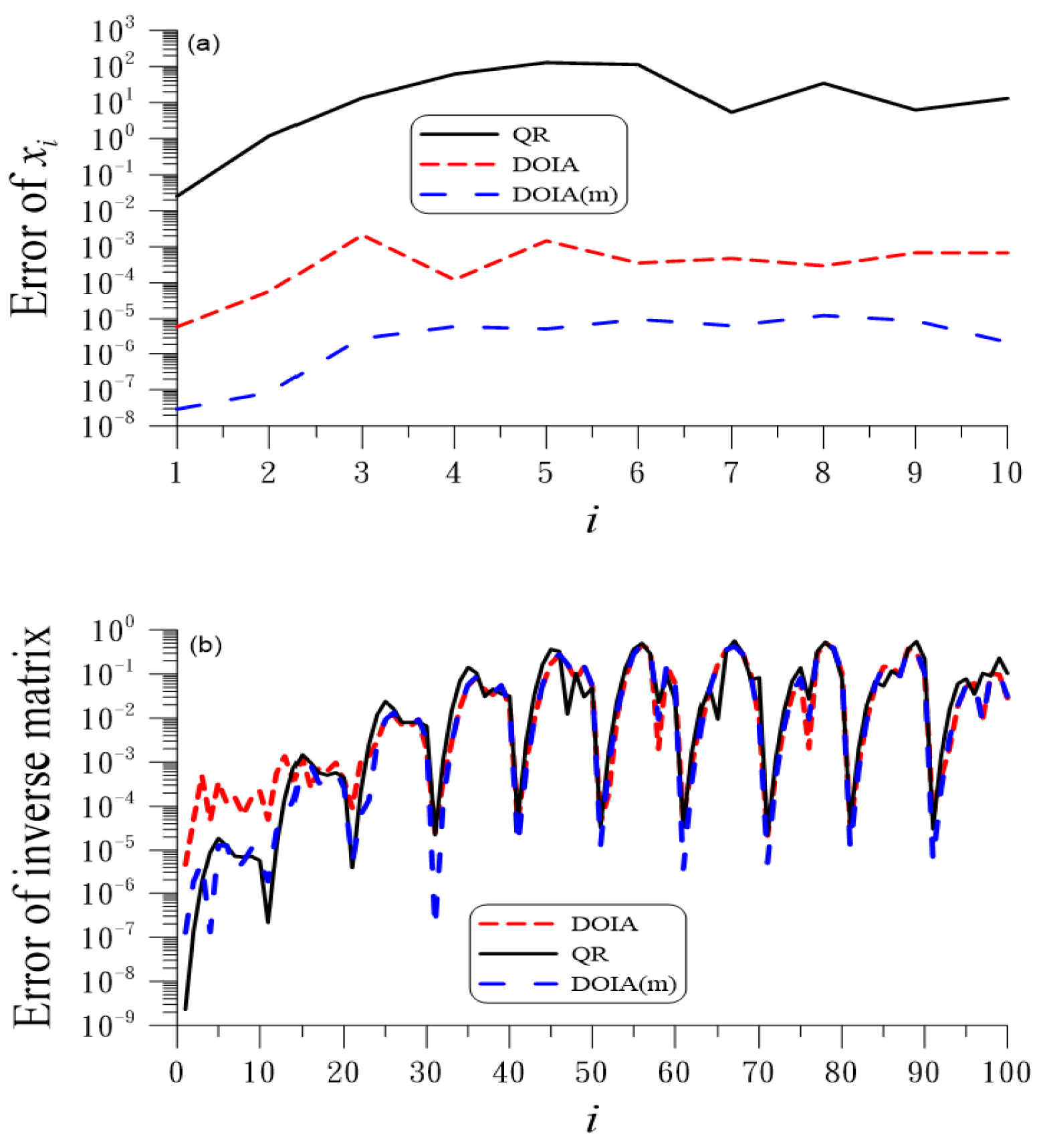
Then, we compare the numerical results with those obtained with the QR method. For $n=10$, we apply the DOIA to solve this problem with $m=7$, and the accuracy is $\parallel AX-I_{10}\parallel =1.371$, while that obtained with the QR method is $\parallel AX-I_{10}\parallel =1.574$. In Figure 6a, we compare the solutions of linear system (4), where the exact solution is supposed to be $x_i=1,i=1,\dots ,10$. Whereas the DOIA provides quite accurate solutions with ME = $2.117\times {10}^{-3}$, the QR method fails, as the diagonal elements of matrix R are very small for the ill-conditioned Hilbert matrix. The errors of the inverse matrix obtained with these two methods are comparable, as shown in Figure 6b.

Figure 6. For example 5 solved by the DOIA, DOIA(m), and QR, comparing errors of (a) $x_i$, and (b) inverse matrix.

The DOIA(m) with $m_0=2$ and $m_1=6$ does not converge within 100 steps under $\epsilon ={10}^{-8}$; however, the accuracy can be raised to ME = $1.24\times {10}^{-5}$.

We consider the Hilbert matrix in Equation (136) and apply the DOIA(m) to find $A^{-1}$ with an initial value $X_0=A^{\mathrm{T}}/{\parallel A\parallel }^2$. Because the Newton–Schultz iterative method (NSIM) converges slowly, we give the upper bound IN = 500. Table 4 compares the $\parallel AX-I_n\parallel$ and IN obtained with the DOIA(m) with $\epsilon ={10}^{-10}$ and NSIM. DOIA(m) can find an accurate inverse matrix in fewer interations.

Table 4. For Example 5, the $\parallel AX-I_n\parallel$ and IN obtained by DOIA(m) and the Newton–Schultz iterative method (NSIM) for different n.

n	4	5	6
DOIA(m)	($1.41\times {10}^{-13}$, 5)	($9.70\times {10}^{-12}$, 9)	($8.92\times {10}^{-10}$, 148)
NSIM	($3.27\times {10}^{-13}$, 500)	($4.81\times {10}^{-12}$, 500)	($1.80\times {10}^{-10}$, 500)

5.6. Example 6

In this example, we apply the DOS with $m=5$ to solve a six-dimensional matrix Equation (11) with the coefficient matrix A given in Equation (133), and the solution is the Hilbert matrix given in Equation (136) with $n=6$. First, we find the right inversion of A from $AX=I_6$ by using the DOS, and then the solution of the matrix equation is given by $X^{\mathrm{T}}B$. The numerical solution of the matrix elements with $i=1,\dots ,36$, which is obtained by arranging the matrix element from left to right and top to bottom with a consecutive Arabic number, is compared with the exact one in Figure 7a; the numerical error is shown in Figure 7b, which is smaller than 0.008. The residual error $\parallel AX-B\parallel$ is 0.0157, which is quite accurate.

Figure 7. For example 6 solved by the DOS: (a) comparing numerical and exact solutions, (b) numerical error of matrix elements; (a,b) with the same x axis.

For the DOIA(m) with $m_0=1$ and $m_1=2$, it converges in 28 steps under $\epsilon ={10}^{-10}$; the accuracy raises to $\parallel AX-B\parallel =1.47\times {10}^{-11}$, and ME = $9.24\times {10}^{-13}$. The convergence can be accelerated to 14 steps when we take $m_0=1$ and $m_1=5$; the accuracy is slightly decreased to ME = $4.35\times {10}^{-12}$ and $\parallel AX-B\parallel =4.96\times {10}^{-11}$.

5.7. Example 7

Consider the mixed boundary value problem of the Laplace equation:

$$\begin{array}{ccc}\hfill & & \mathrm{\Delta }u=u_{rr}+\frac{1}{r}{u}_r+\frac{1}{r^2}{u}_{\theta \theta }=0,\hfill \\ \hfill & & u(\rho ,\theta )=h\left(\theta \right),0\le \theta \le \pi ,\hfill \\ \hfill & & u_n(\rho ,\theta )=g\left(\theta \right),\pi \le \theta \le 2\pi .\hfill \end{array}$$

The method of fundamental solutions is taken as

$$u\left(\mathbf{x}\right)=\sum _{j=1}^n{c}_{j}U(\mathbf{x},{\mathbf{s}}_j),{\mathbf{s}}_j\in {\mathrm{\Omega }}^c.$$

where

$$U(\mathbf{x},{\mathbf{s}}_j)=ln{r}_j,r_j=\parallel \mathbf{x}-{\mathbf{s}}_j\parallel .$$

We consider

$$\begin{array}{ccc}\hfill & & u(x,y)=\cos xcoshy+\sin xsinhy,\hfill \\ \hfill & & \rho \left(\theta \right)=exp\left(\sin \theta \right){\sin }^2\left(2\theta \right)+exp\left(\cos \theta \right){\cos }^2\left(2\theta \right).\hfill \end{array}$$

This problem is a special Case 2 with $p=1$. We take $q=50$ and $n=30$. ME = $3.19\times {10}^{-2}$ is obtained in 174 steps by the DOIA(m) with $m_0=4$ and $m_1=5$. The CPU time is 0.65 s. It can also be treated as a special Case 1 with $p=1$. We take $n=50$. ME = $5.5\times {10}^{-2}$ is obtained within 300 steps by the DOIA(m) with $m_0=2$ and $m_1=3$. The CPU time is 0.62 s. To improve the accuracy, we can develop the vector form of the DOIA(m), which is, however, another issue not reported here.

According to [6], we apply the GMRES(m) with $m=50$ to solve this problem. ME = $4.8\times {10}^{-2}$ is obtained in 2250 steps, and the CPU time is 2.19 s.

6. Pseudoinverse of Rectangular Matrix

The Moore–Penrose pseudoinverse of A denoted as $A^{†}$ is the most famous for the inversion of a rectangular matrix, satisfying the following Penrose equations:

$$\begin{array}{ccc}\hfill & & A{A}^{†}A=A,\hfill \end{array}$$

(137)

$$\begin{array}{ccc}\hfill & & A^{†}A{A}^{†}=A^{†},\hfill \end{array}$$

(138)

$$\begin{array}{ccc}\hfill & & {\left(A{A}^{†}\right)}^{\mathrm{T}}=A{A}^{†},\hfill \end{array}$$

(139)

$$\begin{array}{ccc}\hfill & & {\left(A^{†}A\right)}^{\mathrm{T}}=A^{†}A.\hfill \end{array}$$

(140)

6.1. A New Matrix Pencil

We rewrite Equation (8) as

$$AX=I_q;$$

(141)

upon giving an initial value $X_0$, we attempt to seek the next step solution X with

$$X={\alpha }_0{X}_0+\sum _{k=1}^m{\alpha }_k{U}_k,$$

(142)

where $U_k=X_0{\left(A{X}_0\right)}^k$. The new matrix pencil with degree m is given by

$$\mathcal{U}=[U_1,\dots ,U_m]=[X_{0}A{X}_0,\dots ,X_0{\left(A{X}_0\right)}^m],$$

(143)

which consists of an m-degree polynomial of $A{X}_0$. The modified Gram–Schmidt process is employed to orthogonalize and normalize $\mathcal{U}$.

The iterative form of Equation (142) is

$$X_{k+1}={\alpha }_0^k{X}_k+{\alpha }_1^k{X}_{k}A{X}_k+{\alpha }_2^k{X}_k{\left(A{X}_k\right)}^2+\dots +{\alpha }_m^k{X}_k{\left(A{X}_k\right)}^m.$$

(144)

Notice that it includes several iterative algorithms as special cases: the Newton–Schultz method [30], the Chebyshev method [31], the Homeier method [32], the PS method (PSM) by Petkovic and Stanimirovic [38], and the KKRJ [36]:

$$\begin{array}{ccc}\hfill & & X_{k+1}=2X_k-X_{k}A{X}_k(\mathrm{Newton}–\mathrm{Schultz} \mathrm{method}),\hfill \end{array}$$

(145)

$$\begin{array}{ccc}\hfill & & X_{k+1}=3X_k-3X_{k}A{X}_k+X_k{\left(A{X}_k\right)}^2(\mathrm{Chebyshev} \mathrm{method}),\hfill \end{array}$$

(146)

$$\begin{array}{ccc}\hfill & & X_{k+1}=\frac{7}{2}{X}_k-\frac{9}{2}{X}_{k}A{X}_k+\frac{5}{2}{X}_k{\left(A{X}_k\right)}^2-\frac{1}{2}{X}_k{\left(A{X}_k\right)}^3(\mathrm{Homeier} \mathrm{method}),\hfill \end{array}$$

(147)

$$\begin{array}{ccc}\hfill & & X_{k+1}=(1+\beta )X_k-\beta X_{k}A{X}_k,(\mathrm{PS} \mathrm{method}),\hfill \end{array}$$

(148)

$$\begin{array}{ccc}\hfill & & X_{k+1}=(3+\beta )X_k-(3+3\beta )X_{k}A{X}_k+(1+3\beta )X_k{\left(A{X}_k\right)}^2\hfill \\ & & -\beta X_k{\left(A{X}_k\right)}^3(\mathrm{KKRJ} \mathrm{method}).\hfill \end{array}$$

(149)

In Equation (144), two optimization methods are used to determine the coefficients ${\alpha }_0^k,{\alpha }_1^k,\dots ,{\alpha }_m^k$.

The results in Theorem 1 are also applicable to problem (141). Hence, we propose the following iterative algorithm, namely, the Moore–Penrose iterative algorithm (MPIA).

MPIA is a new algorithm based on the newly developed DOIA in Section 4; MPIA is used as a new matrix pencil in Equation (143) and with $U_0=X_0$. The motivation for the development of MPIA using $U_k=X_0{\left(A{X}_0\right)}^k$ in the matrix pencil is that we can generalize the methods in Equations (145)–(149) to the m orders method and provide a theoretical foundation to determine the expansion coefficients from the double-optimization technique (Algorithm 4).

Algorithm 4 MPIA

1: Select m and give $X_0$ 2: Do $k=0,1,\dots$ 3:    $U_j^k=X_k{\left(A{X}_k\right)}^j,j=1,\dots ,m$ 4:    ${\mathcal{U}}_k=[U_1^k,\dots ,U_m^k]$ (orthonormalization) 5:    ${\mathcal{Y}}_k=[Y_1^k,\dots ,Y_m^k]=[A{U}_1^k,\dots ,A{U}_m^k]$ 6:    $C_{ij}^k=Y_i^k:Y_j^k,C_k=\left[C_{ij}^k\right]$ 7:    $D_k=C_k^{-1}$ 8:    $v_i^k=I_q:Y_i^k,v_k=\left[v_i^k\right]$ 9:    $u_i^k=\left(A{X}_k\right):Y_i^k,u_k=\left[u_i^k\right]$ 10:   ${\lambda }_k=\frac{\parallel A{X}_k{\parallel }^2-u_k^{\mathrm{T}}{D}_k{u}_k}{I_q:\left(A{X}_k\right)-v_k^{\mathrm{T}}{D}_k{u}_k}$ 11:   $W_k={\lambda }_k{\mathcal{Y}}_k{D}_k{v}_k+A{X}_k-{\mathcal{Y}}_k{D}_k{u}_k$ 12:   ${\alpha }_k=\frac{I_q:W_k}{\parallel W_k{\parallel }^2}$ 13:   $X_{k+1}={\alpha }_k[X_k+{\lambda }_k{\mathcal{U}}_k{D}_k{v}_k-{\mathcal{U}}_k{D}_k{u}_k]$ 14: Enddo, if $\parallel X_{k+1}-X_k\parallel <\epsilon$

Like DOIA(m), the MPIA(m) can be constructed similarly.

6.2. Optimized Hyperpower Method

Pan et al. [51] proposed the following hyperpower method:

$$X_{k+1}=X_k\sum _{i=0}^{p-1}{(I_q-A{X}_k)}^i;$$

(150)

also refer to [52,53]. Equation (150) includes the Newton–Schultz method [30], and the Chebyshev method [31] as special cases.

Let $m=p-1$, and Equation (150) is rewritten as

$$X_{k+1}=X_k+\sum _{i=1}^m{(I_q-A{X}_k)}^i;$$

(151)

we generalize it to

$$X_{k+1}={\alpha }_0^k{X}_k+\sum _{i=1}^m{\alpha }_i^k{(I_q-A{X}_k)}^i.$$

(152)

Equation (152) is used to find the optimized descent matrix X in the current-step residual equation:

$$AX=R_k=I_q-A{Z}_k.$$

(153)

Two optimization methods are used to determine the coefficients ${\alpha }_0^k,{\alpha }_1^k,\dots ,{\alpha }_m^k$. The results in Theorem 1 are also applicable to problem (153). Hence, we propose the following iterative algorithm, namely, the optimized hyperpower iterative algorithm (OHPIA(m)); we take the restarted technique into consideration. Since the matrix pencil consists of the powers of the residual matrices, the orthonormalization for ${\mathcal{U}}_k$ is not suggested (Algorithm 5).

Algorithm 5 OHPIA(m)

1: Select $m_0$ and $m_1$, and give $Z_0$ 2: Do $i=1,\dots$ 3: Do $m=m_0,\dots ,m_1$, $k=m-m_0$ 4:    $U_0^k=X_k$ 5:    $U_j^k=X_k{R}_k^j=X_k{(I_q-A{Z}_k)}^j,j=1,\dots ,m$ 6:    ${\mathcal{U}}_k=[U_1^k,\dots ,U_m^k]$ 7:    ${\mathcal{Y}}_k=A{\mathcal{U}}_k$ 8:    $C_{ij}^k=Y_i^k:Y_j^k,C_k=\left[C_{ij}^k\right]$ 9:    $D_k=C_k^{-1}$ 10:   $v_i^k=R_k:Y_i^k,v_k=\left[v_i^k\right]$ 11:   $u_i^k=\left(A{U}_0^k\right):Y_i^k,u_k=\left[u_i^k\right]$ 12:   ${\lambda }_k=\frac{\parallel A{U}_0^k{\parallel }^2-u_k^{\mathrm{T}}{D}_k{u}_k}{R_k:\left(A{U}_0^k\right)-v_k^{\mathrm{T}}{D}_k{u}_k}$ 13:   $W_k={\lambda }_k{\mathcal{Y}}_k{D}_k{v}_k+A{U}_0^k-{\mathcal{Y}}_k{D}_k{u}_k$ 14:   ${\alpha }_k=\frac{R_k:W_k}{\parallel W_k{\parallel }^2}$ 15:   $X_k={\alpha }_k[U_0^k+{\lambda }_k{\mathcal{U}}_k{D}_k{v}_k-{\mathcal{U}}_k{D}_k{u}_k]$ 16:   $Z_{k+1}=Z_k+X_k$ 17: Enddo of (3), if $\parallel R_{k+1}\parallel <\epsilon$ 18: Otherwise, $Z_0=Z_{k+1}$, go to (2)

OHPIA is a new algorithm based on the DOIA newly developed in Section 4; OHPIA is used a new matrix pencil derived from Equation (152):

$$\mathcal{U}=[U_1,\dots ,U_m]=[I_q-A{X}_k,\dots ,{(I_q-A{X}_k)}^m].$$

7. Numerical Testing of Rectangular Matrix

7.1. Example 8

We find the Moore–Penrose inverse of the following rank-deficient matrix [54]:

$$A=\left[\begin{array}{cccc}-1& 0& 1& 2\\ -1& 1& 0& -1\\ 0& -1& 1& 3\\ 0& 1& -1& -3\\ 1& -1& 0& 1\\ 1& 0& -1& -2\end{array}\right].$$

This problem belongs to Case 2. We apply the iterative method of the DOIA to find the Moore–Penrose inverse, which has an exact solution:

$$A^{†}=\frac{1}{102}\left[\begin{array}{cccccc}-15& -18& 3& -3& 18& 15\\ 8& 13& -5& 5& -13& -8\\ 7& 5& 2& -2& -5& -7\\ 6& -3& 9& -9& 3& -6\end{array}\right].$$

(154)

Under the same convergence criterion $\epsilon ={10}^{-9}$ as used by Xia et al. [54], the iteration process of the DOIA with $m=1$ converges very fast in three steps. By comparison to Equation (154), ME = $7.3\times {10}^{-9}$ is obtained.

In Table 5, we compare the DOIA ($m=1$ and $\epsilon ={10}^{-15}$) with other numerical methods specified by Xia et al. [54], Petkovic and Stanimirovic [38], and Kansal et al. [36], to asses the performance of the DOIA measured using four numerical errors of the Penrose equations (137)–(140) and the iteration number (IN).

Table 5. Computed results of a rank-deficient matrix in Example 8.

Alg.	IP	$\parallel {\mathit{AA}}^{†}{\mathit{A}-\mathit{A}\parallel }^2$	$\parallel {\mathit{A}}^{†}{\mathit{AA}}^{†}-{\mathit{A}}^{†}{\parallel }^2$	$\parallel {\left({\mathit{AA}}^{†}\right)}^{\mathbf{T}}-{\mathit{AA}}^{†}{\parallel }^2$	$\parallel {\left({\mathit{A}}^{†}\mathit{A}\right)}^{\mathbf{T}}-{\mathit{A}}^{†}{\mathit{A}\parallel }^2$	IN
[54]	${10}^{-5}{A}^{\mathrm{T}}$	$8.92\times {10}^{-16}$	$3.36\times {10}^{-16}$	$7.85\times {10}^{-17}$	$1.97\times {10}^{-15}$	50
[54]	$0.1A^{\mathrm{T}}$	$9.17\times {10}^{-20}$	$6.99\times {10}^{-16}$	$7.85\times {10}^{-17}$	$2.86\times {10}^{-15}$	60
PSM	$0.1A^{\mathrm{T}}$	$1.53\times {10}^{-14}$	$9.21\times {10}^{-17}$	$4.13\times {10}^{-31}$	$1.17\times {10}^{-30}$	165
KKRJ	$0.025A^{\mathrm{T}}$	$3.01\times {10}^{-30}$	$2.25\times {10}^{-29}$	$2.28\times {10}^{-31}$	$1.53\times {10}^{-30}$	6
NSIM	$A^{\mathrm{T}}/{\parallel A\parallel }^2$	$4.01\times {10}^{-31}$	$2.60\times {10}^{-31}$	$1.29\times {10}^{-31}$	$2.20\times {10}^{-32}$	9
DOIA	$X_0=0$	$2.80\times {10}^{-31}$	$4.83\times {10}^{-33}$	$6.16\times {10}^{-33}$	$1.78\times {10}^{-32}$	3

Recently, Kansal et al. [36] proposed the iterative scheme in Equation (149). For this problem, we take $\beta =0.5$. When we take $\epsilon ={10}^{-15}$, it overflows; hence, we take $\epsilon ={10}^{-13}$.

In the above, Alg. is the abbreviation for Algorithm, IP represents the initial point, and IN is the iteration number. $\mathbf{1}={(1,\dots ,1)}^{\mathrm{T}}$. The first two algorithms were reported by Xia et al. [54]. It can be seen that the DOIA converges much faster and is more accurate than theother algorithms.

In the computation of the pseudoinverse, the last two singular values close to zero can be prevented from appearing in the matrix $\mathbf{C}\in {\mathbb{R}}^{m\times m}$ if m is small enough. For example, we take $m=1$ in Table 5, such that $D=C^{-1}$ can be computed accurately without being induced by the zero singular value appearing in the denominator to enlarge the rounding error.

7.2. Example 9: Inverting the Ill-Conditioned Rectangular Hilbert Matrix

We want to find the Moore–Penrose inverse of the Hilbert matrix:

$$A_{ij}=\frac{1}{i+j-1},1\le i\le q,1\le j\le n.$$

This problem belongs to Case 2. This is more difficult than the previous example. Here, we fix $q=50$, $n=3$. The numerical errors of the Penrose Equations (137)–(140) are compared in Table 6. In the DOIA(m) and OHPIA(m), we take $m_0=1$, $m_1=2$ and $\epsilon ={10}^{-10}$. DOIA(m) and OHPIA(m) converge faster than in [36,38].

Table 6. Computed results of the Hilbert matrix with $q=50$, $n=3$ in Example 9.

Alg.	IP	$\parallel {\mathit{AA}}^{†}{\mathit{A}-\mathit{A}\parallel }^2$	$\parallel {\mathit{A}}^{†}{\mathit{AA}}^{†}-{\mathit{A}}^{†}{\parallel }^2$	$\parallel {\left({\mathit{AA}}^{†}\right)}^{\mathbf{T}}-{\mathit{AA}}^{†}{\parallel }^2$	$\parallel {\left({\mathit{A}}^{†}\mathit{A}\right)}^{\mathbf{T}}-{\mathit{A}}^{†}{\mathit{A}\parallel }^2$	IN
PSM	$0.8A^{\mathrm{T}}$	$1.4\times {10}^{-28}$	$3.7\times {10}^{-21}$	$4.1\times {10}^{-30}$	$3.5\times {10}^{-27}$	34
KKRJ	$0.38A^{\mathrm{T}}$	$1.01\times {10}^{-28}$	$9.45\times {10}^{-27}$	$2.52\times {10}^{-26}$	$5.77\times {10}^{-27}$	12
NSIM	$A^{\mathrm{T}}/{\parallel A\parallel }^2$	$5.65\times {10}^{-29}$	$1.40\times {10}^{-26}$	$1.69\times {10}^{-27}$	$2.60\times {10}^{-27}$	20
DOIA(m)	$X=0_{n\times q}$	$1.35\times {10}^{-29}$	$1.99\times {10}^{-25}$	$1.54\times {10}^{-26}$	$7.32\times {10}^{-27}$	3
OHPIA(m)	$A^{\mathrm{T}}/{\parallel A\parallel }^2$	$1.61\times {10}^{-29}$	$7.52\times {10}^{-26}$	$2.23\times {10}^{-26}$	$9.58\times {10}^{-28}$	3

Next, we find the Moore–Penrose inverse of the Hilbert matrix with $n=10$ and $q=15$. For MPIA, $m=3$; $(m_0,m_1)=(1,6)$ for MPIA(m). For the method in [36], which does not converge with $\epsilon ={10}^{-6}$, it is not applicable to find the inverse of a highly ill-conditioned Hilbert matrix with $q=15$ and $n=10$ (Table 7). Like the KKRJ, the OHPIA(m) is weak for highly ill-conditioned Hilbert matrices; the errors of $\parallel A^{†}A{A}^{†}-A^{†}{\parallel }^2$ and $\parallel {\left(A^{†}A\right)}^{\mathrm{T}}-A^{†}{A\parallel }^2$ raise to the order of ${10}^{11}$.

Table 7. Computed results of the Hilbert matrix with $q=15$ and $n=10$.

Alg.	IP	$\parallel {\mathit{AA}}^{†}{\mathit{A}-\mathit{A}\parallel }^2$	$\parallel {\mathit{A}}^{†}{\mathit{AA}}^{†}-{\mathit{A}}^{†}{\parallel }^2$	$\parallel {\left({\mathit{AA}}^{†}\right)}^{\mathbf{T}}-{\mathit{AA}}^{†}{\parallel }^2$	$\parallel {\left({\mathit{A}}^{†}\mathit{A}\right)}^{\mathbf{T}}-{\mathit{A}}^{†}{\mathit{A}\parallel }^2$	IN
RRKJ	$A^{\mathrm{T}}/{\parallel A\parallel }^2$	$2.58\times {10}^{-9}$	$1.44\times {10}^{12}$	$1.17\times {10}^{-6}$	$2.78\times {10}^{11}$	>500
MPIA	$A^{\mathrm{T}}/{\parallel A\parallel }^2$	$2.34\times {10}^{-6}$	$2.84\times {10}^{-2}$	$1.49\times {10}^{-3}$	$8.66\times {10}^{-4}$	50
MPIA(m)	$A^{\mathrm{T}}/{\parallel A\parallel }^2$	$1.85\times {10}^{-9}$	$1.28\times {10}^{-2}$	$4.20\times {10}^{-5}$	$5.45\times {10}^{-6}$	7

7.3. Example 10

We find the Moore–Penrose inverse of the cyclic matrix in Example 2, as shown in Table 8, where we take $n=50$ and $q=60$, $m=3$ for MPIA, and $(m_0,m_1)=(2,6)$ for MPIA(m) and OHPIA(m). It is remarkable that the OHPIA(m) is much better than the other methods.

Table 8. Computed results of the cyclic matrix with $q=60$ and $n=50$ in Example 10.

Alg.	IP	$\parallel {\mathit{AA}}^{†}{\mathit{A}-\mathit{A}\parallel }^2$	$\parallel {\mathit{A}}^{†}{\mathit{AA}}^{†}-{\mathit{A}}^{†}{\parallel }^2$	$\parallel {\left({\mathit{AA}}^{†}\right)}^{\mathbf{T}}-{\mathit{AA}}^{†}{\parallel }^2$	$\parallel {\left({\mathit{A}}^{†}\mathit{A}\right)}^{\mathbf{T}}-{\mathit{A}}^{†}{\mathit{A}\parallel }^2$	IN
KKRJ	$A^{\mathrm{T}}/{\parallel A\parallel }^2$	$3.39\times {10}^{-20}$	$2.27\times {10}^{-31}$	$4.98\times {10}^{-26}$	$6.73\times {10}^{-26}$	11
MPIA	$A^{\mathrm{T}}/{\parallel A\parallel }^2$	$3.87\times {10}^{-21}$	$3.35\times {10}^{-29}$	$3.57\times {10}^{-22}$	$7.92\times {10}^{-28}$	24
MPIA(m)	$A^{\mathrm{T}}/{\parallel A\parallel }^2$	$2.64\times {10}^{-21}$	$4.24\times {10}^{-29}$	$5.34\times {10}^{-21}$	$9.34\times {10}^{-28}$	17
OHPIA(m)	$A^{\mathrm{T}}/{\parallel A\parallel }^2$	$2.42\times {10}^{-24}$	$9.93\times {10}^{-32}$	$2.72\times {10}^{-27}$	$3.25\times {10}^{-28}$	6

7.4. Example 11

We find the Moore–Penrose inverse of a full-rank matrix given by $A_{ij}=1,i=1,\dots ,100,j=1,\dots ,10$ but with $A_{ij}=0,i=1,\dots ,10,j>i$. We take $(m_0,m_1)=(2,6)$ and $\epsilon ={10}^{-9}$ for the MPIA(m); $(m_0,m_1)=(5,6)$ is taken for the OHPIA(m). For the method in Equation (145), we denote it as NSM. Table 9 compares the errors and IN for different methods, the MPIA(m) outperforms other methods; OHPIA(m) is better than MPIA(m).

Table 9. Computed results of a full-rank matrix in Example 11 with $q=100$ and $n=10$.

Alg.	IP	$\parallel {\mathit{AA}}^{†}{\mathit{A}-\mathit{A}\parallel }^2$	$\parallel {\mathit{A}}^{†}{\mathit{AA}}^{†}-{\mathit{A}}^{†}{\parallel }^2$	$\parallel {\left({\mathit{AA}}^{†}\right)}^{\mathbf{T}}-{\mathit{AA}}^{†}{\parallel }^2$	$\parallel {\left({\mathit{A}}^{†}\mathit{A}\right)}^{\mathbf{T}}-{\mathit{A}}^{†}{\mathit{A}\parallel }^2$	IN
[54]	${10}^{-1}{A}^{\mathrm{T}}$	$3.24\times {10}^{-14}$	$1.89\times {10}^{-15}$	$1.10\times {10}^{-15}$	$5.99\times {10}^{-13}$	130
NSM	${10}^{-8}{A}^{\mathrm{T}}$	$1.29\times {10}^{-12}$	$2.13\times {10}^{-15}$	$1.78\times {10}^{-13}$	$9.28\times {10}^{-15}$	27
RRKJ	$A^{\mathrm{T}}/{\parallel A\parallel }^2$	$2.77\times {10}^{-24}$	$3.58\times {10}^{-26}$	$5.19\times {10}^{-25}$	$3.23\times {10}^{-26}$	11
MPIA(m)	$A^{\mathrm{T}}/{\parallel A\parallel }^2$	$8.19\times {10}^{-23}$	$1.75\times {10}^{-24}$	$7.21\times {10}^{-27}$	$3.91\times {10}^{-28}$	7
OHPIA(m)	$A^{\mathrm{T}}/{\parallel A\parallel }^2$	$7.23\times {10}^{-28}$	$2.85\times {10}^{-31}$	$7.41\times {10}^{-20}$	$1.90\times {10}^{-30}$	5

7.5. Example 12

We find the Moore–Penrose inverse of a randomly generated real matrix of size $100\times 50$ with $-2<A_{ij}<2$. We take $(m_0,m_1)=(3,6)$ and $\epsilon ={10}^{-12}$ for the MPIA(m). Table 10 compares the errors and IN of the different methods.

Table 10. Computed results of a random matrix in Example 12 with $q=100$ and $n=50$.

Alg.	IP	$\parallel {\mathit{AA}}^{†}{\mathit{A}-\mathit{A}\parallel }^2$	$\parallel {\mathit{A}}^{†}{\mathit{AA}}^{†}-{\mathit{A}}^{†}{\parallel }^2$	$\parallel {\left({\mathit{AA}}^{†}\right)}^{\mathbf{T}}-{\mathit{AA}}^{†}{\parallel }^2$	$\parallel {\left({\mathit{A}}^{†}\mathit{A}\right)}^{\mathbf{T}}-{\mathit{A}}^{†}{\mathit{A}\parallel }^2$	IN
KKRJ	$A^{\mathrm{T}}/{\parallel A\parallel }^2$	$1.18\times {10}^{-26}$	$7.35\times {10}^{-31}$	$8.51\times {10}^{-28}$	$1.64\times {10}^{-28}$	10
MPIA(m)	$A^{\mathrm{T}}/{\parallel A\parallel }^2$	$1.31\times {10}^{-25}$	$1.18\times {10}^{-29}$	$1.28\times {10}^{-24}$	$1.37\times {10}^{-28}$	6
OHPIA(m)	$0.01A^{\mathrm{T}}/{\parallel A\parallel }^2$	$1.14\times {10}^{-27}$	$1.25\times {10}^{-31}$	$7.95\times {10}^{-23}$	$9.76\times {10}^{-30}$	6

8. Conclusions

In the m-degree matrix pencil Krylov subspace, an explicit solution (34) of the linear matrix equation was obtained by optimizing the two merit functions in (32) and (33). Then, we derive an optimal iterative algorithm, DOIA, to solve square or nonsquare linear matrix equation systems. The iterative method DOIA possesses an A-orthogonal property and absolute convergence, which has good computational efficiency and accuracy in solving the linear matrix equations. The restarted version DOIA(m) is proven to speed up the convergence. The Moore–Penrose pseudoinverses of rectangular matrices are also derived by using the DOIA, DOIA(m), MPIA, and MPIA(m). The proposed polynomial pencil method includes the Newton–Schultz method, the Chebyshev method, the Homeier method, and the KKRJ method as special cases; it is important that in the proposed iterative MPIA and MPIA(m), the coefficients are optimized using two minimization techniques. We also propose a new modification of hyperpower method, namely, the optimized hyperpower iterative algorithm OHPIA(m), which, through two optimizations, become the most powerful iterative algorithm for quickly computing the Moore–Penrose pseudoinverses of rectangular matrices. However, the OHPIA(m), like KKRJ, is weak in inverting ill-conditioned rectangular matrices.

The idea of varying the affine matrix Krylov subspace is novel for finding a better iterative solution to linear matrix equations based on a dual optimization. The limitations are that several matrix multiplications are needed to construct the projection operator P in the matrix Krylov subspace, and the computational cost is high for an inversion of the matrix $C^{-1}$ with dimension m.

References

- Hestenes, M.R.; Stiefel, E.L. Methods of conjugate gradients for solving linear systems. J. Res. Nat. Bur. Stand. 1952, 49, 409–436. [Google Scholar] [CrossRef]
- Lanczos, C. Solution of systems of linear equations by minimized iterations. J. Res. Nat. Bur. Stand. 1952, 49, 33–53. [Google Scholar] [CrossRef]
- Liu, C.S. An optimal multi-vector iterative algorithm in a Krylov subspace for solving the ill-posed linear inverse problems. CMC Comput. Mater. Contin. 2013, 33, 175–198. [Google Scholar]
- Dongarra, J.; Sullivan, F. Guest editors’ introduction to the top 10 algorithms. Comput. Sci. Eng. 2000, 2, 22–23. [Google Scholar] [CrossRef]
- Simoncini, V.; Szyld, D.B. Recent computational developments in Krylov subspace methods for linear systems. Numer. Linear Algebra Appl. 2007, 14, 1–59. [Google Scholar] [CrossRef]
- Saad, Y.; Schultz, M.H. GMRES: A generalized minimal residual algorithm for solving nonsymmetric linear systems. SIAM J. Sci. Stat. Comput. 1986, 7, 856–869. [Google Scholar] [CrossRef]
- Saad, Y. Krylov subspace methods for solving large unsymmetric linear systems. Math. Comput. 1981, 37, 105–126. [Google Scholar] [CrossRef]
- Freund, R.W.; Nachtigal, N.M. QMR: A quasi-minimal residual method for non-Hermitian linear systems. Numer. Math. 1991, 60, 315–339. [Google Scholar] [CrossRef]
- van Den Eshof, J.; Sleijpen, G.L.G. Inexact Krylov subspace methods for linear systems. SIAM J. Matrix Anal. Appl. 2004, 26, 125–153. [Google Scholar] [CrossRef]
- Paige, C.C.; Saunders, M.A. Solution of sparse indefinite systems of linear equations. SIAM J. Numer. Anal. 1975, 12, 617–629. [Google Scholar] [CrossRef]
- Fletcher, R. Conjugate gradient methods for indefinite systems. In Lecture Notes in Mathematics; Springer: Berlin/Heidelberg, Germany, 1976; Volume 506, pp. 73–89. [Google Scholar]
- Sonneveld, P. CGS: A fast Lanczos-type solver for nonsymmetric linear systems. SIAM J. Sci. Stat. Comput. 1989, 10, 36–52. [Google Scholar] [CrossRef]
- van der Vorst, H.A. Bi-CGSTAB: A fast and smoothly converging variant of Bi-CG for the solution of nonsymmetric linear systems. SIAM J. Sci. Stat. Comput. 1992, 13, 631–644. [Google Scholar] [CrossRef]
- Saad, Y.; van der Vorst, H.A. Iterative solution of linear systems in the 20th century. J. Comput. Appl. Math. 2000, 123, 1–33. [Google Scholar] [CrossRef]
- Bouyghf, F.; Messaoudi, A.; Sadok, H. A unified approach to Krylov subspace methods for solving linear systems. Numer. Algorithms 2024, 96, 305–332. [Google Scholar] [CrossRef]
- Saad, Y. Iterative Methods for Sparse Linear Systems, 2nd ed.; SIAM: Philadelphia, PA, USA, 2003. [Google Scholar]
- van der Vorst, H.A. Iterative Krylov Methods for Large Linear Systems; Cambridge University Press: New York, NY, USA, 2003. [Google Scholar]
- Jbilou, K.; Messaoudi, A.; Sadok, H. Global FOM and GMRES algorithms for matrix equations. Appl. Numer. Math. 1999, 31, 49–63. [Google Scholar] [CrossRef]
- El Guennouni, A.; Jbilou, K.; Riquet, A.J. Block Krylov subspace methods for solving large Sylvester equations. Numer. Algorithms 2002, 29, 75–96. [Google Scholar] [CrossRef]
- Frommer, A.; Lund, K.; Szyld, D.B. Block Krylov subspace methods for functions of matrices. Electron. Trans. Numer. Anal. 2017, 47, 100–126. [Google Scholar] [CrossRef][Green Version]
- Frommer, A.; Lund, K.; Szyld, D.B. Block Krylov subspace methods for functions of matrices II: Modified block FOM. SIAM J. Matrix Anal. Appl. 2020, 41, 804–837. [Google Scholar] [CrossRef]
- El Guennouni, A.; Jbilou, K.; Riquet, A.J. The block Lanczos method for linear systems with multiple right-hand sides. Appl. Numer. Math. 2004, 51, 243–256. [Google Scholar] [CrossRef]
- Kubínová, M.; Soodhalter, K.M. Admissible and attainable convergence behavior of block Arnoldi and GMRES. SIAM J. Matrix Anal. Appl. 2020, 41, 464–486. [Google Scholar] [CrossRef]
- Lund, K. Adaptively restarted block Krylov subspace methods with low-synchronization skeletons. Numer. Algorithms 2023, 93, 731–764. [Google Scholar] [CrossRef]
- Konghua, G.; Hu, X.; Zhang, L. A new iteration method for the matrix equation AX = B. Appl. Math. Comput. 2007, 187, 1434–1441. [Google Scholar] [CrossRef]
- Meng, C.; Hu, X.; Zhang, L. The skew-symmetric orthogonal solutions of the matrix equation AX = B. Linear Algebra Appl. 2005, 402, 303–318. [Google Scholar] [CrossRef]
- Peng, Z.; Hu, X. The reflexive and anti-reflexive solutions of the matrix equation AX = B. Linear Algebra Appl. 2003, 375, 147–155. [Google Scholar] [CrossRef]
- Zhang, J.C.; Zhou, S.Z.; Hu, X. The (P,Q) generalized reflexive and anti-reflexive solutions of the matrix equation AX = B. Appl. Math. Comput. 2009, 209, 254–258. [Google Scholar] [CrossRef]
- Liu, C.S.; Hong, H.K.; Atluri, S.N. Novel algorithms based on the conjugate gradient method for inverting ill-conditioned matrices, and a new regularization method to solve ill-posed linear systems. Comput. Model. Eng. Sci. 2010, 60, 279–308. [Google Scholar]
- Higham, N.J. Functions of Matrices: Theory and Computation; SIAM: Philadelphia, PA, USA, 2008. [Google Scholar]
- Amat, S.; Ezquerro, J.A.; Hernandez-Veron, M.A. Approximation of inverse operators by a new family of high-order iterative methods. Numer. Linear Algebra Appl. 2014, 21, 629. [Google Scholar] [CrossRef]
- Homeier, H.H.H. On Newton-type methods with cubic convergence. J. Comput. Appl. Math. 2005, 176, 425–432. [Google Scholar] [CrossRef]
- Petkovic, M.D.; Stanimirovic, P.S. Iterative method for computing Moore–Penrose inverse based on Penrose equations. J. Comput. Appl. Math. 2011, 235, 1604–1613. [Google Scholar] [CrossRef]
- Dehdezi, E.K.; Karimi, S. GIBS: A general and efficient iterative method for computing the approximate inverse and Moore–Penrose inverse of sparse matrices based on the Schultz iterative method with applications. Linear Multilinear Algebra 2023, 71, 1905–1921. [Google Scholar] [CrossRef]
- Cordero, A.; Soto-Quiros, P.; Torregrosa, J.R. A general class of arbitrary order iterative methods for computing generalized inverses. Appl. Math. Comput. 2021, 409, 126381. [Google Scholar] [CrossRef]
- Kansal, M.; Kaur, M.; Rani, L.; Jantschi, L. A cubic class of iterative procedures for finding the generalized inverses. Mathematics 2023, 11, 3031. [Google Scholar] [CrossRef]
- Cordero, A.; Segura, E.; Torregrosa, J.R.; Vassileva, M.P. Inverse matrix estimations by iterative methods with weight functions and their stability analysis. Appl. Math. Lett. 2024, 155, 109122. [Google Scholar] [CrossRef]
- Petkovic, M.D.; Stanimirovic, P.S. Two improvements of the iterative method for computing Moore–Penrose inverse based on Penrose equations. J. Comput. Appl. Math. 2014, 267, 61–71. [Google Scholar] [CrossRef]
- Katsikis, V.N.; Pappas, D.; Petralias, A. An improved method for the computation of the Moore–Penrose inverse matrix. Appl. Math. Comput. 2011, 217, 9828–9834. [Google Scholar] [CrossRef]
- Stanimirovic, I.; Tasic, M. Computation of generalized inverse by using the LDL* decomposition. Appl. Math. Lett. 2012, 25, 526–531. [Google Scholar] [CrossRef]
- Sheng, X.; Wang, T. An iterative method to compute Moore–Penrose inverse based on gradient maximal convergence rate. Filomat 2013, 27, 1269–1276. [Google Scholar] [CrossRef]
- Toutounian, F.; Ataei, A. A new method for computing Moore–Penrose inverse matrices. J. Comput. Appl. Math. 2009, 228, 412–417. [Google Scholar] [CrossRef]
- Soleimani, F.; Stanimirovic, P.S.; Soleymani, F. Some matrix iterations for computing generalized inverses and balancing chemical equations. Algorithms 2015, 8, 982–998. [Google Scholar] [CrossRef]
- Baksalary, O.M.; Trenkler, G. The Moore–Penrose inverse: A hundred years on a frontline of physics research. Eur. Phys. J. 2021, 46, 9. [Google Scholar] [CrossRef]
- Pavlikova, S.; Sevcovic, D. On the Moore–Penrose pseudo-inversion of block symmetric matrices and its application in the graph theory. Linear Algebra Appl. 2023, 673, 280–303. [Google Scholar] [CrossRef]
- Sayevand, K.; Pourdarvish, A.; Machado, J.A.T.; Erfanifar, R. On the calculation of the Moore–Penrose and Drazin inverses: Application to fractional calculus. Mathematics 2021, 9, 2501. [Google Scholar] [CrossRef]
- AL-Obaidi, R.H.; Darvishi, M.T. A comparative study on qualification criteria of nonlinear solvers with introducing some new ones. J. Math. 2022, 2022, 4327913. [Google Scholar] [CrossRef]
- Liu, C.S.; Kuo, C.L.; Chang, C.W. Solving least-squares problems via a double-optimal algorithm and a variant of Karush–Kuhn–Tucker equation for over-determined system. Algorithms 2024, 17, 211. [Google Scholar] [CrossRef]
- Einstein, A. The foundation of the general theory of relativity. Ann. Phys. 1916, 49, 769–822. [Google Scholar] [CrossRef]
- Todd, J. The condition of finite segments of the Hilbert matrix. In The Solution of Systems of Linear Equations and the Determination of Eigenvalues; Taussky, O., Ed.; National Bureau of Standards: Applied Mathematics Series; National Bureau of Standards: Gaithersburg, MD, USA, 1954; Volume 39, pp. 109–116. [Google Scholar]
- Pan, Y.; Soleymani, F.; Zhao, L. An efficient computation of generalized inverse of a matrix. Appl. Math. Comput. 2018, 316, 89–101. [Google Scholar] [CrossRef]
- Climent, J.J.; Thome, N.; Wei, Y. A geometrical approach on generalized inverses by Neumann-type series. Linear Algebra Appl. 2001, 332–334, 533–540. [Google Scholar] [CrossRef]
- Soleymani, F.; Stanimirovic, P.S.; Haghani, F.K. On hyperpower family of iterations for computing outer inverses possessing high efficiencies. Linear Algebra Appl. 2015, 484, 477–495. [Google Scholar] [CrossRef]
- Xia, Y.; Chen, T.; Shan, J. A novel iterative method for computing generalized inverse. Neural Comput. 2014, 26, 449–465. [Google Scholar] [CrossRef]
Disclaimer/Publisher’s Note: The statements, opinions and data contained in all publications are solely those of the individual author(s) and contributor(s) and not of MDPI and/or the editor(s). MDPI and/or the editor(s) disclaim responsibility for any injury to people or property resulting from any ideas, methods, instructions or products referred to in the content. |
© 2024 by the authors. Licensee MDPI, Basel, Switzerland. This article is an open access article distributed under the terms and conditions of the Creative Commons Attribution (CC BY) license (https://creativecommons.org/licenses/by/4.0/).