Bifurcation Analysis in a Coffee Berry-Borer-and-Ants Prey–Predator Model

Abstract

One of the most important agricultural activities worldwide, coffee cultivation, is severely affected by the Coffee Berry Borer (CBB), Hypothenemus hampei, considered the primary coffee pest. The CBB is a tiny beetle that diminishes the quantity and quality of coffee beans by penetrating them to feed on the endosperm and deposit its eggs, continuing its life cycle. One strategy to combat CBBs is using biological control agents, such as certain species of ants. Here, a mathematical model (consisting of a system of nonlinear ordinary differential equations) is formulated to describe the prey–predator interaction between CBBs and an unspecified species of ants. From this mathematical perspective, the model allows us to determine conditions for the existence and stability of extinction, persistence or co-existence equilibria. Transitions among those equilibrium states are investigated through the maximum per capita consumption rate of the predator as a bifurcation parameter, allowing us to determine the existence of transcritical and saddle-node bifurcations. Phase portraits of the system are presented for different values of bifurcation parameter, to illustrate stability outcomes and the occurrence of bifurcations. It is concluded that an increase in bifurcation parameters significantly reduces the CBB population, suggesting that ant predation is an effective control strategy, at least theoretically.

1. Introduction

Over the years, coffee has become a globally significant agricultural product and, consequently, a driver of economic growth in coffee-producing countries. According to statistics from 2020, approximately 125 million people worldwide depend on coffee production and/or trade for their livelihoods and quality of life. Importantly, coffee is a universally popular drink among consumers, with over US$50 billion in retail sales a year [1]. Furthermore, in [2], it is stated that coffee is the most significant stimulant beverage on the planet.

Unfortunately, coffee cultivation faces a global threat: namely, the Coffee Berry Borer (CBB), Hypothenemus hampei (Ferrari, 1867) (Coleoptera: Curculionidae: Scolytidae), a beetle about the size of a pinhead that penetrates coffee beans to feed and reproduce within them, thereby reducing both the quantity and the quality of production. Its presence and impact on coffee crops worldwide designate it the primary coffee pest and pose a significant concern to the coffee industry [3,4,5]. In fact, ref. [6] asserts that without proper plantation control measures, up to 100% of coffee beans can fall victim to CBB infestation.

The deterioration process begins when the adult female CBB reaches the coffee bean and pierces it at the navel to access the endosperm, which serves as both nourishment and a site for constructing galleries to complete its life cycle: egg, larva, pupa, and adult, with the larval stage being the most voracious consumer of the endosperm [4,7,8]. Only adult female CBBs emerge from the bean to disperse and lay eggs in healthy beans, as males solely fulfill reproductive functions [4,8]. The damage inflicted upon the coffee bean diminishes the quality of the product and, in many instances, results in complete bean loss due to premature shedding from the tree [9].

Due to the severity of the damage caused by the CBB in coffee plantations worldwide, its control represents a significant and ongoing challenge for the coffee industry. Addressing this challenge necessitates developing strategies to mitigate the effects of this beetle, with the goal of preventing or at least reducing coffee field infestations. Unfortunately, the CBB has proved to be a difficult insect to control, owing to its cryptic nature [6] and the protection provided by the coffee bean, which serves as the primary habitat for the CBB throughout most of its life cycle [8,9].

Among the various control strategies for the CBB, one approach is the application of insecticides, referred to as chemical control. However, according to [7,9,10] this method is not recommended as the sole means to mitigate the impact of this pest and its use may be considered erratic due to several drawbacks: (1) Insecticide sprays are only effective if applied timeously, specifically when the CBB is in flight or penetrating the coffee bean. These are the only moments when the CBB can come into contact with the chemical product, as once the pest reaches the endosperm, no insecticide offers satisfactory effectiveness. (2) Insecticides are associated with environmental contamination issues that also affect beneficial fauna responsible for pest regulation within the coffee plantation. This can lead to ecological imbalances and the resurgence of secondary pests. (3) There is a risk of the development of insecticide resistance by the CBB, posing challenges for its control. Once the CBB reaches the endosperm, it can only be managed through timely coffee harvesting, considered a part of cultural control, or through the actions of other animals that may enter and attack the CBB within the bean, which constitutes a component of biological control [9].

In general, biological control or biocontrol practices focus on two primary approaches: classical biological control (i.e., the introduction of exotic enemies against exotic or native pests) and conservation biological control (i.e., the protection and enhancement of existing biological control agents within the agro-ecosystem) [7]. In the specific case of the CBB, biocontrol can be carried out by promoting the beneficial fauna of coffee plantations or by introducing biological enemies of the pest, such as parasitoids, entomopathogens, and predators [9].

Predators make up the most numerous and diverse group of natural enemies of the CBB. This is because the role of a predator can be fulfilled by various organisms, such as beetles [11], lizards [8], and birds [12]. However, a CBB predator that deserves special attention is the ant (Hymenoptera: Formicidae). Unlike the previously mentioned predators, ants naturally inhabit coffee plantations, and some of them can enter coffee beans, where they find the CBB in all its biological stages [9,13].

Ants play a significant role as natural regulators of CBBs and can be considered an essential component of an Integrated Borer Management (IBM) strategy under an environmentally friendly agro-ecological approach [10,13,14,15]. However, few studies have been conducted to quantify their potential as CBB predators and, in many cases, coffee growers are unaware of the benefits provided by ants, in terms of pest control services in coffee plantations [10].

Mathematical models also play a crucial role in understanding and designing effective control strategies to mitigate the spread and impact of the CBB in coffee plantations. In the literature, several studies have been reported that use mathematical models, in terms of differential equations to describe the population dynamics of the CBB, such as [6,16,17], which investigated the interaction of the CBB with coffee beans without the intervention of other species. However, what is of particular interest are those works that propose mathematical models in terms of differential equations but describe the interaction of the CBB with some form of biocontrol. Below, a brief overview of some of these studies is presented.

In [2], a deterministic mathematical model was formulated, consisting of a system of nonlinear ordinary differential equations, to describe the infestation dynamics of the CBB in interaction with coffee beans in plantations and with aware farmers. The proposed model was subsequently extended to an optimal control problem, where one of the control variables was the effort made to reduce the number of colonizing CBB females using a biological control agent—in this case, the entomopathogenic fungus Beauveria bassiana.

In [18], a system of nonlinear ordinary differential equations was proposed to model the infestation dynamics of the CBB in interaction with coffee beans in plantations. In this work, the CBB was divided into two populations: flying fertilized females looking for their host, and the infesting females, which corresponded to the females that lay eggs inside the beans. The formulated model was then extended to an optimal control problem, specifically, biological control based on the use of the entomopathogenic fungus Beauveria bassiana.

In [19], the interaction of the CBB with three types of parasitoids was modeled using systems of ordinary differential equations. Such parasitoids correspond to wasps, and are Cephalonomia stephanoderis, Prorops nasuta, and Phymasthichus coffea. Conclusions regarding the most effective parasitoid were drawn from numerical simulations.

In [5], the population dynamics of the CBB when preyed upon by ants were studied. In particular, modifications in dynamics were investigated based on variations in the death rate of adult CBBs due to factors other than predation—factors such as cultural and/or chemical control methods.

Considering the advantages of ants as biological control agents of the CBB, as previously discussed, this work presents a mathematical model based on nonlinear ordinary differential equations to describe the prey–predator interaction, where the CBB is consumed by an unspecified species of ants. The main objective of this research was to analyze the impact of the maximum per capita consumption rate of the predator on biocontrol efficiency. This rate corresponds to a parameter of the Holling Type II functional response incorporated into the model. Specifically, the study aimed to investigate the population dynamics of the CBB and the modifications in the system’s dynamics as this rate is increased. In doing so, this study contributes academically to CBB management because, as noted by [20], studying the pest’s population dynamics over time helps determine opportune moments for control. Moreover, this approach seeks to make a significant contribution to the limited literature regarding the predatory potential of ants on the CBB, as emphasized by [10].

This study, along with the article by [5], represents a novelty in modeling the interaction of the CBB with a beneficial predator for coffee growers, such as ants. However, it is important to highlight that the focus of this work is on analyzing the effects of predation by ants while excluding external factors. Although the specific species of predatory ants is not specified, this does not diminish the merit of the research. As [10] points out, the true predatory potential of ants on CBB populations under field conditions in coffee plantations has not been accurately quantified because most studies have been conducted in controlled laboratory conditions, and because the few field studies carried out have not specified the ant species involved.

The rest of the paper is organized as follows: In Section 2, we present the model that describes the prey–predator interaction between CBBs and ants of an unspecified species. In Section 3, the main properties of the model are proven. Some numerical simulations are shown in Section 4, and in Section 5 we explain the ecological meanings of the obtained analytical outcomes.

2. Mathematical Model of the Interaction between CBBs and Ants

2.1. Biological Background

One of the key elements in the prey–predator relationship is the predator’s functional response or consumption function, which describes how the predation rate (i.e., the rate at which predators consume their prey) varies depending on prey density [21]. In particular, the Holling Type II functional response assumes that the predation rate is proportional to the encounter rate between prey and predators but also takes into account predator satiation as prey density increases. In other words, the Holling Type II functional response in a prey–predator model captures the following observed behavior in nature: predators cannot consume prey indefinitely at constant rates, but their efficiency decreases as prey density increases [22]. One mathematical expression of the Holling Type II functional response is as follows:

$$f\left(B\right)=\frac{\alpha B}{B+\eta },$$

where the variable B and the involved parameters, according to [23], have the following meanings:

• The variable B represents the prey density. In the context of the prey–predator model, prey density is the quantity of prey present in a specific area.
• The parameter $\alpha$ represents the maximum per capita consumption rate of the predator, i.e., the maximum number of prey an individual predator can consume in each unit of time.
• The parameter $\eta$ represents the number of prey required to reach half of the maximum per capita consumption rate of the predator $\alpha$. This parameter reflects the point at which predators begin to saturate and become less efficient at capturing additional prey. In some works, it is referred to as the half-saturation constant, as in [2], for example.

2.2. Model Formulation

We consider a prey–predator interaction modeled by a system of nonlinear ordinary differential equations, where the role of the predator is played by ants, which have among their dietary habits the consumption of CBB. It is assumed that both populations are homogeneously distributed (position is irrelevant), and migration phenomena are not considered. Additionally, it is assumed that the described dynamics correspond to a finite period, where populations are not abruptly affected by factors such as coffee harvesting or crop change.

For the population of the CBB, denoted by the letter B, logistic growth is considered, with $\omega$ representing the intrinsic growth rate and q representing the carrying capacity. It is also assumed that the CBB population is reduced by the predatory effect of ants. According to works such as [4,5,7,10,13,15], different ant species feed on CBB adults and/or immatures (eggs, larvae, and pupae). In this case, it is assumed that the number of “consumptions” is proportional to the average number of CBB, regardless of their state, but we also take into account the satiation of predators as prey density increases. This situation is modeled using the Holling Type II functional response, which, according to [22], is generally exemplified by invertebrate predators, although [8] uses it in the same context of CBB being consumed by lizards of the genus Anolis. The parameters $\alpha$ and $\eta$ are involved in this functional response, where the former corresponds to the maximum per capita consumption rate of the predator, while the latter is the half-saturation constant. Although $\eta <<q$ because, in this case, q is the carrying capacity of the CBB population, it is important to note that if $\eta \to q$, a larger number of prey is needed to reach $\alpha /2$ [23]. Finally, the death of CBB due to factors other than predation is not considered, although it is important to remember that natural CBB mortality is implicit in the intrinsic growth rate $\omega$. In accordance with the above, the population dynamics of the CBB are modeled by the following differential equation:

$$\frac{dB}{dt}=\omega B\left(1-\frac{B}{q}\right)-\frac{\alpha B}{B+\eta }R.$$

For the ant population, denoted by the letter R, logistic growth is also assumed, with r representing the intrinsic growth rate and k representing the carrying capacity. Furthermore, an additional increase in the intrinsic growth of ants, attributed to predation, is assumed—a hypothesis incorporated in population dynamics works such as [24,25,26,27] in the context of Aedes aegypti and in [5] within the context of CBB. As is customary in prey–predator models, it should be noted that not all prey biomass is converted into predator biomass, so a biomass conversion rate denoted by $\epsilon$ is considered. The only inhibiting factor for the ant population’s growth is assumed to be natural death, which is implicit in the intrinsic growth rate r, ignoring the effects of potential natural enemies or death due to insecticides. In accordance with the above, the population dynamics of the ants are modeled by the following differential equation:

$$\frac{dR}{dt}=\left(r+\epsilon \frac{\alpha B}{B+\eta }\right)R\left(1-\frac{R}{k}\right).$$

The system consisting of the two previous differential equations represents the model that, based on the considerations previously mentioned, describes the prey–predator dynamics between the CBB and an unspecified species of ants. Below, we present this system:

$$\begin{array}{cc}\hfill \frac{dB}{dt}& =\omega B\left(1-\frac{B}{q}\right)-\frac{\alpha B}{B+\eta }R\hfill \\ \hfill \frac{dR}{dt}& =\left(r+\epsilon \frac{\alpha B}{B+\eta }\right)R\left(1-\frac{R}{k}\right),\hfill \end{array}$$

(1)

with initial conditions $B\left(0\right)=B_0>0$ and $R\left(0\right)=R_0>0$, where all the parameters are positive and are described in Section 4, corresponding to the Numerical Results.

3. Main Results

The main results of model (1) are established in the form of propositions, which are stated and proved. In these propositions, the region of invariance, the biological sense of equilibrium points, and their stability are analyzed. In Proposition 1, the region of invariance $\Omega$ of model (1) is determined. It is an area of biological interest that is positively invariant with respect to the flow of system (1), meaning that any solution of system (1) that starts in $\Omega$ remains there for all $t\ge 0$.

Proposition 1. 

The set Ω provided below is a positively invariant region:

$$\Omega =\left\{(B,R)\in {\mathbb{R}}^2:0\le B\le q,0\le R\le k\right\}.$$

(2)

Proof. 

First, it is shown that the B-axis, the R-axis, and the horizontal straight line with equation $R=k$ are invariant sets of system (1). Indeed, by setting $B=0$ in the first differential equation and setting $R=0$ and $R=k$ in the second differential equation, we obtain

$${\left.\frac{dB}{dt}\right|}_{B=0}={\left.\frac{dR}{dt}\right|}_{R=0}={\left.\frac{dR}{dt}\right|}_{R=k}=0.$$

This means that if non-negative initial conditions are considered (so that they make biological sense) and are located on any of these three sets (straight lines), the trajectories will remain within that set. Now, replacing $B=q$ in the first differential equation results in

$${\left.\frac{dB}{dt}\right|}_{B=q}=-\frac{\alpha q}{q+\eta }R\le 0.$$

This means that trajectories with non-negative initial conditions on the straight line $B=q$ enter the region $\Omega$. Figure 1 illustrates the results obtained in this proof.    □

Note that in model (1) the absence of predation ($\alpha =0$) is a condition that guarantees the co-existence of species, as both populations acquire logistic dynamics with parameters $\omega >0$ and $r>0$. However, the goal is to analyze the effect of the maximum per capita consumption rate of the predator $\alpha$ on the efficiency of biological control by ants on the CBB. To this end, we begin by determining the equilibrium points of system (1). An equilibrium point (equilibrium solution) is reached when the rates of change of all variables in the system are equal to zero. This means that at this point the variables are not increasing or decreasing, resulting in a constant and balanced population. To obtain the equilibrium points of model (1), we set the derivatives equal to zero, yielding the following:

$$E_1=\left(0,0\right),E_2=\left(q,0\right),E_3=\left(0,k\right),E_4=\left({\overline{B}}_4,k\right),E_5=\left({\overline{B}}_5,k\right),$$

where

$$\begin{array}{cc}\hfill {\overline{B}}_4& =\frac{\left(q-\eta \right)+\sqrt{{\left(q-\eta \right)}^2+\frac{4kq}{\omega }\left(\frac{\eta \omega }{k}-\alpha \right)}}{2}\hfill \end{array}$$

(3)

$$\begin{array}{cc}\hfill {\overline{B}}_5& =\frac{\left(q-\eta \right)-\sqrt{{\left(q-\eta \right)}^2+\frac{4kq}{\omega }\left(\frac{\eta \omega }{k}-\alpha \right)}}{2}.\hfill \end{array}$$

(4)

It is clear that equilibrium points $E_1$, $E_2$, and $E_3$ always have biological sense, but the same does not hold for $E_4$ and $E_5$. Next, we show under which condition on the parameter $\alpha$ the radicand in (3) and (4) is non-negative. This is given by

$$\begin{array}{cc}\hfill {\left(q-\eta \right)}^2+\frac{4kq}{\omega }\left(\frac{\eta \omega }{k}-\alpha \right)& \ge 0\hfill \\ \hfill q^2-2q\eta +{\eta }^2+4q\eta -\frac{4kq\alpha }{\omega }& \ge 0\hfill \\ \hfill q^2+2q\eta +{\eta }^2& \ge \frac{4kq\alpha }{\omega }\hfill \\ \hfill \frac{\omega {\left(q+\eta \right)}^2}{4kq}& \ge \alpha .\hfill \end{array}$$

Therefore, the abscissas ${\overline{B}}_4$ (3) and ${\overline{B}}_5$ (4) of equilibrium points $E_4=\left({\overline{B}}_4,k\right)$ and $E_5=\left({\overline{B}}_5,k\right)$, respectively, are real if

$$\begin{array}{cc}\hfill {\left(q-\eta \right)}^2+\frac{4kq}{\omega }\left(\frac{\eta \omega }{k}-\alpha \right)\ge 0& \iff \alpha \le \frac{\omega {\left(q+\eta \right)}^2}{4kq}.\hfill \end{array}$$

(5)

Now, the discussion of the biological sense of equilibria $E_4$ and $E_5$ focuses on the determining conditions that ensure the abscissas ${\overline{B}}_4$ (3) and ${\overline{B}}_5$ (4) are non-negative. This analysis is carried out in Proposition 2, varying the parameter $\alpha$ (the maximum per capita consumption rate of the predator), concerning the thresholds ${\alpha }^{*}=\frac{\eta \omega }{k}$ and ${\alpha }^{**}=\frac{\omega {\left(q+\eta \right)}^2}{4kq}$, which satisfy the inequality ${\alpha }^{*}<{\alpha }^{**}$. Indeed, since $q>>\eta$ because q is the carrying capacity of the CBB population, then it is true that $0<{\left(q-\eta \right)}^2$ and, therefore,

$$\begin{array}{cc}\hfill 0& <q^2-2q\eta +{\eta }^2\hfill \\ \hfill 4q\eta & <q^2+2q\eta +{\eta }^2\hfill \\ \hfill 4q\eta & <{\left(q+\eta \right)}^2\hfill \\ \hfill \eta & <{\displaystyle \frac{{\left(q+\eta \right)}^2}{4q}}.\hfill \end{array}$$

And by multiplying both sides by $\frac{\omega }{k}$, we obtain

$${\alpha }^{*}=\frac{\eta \omega }{k}<\frac{\omega {\left(q+\eta \right)}^2}{4kq}={\alpha }^{**}.$$

(6)

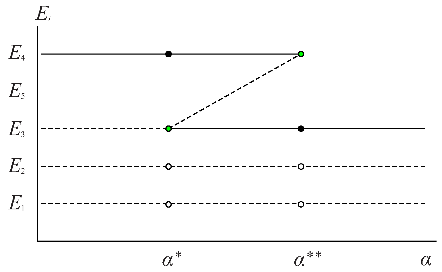
In summary, Proposition 2 establishes conditions in terms of the parameter $\alpha$ that determine the biological sense of the equilibrium points or their collision.

Proposition 2. 

If $q>\eta$, the biological sense of equilibria $E_4$ and $E_5$ in system (1) depends on the parameter α, the maximum per capita consumption rate of the predator, as follows:

1. 

If $\alpha <{\alpha }^{*}$ then ${\overline{B}}_4>0$ and ${\overline{B}}_5<0$, meaning only $E_4=\left({\overline{B}}_4,k\right)$ has biological sense.

2. 

If $\alpha ={\alpha }^{*}$ then ${\overline{B}}_4>0$ and ${\overline{B}}_5=0$, indicating that $E_4=\left({\overline{B}}_4,k\right)$ has biological sense, and $E_5=E_3=\left(0,k\right)$.

3. 

If ${\alpha }^{*}<\alpha <{\alpha }^{**}$ then ${\overline{B}}_4>0$ and ${\overline{B}}_5>0$, meaning $E_4=\left({\overline{B}}_4,k\right)$ and $E_5=\left({\overline{B}}_5,k\right)$ have biological sense.

4. 

If $\alpha ={\alpha }^{**}$ then ${\overline{B}}_4={\overline{B}}_5>0$, indicating that $E_4=E_5=\left({\overline{B}}_4,k\right)$ has biological sense.

5. 

If $\alpha >{\alpha }^{**}$ then ${\overline{B}}_4\notin \mathbb{R}$ and ${\overline{B}}_5\notin \mathbb{R}$, meaning $E_4=\left({\overline{B}}_4,k\right)$ and $E_5=\left({\overline{B}}_5,k\right)$ lack biological sense.

Proof. 

1. If $\alpha <{\alpha }^{*}$, then it follows from (6) that $\alpha <{\alpha }^{**}$; hence, from (5) it can be deduced that ${\overline{B}}_4\in \mathbb{R}$ and ${\overline{B}}_5\in \mathbb{R}$. Additionally, note from (3) and (4) that if $\alpha <{\alpha }^{*}$ then ${\overline{B}}_4>0$ because $q>\eta$ and, furthermore, ${\overline{B}}_5<0$. Therefore, only $E_4=\left({\overline{B}}_4,k\right)$ has biological sense.

2.

Considering that $q>\eta$ and substituting $\alpha ={\alpha }^{*}$ into (3) and (4), we obtain

$$\begin{array}{cc}\hfill {\overline{B}}_4& =\frac{\left(q-\eta \right)+\sqrt{{\left(q-\eta \right)}^2}}{2}=\frac{2\left(q-\eta \right)}{2}=q-\eta >0\hfill \\ \hfill {\overline{B}}_5& =\frac{\left(q-\eta \right)-\sqrt{{\left(q-\eta \right)}^2}}{2}=0.\hfill \end{array}$$

Hence, $E_4=\left({\overline{B}}_4,k\right)$ has biological sense, and $E_5=E_3=\left(0,k\right)$.

3.

First, if $\alpha <{\alpha }^{**}$ it follows from (5) that ${\overline{B}}_4\in \mathbb{R}$ and ${\overline{B}}_5\in \mathbb{R}$. Moreover, from (3), it is clear that ${\overline{B}}_4>0$ because $q>\eta$. Second, if ${\alpha }^{*}<\alpha$ then

$$\begin{array}{cc}\hfill {\alpha }^{*}-\alpha & <0\hfill \\ \hfill 0& >\frac{\eta \omega }{k}-\alpha \hfill \\ \hfill 0& >\frac{4kq}{\omega }\left(\frac{\eta \omega }{k}-\alpha \right)\hfill \\ \hfill {\left(q-\eta \right)}^2& >{\left(q-\eta \right)}^2+\frac{4kq}{\omega }\left(\frac{\eta \omega }{k}-\alpha \right)\hfill \\ \hfill q-\eta & >\sqrt{{\left(q-\eta \right)}^2+\frac{4kq}{\omega }\left(\frac{\eta \omega }{k}-\alpha \right)},\hfill \end{array}$$

where the absolute value was omitted on the left side because $q-\eta >0$. Then,

$$\left(q-\eta \right)-\sqrt{{\left(q-\eta \right)}^2+\frac{4kq}{\omega }\left(\frac{\eta \omega }{k}-\alpha \right)}>0$$

and, therefore,

$${\overline{B}}_5=\frac{\left(q-\eta \right)-\sqrt{{\left(q-\eta \right)}^2+\frac{4kq}{\omega }\left(\frac{\eta \omega }{k}-\alpha \right)}}{2}>0.$$

According to the above, both $E_4=\left({\overline{B}}_4,k\right)$ and $E_5=\left({\overline{B}}_5,k\right)$ have biological sense.

4.

If $\alpha ={\alpha }^{**}$, from expression (5), it follows that

$${\left(q-\eta \right)}^2+\frac{4kq}{\omega }\left(\frac{\eta \omega }{k}-\alpha \right)=0,$$

which means that the radicands in (3) and (4) become zero. Therefore,

$${\overline{B}}_4={\overline{B}}_5=\frac{q-\eta }{2}>0,$$

because, by hypothesis, $q>\eta$. It is then concluded that $E_4=E_5=\left({\overline{B}}_4,k\right)$ has biological sense.

5.

If $\alpha >{\alpha }^{**}$, from expression (5), it follows that

$${\left(q-\eta \right)}^2+\frac{4kq}{\omega }\left(\frac{\eta \omega }{k}-\alpha \right)<0,$$

which implies, according to (3) and (4), that ${\overline{B}}_4\notin \mathbb{R}$ and ${\overline{B}}_5\notin \mathbb{R}$; therefore, $E_4=\left({\overline{B}}_4,k\right)$ and $E_5=\left({\overline{B}}_5,k\right)$ lack biological sense.

   □

Next, we will state and prove Proposition 3, which analyzes the stability of equilibrium points $E_1$, $E_2$, and $E_3$ of system (1).

Proposition 3. 

The stability of equilibrium points $E_1$, $E_2$, and $E_3$ of system (1) is as follows:

1. 

$E_1=\left(0,0\right)$ is unstable (source);

2. 

$E_2=\left(q,0\right)$ is unstable (saddle);

3. 

$E_3=\left(0,k\right)$ is unstable (saddle) if $\alpha <{\alpha }^{*}$, and is locally asymptotically stable if $\alpha >{\alpha }^{*}$ and there is a transcritical bifurcation at this equilibrium point in the bifurcation value $\alpha ={\alpha }^{*}$.

Proof. 

The Jacobian matrix of the system (1) is given by

$$J\left(B,R\right)=\left(\begin{array}{cc}\omega -\frac{2\omega B}{q}-\frac{\alpha \eta R}{{\left(B+\eta \right)}^2}& -\frac{\alpha B}{B+\eta }\\ \frac{\alpha \epsilon \eta R}{{\left(B+\eta \right)}^2}\left(1-\frac{R}{k}\right)& \left(r+\frac{\alpha \epsilon B}{B+\eta }\right)\left(1-\frac{2R}{k}\right)\end{array}\right).$$

(7)

The proof involves evaluating the Jacobian matrix (7) at each equilibrium point $E_i$, $i=1,2,3$, which is denoted as $J\left(E_i\right)$, and calculating the eigenvalues in each case. For hyperbolic equilibrium points, stability conclusions are obtained based on the sign of the real part of the eigenvalues, following the methodology of the Hartman–Grobman theorem [28]. For the nonhyperbolic equilibrium point, the Sotomayor theorem is used to demonstrate the occurrence of a transcritical bifurcation [28]:

1.

The eigenvalues of $J\left(E_1\right)=J\left(0,0\right)$ are ${\lambda }_1=\omega$ and ${\lambda }_2=r$. Since both eigenvalues are positive, we conclude that $E_1$ is an unstable equilibrium point of the source type.

2.

The eigenvalues of $J\left(E_2\right)=J\left(q,0\right)$ are ${\lambda }_1=-\omega$ and ${\lambda }_2=r+\frac{q\alpha \epsilon }{q+\eta }$, allowing us to conclude that $E_2$ is an unstable equilibrium point of the saddle type.

3.

The matrix $J\left(E_3\right)=J\left(0,k\right)$ has the following eigenvalues:

$$\begin{array}{cc}\hfill {\lambda }_1& =\omega -\frac{k\alpha }{\eta }=-\frac{k}{\eta }\left(\alpha -{\alpha }^{*}\right)\hfill \\ \hfill {\lambda }_2& =-r.\hfill \end{array}$$

As ${\lambda }_2<0$, the stability type of equilibrium point $E_3$ depends on the sign of ${\lambda }_1$, which, in turn, depends on whether $\alpha$ is less than, equal to, or greater than ${\alpha }^{*}$. Thus, if $\alpha <{\alpha }^{*}$ then ${\lambda }_1>0$, and, therefore, $E_3$ is an unstable equilibrium point of the saddle type. And if $\alpha >{\alpha }^{*}$, then ${\lambda }_1<0$ and, thus, the equilibrium point $E_3$ is a locally asymptotically stable sink. The case $\alpha ={\alpha }^{*}$ results in ${\lambda }_1=0$. Consequently, equilibrium point $E_3$ is nonhyperbolic, and the occurrence of the bifurcation is demonstrated by verifying that the conditions of Sotomayor’s theorem for the case of transcritical bifurcation are satisfied [28]. In this case, $\mathbf{v}={(1,0)}^T$ and $\mathbf{w}={(1,0)}^T$ are the eigenvectors associated with the zero eigenvalue of the matrices $J\left(E_3\right)$ and $J^T\left(E_3\right)$, respectively. And the vector field associated with system (1) is

$$\mathbf{f}\left(B,R\right)=\left(\begin{array}{c}\omega B\left(1-\frac{B}{q}\right)-\frac{\alpha B}{B+\eta }R\\ \left(r+\epsilon \frac{\alpha B}{B+\eta }\right)R\left(1-\frac{R}{k}\right)\end{array}\right),$$

(8)

from where ${\mathbf{f}}_{\alpha }\left(B,R,\alpha \right)={\left(-\frac{B}{B+\eta }R,\epsilon \frac{B}{B+\eta }R\left(1-\frac{R}{k}\right)\right)}^T$. Then,

$${\mathbf{w}}^T{\mathbf{f}}_{\alpha }\left(0,k,{\alpha }^{*}\right)=\left(1,0\right)\left(\begin{array}{c}0\\ 0\end{array}\right)=0.$$

(9)

On the other hand, since

$$D{\mathbf{f}}_{\alpha }\left(B,R,\alpha \right)=\left(\begin{array}{cc}-\frac{\eta R}{{\left(B+\eta \right)}^2}& -\frac{B}{B+\eta }\\ \frac{\epsilon \eta R}{{\left(B+\eta \right)}^2}\left(1-\frac{R}{k}\right)& \frac{\epsilon B\left(k-2R\right)}{\left(B+\eta \right)k}\end{array}\right),$$

it follows that

$${\mathbf{w}}^T\left[D{\mathbf{f}}_{\alpha }\left(0,k,{\alpha }^{*}\right)\mathbf{v}\right]=\left(1,0\right)\left[\left(\begin{array}{cc}-\frac{k}{\eta }& 0\\ 0& 0\end{array}\right)\left(\begin{array}{c}1\\ 0\end{array}\right)\right]=-\frac{k}{\eta }\ne 0.$$

(10)

Finally, applying $D^2\mathbf{f}\left(B,R,\alpha \right)\left(\mathbf{v},\mathbf{v}\right)=D\left(D\mathbf{f}\left(B,R,\alpha \right)\mathbf{v}\right)\mathbf{v}$ to vector field (8) with $\mathbf{v}={(1,0)}^T$, we obtain

$$D^2\mathbf{f}\left(B,R,\alpha \right)\left(\mathbf{v},\mathbf{v}\right)=\left(\begin{array}{c}\frac{2\alpha \eta R}{{\left(B+\eta \right)}^3}-\frac{2\omega }{q}\\ -\frac{2\alpha \eta \epsilon }{{\left(B+\eta \right)}^3}R\left(1-\frac{R}{k}\right)\end{array}\right).$$

(11)

Then,

$${\mathbf{w}}^T\left[D^2\mathbf{f}\left(0,k,{\alpha }^{*}\right)\left(\mathbf{v},\mathbf{v}\right)\right]=\left(1,0\right)\left(\begin{array}{c}2\omega \left(\frac{1}{\eta }-\frac{1}{q}\right)\\ 0\end{array}\right)=2\omega \left(\frac{1}{\eta }-\frac{1}{q}\right)\ne 0.$$

(12)

Once conditions (9), (10) and (12) are verified, the proposition is proven.

   □

From Proposition 2, it is known that the equilibrium point $E_4=\left({\overline{B}}_4,k\right)$ makes biological sense if $\alpha \le {\alpha }^{**}$ and that the equilibrium point $E_5=\left({\overline{B}}_5,k\right)$ makes biological sense and does not collide with other equilibrium points if ${\alpha }^{*}<\alpha <{\alpha }^{**}$. Therefore, in Proposition 4, the stability of $E_4$ and $E_5$ is analyzed based on these same conditions.

Proposition 4. 

The stability of equilibrium points $E_4$ and $E_5$ of system (1) depends on the value of α, the maximum per capita consumption rate of the predator, as follows:

1. 

If $\alpha <{\alpha }^{**}$ then $E_4=\left({\overline{B}}_4,k\right)$ is locally asymptotically stable.

2. 

If ${\alpha }^{*}<\alpha <{\alpha }^{**}$ then $E_5=\left({\overline{B}}_5,k\right)$ is unstable of the saddle type.

3. 

If $\alpha ={\alpha }^{**}$ then $E_5=E_4=\left({\overline{B}}_4,k\right)$ and, at this equilibrium point, a saddle-node bifurcation occurs.

Proof. 

To simplify the writing of this proof, we denote $\Delta$ as the radicand in (3) and (4), which is given by

$$\Delta ={\left(q-\eta \right)}^2+\frac{4kq}{\omega }\left(\frac{\eta \omega }{k}-\alpha \right).$$

(13)

1.

When evaluating the Jacobian matrix (7) at $E_4$, we obtain $J\left(E_4\right)$, which is given by

$$J\left(E_4\right)=J\left({\overline{B}}_4,k\right)=\left(\begin{array}{cc}\omega -\frac{2\omega {\overline{B}}_4}{q}-\frac{k\alpha \eta }{{\left({\overline{B}}_4+\eta \right)}^2}& -\frac{\alpha {\overline{B}}_4}{{\overline{B}}_4+\eta }\\ 0& -r-\frac{k\alpha \epsilon }{{\overline{B}}_4+\eta }\end{array}\right)$$

and it has the following eigenvalues:

$$\begin{array}{cc}\hfill {\lambda }_1& =\frac{\omega {\left({\overline{B}}_4+\eta \right)}^2\left(q-2{\overline{B}}_4\right)-kq\alpha \eta }{q{\left({\overline{B}}_4+\eta \right)}^2}\hfill \end{array}$$

(14)

$$\begin{array}{cc}\hfill {\lambda }_2& =-r-\frac{k\alpha \epsilon }{{\overline{B}}_4+\eta }.\hfill \end{array}$$

(15)

By substituting (3) and (13) into (14), we obtain

$$\begin{array}{cc}\hfill {\lambda }_1& =\frac{\omega {\left(\frac{q-\eta +\sqrt{\Delta }}{2}+\eta \right)}^2\left(q-2\frac{q-\eta +\sqrt{\Delta }}{2}\right)-kq\alpha \eta }{q{\left(\frac{q-\eta +\sqrt{\Delta }}{2}+\eta \right)}^2}\hfill \\ \hfill & =\frac{\omega {\left(q+\eta +\sqrt{\Delta }\right)}^2\left(\eta -\sqrt{\Delta }\right)-4kq\alpha \eta }{q{\left(q+\eta +\sqrt{\Delta }\right)}^2}\hfill \\ \hfill & =\frac{-\omega \left[{\Delta }^{\frac{3}{2}}+2q\Delta +\left(q+\eta \right)\left(q-\eta \right)\sqrt{\Delta }\right]}{q{\left(q+\eta +\sqrt{\Delta }\right)}^2}.\hfill \end{array}$$

From (5) and (13), we know that if $\alpha <{\alpha }^{**}\iff \Delta >0$ then ${\lambda }_1\ne 0$. And, since $q>\eta$ then $q-\eta >0$, which is a sufficient condition to guarantee that ${\lambda }_1<0$. Now, we substitute (3) and (13) into (15) to obtain

$${\lambda }_2=-r-\frac{k\alpha \epsilon }{\frac{q-\eta +\sqrt{\Delta }}{2}+\eta }=-r-\frac{2k\alpha \epsilon }{q+\eta +\sqrt{\Delta }}<0.$$

We conclude that the equilibrium point $E_4$ is locally asymptotically stable because ${\lambda }_1<0$ and ${\lambda }_2<0$.

2.

When evaluating the Jacobian matrix (7) at $E_5$, we obtain $J\left(E_5\right)=J\left({\overline{B}}_5,k\right)$, the eigenvalues of which are given by

$$\begin{array}{cc}\hfill {\lambda }_1& =\frac{\omega {\left({\overline{B}}_5+\eta \right)}^2\left(q-2{\overline{B}}_5\right)-kq\alpha \eta }{q{\left({\overline{B}}_5+\eta \right)}^2}\hfill \end{array}$$

(16)

$$\begin{array}{cc}\hfill {\lambda }_2& =-r-\frac{k\alpha \epsilon }{{\overline{B}}_5+\eta }.\hfill \end{array}$$

(17)

Substituting (4) and (13) into (16), we obtain

$$\begin{array}{cc}\hfill {\lambda }_1& =\frac{\omega {\left(\frac{q-\eta -\sqrt{\Delta }}{2}+\eta \right)}^2\left(q-2\frac{q-\eta -\sqrt{\Delta }}{2}\right)-kq\alpha \eta }{q{\left(\frac{q-\eta -\sqrt{\Delta }}{2}+\eta \right)}^2}\hfill \\ \hfill & =\frac{\omega {\left(q+\eta -\sqrt{\Delta }\right)}^2\left(\eta +\sqrt{\Delta }\right)-4kq\alpha \eta }{q{\left(q+\eta -\sqrt{\Delta }\right)}^2}\hfill \\ \hfill & =\frac{2q\sqrt{\Delta }\left(q\omega -2k\alpha +\eta \omega -\omega \sqrt{\Delta }\right)}{q{\left(q+\eta -\sqrt{\Delta }\right)}^2}.\hfill \end{array}$$

Again, from (5) and (13), we know that if $\alpha <{\alpha }^{**}\iff \Delta >0$ then the first factor in the numerator is positive. Next, we show that if $\alpha >{\alpha }^{*}$ then the second factor in the numerator is positive. Indeed, if $\alpha >{\alpha }^{*}$ then

$$\begin{array}{cc}\hfill 4k^2\alpha \left(\alpha -\frac{\eta \omega }{k}\right)& >0\hfill \\ \hfill 4k^2{\alpha }^2-4k\alpha \eta \omega & >0.\hfill \end{array}$$

On both sides of this last inequality, we add the expression

$$q^2{\omega }^2+2q\eta {\omega }^2-4kq\alpha \omega +{\eta }^2{\omega }^2$$

and then it is factored to obtain

$$\begin{array}{cc}\hfill {\left(q\omega -2k\alpha +\eta \omega \right)}^2& >q^2{\omega }^2+2q\eta {\omega }^2-4kq\alpha \omega +{\eta }^2{\omega }^2\hfill \\ \hfill {\left(q\omega -2k\alpha +\eta \omega \right)}^2& >{\omega }^2\left[{\left(q-\eta \right)}^2+\frac{4kq}{\omega }\left(\frac{\eta \omega }{k}-\alpha \right)\right]\hfill \\ \hfill {\left(q\omega -2k\alpha +\eta \omega \right)}^2& >{\omega }^2{\Delta }^2\hfill \\ \hfill q\omega -2k\alpha +\eta \omega & >\omega \sqrt{\Delta }\hfill \\ \hfill q\omega -2k\alpha +\eta \omega -\omega \sqrt{\Delta }& >0.\hfill \end{array}$$

It has been shown that ${\lambda }_1>0$. Now, we substitute (4) and (13) into (17) to obtain

$${\lambda }_2=-r-\frac{k\alpha \epsilon }{\frac{q-\eta -\sqrt{\Delta }}{2}+\eta }=-r-\frac{2k\alpha \epsilon }{q+\eta -\sqrt{\Delta }}.$$

Next, we show that if $\alpha >{\alpha }^{*}$ then the denominator is positive. To do this, we start with the following fact:

$$4q\eta -\frac{4kq}{\omega }\left({\alpha }^{*}-\alpha \right)>0,$$

then,    

$$\begin{array}{cc}\hfill 2q\eta & >-2q\eta +\frac{4kq}{\omega }\left(\frac{\eta \omega }{k}-\alpha \right)\hfill \\ \hfill q^2+2q\eta +{\eta }^2& >q^2-2q\eta +{\eta }^2+\frac{4kq}{\omega }\left(\frac{\eta \omega }{k}-\alpha \right)\hfill \\ \hfill {\left(q+\eta \right)}^2& >{\left(q-\eta \right)}^2+\frac{4kq}{\omega }\left(\frac{\eta \omega }{k}-\alpha \right)\hfill \\ \hfill q+\eta & >\sqrt{\Delta }\hfill \\ \hfill q+\eta -\sqrt{\Delta }& >0,\hfill \end{array}$$

allowing us to conclude that ${\lambda }_2<0$. Taking into account that ${\lambda }_1>0$ and ${\lambda }_2<0$, we conclude that equilibrium point $E_5$ is unstable, of the saddle type.

3.

In Proposition 2, it was demonstrated that equilibrium point $E_5$ collides with $E_4$ when $\alpha ={\alpha }^{**}$. This same condition makes ${\lambda }_1=0$: that is, equilibrium point $E_4$ is nonhyperbolic. Therefore, we demonstrate the occurrence of the bifurcation by verifying that the conditions of Sotomayor’s theorem for the saddle-node bifurcation case are satisfied. In this case, $\mathbf{v}={(1,0)}^T$ and $\mathbf{w}={\left(-\left(\frac{4kqr}{\omega \left(q^2-{\eta }^2\right)}+\epsilon \right),1\right)}^T$ are the eigenvectors associated with the zero eigenvalue of the matrices $J\left(E_4\right)$ and $J^T\left(E4\right)$, respectively. Using the vector field associated with system (1), as given in (8), we obtain ${\mathbf{f}}_{\alpha }\left(B,R,\alpha \right)={\left(-\frac{B}{B+\eta }R,\epsilon \frac{B}{B+\eta }R\left(1-\frac{R}{k}\right)\right)}^T$. Then,

$$\begin{array}{cc}\hfill {\mathbf{w}}^T{\mathbf{f}}_{\alpha }\left({\overline{B}}_4,k,{\alpha }^{*}\right)& =\left(-\left(\frac{4kqr}{\omega \left(q^2-{\eta }^2\right)}+\epsilon \right),1\right)\left(\begin{array}{c}-\frac{k\left(q-\eta \right)}{q+\eta }\\ 0\end{array}\right)\hfill \\ \hfill & =k\left(\frac{4kqr}{\omega \left(q^2-{\eta }^2\right)}+\epsilon \right)\frac{q-\eta }{q+\eta }\ne 0,\hfill \end{array}$$

(18)

because $q>>\eta$.

Finally, we apply $D^2\mathbf{f}\left(B,R,\alpha \right)\left(\mathbf{v},\mathbf{v}\right)=D\left(D\mathbf{f}\left(B,R,\alpha \right)\mathbf{v}\right)\mathbf{v}$ to vector field (8) with $\mathbf{v}={(1,0)}^T$ to obtain (11). Then,

$$D^2\mathbf{f}\left({\overline{B}}_4,k,{\alpha }^{*}\right)\left(\mathbf{v},\mathbf{v}\right)=\left(\begin{array}{c}-\frac{2\omega }{q}\frac{q-\eta }{q+\eta }\\ 0\end{array}\right)$$

and, thus,

$$\begin{array}{cc}\hfill {\mathbf{w}}^T\left[D^2\mathbf{f}\left({\overline{B}}_4,k,{\alpha }^{*}\right)\left(\mathbf{v},\mathbf{v}\right)\right]& =\left(-\left(\frac{4kqr}{\omega \left(q^2-{\eta }^2\right)}+\epsilon \right),1\right)\left(\begin{array}{c}-\frac{2\omega }{q}\frac{q-\eta }{q+\eta }\\ 0\end{array}\right)\hfill \\ \hfill & =\frac{2\omega }{q}\left(\frac{4kqr}{\omega \left(q^2-{\eta }^2\right)}+\epsilon \right)\frac{q-\eta }{q+\eta }\ne 0,\hfill \end{array}$$

(19)

because $q>>\eta$. Once conditions (18) and (19) are verified, the proposition is proved.

   □

In Figure 2, the biological sense and stability results obtained in Propositions 2–4 are summarized:

4. Numerical Results

To illustrate the biological sense conditions from Proposition 2 and the stability results discussed in Propositions 3 and 4, numerical simulations of model (1) were performed using the parameter values provided in Table 1. It is important to note that these parameter values are used for illustrative purposes and may not necessarily represent reality accurately [29]. Additionally, while many of these values are sourced from the literature, they should not be considered standard values, as different research may use different figures. This can be exemplified by two studies published in 2021 that used the maximum number of CBBs per tree but reported significantly different values.

In [30], a mathematical model based on nonlinear ordinary differential equations describing the interaction between coffee beans and CBBs was analyzed. The population dynamics of the pest were partially governed by logistic growth, and the carrying capacity, defined as the number of CBBs per tree, was assumed to be 20,000 individuals. On the other hand, in [20], the population dynamics, dispersal, and colonization of CBBs in Colombia were studied and, through fieldwork, the number of CBBs per tree was estimated to be 2674. Despite the significant differences in the figures used in these two studies, this work assumes, for illustrative purposes, that the carrying capacity for the CBB population in model (1), denoted as q, is 2674 CBB per tree, as indicated in Table 1.

Now, let us focus on the carrying capacity of the ant population, which is challenging to precisely measure, since the majority of colony individuals remain in the nest, and those that forage do so in restricted time intervals [31]. However, in [14], it was determined through observations in coffee plantations that the average number of ants per branch is five. On the other hand, in [32], fieldwork established that the number of branches per low-stature coffee tree (e.g., the Caturra variety) is 81. Based on this, it is estimated that the carrying capacity for the ant population, denoted as k, is 400 individuals per tree, obtained by approximating the multiplication of (five ants) × (81 branches), as shown in Table 1.

Table 1. Description, value, and bibliographic reference for each parameter used in the simulations of model (1). Units are expressed using the following notation: d = days, b = CBB, and a = ants.

Parameter	Description	Value	Ref.
$\alpha$	Maximum per capita consumption rate of the predator	Varies b·(a·d)−1
$\epsilon$	Conversion rate of biomass by predation	1 a·b−1	[18]
$\eta$	Half-saturation constant	900 b
k	Carrying capacity of the ants	400 a	[14,32]
q	Carrying capacity of the CBB	2674 b	[20]
r	Intrinsic growth rate of the ants	0.0163 d−1	[33]
$\omega$	Intrinsic growth rate of the CBB	0.0345 d−1	[30]

Table 1. Description, value, and bibliographic reference for each parameter used in the simulations of model (1). Units are expressed using the following notation: d = days, b = CBB, and a = ants.

Parameter	Description	Value	Ref.
$\alpha$	Maximum per capita consumption rate of the predator	Varies b·(a·d)−1
$\epsilon$	Conversion rate of biomass by predation	1 a·b−1	[18]
$\eta$	Half-saturation constant	900 b
k	Carrying capacity of the ants	400 a	[14,32]
q	Carrying capacity of the CBB	2674 b	[20]
r	Intrinsic growth rate of the ants	0.0163 d−1	[33]
$\omega$	Intrinsic growth rate of the CBB	0.0345 d−1	[30]

According to Table 1, the equilibrium points $E_1$, $E_2$, and $E_3$ of model (1) are numerically given by

$$E_1=\left(0,0\right),E_2=\left(2674,0\right),E_3=\left(0,400\right).$$

However, the equilibrium points $E_4$ and $E_5$ do not have a fixed numerical representation because their abscissas, given in (3) and (4), respectively, depend on the bifurcation parameter $\alpha$, whose value varies. Nevertheless,

Table 2. Numerical representation of equilibrium points $E_4$ and $E_5$ of system (1).

Condition for $\mathit{\alpha }$	Value of $\mathit{\alpha }$	${\mathit{E}}_4$	${\mathit{E}}_5$
$\alpha <\alpha *$	0.06	$(2042,400)$	$({\overline{B}}_5,400)$ with ${\overline{B}}_5<0$
$\alpha ={\alpha }^{*}$	0.077625	$(1774,400)$	$E_5=(0,400)=E_3$
${\alpha }^{*}<\alpha <{\alpha }^{**}$	0.095	$(1385,400)$	$(388,400)$
$\alpha ={\alpha }^{**}$	0.1030022723	$(887,400)$	$E_5=(887,400)=E_4$
$\alpha >{\alpha }^{**}$	0.11	$({\overline{B}}_4,400)$, ${\overline{B}}_4\notin \mathbb{R}$	$({\overline{B}}_5,400)$, ${\overline{B}}_5\notin \mathbb{R}$

shows some numerical representations of equilibria $E_4$ and $E_5$ for different values of the parameter $\alpha$, providing a numerical summary of Proposition 2.

The numerical simulations of model (1) consist of phase portraits that arise when varying the maximum per capita consumption rate of the predator $\alpha$, with a particular focus on situations generated when this parameter crosses the bifurcation values ${\alpha }^{*}$ and ${\alpha }^{**}$. Figure 3, Figure 4, Figure 5 and Figure 6, created using pplane8.m, an interactive computational tool in MATLAB software, depict the phase portraits of the system. These portraits exhibit an important generality: in all cases, equilibrium point $E_1$ is an unstable source and equilibrium point $E_2$ is an unstable saddle, as demonstrated in Proposition 3.

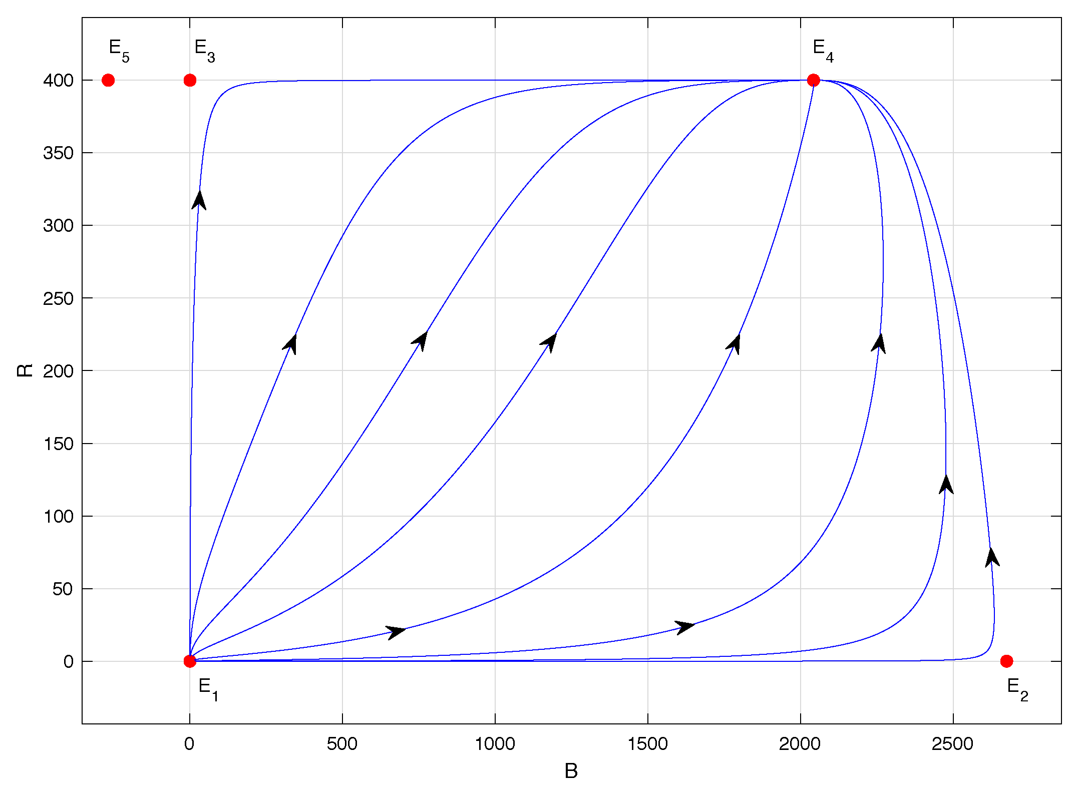
Figure 3 corresponds to the phase portrait of model (1) when $\alpha <{\alpha }^{*}$. In this case, equilibrium point $E_3$ is unstable, of the saddle type, equilibrium point $E_4$ is locally asymptotically stable, and equilibrium point $E_5$ lacks biological sense because its abscissa is negative. In this scenario, the populations co-exist regardless of the initial conditions, and the highest number of CBBs is observed—specifically, approximately 2042 individuals, according to Table 2. This situation is associated with the lowest assumed value for the maximum per capita consumption rate of the predator $\alpha$: namely, $\alpha =0.06$. In fact, as $\alpha \to 0$, $E_4\to \left(q,k\right)$.

For $\alpha ={\alpha }^{*}$, the phase portrait is not shown, as it is similar to that presented in Figure 3. However, it should be noted that in this case, equilibrium point $E_5$ collides with $E_3$, and the abscissa of equilibrium point $E_4$ is reduced. Specifically, for $\alpha =0.077625$, ${\overline{B}}_4$ corresponds to approximately 1774 CBB individuals, according to Table 2.

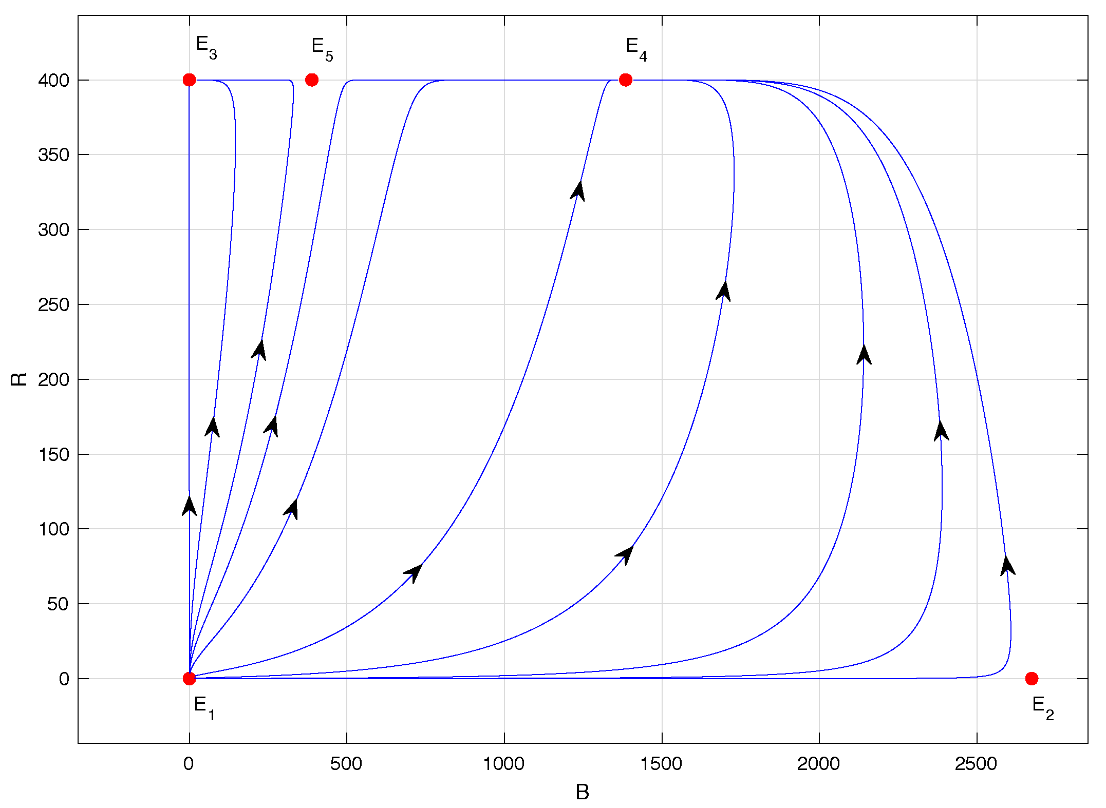
Figure 4 shows the phase portrait of model (1) when ${\alpha }^{*}<\alpha <{\alpha }^{**}$; specifically, $\alpha =0.095$. In this case, equilibrium points $E_3$ and $E_4$ are locally asymptotically stable. However, the latter has a significantly reduced abscissa compared to the previous case; specifically, ${\overline{B}}_4=1385$ according to Table 2. The main novelty in this scenario is the biological sense of equilibrium point $E_5$, which is also unstable, of the saddle type, in accordance with Propositions 2 and 4.

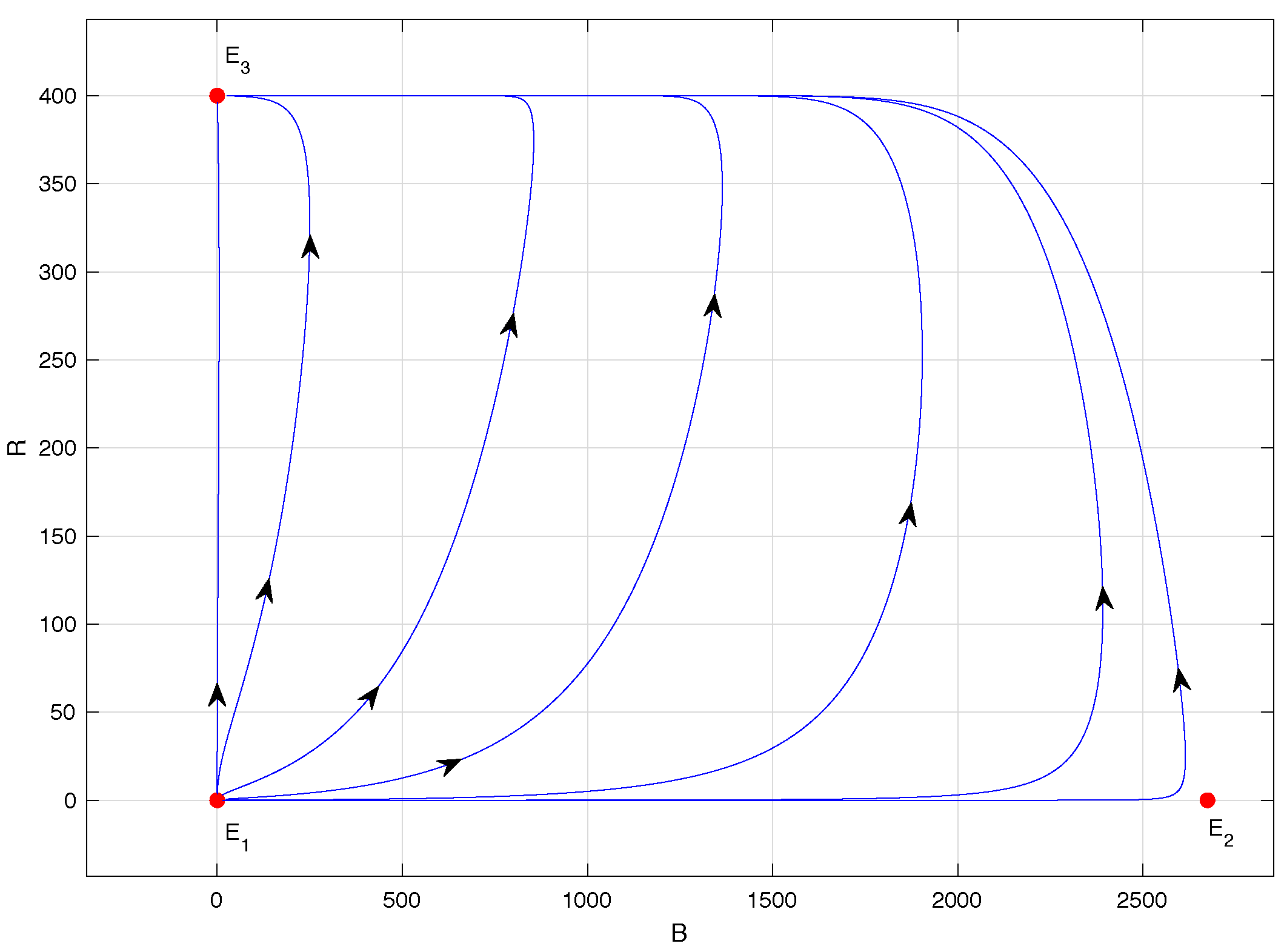
Figure 5 corresponds to the phase portrait of model (1) when $\alpha ={\alpha }^{**}$. In this case, equilibrium point $E_3$ remains locally asymptotically stable, and equilibrium point $E_5$ collides with $E_4$, giving rise to a saddle-node bifurcation, as stated in Proposition 4. Equilibrium point $E_4$ becomes unstable, of the saddle-node type, a denomination given in [28], and now has a much-reduced abscissa: precisely, $E_4=\left(887,400\right)$ for $\alpha ={\alpha }^{**}=0.1030022723$.

Finally, in Figure 6, the phase portrait of model (1) when $\alpha >{\alpha }^{**}$ is shown, specifically for $\alpha =0.11$. This scenario is ideal for the coffee grower because it corresponds to the extinction of the CBB population. Indeed, equilibrium points $E_4$ and $E_5$ lose their biological sense and $E_3$ is locally asymptotically stable. This means that any initial condition within the region $\Omega$ given in (2) will lead to trajectories that asymptotically approach equilibrium point $E_3$, except for initial conditions of the form $\left(B\left(0\right),0\right)$, i.e., those located on the B-axis where the ant population is zero.

It is important to highlight that the trajectories in Figure 3, Figure 4, Figure 5 and Figure 6 provide a visual representation of the system dynamics and that the initial conditions have been carefully chosen to ensure that the associated trajectories illustrate the local and asymptotic stability or instability of the different equilibrium points. Furthermore, the different trajectories highlight the system’s sensitivity to initial conditions and how small variations in these can have a significant impact on its long-term behavior. In the particular case of Figure 4 and Figure 5, where the dynamics of system (1) are illustrated when ${\alpha }^{*}<\alpha \le {\alpha }^{**}$, the initial concentrations of CBBs and ants play a crucial role in the evolution of the CBB population concerning its extinction. This aspect is intrinsically related to the configuration of the stable manifold and the basins of attraction defined by equilibrium points $E_3$ and $E_4$. The stable manifold of $E_5$ in Figure 4 and the stable manifold of $E_4$$(E_4=E_5)$ in Figure 5 define these basins of attraction. Depending on the initial position with respect to these stable manifolds, the system trajectories may converge towards one of the equilibrium points that have been identified as locally and asymptotically stable, determining the persistence or extinction of the CBB population. This analysis underscores the importance of considering initial conditions in the planning of control strategies for CBB in coffee plantations.

5. Discussion

Mathematical models are relatively sophisticated representations of reality, but they are not exact. Their utility lies in their role as substitutes for scientific experiments. In the field of population ecology, mathematical models play a fundamental role as they are crucial for developing theoretical foundations related to the factors that influence population size [34]. This importance is evident in the predator–prey model formulated and studied in this work, as it establishes conditions in terms of the parameter $\alpha$ that determine the co-existence of the two considered populations: CBB and an unspecified species of predatory ants, or the extermination of the pest.

The parameter $\alpha$ corresponds to the maximum per capita consumption rate of the predator, and it is clear from Table 2 that increasing its value disadvantages the CBB population. Indeed, by increasing the value of $\alpha$, the CBB population located at the abscissa of equilibrium point $E_4$ decreases. The above statement can be corroborated by Figure 3, Figure 4, Figure 5 and Figure 6. Note that when the value of the parameter $\alpha$ is low, specifically $\alpha <{\alpha }^{*}$, Figure 3 indicates that the populations co-exist, and the same situation occurs for $\alpha ={\alpha }^{*}$, although this scenario is not shown. However, for ${\alpha }^{*}<\alpha \le {\alpha }^{**}$, Figure 4 and Figure 5 show that increasing $\alpha$ starts to be useful. In these cases, some initial conditions lead to trajectories that asymptotically approach equilibrium point $E_3$, highlighting the possibility of the CBB population going extinct. Fortunately, a sufficient increase in $\alpha$, specifically $\alpha >{\alpha }^{**}$, guarantees the extinction of the CBB population, as observed in Figure 6, where the only locally asymptotically stable equilibrium point is $E_3$. This means that any initial condition in $\Omega$ where the ant population is not zero will lead to trajectories that asymptotically approach equilibrium point $E_3$.

Taking into account the previous discussion, it is concluded that an increase in the bifurcation parameter $\alpha$ significantly reduces the CBB population, suggesting that ant predation is an effective control strategy, at least theoretically. In other words, an effective strategy to mitigate the impact of CBBs in coffee plantations is to stimulate an increase in the ant’s predation rate. This can be achieved by eliminating potential food sources in the crops, as assumed in the proposed model, where ants obtain nutrients from sources other than CBB.

An important aspect to highlight in the results of this work is that regardless of whether the populations co-existed or the CBB population went extinct, the ant population always tended to its carrying capacity, as occurs in reality. In other words, according to the stability results of Propositions 3 and 4, and by Figure 3, Figure 4, Figure 5 and Figure 6, the equilibrium points that were locally and asymptotically stable, i.e., $E_3$ and $E_4$, had an ordinate of k. This means that in any stability situation, the ant population would always tend to its carrying capacity, corresponding to a natural logistic growth behavior. This situation arose because the conversion of CBB biomass into ant biomass was modeled as an extra increase in intrinsic growth attributed to predation. Hence, from the obtained results, it can be suggested that the second differential equation of system (1) is a better choice in modeling than the usual form $\frac{dR}{dt}=rR\left(1-\frac{R}{k}\right)+\epsilon \frac{\alpha B}{B+\eta }R$. In fact, if this latter differential equation is incorporated into model (1), the equilibria $E_4$ and $E_5$ no longer have the ordinate k.

As a future work, it is proposed to incorporate other types of control for CBBs, such as cultural control when the presence of ants with a predatory role is not sufficient to mitigate the effects of CBBs, i.e., when the maximum per capita consumption rate of the predator $\alpha$ satisfies $\alpha \le {\alpha }^{**}$. Cultural control aims to minimize the availability of food and shelter for the pest through the implementation of various manual practices, such as frequent and efficient harvesting of ripe beans in the plantation or the use of homemade traps with alcoholic attractants [9]. Assuming that this capture is carried out based on the quantity of CBB in the crop, we can consider the application of cultural control if the amount of CBB in the coffee field exceeds or does not meet a certain threshold. In this way, the system dynamics can be modeled with a more comprehensive approach that takes into account both the effects of biological control and cultural control, which can be achieved with PieceWise Smooth (PWS) dynamical systems.