Fuzzy Multi-Item Newsvendor Problem: An Application to Inventory Management

Abstract

This paper proposes a novel approach to the fuzzy newsvendor problem for inventory management applications. The main contributions of the paper are the following: a new credibility estimation is proposed, to explore the neighborhood around the most impactful demand scenarios; a simulation procedure was designed for the different demand scenarios, which allows comparison of the proposed approach with classical and fuzzy multi-item newsvendor problems; a modified genetic algorithm (GA) is introduced to ameliorate previous genetic algorithms in both the generation and evaluation of solutions. The new formulation of the fuzzy newsvendor problem, together with the modified GA, were shown to improve the average profit by up to 55% in problems with low-budget scenarios.

1. Introduction

Every day, a newsvendor needs to buy journals based on an uncertain demand. Assuming that each journal has a fixed cost and selling price, if she/he asks for too many journals and the demand is insufficient, there is a reduction in the profit. On the other hand, if the demand is higher than the number of journals ordered, potential sales do not occur, resulting in “lost profits” [1]. This dilemma of buying more or less newspapers, which is known as the newsvendor problem, can be applied to any problem that deals with perishable goods, such as newspapers, magazines, fresh food, or holiday decorations, e.g., Christmas trees. This type of problem has one planning cycle of useful life with uncertain demand and can be modeled as an inventory management problem. Further, the framework of the newsvendor problem can also be applied to capacity investment problems, which can solve relevant societal challenges, such as medical capacity investments. One example is the establishment of epidemic diffusion models to characterize how transmission evolves with (and without) vaccination [2].

Several solutions can be found for solving various inventory management problems [1,3,4]. When multi-items are considered for perishable goods, one deals with a multi-item newsvendor problem (MINP). In this problem, it is important to consider the number of constraints and their type (cost, service level, etc.), the decision-making policies (e.g., optimizing expected profit, service level, etc.). Often, solutions are found using risk-averse techniques. Further, very often MINPs use probability density functions to model the uncertain demand [5,6,7,8].

However, the demanded probabilistic density functions are difficult to derive in real scenarios, especially for innovative and disruptive products, where there are not sufficient data to accurately predict the demand probability distribution. It is possible to mitigate these limitations by including additional information from human expertise using, e.g., fuzzy systems [9]. Fuzzy logic is a suitable tool for incorporating uncertain demands with a proven effectiveness in solving MINPs [9,10,11]. A fuzzy environment can use few data points to describe uncertainty through meaningful membership functions. Furthermore, fuzzy logic offers an ideal environment for describing the vagueness of human thinking through mathematical operations, defining linguistic terms such as “the demand of a product is around 2000” [12].

The first fuzzy solution to the newsvendor problem and inventory management with perishable goods dates back to 1996 [9]. Analytical analyses in a fuzzy environment are useful for specific cases, where it is possible to study a limited number of items in a well-isolated economic environment [13,14,15,16]. Problems arise when the number of items and their relations increase, leading to highly nonlinear problems, making analytical approaches hard to implement [17]. Most of the recent fuzzy [18,19,20] and non-fuzzy [21,22,23,24,25] solutions have focused on solving highly complex single-item problems, lacking generalization to multi-item problems.

Fuzzy MINP problems are usually solved using metaheuristic algorithms [10,11]. Inspired by real-world phenomena, metaheuristics use computational power to find solutions when the classical methods cannot, due to time and complexity. However, metaheuristics do not always guarantee that the solutions found are optimal. However, they can, at least, provide good results for highly complex optimization problems [26]. Shao proposed a genetic algorithm to solve the newsvendor problem with a fuzzy environment [10]. This paper extended the fuzzy objective functions proposed in [9], with the adoption of credibility theory concepts [27,28], namely using the concepts of possibility, necessity, and credibility of a fuzzy event, as well as the excepted value of a fuzzy variable [29] to derive objective functions for different decision-making policies. Further, in 2011, Taleizadeh [11] studied a variety of metaheuristic algorithms to solve a fuzzy single-period newsvendor problem and also proved the suitability of genetic algorithms for this problem.

This paper proposes the following contributions to the fuzzy multi-item newsvendor problem:

• A new credibility estimation is proposed to explore the neighborhood around the most impactful demand scenarios.
• A simulation procedure is designed for different demand scenarios, allowing the comparison of the different fuzzy MINP approaches.
• The genetic algorithm in [11] is modified to solve the fuzzy multi-item newsvendor problem, enhancing the work of [10] in both the generation and evaluation of solutions.

This paper is organized as follows. Section 2 describes classical and fuzzy multi-item newsvendor problems. The proposed hybrid algorithm used to solve fuzzy multi-item newsvendor problems is presented in Section 3. This section first describes a simulation procedure to generate the demand vectors. Then, the proposed credibility estimation is presented. Finally, the optimization architecture using a modified genetic algorithm with three novel mechanisms is described. Benchmark case studies are described in Section 4. Section 5 presents the obtained results, and the conclusions and future work are presented in Section 6.

2. Multi-Item Newsvendor Problem

This section introduces the formulation of the multi-item newsvendor problem. Section 2.1 presents the classical approach with probabilistic demand curves, and Section 2.2 explains the fundamentals of the fuzzy MINP approach.

2.1. Classical Multi-Item Newsvendor Problem

The newsvendor problem deals with situations where the demand for products or items is uncertain. Ordered items that are unsold or unused become obsolete, incurring a cost to dispose of them. However, when the initial amount of at least one of the items is too small, this causes loss of revenue. The classical formulation suggested in [30] uses a modified form of the original model proposed in 1964 [31]. The form in [30] minimizes the expected cost E, with this being minimization equivalent to maximizing an “expected profit” function. The model of the classical multi-item newsvendor problem is as follows:

$$\min E=\sum _{i=1}^N\left[c_i{x}_i+h_i{\int }_0^{x_i}(x_i-d_i)f_i\left(d_i\right)d\left(d_i\right)+v_i{\int }_{x_i}^{\infty }(d_i-x_i)f_i\left(d_i\right)d\left(d_i\right)\right],$$

(1)

subject to

$$\sum _{i=1}^n{c}_i{x}_i\le B,$$

(2)

where the definition of the variables used in this classical multi-item newsvendor problem, which will be used throughout this paper, are the following:

E	expected cost
n	total number of items (products)
$i(=1,2,\dots ,n$)	an item index
$c_i$	cost per unit of item i
$x_i$	amount to be ordered of item i (stochastic variable)
$h_i$	cost incurred per item i for leftover
$d_i$	demand of item i
$f_i\left(d_i\right)$	probability density function of demand for item i
$v_i$	revenue per unit of item i
B	available budget.

This problem is commonly solved using a generic iterative method, by relaxing the problem constraint, applying the Leibniz rule, and using a Lagrangian optimization with a Lagrangian multiplier. This method is described in detail in [30], and is used for comparison purposes for the results, in Section 5. In order to generalize the uncertain demands, a fuzzy formulation of the MINP was introduced in the past [9] and will be described next.

2.2. Fuzzy Multi-Item Newsvendor Problem

This section describes the fuzzy multi-item newsvendor problem, which proved its effectiveness for solving MINP problems [9,10,11]. First, the definitions of possibility, necessity, credibility, and the expected value of a fuzzy demand are presented. Then, the estimation of possibility, necessity, and credibility is explained. Finally, the estimation of the expected profit, the key point of the fuzzy MINP, is described.

2.2.1. Definitions

The possibility, necessity, and credibility of a fuzzy event, presented in [27,28], are used in this paper. Let a fuzzy variable $\xi$ have a membership function $\mu \left(u\right)$. The concepts of possibility, necessity, and credibility of a fuzzy event $(\xi \ge r)$ can be defined as:

$$\mathrm{Pos}\{\xi \ge r\}=sup\mu \left(u\right),u\ge r$$

(3)

$$\mathrm{Nec}\{\xi \ge r\}=1-sup\mu \left(u\right),u<r$$

(4)

$$\mathrm{Cr}\{\xi \ge r\}=\frac{1}{2}\left[\mathrm{Pos}\{\xi \ge r\}+\mathrm{Nec}\{\xi \ge r\}\right]$$

(5)

where for our application $\xi$ is a fuzzy demand with the membership function $\mu \left(u\right)$, u is the generic demand, and r is a profit value. Considering (3)–(5), the expected value of a fuzzy demand $\xi$ is given by [27]:

$$E\left[\xi \right]={\int }_0^{\infty }\mathrm{Cr}\{\xi \ge r\}dr-{\int }_{-\infty }^0\mathrm{Cr}\{\xi \le r\}dr.$$

(6)

2.2.2. Formulation of the Fuzzy Multi-Item Newsvendor Problem

To formulate this problem, additional variables need to be defined:

$r_i$	retail price per unit $(r_i\ge c_i)$ of item i
$s_i$	salvage value per unit $(r_i\le c_i)$ of item i
${\xi }_i$	fuzzy demand of item i
$f(x_i,{\xi }_i)$	profit function for order quantity $x_i$ and fuzzy demand ${\xi }_i$
$F(\mathbf{x},\mathsf{\Xi })$	total profit for all items, in which $\mathbf{x}=(x_1,x_2,\dots ,x_n)$, $\mathsf{\Xi }=({\xi }_1,{\xi }_2,\dots ,{\xi }_n)$.

The profit function for ith item is given by

$$f(x_i,{\xi }_i)=\left\{\begin{array}{cc}(r_i-c_i)x_i,\hfill & x_i\le {\xi }_i\hfill \\ (r_i-s_i){\xi }_i-(c_i-s_i)x_i,\hfill & x_i>{\xi }_i.\hfill \end{array}\right.$$

(7)

Then, the total profit of the newsvendor is as follows:

$$F(\mathbf{x},\mathsf{\Xi })=\sum _{i=1}^{n}f(x_i,{\xi }_i),$$

(8)

subject to (2), as in the classical problem. The objective is to maximize the expected profit of the newsvendor, which can be formulated as follows:

$$\max E\left[F\right(\mathbf{x},\mathsf{\Xi }\left)\right]$$

(9)

subject to

$$B-\sum _{i=1}^n{c}_i{x}_i\ge 0,$$

(10)

$$x_i\ge 0,$$

(11)

3. Proposed Hybrid Algorithm

In order to solve the fuzzy multi-item newsvendor problem, it is necessary to define a simulation procedure that generates the demand vectors. The simulation procedure proposed to simulate the demand is presented in Section 3.1. A critical issue in the simulation procedure is to estimate the credibility, which is presented in Section 3.2. Afterwards, the proposed optimization architecture using a modified genetic algorithm is presented in Section 3.3.

3.1. Demand Simulation Procedure

This section presents a general simulation procedure for addressing fuzzy multi-item newsvendor problems. Let $\mathsf{\Xi }=({\xi }_1,{\xi }_2,\dots ,{\xi }_n)$ be the vector of fuzzy demands, for all n items. Let $\mu$ be the membership function of $\mathsf{\Xi }$, and ${\mu }_i$ be the membership function of ${\xi }_i$, for $i=1,\dots ,n$.

The simulation must generate a sufficiently large positive number for N demand vectors $u_{ik}$, with $i=1,\dots ,n$, and $k=1,\dots ,N$. This procedure simulates real scenarios by using a diverse range of demand vectors $u_{ik}$, with a greater emphasis on probable vectors, while still accounting for less likely ones. By computing the profit for each demand vector $u_{ik}$ with a given solution, the average profit and profit standard deviation across all vectors can be determined.

Let one assume that ${\mathbf{u}}_k=(u_{i1},u_{i2},\dots ,u_{in})$ is a demand vector of n items. The estimated membership grade of the demand vector is given by

$$\mu \left({\mathbf{u}}_k\right)=\mu \left(u_{1k}\right)\cap \mu \left(u_{2k}\right)\cap \dots \cap \mu \left(u_{nk}\right)=min(\mu \left(u_{1k}\right),\mu \left(u_{2k}\right),\dots \mu \left(u_{nk}\right))$$

(12)

where $\mu \left({\mathbf{u}}_k\right)$ is the estimated membership grade, and $\mu \left(u_{ik}\right)$ is the membership grade associated with each order quantity of an item i, with $i=1,2,\dots ,n$.

The possibility and necessity estimations of multi-item solutions from the demand vectors ${\mathbf{u}}_k$ can now be estimated, respectively, in the following way:

$$\widetilde{\mathrm{Pos}}\{R(x,\xi )\ge R_0\}=\underset{1\le k\le N}{max}\left\{\mu \left(u_k\right)\right|R(x,{\mathbf{u}}_k)\ge R_0\}$$

(13)

$$\widetilde{\mathrm{Nec}}\{R(x,\xi )\ge R_0\}=1-\underset{1\le k\le N}{max}\left\{\mu \left(u_k\right)\right|R(x,{\mathbf{u}}_k)\le R_0\}$$

(14)

where $R(x,{\mathbf{u}}_k)$ is the profit function, N is the total number of random demand vectors, and $R_0$ is a profit target. The estimation of the credibility is based on the previous estimations of possibility and necessity, as follows:

$$\widetilde{\mathrm{Cr}}\{R(x,\xi )\ge R_0\}=\frac{1}{2}\left[\widetilde{\mathrm{Pos}}\{R(x,\xi )\ge R_0\}+\widetilde{\mathrm{Nec}}\{R(x,\xi )\ge R_0\}\right].$$

(15)

This estimation is generic for a solution x and for the kth iteration. It is necessary to estimate the credibility for the complete simulation. The estimation proposed in this paper is described next.

3.2. Proposed Credibility Estimation

The proposed credibility estimation is presented in Algorithm 1. The main objective of this approach is to estimate the credibility of a solution x generating a profit higher than a profit target $R_0$. It repeats the estimation K times until it finds it. Estimations for different profit targets $R_0$ are further used to estimate the expected profit of the solution x.

The demand vector is randomly generated and considers quantities that have a membership grade higher than a ${\alpha }_{cut}$, which are defined by 10% quantiles, and as so can have the following values:

$${\alpha }_{cut}\in T\left({\alpha }_{cut}\right)=[1.0^{-5},0.1,0.2,0.3,0.4,0.5,0.6,0.7,0.8,0.9].$$

(16)

Further, the ${\alpha }_{cut}$ is always equal or greater than the minimum value between the highest membership grades found for both possibility and necessity. The ${\alpha }_{cut}$ progressively increases the minimal membership grade of the randomly generated demand vectors. This is useful because the possibility estimation requires finding the demand vector with the highest membership grade that generates a profit higher than the profit target $R_0$, as defined in (13). In addition, the necessity estimation requires finding the demand vector with the highest membership grade that generates a profit lower than the profit target $R_0$, as defined in (14).

Note also that sometimes, due to the random generation, for low credibility solutions, the necessity estimation can be higher than the possibility estimation. These results are impossible, due to the nature of the problem, and therefore are automatically rejected by the algorithm.

The credibility is mandatory to estimate the expected profit of a solution x, with $x=(x_1,x_2,\dots ,x_n$). To focus resources on plausible values, the profit targets are extracted from the interval defined by

$$\left[-\sum _{i=1}^N{c}_i{x}_i,\sum _{i=1}^N(v_i-c_i)x_i\right].$$

(17)

On the one hand, the interval lower limit corresponds to the scenario where no sales are made. On the other hand, the upper limit corresponds to the scenario where all purchased items are sold.

Assuming that the total number of profit targets is given by S, the profit targets are equally distributed and the set of profit targets are defined by $r=(r_1,r_2,\dots ,r_S)$, where $r_1<r_2<\dots <r_S$. Equations (18)–(20) describe the necessary steps for estimating the expected profit E of a solution x:

$$E_1=-\sum \widetilde{\mathrm{Cr}}\{R(x,{\mathbf{u}}_k)\le r_j\},if{r}_j<0$$

(18)

$$E_2=E_1+\sum \widetilde{\mathrm{Cr}}\{R(x,{\mathbf{u}}_k)\ge r_j\},if{r}_j\ge 0$$

(19)

$$E=E_2\times \frac{(r_S-r_1)}{S}+max(0,r_1)+min(0,r_S)$$

(20)

The number of credibility samples S is a crucial variable in this estimation. This variable must be studied to obtain the best possible trade-off between computational time and accuracy.

Algorithm 1 Credibility Estimation

Require: x; $R_0$; $R(x,{\mathbf{u}}_k)$; $T\left({\alpha }_{cut}\right)$; K ${\alpha }_{cut}\leftarrow T\left({\alpha }_{cut}\right)$ $\widetilde{\mathrm{Pos}}\leftarrow 0$; $\widetilde{\mathrm{Nec}}\leftarrow 0$; $l\leftarrow 0$; $stop\leftarrow False$ while  $stop=False$  do     Compute random ${\mathbf{u}}_k$ with $min(\mu \left(u_{1k}\right),\dots ,\mu \left(u_{nk}\right))\ge {\alpha }_{cut}$     Compute $\mu \left({\mathbf{u}}_k\right)$ using (12)       ====== Possibility and Necessity Update ======     if $R(x,{\mathbf{u}}_k)>R_0$ and $\mu \left({\mathbf{u}}_k\right)>\widetilde{\mathrm{Pos}}$ then         $\widetilde{\mathrm{Pos}}\leftarrow \mu \left({\mathbf{u}}_k\right)$     else if $R(x,{\mathbf{u}}_k)<R_0$ and $\mu \left({\mathbf{u}}_k\right)>\widetilde{\mathrm{Nec}}$ then         $\widetilde{\mathrm{Nec}}\leftarrow \mu \left({\mathbf{u}}_k\right)$       ===========Threshold Update ==========     if $min(\widetilde{\mathrm{Pos}},\widetilde{\mathrm{Nec}})>{\alpha }_{cut}$ then         ${\alpha }_{cut}\leftarrow min(\widetilde{\mathrm{Pos}},\widetilde{\mathrm{Nec}})$ (soft threshold update)     else if $l\ge K$ and ${\alpha }_{cut}\ge max\left(T\left({\alpha }_{cut}\right)\right)$ then         $stop\leftarrow True$ (finish execution)     else if $l\ge K$ then         ${\alpha }_{cut}\leftarrow min(T\left({\alpha }_{cut}\right)>{\alpha }_{cut}$) (hard threshold update)         $l\leftarrow 0$     else         $l\leftarrow l+1$   =========== Finish Execution ========== $\widetilde{\mathrm{Nec}}\leftarrow 1-\widetilde{\mathrm{Nec}}$ if  $\widetilde{\mathrm{Pos}}>\widetilde{\mathrm{Nec}}$  then     Compute $\widetilde{\mathrm{Cr}}\{R(x,\xi )\ge R_0\}$ using (15) else     $\widetilde{\mathrm{Cr}}\{R(x,\xi )\ge R_0\}=0$ (solution rejected)

3.3. Proposed Optimization Architecture

The formulation of the fuzzy newsvendor problem allows its application to inventory problems. This is accomplished with an optimization architecture that combines a modified genetic algorithm (GA) and the expected profit estimation. Along with the common mechanisms of a genetic algorithm, crossover, mutation, and selection [32], novel problem-specific genetic mechanisms are introduced.

The proposed optimization architecture finds the solution $\mathbf{x}=(x_1,x_2,\dots ,x_n)$ with the highest expected profit, according to the fundamentals previously introduced in Section 2. Algorithm 2 details the proposed genetic algorithm for maximizing the expected profit. This algorithm needs to estimate the credibility $\widetilde{\mathrm{Cr}}$, as proposed in Section 3.2 and Algorithm 1. The genetic algorithm used is the one in [10], using classic selection, crossover, and mutation operators. Further, the genetic algorithm also uses the novel problem-specific genetic mechanisms described in the next section.

Algorithm 2 Proposed Genetic Algorithm

Require: G; $i\leftarrow 0$ 1: while  $i<G$  do 2:     for each individual $\mathbf{x}$ of generation i do 3:         Compute profit interval using (17) 4:         Compute all profit targets $r_j$ by equally sample profit interval 5:         Compute the credibility $\widetilde{Cr}\{R(x,\xi )\ge r_j\}$ for all j using Algorithm 1 6:         Compute expected profit $E\left[R\right(x,\xi \left)\right]$ using (18)–(20) 7:     Compute next population using novel GA mechanisms in Section 3.4 8:     $i\leftarrow i+1$ 9: Select the individual x with the highest expected profit E.

3.4. Novel Problem-Specific Genetic Mechanisms

This section describes problem-specific mechanisms, which are implemented in the architecture proposed in Algorithm 2. These methods enhance the set of solutions by (1) discarding items in the initial population, (2) scaling chromosomes according to the available budget, and (3) introducing a problem-specific context to the crossover operator. This section thus proposes chromosome initialization, solution resizing, and chromosome normalization, which are described next.

3.4.1. Initialization with Zero Quantities

The initialization with zero quantities initializes chromosomes with a single non-zero ordering quantity $x_i$. After selecting a random item i for the non-zero ordering quantity, the chromosome is resized as explained in Section 3.4.2 to scale $x_i$ to reach the available budget. If i is a profitable item, the chromosome is selected, because the expected profit is higher than chromosomes containing less profitable items. This mechanism aims to select (and further combine) only the most profitable items.

3.4.2. Solution Resizing

The solution resizing mechanism scales the chromosome ordering quantities $x_i$ to use all the available budget. It scales the quantities up or down without changing the relative proportions between them. On the one hand, this mechanism can transform over-budget solutions into feasible solutions by scaling them down. On the other hand, it can scale up under-budget solutions to use all the available budget. To apply this mechanism, the ordering quantities $x_i$ are resized to quantities $x_{ri}$ by multiplying them by a resizing ratio, as follows:

$$x_{ri}=x_i\times \frac{B}{{\sum }_{i=1}^N{c}_i{x}_i}$$

(21)

3.4.3. Chromosome Normalization

This normalization makes the crossover independent of the absolute values in x, by normalizing them according to the items with the highest expected demand value. In this paper, the highest expected demand value comes from the item with the probabilistic density function $f_i\left(d_i\right)$, but it could also be the fuzzy value with the highest grade. To apply the chromosome normalization, first, the ordering quantities $x_i$ must be normalized by applying the transformation:

$$x_{ni}=\frac{x_i}{u_i}$$

(22)

where $x_i$ is the ordering quantity of item i, $u_i$ is the expected demand value of the probabilistic distribution of item i, and $x_{ni}$ is the normalized ordering quantity of item i. After the crossover has been applied, all normalized ordering quantities $x_{ni}$ must be de-normalized by multiplying them by $u_i$.

4. Case Studies

The two benchmark case studies used in this paper were presented in [10,30,33]. The first numerical example is well known because it is simple (only six products) and it also shows that relaxing the non-negativity constraints sometimes leads to infeasible order quantities. The second example illustrates the application of the proposed approach for a large number of products, 17 in this case. This number is already similar to several real-world scenarios.

The optimization method presented in [30,33] is a generic iterative method (GIM) with two different use cases: one with exponential demand distributions, which is described in Section 4.1, and the other with normal demand distributions, described in Section 4.2.

4.1. Case Study 1: Exponential Demand Distribution

The first case study was proposed in [30] and used in [10], where the item demand is exponentially distributed. An exponential distribution for demand $d_i$ with a mean value $m_i$ is described in (23) and (24), defining its probability density function and cumulative distribution function, respectively.

$$f_i(d_i,m_i)=\left\{\begin{array}{cc}0,\hfill & d_i<m_i\hfill \\ \frac{1}{m_i}{e}^{-\frac{d_i}{m_i}},\hfill & d_i\ge m_i\hfill \end{array}\right.$$

(23)

$$F_i(d_i,m_i)=\left\{\begin{array}{cc}0,\hfill & d_i<m_i\hfill \\ 1-e^{-\frac{d_i}{m_i}},\hfill & d_i\ge m_i.\hfill \end{array}\right.$$

(24)

In [10,30], the exponential demand distribution considered a problem with six items, as presented in

Table 1. Data for Case Study 1: Revenue loss per unit, cost for leftover, cost per unit, and mean of demand for the six items.

Item	${\mathit{v}}_{\mathit{i}}$ (CU)	${\mathit{h}}_{\mathit{i}}$ (CU)	${\mathit{c}}_{\mathit{i}}$ (CU)	${\mathit{m}}_{\mathit{i}}$
1	7	1	4	200
2	12	2	8	225
3	30	4	20	112.5
4	30	4	10	100
5	40	2	13	75
6	45	5	15	30

, and a budget of 3500 currency units (CU).

The GIM proposed in [30] solved this optimization problem by relaxing the problem constraint, applying the Leibniz rule and using a Lagrangian optimization with a Lagrangian multiplier. The obtained solution with the ordering quantities per item is presented in

Table 2. Case Study 1: benchmark solution with ordering quantities per item.

Item	1	2	3	4	5	6
$x_i$	78.41	58.16	30.06	81.74	70.91	25.29

.

4.2. Case Study 2: Normal Demand Distribution

The second case study was proposed in [33], and considers a normal distribution for demand $d_i$. A demand distribution $d_i$ has the mean value $m_i$ and the standard deviation ${\sigma }_i$, see (25) and (26), defining its probability density function and cumulative distribution function, respectively.

$$f_i(d_i,m_i)=\frac{1}{{\sigma }_i\sqrt{2\pi }}{e}^{-\frac{1}{2}{\left(\frac{d_i-m_i}{{\sigma }_i}\right)}^2}$$

(25)

$$F_i(d_i,m_i)=\frac{1}{2}\left[1+erf\left(\frac{d_i-m_i}{\sqrt{2}{\sigma }_i}\right)\right]$$

(26)

where

$$erf\left(x\right)=\frac{1}{\sqrt{\pi }}{\int }_{-x}^x{e}^{-t^2}dt.$$

(27)

This case study includes 17 items, as shown in

Table 3. Data for Case Study 2: Revenue loss per unit, cost for leftover, cost per unit, mean and standard deviation of demand for the 17 items.

Item	${\mathit{v}}_{\mathit{i}}$ (CU)	${\mathit{h}}_{\mathit{i}}$ (CU)	${\mathit{c}}_{\mathit{i}}$ (CU)	${\mathit{m}}_{\mathit{i}}$	${\mathit{\sigma }}_{\mathit{i}}$
1	7	1	4	102	51
2	12	2	8	73	18.3
3	30	4	19	123	30.8
4	30	4	17	95	23.8
5	40	2	23	62	15.5
6	45	5	15	129	43
7	16	1	10	69	34.5
8	21	2	10	83	41.5
9	42	3	40	120	30
10	34	5	20	89	22.3
11	20	3	10	115	38.3
12	15	5	7	91	30.3
13	10	3	4	52	17.3
14	20	3	12	76	38
15	47	2	33	66	16.5
16	35	4	21	147	36.8
17	22	1	11	104	34.7

, and an available budget of 2500 CU.

The expected profit-maximizing solution proposed in [33] is presented in

Table 4. Case Study 2: Benchmark solution with ordering quantities per item.

Item	${\mathit{x}}_{\mathit{i}}$	Item	${\mathit{x}}_{\mathit{i}}$
1	0	10	0
2	0	11	15.58
3	0	12	42.2
4	0	13	34.56
5	0	14	0
6	106.86	15	0
7	0	16	0
8	14.02	17	15.23
9	0

.

4.3. Membership Functions for the Demand

The fuzzy MINP requires the definition of membership functions for the fuzzy demand. This paper considers trapezoidal and exponential membership functions, in order to compare two different types of membership functions.

A trapezoidal membership function is defined by four parameters $(a,b,c,d)$ [34]. These four parameters define five different line segments alongside the complete universe of discourse. A definition of a trapezoidal membership function is given by:

$$\mu (x;a,b,c,d)=max\left(min\left(\frac{x-a}{b-a},1,\frac{d-x}{d-c}\right),0\right).$$

(28)

An exponential membership function is defined, using as parameters the mean value m and the decay ratio d:

$$\mu (x;m,d)=\left\{\begin{array}{cc}{e}^{d\frac{x-m}{m}},\hfill & x\le m\hfill \\ e^{-d\frac{x-m}{m}},\hfill & x>m.\hfill \end{array}\right.$$

(29)

The membership function parameters for Case Study 1 were based on the ones presented in [10]. This paper adjusted them slightly in order to optimize the results, namely we used triangular membership functions that were revealed to be more suitable for the problem. The originals and the ones used in this paper are presented in

Table 5. Membership functions for Case Study 1.

	From [10]		Proposed
Item	Type	Values	Type	Values
1	Trapez.	(180, 190, 210, 220)	Triang.	(180, 200, 200, 220)
2	Trapez.	(210, 220, 230, 240)	Triang.	(210, 225, 225, 240)
3	Trapez.	(100, 110, 115, 125)	Triang.	(100, 112.5, 112.5, 125)
4	Trapez.	(80, 90, 110, 120)	Triang.	(80, 100, 100, 120)
5	Trapez.	(60, 70, 80, 90)	Triang.	(60, 75, 75, 90)
6	Trapez.	(20, 25, 35, 40)	Triang.	(20, 30, 30, 40)

.

For Case Study 2, trapezoidal and exponential membership functions were tested. The exponential ones gave slightly better results and were chosen for use. The membership functions for Case Study 2 are presented in

Table 6. Membership functions selected for Case Study 2.

Proposed
Item	Type	Values	Item	Type	Values
1	Exponential	(102, 6)	10	Exponential	(89, 6)
2	Exponential	(73, 6)	11	Exponential	(115, 6)
3	Exponential	(123, 6)	12	Exponential	(91, 6)
4	Exponential	(95, 6)	13	Exponential	(52, 6)
5	Exponential	(62, 6)	14	Exponential	(76, 6)
6	Exponential	(129, 6)	15	Exponential	(66, 6)
7	Exponential	(69, 6)	16	Exponential	(147, 6)
8	Exponential	(83, 6)	17	Exponential	(104, 6)
9	Exponential	(120, 6)

.

5. Results

This section presents the results using the hybrid algorithm proposed in Section 3. The results are compared with previous classical and fuzzy newsvendor problems. The case studies presented in Section 4 were used to asses the performance of the hybrid algorithm proposed in this paper. These comparisons intend to understand if a more flexible framework—with the ability to incorporate complex profit functions and human expertise—can obtain better results than previous classical and fuzzy approaches that lacked this kind of flexibility.

5.1. Impact of the Genetic Algorithm Parameters

First, the parameters of the genetic algorithm are properly tuned. The first parameters to be explored were the number of generations, which are presented in

Table 7. Tuning of population size. The line in bold is the one with the best fitness.

Case Study	Generat.	Popul. Size	Fitness	Time [s]
1	20	10	4535 ± 210	105
1	20	25	4882 ± 111	156
1	20	50	4918 ± 99	312
1	20	75	5064 ± 23	372
1	20	100	4928 ± 129	510
2	20	10	1948 ± 285	198
2	20	25	2915 ± 49	234
2	20	50	3015 ± 66	472
2	20	75	2959 ± 66	590
2	20	100	3031 ± 49	848

. We tested population sizes between 10 and 100 individuals. We used 20 generations to assure some convergence of the algorithm. The population size that obtained the best fitness for Case Study 1 was 75, and for Case Study 2 it was 50. These parameters were thus fixed to these values.

Table 8. Tuning of the number of generations. The line in bold is the one with the best fitness.

Case Study	Generat.	Popul. Size	Fitness	Time [s]
1	5	75	4935 ± 104	28
1	10	75	5027 ± 53	53
1	15	75	4930 ± 128	128
1	20	75	5064 ± 23	230
1	30	75	4888 ± 103	367
2	5	50	3011 ± 92	153
2	10	50	2994 ± 39	259
2	15	50	3045 ± 57	471
2	20	50	3022 ± 66	593
2	30	50	3014 ± 47	710

presents the test performed in both case studies to find the best number of generations for the genetic algorithm. The problem did not require a large number of generations to converge. Values between 5 and 30 were tested. It was found out that for Case Study 1, 20 iterations gave the best fitness, while 15 generations were the best for Case Study 2.

The tuning of the crossover probability is presented in

Table 9. Tuning of the crossover probability. The line in bold is the one with the best fitness.

Case Study	Crossover Probab.	Fitness
1	0.1	48923 ± 160
1	0.3	4883 ± 69
1	0.5	4950 ± 126
1	0.7	4988 ± 103
1	0.8	5107 ± 57
1	0.9	5067 ± 61
2	0.1	3465 ± 158
2	0.3	3645 ± 89
2	0.5	3650 ± 21
2	0.7	3657 ± 16
2	0.8	3742 ± 44
2	0.9	3725 ± 41

. We tested values from 10% to 90%. For both case studies, the value of 80% was found to give the best results. This is interesting, as this is a very common value chosen for this parameter in genetic algorithms.

Last but not the least, we tested the best value for the probability of mutation in the chromosomes, see

Table 10. Tuning of the mutation probability. The lines in bold are the ones with the best fitnesses.

Case Study	Mutation Probab.	Fitness
1	0.05	4987 ± 98
1	0.1	4924 ± 105
1	0.2	5107 ± 57
1	0.3	4893 ± 64
1	0.4	5002 ± 101
1	0.5	5100 ± 22
1	0.7	4967 ± 135
1	0.9	5016 ± 69
2	0.05	3693 ± 28
2	0.1	3698 ± 34
2	0.2	3742 ± 44
2	0.3	3716 ± 41
2	0.5	3728 ± 28
2	0.7	3701 ± 68
2	0.9	3701 ± 45

. We tested values from 5% to 90%. Please note that very high values (above 70%) can be considered as a random search. The value of 20% was found to be the best value of mutation for both case studies.

Once the usual parameters of the GA had been selected, it was possible to test the impact of the novel problem-specific mechanisms proposed in this paper. This analysis is given next.

5.2. Impact of the Novel Problem-Specific Mechanisms

This section evaluates the impact of the specific features proposed in this paper on the performance of the optimization. Each of the introduced problem-specific generic mechanisms presented in Section 3.4, namely: initialization with zero quantities, solution resizing and chromosome normalization are analyzed separately.

First,

Table 11. Results using initialization with zero quantities. Lines in bold are the ones with the best fitness.

Case Study	Init. with Zero Quantities	Fitness	Simulated Profit
1	Yes	4167.9	2860.3
1	No	4940.9	2853.0
2	Yes	3741.9	3797.3
2	No	2229.9	2446.6

presents the influence of the initialization with zero quantities, introduced in Section 3.4.1. This mechanism proved to be advantageous for Case Study 2. However, it proved to be highly disadvantageous in Case Study 1. Therefore, the effect of this initialization varied significantly between the case studies. This mechanism must then be tested, and used only if it leads to better results.

The effect of the solution resizing introduced in Section 3.4.2 is shown in

Table 12. Results using solution resizing. Lines in bold are the ones with the best fitness.

Case Study	Sol. Resizing	Fitness	Unfeasible Sol.	Simulated Profit
1	Yes	4167.9	0	2860.3
1	No	3945.1	250.4	2293.2
2	Yes	3741.9	0	3797.3
2	No	2208.8	122.2	2305.6

. The solution resizing was primarily implemented to eliminate unfeasible solutions. This effect is emphasized in the table; the number of unfeasible solutions is zero, as expected. But beyond this, it had the effect of increasing the fitness and the profit. Therefore, this feature was always used in the genetic algorithm.

The last modification proposed for introduction in the GA, normalization of the chromosome (which was described in Section 3.4.3), had the results presented in

Table 13. Results using chromosome normalization. Lines in bold are the ones with the best fitness.

Case Study	Chromosome Norm.	Fitness	Simulated Profit
1	Yes	4889.5	2827.4
1	No	4940.9	2853.0
2	Yes	3713.7	3755.7
2	No	3741.9	3797.3

. It can be observed that the performance in terms of fitness and simulated profit was slightly reduced. However, it is recommended to always try this mechanism in different case studies, because it leads to a smaller computational effort (about a 5 to 10% reduction).

5.3. Computational Performance

Scalability is crucial when designing industrial solutions. It is common for real-world inventory management problems to increase the number of items, and thus the number of decision variables. A problem can become impossible to solve in real time when the computational power does not keep up with this increase in dimensions. Thus, computational efficiency is a critical aspect when implementing iterative optimization algorithms, such as genetic algorithms [35,36].

Genetic algorithms are excellent candidates for applying parallel computing. They have several steps where they perform multiple independent tasks, such as fitness evaluation or creation of a population. We used parallelism in the fitness evaluation procedure, since this is the phase with the highest computational cost. The parallel computation was implemented in a cloud environment.

Every program running in the cloud has an environment previously defined by the user. This environment is called a container. The container has all the necessary packages, as well as the source code to be executed. Additionally, the container receives all required variables (in the MINP, the crossover probability, population size, etc.) as environment variables. This results in an isolated and constant environment that allows running a given program for different input variables. With the container defined, it is possible to pass its image to a machine of choice. The device will then execute the tasks described in the source code. Moreover, given a well-defined environment, there will not be any operating incompatibilities during execution. Figure 1 illustrates the overall containerization life cycle.

The ability to perform the same tasks in different machines without altering the source code or conditions is an advantage of containerization.

Table 14. Properties of the virtual machines.

	vCPU	Memory [GB]
Machine 1	2	8
Machine 2	4	16
Machine 3	8	32
Machine 4	16	64
Machine 5	48	192
Machine 6	96	384

presents the characteristics of the set of cloud virtual machines used in this paper. We wanted to find the set exhibiting the best ratio between computational power and performance.

The proposed algorithm was run for both case studies using exponentially distributed demands, considering the different machines in Table 14 and applying parallel computing. Figure 2 shows the relation between the number of virtual CPUs and the run time. For Case Study 2, the more demanding case, Machine 1 had a running time of 9216 s, while Machine 5, the one with the best ratio between power and performance, needed only 340 s to complete the job. The running time reduction between these machines was 96%.

Table 15. Machine 5: Performance with and without parallelism.

	Parallel Execution	Running Time [s]
Machine 5	Yes	340
Machine 5	No	20,342

shows the running time with and without parallelism, both using Machine 5. Without parallel computing, the use of powerful machines becomes irrelevant. Using the integration of parallel computing and cloud resources reduced the computation time by 98.3% (from 5.6 h to less than 6 min). This drastic reduction made problems feasible that were almost impossible to solve due to time constraints. The results obtained in the next section used Machine 5 in a cloud environment with parallelism. The maximum running time was about 8 minutes.

5.4. Main Results

In this section, we present the main results of our study. It compares the performance of three different methods for solving the case studies in Section 4. The first method is the classical approach, introduced in Section 2.1, the second methods is the fuzzy genetic algorithm proposed in [10], and the third is the hybrid algorithm proposed in this paper in Section 3.

Table 16. Simulation results in terms of average profit and standard deviation of the profit.

Case Study	Method	Profit
1	Classical approach	2877.1 ± 2.0
1	Fuzzy GA from [10]	2889.8 ± 1.2
1	Proposed hybrid algorithm	2914.7 ± 1.5
2	Classical approach	3869.4 ± 0.5
2	Fuzzy GA from [10]	2833.6 ± 0.2
2	Proposed hybrid algorithm	3878.7 ± 0.8

presents the obtained results. The GA was run 50 times, and the results show the average and the standard deviation of the obtained profit. It is clear for both case studies that the proposed hybrid algorithm outperformed the other two approaches in terms of profit. In Case Study 1, the simplest case, it was only slightly better than the other approaches. However, in Case Study 2, it significantly outperformed the previous fuzzy approach in [10]. Moreover, it also slightly outperformed the classical approach.

The standard deviation of all approaches was relatively small, showing the effectiveness of the genetic algorithm. For Case Study 1, the proposed algorithm had a smaller standard deviation than the classical approach, but slightly larger than the fuzzy MINP optimized with GA in [10]. In Case Study 2, the proposed algorithm presented a slightly larger standard deviation than the other two approaches, but without affecting the excellent result obtained for the profit.

Summarizing, the proposed hybrid algorithm was able to significantly improve on the previous fuzzy approach and it also slightly improved on the classical approach. The main drawback was its computational demand.

6. Conclusions

A novel approach to the fuzzy newsvendor problem for inventory management applications was proposed in this paper. A hybrid algorithm was proposed to solve fuzzy multi-item newsvendor problems by introducing a simulation procedure to generate the demand vectors. One of the main contributions of this work was the redesigning of a mandatory variable in the simulation procedure, the credibility estimation, which introduced a dynamic adjustment of an ${\alpha }_{cut}$ threshold to generate meaningful demand vectors, instead of using a purely random vector generation. Further, a modified genetic algorithm that discards some products in the initial population, scales the chromosomes according to the available budget, and makes the crossover operator independent of the absolute values of the solutions.

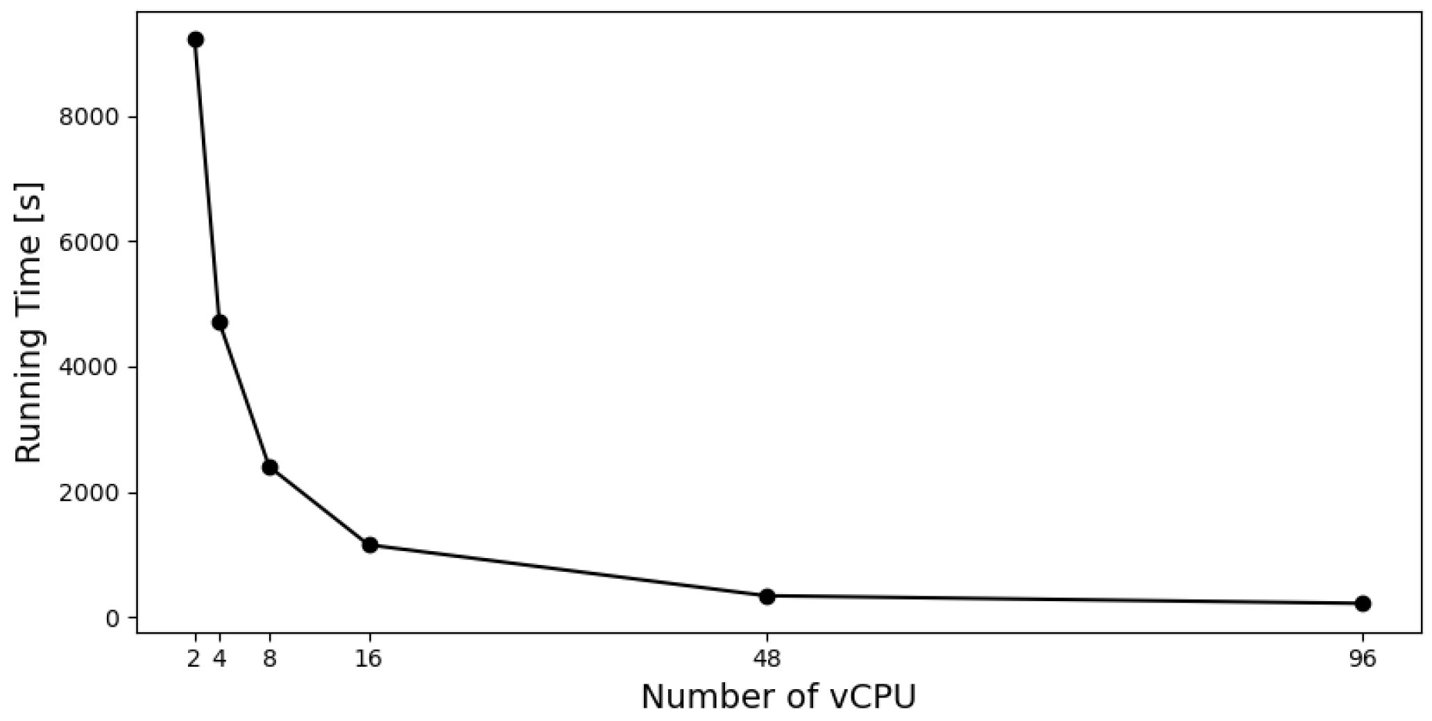
The proposed hybrid algorithm was compared to other classical and fuzzy approaches in two benchmark case studies, and it slightly outperformed the classical approach. However, it clearly outperformed the previous fuzzy approach. In the most complex case, Case Study 2, it improved the profit by 55%. This performance increase was the result of introducing a new initialization with null values, which proved to be a valuable mechanism in low-budget scenarios, where there is the need for rejecting less profitable items. Please note that Case Study 2 already has a high dimension and it is similar to a large number of real-world problems in inventory management. The main limitation of the proposed approach was the computational effort of the algorithm. Using a cloud environment and parallel computing led to low computational times (about 8 min), which is very acceptable. However, these resources can be expensive.

The proposed hybrid algorithm is very flexible. Despite using fixed costs to prove its effectiveness against analytical approaches, this solution can work with nonlinear pricing models. To perform this, one only needs to integrate the pricing information when calculating profits in the credibility estimation. This is suggested for future work. Moreover, there is the possibility of changing performance measures. Profit was used to prove the effectiveness against analytical approaches, but the algorithm could prioritize the solutions that most satisfied possible customer demand, by replacing the profit calculation with a service-level calculation, for instance. We used perhaps the most usual version of a fuzzy number. However, other fuzzy numbers such as Z–numbers [37], G–numbers [38], or R–numbers [39] could be used. This is another avenue of future research. Last but not the least, in the near future, we are going to implement the fuzzy MINP in a model of medical capacity investment, to evaluate the impact of health public policies in terms of infant mortality rates.

References

1. Choi, T.M. Handbook of Newsvendor Problems. International Series in Operations Research & Management Science; Springer: Berlin/Heidelberg, Germany, 2012. [Google Scholar] [CrossRef]
2. Chen, X.; Dong, Y.; Wu, M. Medical capacity investment for epidemic disease: The effects of policymaker’s confidence and public trust. Risk Anal. 2023, 43, 1187–1211. [Google Scholar] [CrossRef] [PubMed]
3. Wilson, E.B. The Mathematical Theory of Investment. Science 1888, 42, 248–249. [Google Scholar] [CrossRef]
4. Mu, M.; Chen, J.; Yang, Y.; Guo, J. The Multi–product Newsvendor Problem: Review and Extensions. In Proceedings of the 2019 6th International Conference on Behavioral, Economic and Socio-Cultural Computing, Beijing, China, 28–30 October 2019; pp. 6–9. [Google Scholar]
5. Lau, H.S.; Lau, A.H.L. The multi-product multi-constraint newsboy problem: Applications, formulation and solution. J. Oper. Manag. 1995, 13, 153–162. [Google Scholar] [CrossRef]
6. Lau, H.S.; Lau, A.H.L. The newsstand problem: A capacitated multiple-product single-period inventory problem. Eur. J. Oper. Res. 1996, 94, 29–42. [Google Scholar] [CrossRef]
7. Shi, J.; Zhang, G.; Sha, J. Jointly pricing and ordering for a multi–product multi–constraint newsvendor problem with supplier quantity discounts. Appl. Math. Model. 2011, 35, 3001–3011. [Google Scholar] [CrossRef]
8. Shi, J.; Bao, Y. Multiproduct multiperiod newsvendor problem with dynamic market efforts. Discret. Dyn. Nat. Soc. 2016, 2016, 7674027. [Google Scholar] [CrossRef]
9. Petrović, D.; Petrović, R.; Vujošević, M. Fuzzy models for the newsboy problem. Int. J. Prod. Econ. 1996, 45, 435–441. [Google Scholar] [CrossRef]
10. Shao, Z.; Ji, X. Fuzzy multi–product constraint newsboy problem. Appl. Math. Comput. 2006, 180, 7–15. [Google Scholar] [CrossRef]
11. Taleizadeh, A.A.; Barzinpour, F.; Wee, H.M. Meta-heuristic algorithms for solving a fuzzy single-period problem. Math. Comput. Model. 2011, 54, 1273–1285. [Google Scholar] [CrossRef]
12. Sousa, J.M.C.; Kaymak, U. Fuzzy Decision Making in Modeling and Control; World Scientific Inc.: Singapore, 2002. [Google Scholar]
13. Ishii, H.; Konno, T. A stochastic inventory problem with fuzzy shortage cost. Eur. J. Oper. Res. 1998, 106, 90–94. [Google Scholar] [CrossRef]
14. Li, L.; Kabadi, S.N.; Nair, K.P. Fuzzy models for single-period inventory problem. Fuzzy Sets Syst. 2002, 132, 273–289. [Google Scholar] [CrossRef]
15. Dutta, P.; Chakraborty, D.; Roy, A.R. A single-period inventory model with fuzzy random variable demand. Math. Comput. Model. 2005, 41, 915–922. [Google Scholar] [CrossRef]
16. Dutta, P.; Chakraborty, D.; Roy, A.R. An inventory model for single-period products with reordering opportunities under fuzzy demand. Comput. Math. Appl. 2007, 53, 1502–1517. [Google Scholar] [CrossRef]
17. Shekarian, E.; Kazemi, N.; Abdul-Rashid, S.H.; Olugu, E.U. Fuzzy inventory models: A comprehensive review. Appl. Soft Comput. 2017, 55, 588–621. [Google Scholar] [CrossRef]
18. Adhikary, K.; Roy, J.; Kar, S. A distribution-free newsboy problem with fuzzy-random demand. Int. J. Manag. Sci. Eng. Manag. 2018, 13, 200–208. [Google Scholar] [CrossRef]
19. Bhosale, M.R.; Latpate, R.V. Single stage fuzzy supply chain model with Weibull distributed demand for milk commodities. Granul. Comput. 2021, 6, 255–266. [Google Scholar] [CrossRef]
20. Latpate, R.V.; Bhosale, M.R. Single cycle supply chain coordination model for fuzzy stochastic demand of perishable items. Iran. J. Fuzzy Syst. 2020, 17, 39–48. [Google Scholar]
21. Kouvelis, P.; Zhao, W. Supply chain contract design under financial constraints and bankruptcy costs. Manag. Sci. 2016, 62, 2341–2357. [Google Scholar] [CrossRef]
22. Cohen, M.C.; Lobel, R.; Perakis, G. The impact of demand uncertainty on consumer subsidies for green technology adoption. Manag. Sci. 2016, 62, 1235–1258. [Google Scholar] [CrossRef]
23. Ban, G.Y.; Rudin, C. The big Data newsvendor: Practical insights from machine learning. Oper. Res. 2019, 67, 90–108. [Google Scholar] [CrossRef]
24. Levine, S.D.; Chen, K.Y. Neural Network Modeling of Gist and Verbatim in Business Decision Making. In Proceedings of the International Joint Conference on Neural Networks (IJCNN), Rio de Janeiro, Brazil, 8–13 July 2018; pp. 1–8. [Google Scholar]
25. Kouvelis, P.; Zhao, W. Who should finance the supply chain? Impact of credit ratings on supply chain decisions. Manuf. Serv. Oper. Manag. 2018, 20, 19–35. [Google Scholar] [CrossRef]
26. Quintero-Duran, M.; Candelo, J.E.; Sousa, V. Recent trends of the most used metaheuristic techniques for distribution network reconfiguration. J. Eng. Sci. Technol. Rev. 2017, 10, 159–173. [Google Scholar] [CrossRef]
27. Liu, B. Theory and Practice of Uncertain Programming. Studies in Fuzziness and Soft Computing; Springer: Berlin/Heidelberg, Germany, 2002; Volume 4, pp. 57–71. [Google Scholar] [CrossRef]
28. Liu, B. Uncertainty Theory. Studies in Fuzziness and Soft Computing; Springer: Berlin/Heidelberg, Germany, 2004. [Google Scholar] [CrossRef]
29. Liu, B.; Liu, Y.K. Expected value of fuzzy variable and fuzzy expected value models. IEEE Trans. Fuzzy Syst. 2002, 10, 445–450. [Google Scholar] [CrossRef]
30. Abdel-Malek, L.; Montanari, R.; Morales, L.C. Exact, approximate, and generic iterative models for the multi-product Newsboy problem with budget constraint. Int. J. Prod. Econ. 2004, 91, 189–198. [Google Scholar] [CrossRef]
31. Hadley, G.; Whitin, T.M. Analysis of Inventory Systems. J. Am. Stat. Assoc. 1964, 59, 283–285. [Google Scholar] [CrossRef]
32. Holland, J.H. Outline for a Logical Theory of Adaptive Systems. J. ACM (JACM) 1962, 9, 297–314. [Google Scholar] [CrossRef]
33. Abdel-Malek, L.L.; Montanari, R. An analysis of the multi-product newsboy problem with a budget constraint. Int. J. Prod. Econ. 2005, 97, 296–307. [Google Scholar] [CrossRef]
34. Jang, J.; Sun, C.; Mizutani, E. Neuro-Fuzzy and Soft Computing-A Computational Approach to Learning and Machine Intelligence; Prentice Hall: Saddle River, NJ, USA, 1997. [Google Scholar] [CrossRef]
35. Oral, M.; Kettani, O. Reformulating nonlinear combinatorial optimization problems for higher computational efficiency. Eur. J. Oper. Res. 1992, 58, 236–249. [Google Scholar] [CrossRef]
36. Andrianov, A.N.; Anikin, A.S.; Bychkov, I.V.; Gornov, A.Y. Numerical solution of huge-scale quasiseparable optimization problems. Lobachevskii J. Math. 2017, 38, 870–873. [Google Scholar] [CrossRef]
37. Zadeh, L.A. A note on Z–numbers. Inf. Sci. 2011, 181, 2923–2932. [Google Scholar] [CrossRef]
38. Ghoushchi, S.J.; Khazaeili, M. G-Numbers: Importance-necessity concept in uncertain environment. Int. J. Manag. Fuzzy Syst. 2019, 5, 27–32. [Google Scholar] [CrossRef]
39. Seiti, H.; Hafezalkotob, A.; Martínez, L. R-numbers, a new risk modeling associated with fuzzy numbers and its application to decision making. Inf. Sci. 2019, 483, 206–231. [Google Scholar] [CrossRef]
Figure 1. Containerization life cycle.
Mathematics 12 01652 g001
Figure 2. Number of vCPU per machine and running time used in Case Study 2.
Mathematics 12 01652 g002